On the Random Sampling of Pairs, with Pedestrian examples

Abstract.

Suppose one desires to randomly sample a pair of objects such as socks, hoping to get a matching pair. Even in the simplest situation for sampling, which is sampling with replacement, the innocent phrase “the distribution of the color of a matching pair” is ambiguous. One interpretation is that we condition on the event of getting a match between two random socks; this corresponds to sampling two at a time, over and over without memory, until a matching pair is found. A second interpretation is to sample sequentially, one at a time, with memory, until the same color has been seen twice.

We study the difference between these two methods. The input is a discrete probability distribution on colors, describing what happens when one sock is sampled. There are two derived distributions — the pair-color distributions under the two methods of getting a match. The output, a number we call the discrepancy of the input distribution, is the total variation distance between the two derived distributions.

It is easy to determine when the two pair-color distributions come out equal, that is, to determine which distributions have discrepancy zero, but hard to determine the largest possible discrepancy. We find the exact extreme for the case of two colors, by analyzing the roots of a fifth degree polynomial in one variable. We find the exact extreme for the case of three colors, by analyzing the 49 roots of a variety spanned by two seventh-degree polynomials in two variables. We give a plausible conjecture for the general situation of a finite number of colors, and give an exact computation of a constant which is a plausible candidate for the supremum of the discrepancy over all discrete probability distributions.

We briefly consider the more difficult case where the objects to be matched into pairs are of two different kinds, such as male-female or left-right.

1. Motivation

The problem that inspires us: Suppose a drawer has 12 white and 4 black socks. How many socks must one remove to ensure a pair of matching color? The answer, 3, illustrates the pigeon-hole principle. The statement of detailed counts, 12 and 4, was arbitrary, but leads to the problem that we address in this paper: what is the distribution of the color of a matching pair?

To simplify, we take the limit as the number of socks in the drawer goes to infinity, while the proportions remain constant, e.g., seventy five percent white and twenty five percent black.

We consider two sensible methods for choosing “a matching pair.”

• Select objects two at a time until a pair of the same color is selected in a single round;

• Select objects one at a time until the first pair of the same color is found.

For a second example, if there are 365 equally likely colors for socks, then, under Method 2 the maximum number of socks inspected is 366, but the expected number is $23.6166\ldots$ . In contrast, the expected number of pairs inspected by Method 1 is exactly 365, hence the expected number of socks inspected is 730. However, our focus is not on the number of socks inspected, but rather, on the distribution of the color of the matching pair.

In our first example, under method 1 the odds for a white pair over a black pair are $(12/16)^{2}$ to $(4/16)^{2}$; equivalently $12^{2}$ to $4^{2}$, or $3^{2}$ to $1^{2}$, so that 9/10 of the time the pair is white, and 1/10 of the time it is black. Under method 2, the outcomes resulting in a white pair correspond to $ww,bww,wbw$, with total probability $(.75)^{2}+2(.75)^{2}(.25)^{2}=27/32$, and the outcomes resulting in a black pair correspond to $bb,wbb,bwb$, with total probability $(.25)^{2}+2(.75)(.25)^{2}=5/32$.

To summarize, the input is a distribution on colors, ${\bf p}=(.75,.25)$, and there are two outputs: under Method 1, the color of a pair is white with probability $.9$, and black with probability $.1$, while under Method 2, color of a pair is white with probability $27/32$, and black with probability $5/32$.

$${\bf p} = (.75,.25)$$

$$M1({\bf p}) = (.9,.1)$$

$$M2({\bf p}) = (.84375,.15625).$$

Some natural questions, for an arbitrary discrete distribution ${\bf p}$ for the color of a single sock:

(Q1) When does $$M1({\bf p})=M2({\bf p})$$?

(Q2) How far apart can $$M1({\bf p}) M2({\bf p})$$ and be from each other?

There are practical algorithms [1] for sampling, exploiting the birthday paradox, that require getting a matching pair whose color has the distribution (M1), but under a naive opportunistic implementation, would only find a pair whose color is distributed according to (M2). Question (Q2) above is about quantifying the error that would result from using the opportunistic implementation.

2. Pair-derived distributions

In general, we write $S$ for the random color of a single sock, and describe the initial distribution of colors with

$$p_{i}:=\mathbb{P}(S=i).$$

When the number of colors is finite, say $n+1$, then we let the colors be $0,1,2,\ldots,n$, and the distribution of $S$ is given by ${\bf p}=(p_{0},p_{1},\ldots,p_{n})$. Our initial example had $n+1=2$, ${\bf p}=(p_{0},p_{1})=(.75,.25)$. When the number of colors is infinite, we take the colors to be $0,1,2,\ldots$, and then ${\bf p}=(p_{0},p_{1},p_{2},\ldots)$.

Method 1 may be described as the color $X$ of a pair of randomly chosen socks, conditional on getting a match. More precisely, the two chosen socks have colors $S$ and $S^{\prime}$ and are independent and identically distributed, with $\mathbb{P}_{i}=\mathbb{P}(S=i)$. We write

(1) $$f_{2}:=\mathbb{P}(S=S^{\prime})=\sum_{i}\mathbb{P}(S=S^{\prime}=i)=\sum_{i}p_{i}^{2}$$

for the probability that two randomly chosen socks match, so

(2) $$\mathbb{P}(X=i)=\mathbb{P}(S=i|S=S^{\prime})=\frac{p_{i}^{2}}{f_{2}}.$$

Method 2 involves a sequential procedure: pick socks one at a time until a duplicate color is found. Suppose that when this duplicate is found, there have been $k$ other colors, with $k=0,1,2,\ldots$. Write $i$ for the duplicate color, and $J=\{j_{1},\ldots,j_{k}\}$ for the single colors, so that $i\notin J$ and $|J|=k$. The second occurrence of color $i$ is at time $k+2$, and for the first $k+1$ socks, any permutation of the colors in $\{i\}\cup J$ is valid. Hence the color $Y$ of the matching pair found by Method 2 has distribution given by

(3) $$\mathbb{P}(Y=i)=p_{i}^{2}\sum_{k}(k\!+\!1)!\,\sum_{J}p_{j_{1}}\ldots p_{j_{k}}.$$

In the sum above, $|J|=k$ and $i\notin J$.

3. When are the two pair-picking methods the same?

A discrete distribution is said to be uniform if it has finite support, say of size $n+1$, and for each color $i$ in the support, $p_{i}=1/(n+1)$. The following proposition is trivial.

Proposition 1.

if ${\bf p}$ is uniform, then $M1({\bf p})=M2({\bf p})$.

The converse is true, but not so easy to prove; we will first prove an ancillary result in Lemma 1 and then summarize in Theorem 1.

Lemma 1.

Under Method 2, as specified by (3),

(4) $$\mbox{if }p_{i}\geq p_{j}>0,\mbox{ then }\frac{\mathbb{P}(Y=i)}{p_{i}^{2}}\leq\frac{\mathbb{P}(Y=j)}{p_{j}^{2}},$$

hence

(5) $$\mbox{if }p_{i}=p_{j}>0\mbox{ then }\mathbb{P}(Y=i)=\mathbb{P}(Y=j).$$

Also,

(6) $$\mbox{if }p_{i}>p_{j}>0,\mbox{ then }\frac{\mathbb{P}(Y=i)}{p_{i}^{2}}<\frac{\mathbb{P}(Y=j)}{p_{j}^{2}}.$$

Proof.

Assume $p_{i}\geq p_{j}>0$. Define $t(i,k)$ to be the inner sum of (3), so that

$$\frac{\mathbb{P}(Y=i)}{p_{i}^{2}}=\sum_{k}(k\!+\!1)!\ t(i,k).$$

To prove (4) it suffices to show that if $p_{i}\geq p_{j}>0$ then $t(i,k)\leq t(j,k)$ for all $k$, and to further prove (6), it suffices to show that if $p_{i}>p_{j}$ then $t(i,k)<t(j,k)$ for at least one $k$. With sums always taken over sets of size $k$,

$$t(i,k)=\sum_{i\notin J}p_{i_{1}}\cdots p_{i_{k}}=\sum_{i\notin J,j\in J}p_{i_{1}}\cdots p_{i_{k}}+\sum_{i,j\notin J}p_{i_{1}}\cdots p_{i_{k}},$$

that is, in the sum over sets $J$ excluding $i$, we take cases according to whether or not $j\in J$. With a similar decomposition of $t(j,k)$, taking the difference yields

$$t(i,k)-t(j,k)=k(p_{j}-p_{i})\sum_{i,j\notin J}p_{i_{1}}\cdots p_{i_{k-1}}.$$

∎

Theorem 1.

Over all discrete distributions ${\bf p}$, the derived distributions of $X$ and $Y$, given by (2) and (3), are equal if and only if ${\bf p}$ is a uniform distribution.

Proof.

Suppose ${\bf p}$ is not a uniform distribution. Then we can fix $i,j$ with $p_{i}>p_{j}>0$. From (6), we get

$$\frac{\mathbb{P}(Y=i)}{p_{i}^{2}}<\frac{\mathbb{P}(Y=j)}{p_{j}^{2}},$$

and dividing by $f_{2}$ to relate with (2), and rearranging,

(7) $$\frac{\mathbb{P}(X=i)}{\mathbb{P}(X=j)}>\frac{\mathbb{P}(Y=i)}{\mathbb{P}(Y=j)},$$

which implies that $X$ and $Y$ have different distributions. ∎

Theorem 1 gives a complete answer to our first question: when are the two pair-picking methods the same? Next we turn to the second question: when the two methods are different, how different can they be?

4. Total variation distance

We wish to quantify: given a probability distribution ${\bf p}$, with the matching pair chosen by Method 1 or Method 2, how far apart are the two distributions with respect to the color of the matching pair?

A metric on the space of all probability measures is the total variation distance.

Definition 1.

For two real-valued random variables $X$ and $Y$, the total variation distance between the laws of $X$ and $Y$ is defined as

$$d_{\rm TV}(\mathcal{L}(X),\mathcal{L}(Y))=\sup_{A\subseteq\mathbb{R}}|P(X\in A)-P(Y\in A)|,$$

where the sup is taken over all Borel sets $A\subseteq\mathbb{R}$. When there is no confusion, we write $d_{\rm TV}(X,Y)$ instead of $d_{\rm TV}(\mathcal{L}(X),\mathcal{L}(Y)).$

This choice of definition is useful for probability, with the desirable property that $d_{\rm TV}(X,Y)\leq 1$, and it equals $\sup_{f:\mathbb{R}\to[0,1]}|\mathbb{E\,}f(X)-\mathbb{E\,}f(Y)|$.

When $X$ and $Y$ are discrete random variables, an equivalent definition is

(8) $$d_{\rm TV}(X,Y)=\frac{1}{2}\sum_{k}|\mathbb{P}(X=k)-\mathbb{P}(Y=k)|.$$

Furthermore, since $\sum_{k}\mathbb{P}(X=k)=\sum_{k}\mathbb{P}(Y=k)$, we can divide the summands into positive and negative parts to obtain two more equivalent definitions.

Lemma 2.

$$d_{\rm TV}(X,Y) = \sum_{k}(\mathbb{P}(X=k)-\mathbb{P}(Y=k))^{+}$$

$$= \sum_{k}(\mathbb{P}(X=k)-\mathbb{P}(Y=k))^{-}.$$

For example, when $X$ is a Bernoulli random variable with parameter $\theta$, and $Y$ is Bernoulli with parameter $\theta^{\prime}$, the total variation distance is $|\theta-\theta^{\prime}|$.

Since our sample space is discrete, and the labels of the socks have no intrinsic meaning, it does not make sense to consider metrics such as Wasserstein distance, which assigns a metric on the sample space. A popular alternative is the Kullbach-Liebler divergence, or relative entropy, which has the undesirable property of being asymmetric. While in many circumstances total variation distance is too strong, we find it here

Definition 2.

Given a discrete probability distribution ${\bf p}$, let $X$ have the Method 1 distribution given by (2), let $Y$ have the Method 2 distribution given by (3), and define the discrepancy of ${\bf p}$ by

(10) $$D({\bf p})=d_{\rm TV}(X({\bf p}),Y({\bf p})).$$

We could have written $D({\bf p})=d_{\rm TV}(X,Y)$ above, but we prefered $d_{\rm TV}(X({\bf p}),Y({\bf p}))$, to emphasize that $D({\bf p})$ is the total variation distance between two probability laws, with each law being a function of a third underlying law ${\bf p}$.

5. Special Cases

5.1. Dimension $n=1$: two colors of socks

In the case $n=1$, we write ${\bf p}=(p_{0},p_{1})=(x,1-x)$. The discrepancy $D({\bf p})=d_{\rm TV}(X,Y)$ simplifies, via Lemma 2, to $|d_{1}|$, where

$$d_{1}(x)=\mathbb{P}(X=0)-\mathbb{P}(Y=0) = \frac{x^{2}}{x^{2}+(1-x)^{2}}-(x^{2}+2(1-x)x^{2}).$$

The expression $|d_{1}(x)|$ is plotted in Figure 1.

Since $d_{1}$ is a rational function in one variable, it is easily optimized over $x\in[0,1]$. We outline our procedure as a preparation for the more difficult case in Section 5.2. We first put the derivative over a common denominator, which is strictly positive for $0\leq x\leq 1$, and focus our attention on the numerator. The numerator is a sixth degree polynomial in $x$ of the form $4\left(-x+7x^{2}-18x^{3}+24x^{4}-18x^{5}+6x^{6}\right)$, having four real roots: $0$, $1$,

(11) $$x_{1}:=\frac{1}{6}\left(3+\sqrt{3\left(-3+2\sqrt{3}\right)}\right)\doteq 0.696660,$$

and the conjugate, $1-x_{1}$. The list of roots already includes both endpoints of the domain $[0,1]$. The cusp for $|d_{1}(x)|$ at $x=1/2$ is also critical, with $|d_{1}(1/2)=0|$ corresponding to the uniform case. Evaluating $|d_{1}(x)|$ at these five critical numbers exhausts all possible extremes, and the maximum value is $d_{1}(x_{1})=\frac{1}{\sqrt{135+78\sqrt{3}}}\doteq 0.0608468$.

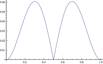
Figure 1. Plot of $D({\bf p})$ for ${\bf p}=(x,1-x)$, as a function of $x\in[0,1]$.

5.2. Dimension $n=2$: three colors of socks

The case $n=2$ can be set up similarly to $n=1$, but now we have three cases of possible signs underlying absolute values. Each case is a smooth, two-dimensional surface, and we find extremes by checking all critical values arising from points where the gradient vanishes, and on the boundary. To avoid subscripts, we switch notation from ${\bf p}=(p_{0},p_{1},p_{2})$ to ${\bf p}=(a,b,c)$, and define

$$f(a,b,c):=a^{2}(1+2(b+c)+6bc),$$

$$T(a,b,c)=\frac{a^{2}}{a^{2}+b^{2}+c^{2}}-f(a,b,c),$$

so that when ${\bf p}=(a,b,c)$, with $a$ being the probability that a single sock has color 0, $T(a,b,c)=\mathbb{P}(X=0)-\mathbb{P}(Y=0)$. Note that $T(a,b,c)=T(a,c,b)$. Exchanging the roles among colors 0, 1, 2, we have $T(b,a,c)=\mathbb{P}(X=1)-\mathbb{P}(Y=1)$ and $T(c,a,b)=\mathbb{P}(X=2)-\mathbb{P}(Y=2)$. From Definitions 1 and 2, when ${\bf p}=(a,b,c)$,

$$2D({\bf p})=|T(a,b,c)|+|T(b,a,c)|+|T(c,a,b)|.$$

The expression above has the form $|T_{1}|+|T_{2}|+|T_{3}|$, and the absolute value function is an obstacle to taking the gradient. But by taking the eight cases for the sign, each of the expressions $\pm T_{1}\pm T_{2}\pm T_{3}$ is a rational function.

A straightforward parameterization of the two-dimensional set of probabilities $(a,b,c)$ would have $a\geq b\geq 1-a-b\geq 0$, implying that $T_{1}\geq 0$ and $T_{3}\leq 0$, so that there are only two cases, according to the sign of $T_{2}$. A major obstacle to this approach is the boundary, which is complicated, so instead we parameterize in terms of $(x,y)\in[0,1]^{2}$ as follows:

$${\bf p}(x,y)=(a,b,c)\ \mbox{where }t=1+x+y,a=\frac{1}{t},b=\frac{x}{t},c=\frac{y}{t}.$$

Now taking $a=a(x,y)$ and so on, we have three functions defined on $[0,1]^{2}$,

$$T_{1}(x,y) := T(a,b,c),$$

$$T_{2}(x,y) := T(b,a,c),$$

$$T_{3}(x,y) := T(c,a,b).$$

The total variation distance is given by

(12) $$2d_{\rm TV}(X,Y)=|T_{1}(x,y)|+|T_{2}(x,y)|+|T_{3}(x,y)|.$$

Since $1\geq x,y$, we have $a\geq b,c$ and since the largest mass is at 1, we know that for all $x,y\in[0,1]$, $T_{1}(x,y)\geq 0$.

We can eliminate the case $T_{1}\geq 0,T_{2}\geq 0$ and $T_{3}\geq 0$, as this implies $T_{1}=T_{2}+T_{3}=0$ since $T_{1}+T_{2}+T_{3}=0$. By Lemma 2 this case gives $D({\bf p})=0$, not of interest in the search for the maximum value. There are three remaining cases of sign to consider. Let

$$d_{1}(x,y) = T_{1}(x,y)+T_{2}(x,y)-T_{3}(x,y),$$

$$d_{2}(x,y) = T_{1}(x,y)-T_{2}(x,y)+T_{3}(x,y),$$

$$d_{3}(x,y) = T_{1}(x,y)-T_{2}(x,y)-T_{3}(x,y).$$

Then $\max d_{\rm TV}(X,Y)=\max(d_{1},d_{2},d_{3})$, and so it suffices to check the maximum values of each of these rational functions.

Let us consider $g(x,y):=d_{1}(x,y)$. Since $g$ is a rational function in two variables, it is elementary to calculate the partial derivatives with respect to $x$ and $y$, denoted $g_{x}$ and $g_{y}$, respectively. What is not so elementary is finding all solutions $(x,y)$ to the system $g_{x}(x,y)=g_{y}(x,y)=0$. This set, $V(g_{x},g_{y}):=\{(x,y):g_{x}=g_{y}=0\}$, also known as the affine variety defined by $g_{x},g_{y}$, is what we wish to find; a good introductory text on this subject is [3].

Continuing with this example, even though $g_{x}$ and $g_{y}$ are rational functions, when each is rationalized it is clear that for $x,y\geq 0$ the denominator is always positive, and hence plays no role in characterizing the set of points in the variety $V(g_{x},g_{y})\cap[0,1]^{2}$. Thus we may simply find the variety of the numerators restricted to $[0,1]^{2}$, denoted $h_{x}$ and $h_{y}$, respectively, which are bivariate polynomials.

A generalization to the Theorem of Algebra due to Bezout (see for example Chapter 5, Section 7 of [3]) can be used to verify that all solutions have been found. In this case, after dividing out by a common factor of $x$, the two polynomials each have total degree 7. Bezout’s theorem guarantees $7\times 7=49$ solutions total including multiplicities, but some of these are solutions “at infinity.” Mathematica^® finds a set of 19 unique, easily-verified solutions; when including multiplicities, this accounts for 39 of the total solutions. By hand we can find 10 solutions at infinity, so all 49 solutions have been addressed.

We obtain the largest value of $d_{\rm TV}$ from the point $(x,y)$ given by

$$x\in(0,1): \ \ 1+4x-14x^{2}-4x^{3}-34x^{4}+20x^{5}=0,$$

$$y: \ \ y=x,$$

(13) $$\begin{split}2d_{\rm TV}=z\in(0,0.2):&\ \ \ \ 32000+168192z\\ &-4557600z^{2}+14567472z^{3}\\ &-821583z^{4}+314928z^{5}=0.\end{split}$$

This solution is of the form

$${\bf p}=\left(x_{2},\frac{1-x_{2}}{2},\frac{1-x_{2}}{2}\right)$$

for the value of $x_{2}\in[0.5,0.6]$ that solves $-5+42x_{2}-114x_{2}^{2}+168x_{2}^{3}-153x_{2}^{4}+54x_{2}^{5}=0$, with

(14) $$x_{2}\doteq 0.582011,\ \ \ D({\bf p})\doteq 0.0842942;$$

the exact value of $D({\bf p})$ given by Equation (13).

6. Conjectures about the largest possible discrepancy

The weakest conjecture is that there is some nontrivial upper bound on discrepancy. Formally, we define the universal constant for the pair discrepancy by

(15) $$\ell_{0}:=\sup_{\bf p}D({\bf p}),$$

where the supremum is over all distributions ${\bf p}$ on a finite or countable set of colors. Since total variation distance is always less than or equal to 1, trivially $\ell_{0}\leq 1$, and the conjecture is

Conjecture 1.

The constant defined by (15) is strictly less than 1, i.e.,

(16) $$\ell_{0}<1.$$

6.1. Conjectures for a finite number of colors

If there are a finite number of colors, say $n+1$ with $n\geq 0$, then we can relabel the colors as $0,1,\ldots,n$ so that ${\bf p}=(p_{0},\ldots,p_{n})$ with

(17) $$p_{0}\geq p_{1}\geq\cdots\geq p_{n}\geq 0,\ p_{0}+p_{1}+\cdots+p_{n}=1.$$

Given $n>0$, and $x\in[\frac{1}{n+1},1)$, let

(18) $${{\bf p}(n,x)}=\left(x,\frac{1-x}{n},\ldots,\frac{1-x}{n}\right),$$

which, due to $x\in[\frac{1}{n+1},1)$, satisfies (17).

With the notation (18), the result of Section 5.2 may be summarized as: for $n=2$, over all probability distributions on $n+1$ colors standardized to satisfy (17), the maximum value of $D({\bf p})$ is achieved, uniquely, at ${\bf p}={\bf p}(2,x)$, with $x=x_{2}$ as specified by (14).

For each $n>0$, (18) defines a one parameter family of probability distributions. At the endpoint $x=1/(n+1)$, ${{\bf p}(n,x)}$ is a uniform distribution. Now suppose that $x\in(1/(n+1),1)$, so that ${{\bf p}(n,x)}$ has $p_{0}>p_{1}=p_{2}=\cdots=p_{n}>0$. It is obvious from (2) that $\mathbb{P}(X=0)>\mathbb{P}(X=1)=\cdots=\mathbb{P}(X=n)>0$, and Lemma 1 implies that $\mathbb{P}(Y=0)>$ $\mathbb{P}(Y=1)=\cdots=\mathbb{P}(Y=n)>0$. That is, both $X$ and $Y$ have distributions in the same one parameter family. Finally, (7) implies that $\mathbb{P}(X=0)>\mathbb{P}(Y=0)$, while for $i=1$ to $n$, $\mathbb{P}(X=i)<\mathbb{P}(Y=i)$, and hence using (2), for each $n>0$ and $x\in(\frac{1}{n+1},1)$, ${\bf p}={\bf p}(n,x)$ has the simplified expression for its discrepancy,

$$D({\bf p}) =\mathbb{P}(X=0)-\mathbb{P}(Y=0)$$

(19) $$=\frac{x^{2}}{x^{2}+\frac{(1-x)^{2}}{n}}-x^{2}\sum_{k=0}^{n}(k+1)!\binom{n}{k}\left(\frac{1-x}{n}\right)^{k}.$$

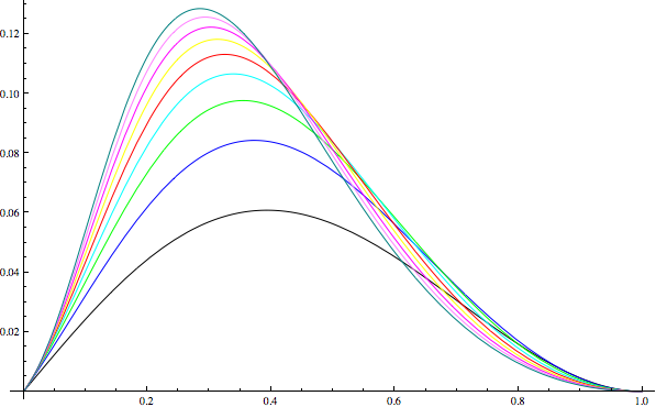
Figure 2. $D({\bf p})$ for the one parameter families (18), $n=1$ to 9. For each $n$, we plot $\frac{n+1}{n}x-\frac{1}{n}$ versus $D({\bf p}(x,n))$, so that all 9 graphs have domain [0,1].

Conjecture 2.

For every nonnegative integer $n$, among all probability distributions on $n+1$ colors, the maximum value of $D({\bf p})$ is achieved by a distribution of the form ${{\bf p}(n,x_{n})}$.

A slightly stronger conjecture is the following:

Conjecture 3.

For every nonnegative integer $n$, among all probability distributions on $n+1$ colors, the maximum value of $D({\bf p})$ is achieved uniquely by ${{\bf p}(n,x_{n})}$, where $x_{n}={\rm argmax}_{x}\ D({{\bf p}(n,x)})$.

We cannot prove Conjecture 2, but we believe it to be true, for the following reasons.

1. It is true, trivially for $n=0$ and $n=1$, and by Section 5.2, for $n=2$.

2. By broad analogy, many symmetric payoff functions achieve their extreme values at points with lots of symmetry. Indeed, Theorem 1 asserts that for each $n$, $D({\bf p})$ achieves its minimum value, zero, at the uniform distribution, corresponding to the maximum conceivable symmetry in ${\bf p}$, while the family in (18) corresponds to breaking symmetry somewhat, but as little as possible.

3. The one parameter family (18) shows up in other extremal problems which share the feature that the labels on the colors are irrelevant, and only the values of the probabilities matter. In particular, in information theory, the one parameter families show that “Fano’s inequality is sharp;” see Cover and Thomas [2], (2.135) on page 40.

4. For the moderate values $n=3,4,\ldots,8$, when generating a million random points from the $n$-dimensional region specified by (17), the largest observed $D({\bf p})$ in the sample came from a ${\bf p}$ that was close, by eye, to the form of (18).

The table below summarizes approximate extreme values under the one parameter families (18) for $n=1,\ldots,9$, using the notation $x_{n}={\rm argmax}_{x}D({\bf p}(n,x))$.

$$\begin{array}[]{ll}x_{1}=0.6966599465951643196&D(x_{1})=0.06084679923181354776\\ x_{2}=0.5820110139097399105&D(x_{2})=0.08429419234614604446\\ x_{3}=0.5160030571683498864&D(x_{3})=0.09766297359542326758\\ x_{4}=0.4710812367633940106&D(x_{4})=0.10661363736945495196\\ x_{5}=0.4376598564845561514&D(x_{5})=0.11316011048732238932\\ x_{6}=0.4113811479448445739&D(x_{6})=0.11822473613430355437\\ x_{7}=0.3899258770101118464&D(x_{7})=0.12229838762442936532\\ x_{8}=0.3719239304877958135&D(x_{8})=0.12566994796517442344\\ x_{9}=0.3565033913388721410&D(x_{9})=0.12852218802677888163\\ \end{array}$$

Figure 2 shows, for $n=1$ to 9, $D({\bf p}(x,n))$ for $x\in[\frac{1}{n+1},1]$; the graph plots $\frac{n+1}{n}x-\frac{1}{n}$ versus $D({\bf p}(x,n))$, so that all 9 graphs use the same domain, [0,1].

7. Limit analysis of the one parameter family

Theorem 2.

For $c\in(0,\infty)$ define

(20) $$\ell(c)=\frac{c^{2}}{1+c^{2}}-\int_{0}^{\infty}c^{2}te^{-ct-t^{2}/2}\,dt.$$

For any $c\in(0,\infty)$ and $n>1/c^{2}$, let ${\bf p}^{(n)}={\bf p}(n,c/\sqrt{n})$ be the distribution governed by (18) with $x=c/\sqrt{n}$. Then

(21) $$\lim_{n\to\infty}D({\bf p}^{(n)})=\ell(c),$$

where $\ell$ is defined by (20).

Proof.

Extend Method 2 beyond the time of the first matching pair; i.e., pick socks forever. For each color $i$ let $N_{i}$ be the number of sock picks needed to get the second sock of color $i$. As the color varies, these random variables are dependent, since for any two distinct colors $i,j$ and time $n\geq 2$, $0=\mathbb{P}(N_{i}=N_{j}=n)<\mathbb{P}(N_{i}=n)\,\mathbb{P}(N_{j}=n)$. There is a standard technique to deal with this dependence, used in Markov chains, which is to take a sequence of independent exponentially distributed holding times $Y_{1},Y_{2},\ldots$, with $\mathbb{P}(Y_{n}>t)=e^{-t}$, and declare that the $n$th sock arrives at time $Y_{1}+Y_{2}+\cdots+Y_{n}$. With values in $(0,\infty)$, the time $T_{i}$ at which color $i$ is first seen for the second time can be expressed as $T_{i}=Y_{1}+\cdots+Y_{N_{i}}$. The distribution of the color of the first matching pair found, initially specified by (3), can also be expressed as

$$\mathbb{P}(Y=i)=P(T_{i}<\min_{j\neq i}T_{j}).$$

For each color $i$, the times at which socks of color $i$ arrive form a Poisson arrivals process with rate $p_{i}$, and as the color varies, these processes are mutually independent; in particular the second arrival times $T_{i}$ are mutually independent.

We are considering socks distributed according to ${\bf p}(n,c/\sqrt{n})$, that is, with $y:=(1-c/\sqrt{n})$,

(22) $$p_{0}=c/\sqrt{n},p_{1}=y/n,p_{2}=y/n,\ldots,p_{n}=y/n.$$

Speed up time by a factor of $\sqrt{n}$; now socks of color 0 arrive at rate $c$, and for each other color $i=1$ to $n$, socks of color $i$ arrive at rate $p_{i}\sqrt{n}=y/\sqrt{n}$. For $t>0$, and for each $i=1$ to $n$, the number $Z$ of socks of color $i$ collected by time $t$ is Poisson with parameter $\lambda=ty/\sqrt{n}$, and the event $\{T_{i}>t\}$ is the event $\{Z<2\}=\{Z=0$ or 1}, with probability

$$\mathbb{P}(T_{i}>t) = \mathbb{P}(Z=0)+\mathbb{P}(Z=1)$$

$$= e^{-\lambda}(1+\lambda)$$

$$= \exp\left(-\frac{ty}{\sqrt{n}}\right)\left(1+\frac{ty}{\sqrt{n}}\right)$$

$$= 1-\frac{t^{2}y^{2}}{2n}+O(n^{-3/2}).$$

The easy way to see the result above is to argue that $\lambda$ is small, so $e^{-\lambda}(1+\lambda)=(1-\lambda+\lambda^{2}/2-\lambda^{3}/6+\cdots)(1+\lambda)=1-\lambda^{2}+\lambda^{2}/2+O(\lambda^{3})=1-\lambda^{2}/2+O(\lambda^{3})$.

The event $\{\min(T_{1},\ldots,T_{n})>t\}$ is the intersection of the events $\{T_{i}>t\}$, so using the mutual independence, together with $y\to 1$, for each $t>0$,

$$\mathbb{P}(\min(T_{1},\ldots,T_{n})>t) = \mathbb{P}(T_{1}>t)^{n}=\left(1-\frac{t^{2}y^{2}}{2n}+O(n^{-3/2})\right)^{n}$$

$$\to \exp(-t^{2}/2).$$

Finally, we argue that the density of $T_{0}$, the second arrival time in a Poisson process with rate $c$, is given by

$$f(t)=c^{2}te^{-ct}.$$

This is a standard fact, known to some as the density of the Gamma distribution with shape parameter 2 and scale parameter $c$. Using the independence of $T_{0}$ and $\min(T_{1},\ldots,T_{n})$, we can condition on the value $t$ for $T_{0}$ to get

(24) $$\mathbb{P}_{n}(Y=0) = \mathbb{P}(\min(T_{1},\ldots,T_{n})>T_{0})$$

$$= \int_{0}^{\infty}\mathbb{P}(\min(T_{1},\ldots,T_{n})>t)f(t)\ dt$$

$$= \int_{0}^{\infty}\mathbb{P}(\min(T_{1},\ldots,T_{n})>t)\ c^{2}te^{-ct}\ dt$$

$$\to \int_{0}^{\infty}c^{2}te^{-ct}e^{-t^{2}/2}dt.$$

The above amounts to a calculation of the limit, as $n\to\infty$, of $\mathbb{P}_{n}(Y=0)$, corresponding to Method 2 when the underlying colors come from (22).

Of course, we must justify the passage to the limit in (24). Here we have $f_{n}(t):=\mathbb{P}(\min(T_{1},\ldots,T_{n}))\to\exp(-t^{2}/2)=:f(t)$ point-wise, for each $t>0$, but we claim in (24) that the integrals also converge. If we interpret the (improper) integral as the Lebesgue integral, then we can invoke the Monotone Limit Theorem: it is easy to check that $f_{n}(t)\geq f_{n+1}(t)\geq 0$ for all $n$, and that $\int f_{1}(t)dt<\infty$, hence $\int f_{n}(t)\,dt\to\int f(t)\,dt$.

Interpreting the improper integral as a Riemann integral requires more work to justify passage to the limit in (24), and is left as an exercise; see for example Chapter 7, Exercise 12 of Rudin [8].

For Method 1 the calculation is easier: using (1) we have $f_{2}=p_{0}^{2}+p_{1}^{2}+\cdots+p_{n}^{2}=(c/\sqrt{n})^{2}+n(y/n)^{2}=c^{2}/n+y^{2}/n$ and

$$\mathbb{P}_{n}(X=0)=\frac{p_{0}^{2}}{f_{2}}=\frac{c^{2}/n}{c^{2}/n+y^{2}/n}=\frac{c^{2}}{c^{2}+y^{2}}\to\frac{c^{2}}{c^{2}+1}.$$

At (19) we had already argued that once $n$ is large enough that $p_{0}>p_{1}$ we have the simplification, for our one parameter family, that $D({\bf p}^{(n)})=\mathbb{P}_{n}(X=0)-\mathbb{P}_{n}(Y=0)$. Combining this calculation of $D({\bf p}^{(n)})$ with the limit values derived for $\mathbb{P}_{n}(Y=0)$ and $\mathbb{P}_{n}(X=0)$, (21) follows. ∎

We note that instead of invoking Poissonization, as in the above proof, one can argue directly with the explicit expression in (19), to show that under $x=c/\sqrt{n}$ and $k=t\sqrt{n}$, the sum in (19) is a Riemann approximation for $\int_{0}^{\infty}c^{2}te^{-ct}e^{-t^{2}/2}dt$.

8. Discussion

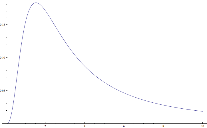
Figure 3. Plot of $c$ versus $\ell(c)$ for $c=0$ to 10. The maximum occurs at $c_{0}\doteq 1.514$ and has value $\ell(c_{0})\doteq 0.18320.$

If Conjecture 2 is true, it will follow that Conjecture 1 is also true, with the value of the universal constant for a pair of socks given by

(25) $$\ell_{0}=\sup_{c}\ell(c)=0.1832000624087106\ldots\ .$$

The argument requires two parts. The first part is to show that $\ell_{0}$, defined in (15) as the sup of $D({\bf p})$ over all discrete distributions, is equal to the sup over distributions with finite support. This is “soft” analysis, showing first that ${\bf p}\mapsto D({\bf p})$ is continuous, hence given ${\bf p}$ with discrepancy greater than $\ell_{0}-\varepsilon$ we can find a nearby distribution ${\bf p}^{\prime}$ with finite support, close enough to ${\bf p}$ to guarantee that its discrepancy is greater than $\ell_{0}-2\varepsilon$. The second part, giving the concrete value for $\ell_{0}$, uses compactness: given distributions ${\bf p}^{(n)}={{\bf p}(n,x_{n})}$ with discrepancies converging to $\ell_{0}$, the values $c_{n}:=x_{n}\sqrt{n}\in[0,\infty]$, $n\geq 1$, lie in a compact set, and hence there must be convergent subsequences. If $c_{n_{k}}\to c_{0}$ and $c_{0}\in(0,\infty)$, then the proof of Theorem 2 already shows that the associated discrepancies converge to $\ell(c_{0})$. If $c_{n_{k}}\to c_{0}$ with $c_{0}=0$ or $c_{0}=\infty$, a small extension of the proof of Theorem 2 would show that the associated discrepancies would converge to 0. So indeed, $c_{n}\to c_{0}$ and $D({\bf p}^{(n)})\to\ell(c_{0})$.

9. Shoes instead of socks: a matching left-right pair

Suppose, instead of wanting to collect a pair of matching socks, we want a pair of matching shoes. Naturally, this means one left shoe, and one right shoe, both of the same color. There are two reasonable ways to extend our study to this situation.

9.1. One distribution for left colors, another distribution for right colors

The setup here involves two discrete probability distributions, say ${\bf p}$ for the color $S$ of a left shoe, and ${\bf q}$ for the color $S^{\prime}$ of a right shoe. The analog of (1) is

(26) $$f_{2}=\mathbb{P}(S=S^{\prime})=\sum_{i}\mathbb{P}(S=S^{\prime}=i)=\sum_{i}p_{i}\,q_{i}$$

for the probability that a random left shoe and a random right shoe match. We require that for at least one value $i$, $p_{i}q_{i}>0$. The analog of (2) is the Method 1 distribution for the color $X=X({\bf p},{\bf q})$ of a matching left-right pair

(27) $$\mathbb{P}(X=i)=\mathbb{P}(S=i|S=S^{\prime})=\frac{p_{i}q_{i}}{f_{2}}.$$

For method 2, we assume that at times $1,3,5,\ldots$, one left shoe is collected, and at times $2,4,6,\ldots$, one right shoe is collected. Suppose that at time $k-1$, there is not yet a matching left-right pair, but at time $k$, there is; then $Y=Y({\bf p},{\bf q})$ is the color of the shoe collected at time $k$.

The analog of discrepancy is now

(28) $$D({\bf p},{\bf q})=d_{\rm TV}(X({\bf p},{\bf q}),Y({\bf p},{\bf q})).$$

It is fairly easy to see that for this situation, the analog of Conjecture 1 is false; that is, the supremum of the discrepancy over all pairs of distributions is no smaller than the trivial upper bound on total variation distance:

(29) $$1=\sup_{{\bf p},{\bf q}}D({\bf p},{\bf q}).$$

We give a brief sketch of a proof of (29): with $a=a(n)=n^{-1/4}$ and $b=b(n)=n^{-2/3}$ let ${\bf p}={\bf p}(n,a)$ and ${\bf q}={\bf p}(n,b)$; in other words, $p_{0}=\mathbb{P}(S=0)=a$, $q_{0}=\mathbb{P}(S^{\prime}=0)=b$ and for $i=1$ to $n$, $p_{i}=\mathbb{P}(S=i)=(1-a)/n$, $q_{i}=\mathbb{P}(S^{\prime}=i)=(1-b)/n$, with $a=n^{-1/4}$, $b=n^{-2/3}$. We have $p_{0}q_{0}=n^{-11/12}$ and

$$\sum_{i=1}^{n}p_{i}q_{i}=n\frac{1-a}{n}\,\frac{1-b}{n}\sim\frac{1}{n}=o(p_{0}q_{0}),$$

so the Method 1 distribution converges to point mass at color 0, i.e., $\mathbb{P}_{n}(X=0)\to 1$. To see that the Method 2 distribution has, in the limit, probability zero of getting color 0, consider collecting alternately left and right shoes forever. At time $m=2n^{5/8}$, we will have collected $n^{5/8}$ left and $n^{5/8}$ right shoes. Thanks to the small value $q_{0}=b=n^{-2/3}$, we expect only $n^{-1/24}$ left shoes of color 0 at time $m$, so with high probability, we do not yet have a matching pair of color 0. But, at time $m$, for each color $i=1$ to $n$, the number of left shoes of color $i$ is Binomial($m,(1-a)/n$), and hence is greater than zero with probability asymptotic to $m/n\sim n^{-3/8}$. Independently, the number of right shoes of color $i$ is greater than zero with probability asymptotic to $n^{-3/8}$; hence the probability of at least one pair of color $i$ is asymptotic to $n^{-3/4}$. The number $W$ of colors $i>0$ for which we have a pair has $\mathbb{E\,}W\sim n^{1/4}$, and the $n$ events are negatively correlated with each other, so ${\rm Var\,}W<\mathbb{E\,}W$. By Chebyshev’s inequality, $\mathbb{P}(W=0)\leq{\rm Var\,}W/(\mathbb{E\,}W)^{2}=O(n^{-1/4})$. So at time $m$, we are unlikely to have any pair of color 0, and unlikely not to have at least one pair of some other color, hence $\mathbb{P}_{n}(Y=0)\to 0$.

9.2. With the constraint ${\bf p}={\bf q}$

Now suppose that we declare that the distribution ${\bf p}$ for left shoes and the distribution ${\bf q}$ for right shoes must be equal. This does not reduce consideration of the distribution of a matching pair to the situation for socks; under the alternating left-right procedure, if we get a blue left shoe at time 1, a red right shoe at time 2, and another blue left shoe at time 3, then we still have not collected a matching pair.

The analog of Conjecture 1, for the situation of a matching left-right pair of shoes under the constraint of equal distributions, is plausible:

Conjecture 4.

(30) $$\sup_{\bf p}D({\bf p},{\bf p})<1.$$

Furthermore, we can even propose a value for the universal constant for shoes, given by the left side of (30). It comes from an analog of Theorem 2. This analog of Theorem 2 is easiest to understand without the constraint ${\bf p}={\bf q}$.

Theorem 3.

For $a,b\in(0,\infty)$ define

(31) $$\ell(a,b)=\frac{ab}{1+ab}-\int_{0}^{\infty}\left(ae^{-at}+be^{-bt}-(a+b)e^{-(a+b)t}\right)e^{-t^{2}}\,dt.$$

For $a,b>0$ and sufficiently large $n$, let

(32) $${\bf p}^{(n)}={\bf p}(n,a/\sqrt{n}),\ {\bf q}^{(n)}={\bf q}(n,b/\sqrt{n})$$

as in (18). Then

(33) $$\lim_{n\to\infty}D({\bf p}^{(n)},{\bf q}^{(n)})=\ell(a,b).$$

Proof.

The argument closely follows the proof for Theorem 2. We omit details, apart from sketching the main differences: under the distributions in (32), collecting left-right pairs with mean $1/\sqrt{n}$ holding times between pairs, the left shoes of color 0 form a rate $a$ Poisson process, the right shoes of color 0 form a rate $b$ Poisson process; $\mathbb{P}($no left 0 by time $t)=e^{-at}$, $\mathbb{P}($no right 0 by time $t)=e^{-bt}$, and in the limit, the two processes are independent, so $\mathbb{P}($no left 0 and no right 0 by time $t)=e^{-(a+b)t}$. Inclusion-exclusion and differentiation leads to the limit density of the time $T_{0}$ at which a left-right pair of color 0 is found, $f(t)=\left(ae^{-at}+be^{-bt}-(a+b)e^{-(a+b)t}\right)$, instead of the $c^{2}te^{-ct}$ of Theorem 2. At time $t$, for each of the $n$ other colors we expect, asymptotically, $t/\sqrt{n}$ instances on the left, and $t/\sqrt{n}$ on the right, with $t^{2}/n$ for the asymptotic chance of having a pair. This leads to $\mathbb{P}(\min(T_{1},\ldots,T_{n})>t)\to\exp(-t^{2})$, instead of the $\exp(-t^{2}/2)$ of Theorem 2. ∎

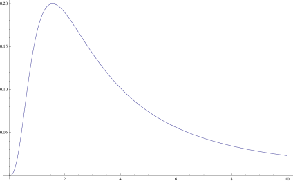
Figure 4. Plot of $\ell(a,a)$, the limit discrepancy $D({\bf p},{\bf q})$ when ${\bf p}={\bf q}={\bf p}(n,a/\sqrt{n})$. The maximum value $0.19980867\ldots$ occurs at $a=1.562239\ldots$.

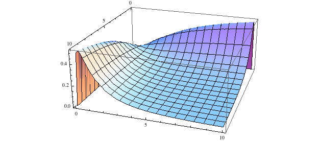
Figure 5. Plot of $\ell(a,b)$, the limit discrepancy $D({\bf p},{\bf q})$ when ${\bf p}={\bf p}(n,a/\sqrt{n})$ and ${\bf q}={\bf p}(n,b/\sqrt{n})$. The curve in Figure 4 lies along the diagonal, splitting the plot into two symmetric pieces.

While we do not have evidence for the analog of Conjecture 2 — indeed, it seems daunting to deal with the analog of Section 5.2, for left-right pairs under equal distribution for left and right — the analog of Conjecture 1 combined with (25) is the following plausible conjecture. See Figure 4 for the source of the constant $.1998\ldots$ .

Conjecture 5.

$$\sup_{\bf p}D({\bf p},{\bf p})=\max_{a}\ell(a,a)\doteq 0.199808674053.$$

References

- [1] Richard Arratia and Stephen DeSalvo. Probabilistic divide-and-conquer: a new exact simulation method, with integer partitions as an example. arXiv:1110.3856v2 [math.PR], 2011.
- [2] Thomas M. Cover and Joy Thomas. Elements of Information Theory. Wiley, 1991.
- [3] David A. Cox, John Little, and Donal O’Shea. Ideals, Varieties, and Algorithms: An Introduction to Computational Algebraic Geometry and Commutative Algebra, 3/e (Undergraduate Texts in Mathematics). Springer-Verlag New York, Inc., Secaucus, NJ, USA, 2007.
- [4] William Feller. An Introduction to Probability Theory and Its Applications, volume 1. Wiley, January 1968.
- [5] G.B. Folland. Real analysis: modern techniques and their applications. Pure and applied mathematics. Wiley, 1999.
- [6] G.F. Lawler. Introduction to Stochastic Processes. Chapman & Hall Probability Series. Chapman & Hall, 1995.
- [7] Mathematica. Mathematica Edition: Version 8.0. Wolfram Research, Inc., Champaign, IL, 2010.
- [8] R. Walter. Principles of Mathematical Analysis. International Series in Pure and Applied Mathematics Series. McGraw-Hill International, 1976.