BoA: a versatile software for bolometer data reduction

Abstract

Together with the development of the Large APEX Bolometer Camera (LABOCA) for the Atacama Pathfinder Experiment (APEX), a new data reduction package has been written. This software naturally interfaces with the telescope control system, and provides all functionalities for the reduction, analysis and visualization of bolometer data. It is used at APEX for real time processing of observations performed with LABOCA and other bolometer arrays, providing feedback to the observer. Written in an easy-to-script language, BoA is also used offline to reduce APEX continuum data. In this paper, the general structure of this software is presented, and its online and offline capabilities are described.

1 INTRODUCTION

The Atacama Pathfinder Experiment (APEX) is a novel 12 m single dish sub-millimeter (submm) telescope, operating from the Chanjnantor Plateau in Chile since 2006[1]. It is equipped with heterodyne receivers covering frequencies of 230 GHz to 1.4 THz (wavelengths 200 microns to 1.3 mm), and several large arrays of bolometers: the APEX-SZ camera[2] at a wavelength of 2 mm, LABOCA (870 $\mu$m) and SABOCA (350 $\mu$m). More bolometer arrays are expected to come in the near future.

The Large APEX Bolometer Camera[3] (LABOCA) consists of 295 bolometer detectors operating at 870 $\mu$m. They are arranged in a hexagonal pattern, with two-beam spacing between individual detectors, resulting in a field of view of 11.4^′ in diameter. As part of the development of LABOCA by the Bolometer Group in the Max-Planck-Institut für Radioastronomie (MPIfR), a new data reduction software has been written for processing bolometer data acquired at APEX: the Bolometer array data Analysis software (BoA).

One reason for the need of a new software package was the new data file format. The raw data are written by the APEX Control System (APECS[4]) in MB-FITS (Multi-Beam FITS) format. This format has been designed and constantly extended during the first few years of APEX operations. In addition, one of the main drivers for the development of BoA has been to provide high modularity, and an environment where the user can run existing scripts, but also develop his/her own scripts to extend the capabilities of the software. As such, BoA has been written in a scripting language, with the aim that each processing function can easily be modified for specific needs.

BoA is an open source software. It is distributed under the terms of the GNU General Public License. The source code and the external libraries required to run BoA can be downloaded from a dedicated page at the MPIfR website. The software comes with a user and reference manual, as well as a set of typical reduction scripts for LABOCA and SABOCA. In the present paper, I will describe the general structure of BoA, and highlight its main functionalities. A typical pipeline for reducing LABOCA data is discussed in Section 5.

2 Structure of the software

2.1 Programming language

The BoA software is written in object oriented languages: most of the code is in Python, including many external packages, while the most computing demanding tasks are written in FORTRAN95.

The BoA source code is made of several modules, that define functionalities for: raw data reading, analysis tools, plotting procedures, and data processing. The latter applies to a so-called data object (see below), which is created when BoA is started. More than one data object can reside at a given time in BoA (with different variable names). They can be dumped to binary files, in a format specific to python, and restored later, e.g. during the next BoA session.

2.2 The main data object

The main data object in BoA contains everything that may be required to process one or more data file(s). The raw data are written by the APECS[4] in MB-FITS (Multi-Beam FITS) format. Once such a data-file is read in BoA, the data object is filled up with all relevant information, which can be divided in three groups: the telescope (coordinates) data, the description of the bolometer array, and the data values themselves.

2.2.1 Telescope data

All the information related with coordinates and time is stored into the ScanParam attribute of the data object. This includes: coordinates where the telescope has been pointing, in horizontal, equatorial and galactic systems; time stamps in MJD and LST; target name and reference coordinates; sub-scans related information: sub-scans numbers, and integrations numbers they correspond to; when relevant, wobbler phases. Note that the telescope positions expressed as offsets (with respect to the reference position) in horizontal system, as they are stored in the raw data file, include the wobbler displacement, when relevant.

In addition, an array of flags is attached to the ScanParam attribute, in order to flag the data recorded by all bolometers at given times during the scan. Functions exist to flag the data in a given interval of time, or according to the position of the telescope (e.g. when the offset in Azimuth exceeds a given value). It is also possible to temporarily flag (or mask) some part of the data, and unflag it later.

2.2.2 Bolometer array

The most important information about the instrument in use is stored in the MB-FITS files: telescope name and diameter; effective observing frequency; global gain settings or attenuation factors; for an array of detectors, relative positions of the pixels, and their relative gains; reference channel number.These data are read in by BoA and stored in the BolometerArray attribute. At the time of reading, BoA also derives the nominal instrumental beam size from the telescope diameter and effective frequency.

The relative offsets between pixels and their relative gains can latter be updated in BoA, by reading a so-called RCP (Receiver Channel Parameter) file (see also Sect. 5.1.1). The values written in the MB-FITS file are the ones known to APECS at the time of observing. These may be not up-to-date, but beam maps are observed and processed regularly, in order to update the pixels positions and gains a posteriori.

Here also, an array of flags is associated with the BolometerArray attribute, to allow the user to flag all data recorded by a given pixel (or by a list of pixels).

2.2.3 Data values and weights

Finally, the data values are stored in a 2-dimensional array: the Data attribute, with size equal to number of pixels $\times$ number of integrations. At the time of reading, the values present in the file are corrected for global gain/attenuation factors. They can later be converted from instrumental units (counts) to physical units (Jy/beam), using the conversion factor that has been measured. They can also be corrected for the atmospheric attenuation, computed as exp($\tau_{z}$ / sin(El)), where $\tau_{z}$ is the zenith opacity and El is the median of the elevation during the observation.

During the reduction of an observation, the content of the Data array is permanently updated by any processing task. For example, applying a flat field divides all the data values for a given pixel by the associated relative gain. A description of the main processing tasks is given in Sect. 5.

A second array, with the same size as the Data array, contains the weights associated to the data. The user needs to explicitly tell BoA to compute these weights before building a map (Sect. 5.4). Two methods exist to compute the weights: either using natural weighting (where each pixel has a constant weight along the time, equal to 1/r.m.s.²), or using sliding weights, also equal to 1/r.m.s.², but this time computing the r.m.s. within a sliding window containing a given number of integrations. In the latter case, if all data points are flagged within a window (which can happen e.g. when masking a source), the corresponding weights are computed by interpolating between available values before and after that window.

Another 2-dimensional array contains flags, associated to individual data values. Again, it is possible to temporarily mask part of the data and unflag them later.

Finally, one attribute is attached to the main data object in order to compute and store a map (Sect. 5.4). This contains the map itself (a 2-dimensional array of pixel values), as well as a description of the map coordinates: projection system, pixel scale and limits of the map.

2.3 Associated methods

Functions have been defined to perform all kind of data processing; examples are described with more details in Sect. 5. Shortcuts have been defined, which apply to the default data object, to ease the use of these functions from the interactive prompt in python. The functionalities present in BoA include: signal plotting (Sect. 3); flat fielding and calibration (Sect. 5.1); data flagging and unflagging (Sect. 5.2); baseline and correlated noise subtraction (Sect. 5.3); filtering in the Fourier domain; computing, displaying and exporting a map (Sect. 5.4).

3 Data visualization

One of the strengths of BoA is to allow the user to visualize the data in many different ways This includes: plotting the bolometer signal vs. time (see an example in Fig. 1), displaying correlation plots (signal in each bolometer vs. signal in an arbitrary reference bolometer), plotting the mean or r.m.s. values per bolometer, computing and displaying Fourier transform of the signals. Each of these functions can display the data of all bolometers, or restricted to any number of bolometers. The user can also overlay several plots on each other, as illustrated in Fig. 1.

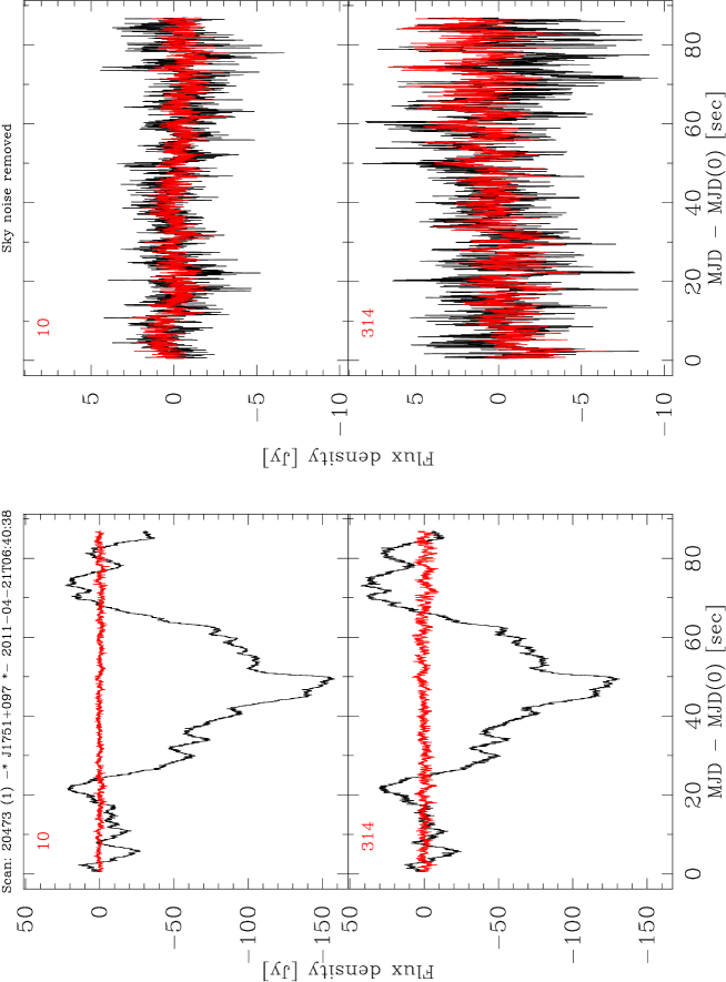
Figure 1: Example plots produced with the signal function, for two bolometers. Left: raw data (black) and data after median noise subtraction on the full array (red). Right: data after median noise subtraction on the full array (black) and then after median noise subtraction on amplifier boxes (red) - see also Fig. 3.

Once a map has been computed, the user can display the map itself, but also the coverage plane or the weight plane associated to it. BoA also provides a function to zoom into a sub-region of the map. Finally, another function allows to look at the values of individual pixels, or average values over a small region. However, BoA is not aimed at providing extensive analysis tools. Once a map has been computed (eventually co-adding several scans into one map), the user should export the result is standard FITS format, in order to use any other software to perform further analysis.

4 Online data processing

The BoA software is interfaced with the APEX Online Calibrator, which is part of APECS. The purpose of this calibrator is to automatically perform a quick reduction of almost all observations, and to provide feedback to the observer. This is of particular importance for the reduction of pointing and focus scans, since any deviation from the optimal pointing and focus settings that can be inferred from these scans should be corrected for before starting the next science observation.

4.1 Pointing scans

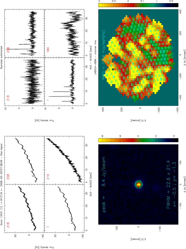
Figure 2: Example display from the online calibrator during the reduction of a pointing scan. The four panels show: signals in the reference pixel and three comparison pixels before any processing (top left). Same after correlated noise has been removed (top right). Map in horizontal coordinates built by combining all pixels (bottom left); the results of a 2D Gaussian fit are also shown: peak flux, position and size of the Gaussian profile. Finally, a map of the r.m.s. per pixel is shown (bottom right), where all used pixels are plotted at their relative positions. A quick estimate of the median value of the noise equivalent flux densities in all channels is computed and shown on top of this map.

LABOCA is operated in total-power mode, which means that, usually, no chopping secondary (wobbler) is used when observing with LABOCA. Thanks to its high sensitivity, pointing scans on bright sources ($>$10 Jy peak flux) can be performed with a single $\sim$30 s long spiral pattern. Such scans are automatically recognized as pointing scans by the online calibrator. They are processed using a quick reduction procedure: a zero-order (median) baseline is subtracted in each pixel; then pixels with excessively low r.m.s.  (dead pixels, or not seeing the sky) and the ones with very high r.m.s.  are flagged; then, the correlated noise is computed and subtracted using median estimates (see Sect. 5.3 and Fig. 3 for details); then, a map is computed, in horizontal coordinates (offsets in azimuth and elevation with respect to the nominal target position), using natural weighting. Finally, a 2-dimensional Gaussian profile is fitted on the map, in order to derive the observed position of the source.

The pointing errors ($\delta$Az, $\delta$El) derived from this fit are sent by BoA to APECS. The observer can then apply these corrections. During the reduction, the signals in the reference pixel and in three comparison pixels are plotted, as well as the map built from the processed data, together with the results of the Gaussian fitting (Fig. 2). Thus, the observer can verify that the pointing offsets computed by BoA make sense, given the quality of the map.

Correcting for the telescope pointing errors is best done as close as possible to the science target. But the sky does not contain bright pointing sources in all directions. Therefore, it is usual to do such a pointing scan on a relatively faint ($\sim$1 Jy) compact source. Then, the observer can use an existing script optimized to process observations of such moderately faint sources. The main difference compared to the online reduction of pointing scans is that more iterations of correlated noise removal are computed, in order to decrease the noise level in the final map. Then a 2-dimensional Gaussian profile is fitted on the map, and, if the source is detected with a sufficient signal-to-noise, the observer can apply the pointing corrections computed by this BoA script.

4.2 Focus scans

Focus scans have to be observed from time to time, in order to check the focus settings of the telescope, and correct for them if any deviation from the optimal position is found. This is especially important when the air temperature changes quickly, e.g. after sunrise or sunset. A focus scan consists of a number of sub-scans, where each sub-scan is a short integration (5 to 10 s) staring at a very bright source (typically the planets Venus, Saturn or Mars, the fainter planets Uranus and Neptune can also be used when the atmosphere is stable), at a given focus setting. One of the focus axis (X, Y or Z) is changed by a small amount between each sub-scan.

The online calibrator also recognizes such scans, and they are automatically processed using a quick procedure: first, a constant is subtracted from the signals in all pixels, so that they all start at zero; then, a first attempt to determine the optimal focus setting is done, by fitting a parabola to the flux observed by the reference pixel (the one that stares on the source) as a function of the focus position; then, the correlated noise is estimated and subtracted from all pixels; finally, a second parabola fit is performed to derive the optimal focus position.

Here also, the result is sent to APECS, and the observer can apply the correction computed by BoA. The signals seen by the reference pixel, plus three comparison pixels, are shown before and after sky-noise removal, as well as the results of the parabola fits. Thus, the observer can appreciate the quality of the fit, and of the sky-noise subtraction.

4.3 Science data

Most science observations conducted with LABOCA consist in maps, acquired with fast scanning patterns (either linear on-the-fly maps, or one or several spirals optimized to cover a given field; see Sect. 8 in Siringo et al.[3]). Such observations are also quickly reduced by the online calibrator, except for the very long integrations (more than $\sim$25 min.), which result in very big data files that would take too long to process, and this would slow down the full system.

For data files smaller than 100 MB (which roughly corresponds to 25 min. integration with a sampling rate of 25 Hz), the following quick reduction is performed: pixels with very low r.m.s. (dead or not seeing the sky) or with excessive noise are detected and flagged; correlated noise is computed and subtracted, with three iterations on the full array; a first-order polynomial baseline is subtracted in each pixel; spikes are detected (data-points at more than 10-$\sigma$, where $\sigma$ is the r.m.s. in a given pixel; note that very bright sources are also considered as spikes in this case), and flagged; finally, a map is computed in equatorial coordinates, using natural weighting of the individual pixels. This map is displayed, together with the r.m.s. in the map, computed in the part of the map with enough coverage to be significant (i.e. excluding the edges of the map, where the noise level quickly increases because of the sparse coverage).

5 Offline data reduction

In this section, a typical processing sequence data is presented. The structure of this pipeline is illustrated in Fig. 3. This applies to LABOCA as well as SABOCA data; example scripts are provided for both instruments with the software. They cover a range of practical cases, from faint to bright sources, and from point-like to extended; but all scripts follow the same structure, with only subtle differences in a few parameters, such as the number of iterations for sky-noise subtraction, or the masking of the source.

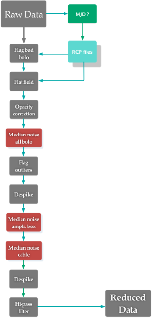
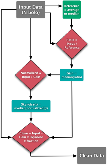
Figure 3: Left: A complete reduction sequence is shown for LABOCA data, going from the raw data to the reduced data, ready to be projected onto a map. Right: Detailed description of the median noise subtraction method. Not only the correlated noise, but also the relative gains are computed using median values.

5.1 Calibration

5.1.1 Updating receiver channel parameters

Default values for the bolometer relative gains and relative positions are contained in the raw data-file. These can be updated with more accurate values, e.g.  as derived from beam maps observed close in time to the science data. BoA provides functions to select the appropriate RCP file from a list as a function of observing time. Then, the flatfield function should be called to divide all bolometer signals by their relative gains.

5.1.2 Photometric calibration

One of the major difficulties in calibrating sub-mm data is a proper estimate of the sky opacity. This is based on, both, regular observations of skydips (where the bolometers are measuring the sky emission while the telescope is tipping from high to low elevation), and observations of primary or secondary calibrators (sources for which the flux at the observing frequency is known). Any deviation between the expected flux and the observed flux for these calibrators can thus be measured, and this calibration correction factor can be applied to the science data.

Example scripts are provided to process lists of skydips and of calibration scans, and to store the results in text files. Then, BoA provides functions to compute the sky opacity and the calibration correction factor at any given time by means of linear interpolation between the values stored in these files. This calibration should then be applied to the science data.

Sky opacities and calibration correction factors are regularly computed by the APEX staff, using default reduction scripts. These values are available online. However, users are encouraged to process the calibration scans available with their data themselves, in order to decide on their own the best calibration values. Typically, a photometric uncertainty of $\sim$10% with LABOCA and $\sim$20% with SABOCA can be achieved.

5.2 Data flagging

Several functions have been defined to flag (or to temporarily mask) part of the data, either within the 2D array of data values, or for all bolometers simultaneously in given ranges of time, or to flag some bolometers completely. For example, a function despike looks for data values that deviate by more than a number of sigma from the mean value in each bolometer time stream. Other functions provide ways to mask part of the data that correspond to a certain region of the sky, defined with a circle, or a polygon.

In addition, a function allows the user to use a map object (e.g.  the result of a previous reduction) in order to mask in the data the values that correspond to pixels in this map above a given threshold (Sect. 5.5). This is very useful when bright sources are present in the data, since their fluxes may affect some of the processing steps, such as baseline subtraction or correlated noise removal.

5.3 Correlated noise removal

Because it is working in total-power mode, at a wavelength where the emission from the atmosphere is much brighter than that from any astronomical object (except possibly the Sun), the main source of noise in LABOCA data comes from the slow variations of the atmospheric emission, also called sky-noise. Fortunately, this emission is highly correlated on the spatial scale of the detector array. BoA provides two methods to compute (and subtract) the correlated emission.

5.3.1 Median noise

The first method uses medians to compute the fraction of the signal that is correlated between pixels. Median values are a better estimator than mean values, because they are not affected by strong (compact) sources. However, extended sources, with uniform emission on spatial scales large enough so that half the pixels considered for computing the correlated “noise” see these sources, are considered as sky-noise and their flux is also subtracted from the data.

By default, this procedure proceeds in two steps (see right panel in Fig. 3: first, the relative gains between pixels are estimated, using median values of the ratios between one pixel signal and a reference signal. The reference signal can be either the signal in one particular pixel, or the average of all signals, or the median of all signals. For each pixel, the ratio between its signal and the reference signal is computed as a one-dimensional array (as a function of time or integration number), and the median value of this ratio is considered as the relative gain of this pixel, and is stored internally (but the signal is not modified according to this gain). Optionally, the user can skip this step and let the function use relative gains that were previously stored in the data object (these gains are initialized to ones by default).

As a second step, the correlated signal is estimated, also using median values: at each integration step, the median between all normalized (using the relative gains computed in the previous step) signals is considered to be the correlated noise. Finally, this correlated signal is scaled by the relative gain of each pixel, and this (or a fraction of this) is subtracted from all pixel signals.

This method can be applied to all bolometers in the array, or to sub-groups of bolometers. In the case of LABOCA, this is of particular importance to significantly reduce the noise level: the correlated noise caused by the variations of the sky emission is mostly correlated over the full field of view, but additional components of correlated noise are coming from some electronic sub-systems. In particular, groups of bolometers that are connected to a given amplifier box (corresponding to one quarter of the field of view), and sub-groups that are connected on a given flat cable (corresponding to a spatial scale of $\sim$5^′$\times$2^′, see Siringo et al.[3] for details on the electronic scheme of LABOCA) show correlated electronic noise. However, special care should be taken in order not to filter out real extended emission; when only point sources are expected, iterating several times on the correlated noise removal by groups of pixels helps in decreasing the final noise level.

5.3.2 Principal component analysis

The other correlated noise removal function is based on a principal component analysis (PCA) and filtering. Comparisons between the results obtained when applying this method, and with the median noise removal, showed that they give similar results, both with LABOCA and with APEX-SZ data. However, the effect of PCA filtering on the true astronomical signal is difficult to predict. Therefore, most results published so far based on BoA data reduction were obtained using the median noise removal method. More elaborated methods, e.g.  fitting and removing a low-order two-dimensional polynomial function across the array at each time step, can also easily be implemented in BoA.

5.4 Map making

At any time during the reduction, a map can be computed, using all or part of the data currently in memory. Three coordinate systems are implemented in BoA: Horizontal (offsets in azimuth and elevation with respect to the reference coordinate), Equatorial J2000 and Galactic coordinates. The map-making procedure computes a map by dumping and co-adding the data values on a grid of pixels, without using extra information from the redundancy within the map. By default, the map-making procedure dumps each data value into the nearest pixel; optionally, the value can be divided into the four neighbour pixels, with fractions depending on the exact location of that data point with respect to the pixel grid. The mandatory arguments for the mapping function are the limits in X and Y (when not given, default values are computed in order to encompass the full region covered by the data) and the pixel scale (default value is half the instrumental beam). The data values are co-added using a weighted average, where the weights have to be computed prior to building the maps (Sect. 2.2.3).

The resulting map can be dumped into a binary file, that can be later imported again in BoA. It can also be exported into a FITS file, with a standard FITS header containing a description of the coordinates following the WCS specification[5]. Currently, the only projection system implemented in BoA is GLS (Global Sinusoid, equivalent to the Sanson-Flamsteed - SFL - projection; see Calabretta & Greisen[6] for details). By default, the output FITS file contains three planes: the flux map, the weight map and the coverage map. The weights are computed by summing all data weights that have contributed to one given pixel. The coverage plane is similar, but considering all weights equal to one (in other words, the coverage gives the number of hits in a given pixel).

When several observations cover the same region of the sky (or if they overlap), they can be processed independently, and maps covering exactly the same region (and with the same pixel scale) can be built from each observation. These maps can then be co-added, using a weighted average, into one combined map. This “final” map can also be exported as a binary (python) file, or into a FITS file.

5.5 Iteration with source model

At the end of the reduction sequence, once a map has been computed (eventually combining several scans), it is sometimes useful to repeat the full processing in an iterative way. The result map can be used as a model to mask in the data the measurements that correspond to pixels in the map above a given threshold. It is also possible to compute a signal-to-noise map and use it as a model to mask the data points where highly significant emission has been found. The processing steps are then computed ignoring the masked data, but the results (for example subtracting a baseline) are also applied to them.

Such iterative reduction scheme is of critical importance in the presence of bright sources, for example in the Galactic plane[7]. In such complex fields, masking the data that correspond to strong emission is not the best solution, because too much data are masked when also extended emission becomes significant. Also, a drawback of masking part of the data is that spikes that sit on top of a bright source can never be identified and flagged. For these reasons, it is better to subtract a model (i.e.  the map resulting from the previous iteration) from the raw calibrated data, and then repeat the full reduction sequence.

This iterative scheme can be repeated any number of times. For example, in the case of the ATLASGAL[7] data, 15 iterations have been performed to produce the final maps. Also when no really strong source is present in the field, this iterative processing can be useful in order to recover as much extended emission as possible. This method has been used by Belloche et al.[8] on LABOCA data covering the Chamaeleon molecular cloud. They also performed extensive simulations in order to estimate the fraction of flux lost by the data processing as a function of source size and of number of iterations. The results that they present in their appendix apply to any LABOCA data processed in a similar manner, i.e.  with the median noise removal method and an iterative reduction scheme.

6 Conclusion

In the past few years, BoA has been used by an increasing number of people to process LABOCA, SABOCA and APEX-SZ data. The results have been published in major journals of astrophysics research.

Since BoA is an open-source software, anybody can contribute to its further development, either by adding functions in the source code of BoA itself, or by writing and sharing reduction scripts. Current developments at APEX and at the MPIfR include a parallelization of the most demanding processing steps, in order to make BoA able to reduce data taken with the next generation of kilo-pixels cameras.

- [1] Güsten, R., Nyman, L. Å., Schilke, P., Menten, K., Cesarsky, C., and Booth, R., “The Atacama Pathfinder EXperiment (APEX) - a new submillimeter facility for southern skies -,” A&A 454, L13–L16 (Aug. 2006).
- [2] Dobbs, M., Halverson, N. W., Ade, P. A. R., Basu, K., Beelen, A., Bertoldi, F., Cohalan, C., Cho, H. M., Güsten, R., Holzapfel, W. L., Kermish, Z., Kneissl, R., Kovács, A., Kreysa, E., Lanting, T. M., Lee, A. T., Lueker, M., Mehl, J., Menten, K. M., Muders, D., Nord, M., Plagge, T., Richards, P. L., Schilke, P., Schwan, D., Spieler, H., Weiss, A., and White, M., “APEX-SZ first light and instrument status,” New Astronomy Review 50, 960–968 (Dec. 2006).
- [3] Siringo, G., Kreysa, E., Kovács, A., Schuller, F., Weiß, A., Esch, W., Gemünd, H., Jethava, N., Lundershausen, G., Colin, A., Güsten, R., Menten, K. M., Beelen, A., Bertoldi, F., Beeman, J. W., and Haller, E. E., “The Large APEX BOlometer CAmera LABOCA,” A&A 497, 945–962 (Apr. 2009).
- [4] Muders, D., Hafok, H., Wyrowski, F., Polehampton, E., Belloche, A., König, C., Schaaf, R., Schuller, F., Hatchell, J., and van der Tak, F., “APECS - the Atacama pathfinder experiment control system,” A&A 454, L25–L28 (Aug. 2006).
- [5] Greisen, E. W. and Calabretta, M. R., “Representations of world coordinates in FITS,” A&A 395, 1061–1075 (Dec. 2002).
- [6] Calabretta, M. R. and Greisen, E. W., “Representations of celestial coordinates in FITS,” A&A 395, 1077–1122 (Dec. 2002).
- [7] Schuller, F., Menten, K. M., Contreras, Y., Wyrowski, F., Schilke, P., Bronfman, L., Henning, T., Walmsley, C. M., Beuther, H., Bontemps, S., Cesaroni, R., Deharveng, L., Garay, G., Herpin, F., Lefloch, B., Linz, H., Mardones, D., Minier, V., Molinari, S., Motte, F., Nyman, L.-Å., Reveret, V., Risacher, C., Russeil, D., Schneider, N., Testi, L., Troost, T., Vasyunina, T., Wienen, M., Zavagno, A., Kovacs, A., Kreysa, E., Siringo, G., and Weiß, A., “ATLASGAL - The APEX telescope large area survey of the galaxy at 870 m,” A&A 504, 415–427 (Sept. 2009).
- [8] Belloche, A., Schuller, F., Parise, B., André, P., Hatchell, J., Jørgensen, J. K., Bontemps, S., Weiß, A., Menten, K. M., and Muders, D., “The end of star formation in Chamaeleon I?. A LABOCA census of starless and protostellar cores,” A&A 527, A145 (Mar. 2011).