Changes of Dust Opacity with Density in the Orion A Molecular Cloud

Abstract

We have studied the opacity of dust grains at submillimeter wavelengths by estimating the optical depth from imaging at 160, 250, 350, and 500 µm from the Herschel Gould Belt Survey and comparing this to a column density obtained from the 2MASS-derived color excess $E(J-K_{\rm s})$. Our main goal was to investigate the spatial variations of the opacity due to ‘big’ grains over a variety of environmental conditions and thereby quantify how emission properties of the dust change with column (and volume) density. The central and southern areas of the Orion A molecular cloud examined here, with $N_{\rm H}$ ranging from 1.5 $\times 10^{21}$ cm^-2 to $50\times 10^{21}$ cm^-2, are well suited to this approach. We fit the multi-frequency Herschel spectral energy distributions (SEDs) of each pixel with a modified blackbody to obtain the temperature, $T$, and optical depth, $\tau_{1200}$, at a fiducial frequency of 1200 GHz (250 µm). Using a calibration of $N_{\rm H}/E(J-K_{s})$ for the interstellar medium (ISM) we obtained the opacity (dust emission cross-section per H nucleon), $\sigma_{\rm e}$(1200), for every pixel. From a value $\sim 1\times 10^{-25}$ cm² H^-1 at the lowest column densities that is typical of the high latitude diffuse ISM, $\sigma_{\rm e}$(1200) increases as $N_{\rm H}^{0.28}$ over the range studied. This is suggestive of grain evolution. Integrating the SEDs over frequency, we also calculated the specific power $P$ (emission power per H) for the big grains. In low column density regions where dust clouds are optically thin to the interstellar radiation field (ISRF), $P$ is typically $3.7\times 10^{-31}$ W H^-1, again close to that in the high latitude diffuse ISM. However, we find evidence for a decrease of $P$ in high column density regions, which would be a natural outcome of attenuation of the ISRF that heats the grains, and for localized increases for dust illuminated by nearby stars or embedded protostars.

‘

1. Introduction

Thermal dust emission is optically thin at submillimeter wavelengths. As such, it provides a useful probe of the interstellar medium (ISM) and the embedded filamentary and clumpy structures within it which relate to the early stages of star formation. These structures are being revealed in exquisite detail by the Herschel Gould Belt Survey (HGBS, André et al., 2010), the Herschel imaging survey of OB Young Stellar objects (HOBYS, Motte et al., 2010), and the Herschel infrared Galactic Plane Survey (Hi-GAL, Molinari et al., 2010). The best spatial resolution is obtained by the HGBS given the relative proximity of the target molecular clouds.

For quantitative measurements of the total column density, $N_{\rm H}$, and for assessment of the mass and gravitational (in)stability of any structures in the molecular cloud, the dust opacity is required. Evidence for significant environmental changes in opacity, ranging over an order of magnitude, has already been presented; see, e.g., Juvela et al. (2011); Planck Collaboration et al. (2011a, b); Martin et al. (2012). Using new HGBS data, our goal here is to investigate whether or not there is any systematic dependence of opacity on column (and volume) density.

Theoretically, dust grains are expected to evolve in a sufficiently dense medium, by aggregation or growth of ice mantles. Certainly this is the conclusion of a number of numerical simulations of dust evolution in dense ISM environments (e.g., Ossenkopf & Henning, 1994; Ormel et al., 2011). Given the complexity of dust in the ISM, however, a completely ab initio prediction for a particular environment is challenging, and so it is useful to seek observational constraints on the onset and magnitude of any environmental changes.

Volume density, not column density per se, ought to be the determinant of dust evolution. For this study we have selected the southern part of the Orion A molecular cloud imaged by the HGBS (Polychroni et al. 2012 in preparation). Its high column density, despite its relatively high Galactic latitude, $b$ $\sim$ $-$19°, suggests that the emission comes largely from a single cloud, in which case the high column density can be reasonably attributed to high volume density. Also, at least to a first approximation, the cloud should be bathed in a relatively uniform interstellar radiation field (ISRF). For this sort of analysis, such a field is therefore much more favorable than one in the Galactic plane where a wide range of conditions would be superimposed along the line of sight.

The larger (‘big’) dust grains, which account for most of the dust mass, are in thermal equilibrium with the ambient radiation field (Compiègne et al., 2011). The intensity of the thermal dust emission, when optically thin, is given by

$$I_{\nu}=\tau_{\nu}B_{\nu}(T)\equiv\sigma_{\rm e}(\nu)N_{\rm H}B_{\nu}(T),$$ (1)

where $\tau_{\nu}$ is the dust optical depth of the column of material, $B_{\nu}(T)$ is the Planck function for dust temperature $T$, $N_{\rm{H}}$ is the total hydrogen column density (H in any form), and $\sigma_{\rm e}(\nu)=\tau_{\nu}/N_{\rm H}$ is the opacity of the interstellar material (the emission cross-section per H nucleon).

Clearly, quantifying the optical depth and the opacity requires knowledge of $T$. Determination of $T$ is made possible by the multi-frequency coverage now available with the Herschel Space Observatory (Pilbratt et al., 2010), through fitting the spectral energy distribution (SED) of $I_{\nu}$. The other requirement is an independent measure of $N_{\rm H}$. Here we have used the near-infrared color excess $E(J-K_{\rm s})$ as a proxy (see Appendix A), derived from the Two Micron All Sky Survey (2MASS) data.

Another quantity that we examine (Section 5) is the ‘specific power,’ i.e., the total power per H emitted by dust grains in thermal equilibrium:

$$P=\int 4\pi\sigma_{\rm e}(\nu)B_{\nu}(T)d\nu.$$ (2)

Since in equilibrium $P$ is equal to the total energy absorbed per H, $P$ is affected by the intensity of the ISRF, which can be higher than average near a strong source of radiation, or lower than average because of attenuation in a region of high column density (without internal sources of illumination). Note how, for a given absorbed $P$, the resulting equilibrium temperature is inversely related to how efficiently grains can emit.

This paper is organized as follows. In Section 2, we briefly describe Herschel imaging of the Orion A molecular cloud using the PACS (Poglitsch et al., 2010) and SPIRE (Griffin et al., 2010) cameras. Maps of the SED fitting parameters $\tau$ and $T$ are derived in Section 3. We discuss the SED fitting, validate the fits through prediction of the 100 µm emission for comparison with observations by IRAS (Appendix B), and assess the uncertainty in $I_{\nu}$, and estimate the uncertainties of the derived parameters through Monte-Carlo simulation (Appendix C). In Section 4, we compare $\tau$ with $N_{\rm H}$ to find an estimate of the opacity (Equation (1)). It appears that the opacity grows systematically with $N_{\rm H}$, evidence for grain evolution. We examine the dependence of quantities related to $P$ in Section 5, specifically the anti-correlation between $T$ and $\tau$ and the spatial and $N_{\rm H}$ dependence of $P$. This analysis provides insight into the various interrelationships between $T$, $\sigma_{\rm e}$, and $P$ discussed in Section 6. We conclude with a summary in Section 7.

2. Herschel Observations

As part of the HGBS, three fields in the Orion A molecular cloud were mapped at a scanning speed of 60″ s^-1 in parallel mode, acquiring data simultaneously in five bands using the PACS (Poglitsch et al., 2010) and SPIRE (Griffin et al., 2010) arrays. Images were produced by the ROMAGAL map-maker (Traficante et al., 2011) and first results on the filamentary and core substructures in the two fields studied here, called Orion A-C1 and Orion A-S1, are presented by Polychroni et al. (2012). The images have angular resolutions of 9$\farcs$6, 13$\farcs$5, 18$\farcs$0, 24$\farcs$0, and 37$\farcs$0 at 70, 160, 250, 350, and 500  µm, respectively. In the following analysis we did not use the 70 µm image. Zero-point offsets added to these images, obtained by correlating with Planck and IRAS images (Bernard et al., 2010), were 8, 20, 10, and 4 MJy sr^-1 at 160, 250, 350, and 500 µm, respectively for the Orion A-C1 images and similarly 3, 14, 18, and 8 MJy sr^-1 for the Orion A-S1 images. Uncertainties in the zero-point offsets have the most effect on the SEDs of pixels with lower brightnesses, and the offsets were refined as discussed in Appendix C. Prior to fitting SEDs for each pixel, we convolved and then regridded the individual images to correspond to the lowest resolution (37$\farcs$0) on a common grid with 11$\farcs$5 pixels. Power spectra of these images follow a ‘cirrus-like’ power-law relation that decays with spatial frequency until at the highest frequencies it merges with a flat level corresponding to the noise in the map (Roy et al., 2010; Martin et al., 2010), assessed at 0.92, 0.58, 0.31, and 0.38 MJy sr^-1 for 160, 250, 350, and 500 µm, respectively.

3. Maps of $\tau$ and $T$

We parametrized the spectral dependence of the opacity (or $\tau$) as $\sigma_{\rm e}(\nu)/\sigma_{\rm e}(\nu_{0})=(\nu/\nu_{0})^{\beta}$, with a fiducial frequency $\nu_{0}=1200$ GHz (250 µm). Although HGBS consortium assumed an emissivity index, $\beta$, of 2.0, however, in this paper we adopted a fixed $\beta=1.8$ to facilitate comparison with earlier analyses (Planck Collaboration et al., 2011a; Martin et al., 2012). Treating $\beta$ as a fitting parameter does not change our results (Section 4.1). The SEDs are thus fit with two parameters, $\tau_{1200}$ and $T$. In our SED fits, we have not used 70 µm PACS data because of probable contamination due to non-equilibrium emission by smaller dust grains (Very Small Grains, or VSGs) which broadens the apparent SED toward wavelengths shortward of the spectral peak. The SED of cold dust emission for $\beta=1.8$ and a temperature of 15 K, typical of this cloud, peaks at 200 µm, and so the remaining four submillimeter Herschel passbands are still sufficient to undertake this study. The data fit this simple model of a modified blackbody function well. A representative SED and its fit are shown in Figure 1.

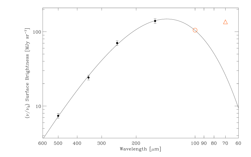
Figure 1.— Representative SED in the Orion A map. The derived temperature is 17.9 K and the optical depth at 250 µm is 6.3$\times 10^{-4}$. Only the four lowest frequency Herschel passbands were used in fitting the modified blackbody SED. This model predicts the 100 µm IRAS brightness quite well (open circle, see Appendix B) but underpredicts the 70 µm emission (triangle) where non-equilibrium emission from VSGs becomes important.

The IRAS 100 µm brightness was used in fitting SEDs in previous work (Planck Collaboration et al., 2011a; Martin et al., 2012), but was not included here because of its relatively low angular resolution ($\sim 4$$\farcm$3). As discussed in Appendix B, we subsequently checked that the 100 µm emission is consistent with the SED fit. On the other hand, the 70 µm emission is greater than that predicted by the equilibrium emission SED, confirming the additional contribution from VSGs (see example in Figure 1).

Errors on the parameters from the SED fit were estimated using Monte Carlo simulations after assessing the various sources of error in the intensities of the Herschel images (see Appendix C). A typical SED fit has a $\chi^{2}$ near two (as expected for four intensities, two parameters, and thus two degrees of freedom) and the map of $\chi^{2}$ is featureless.

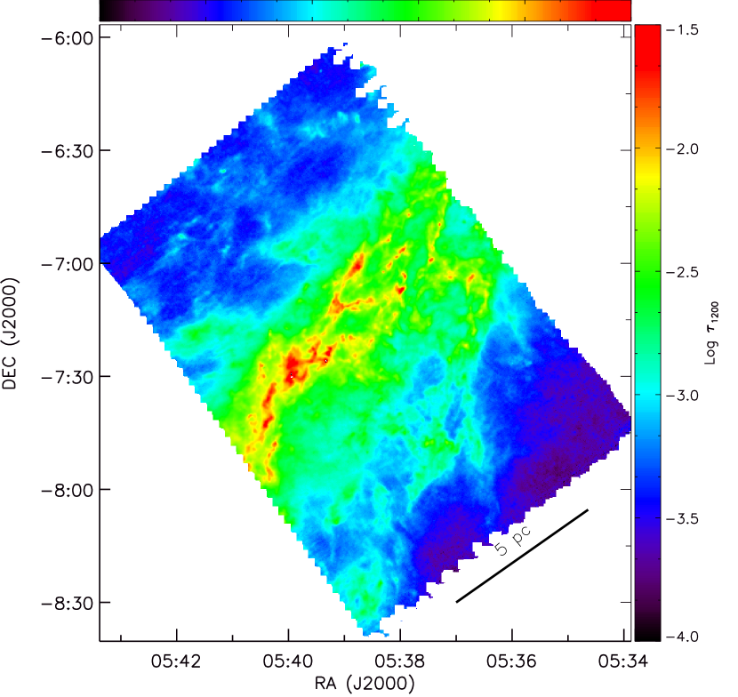
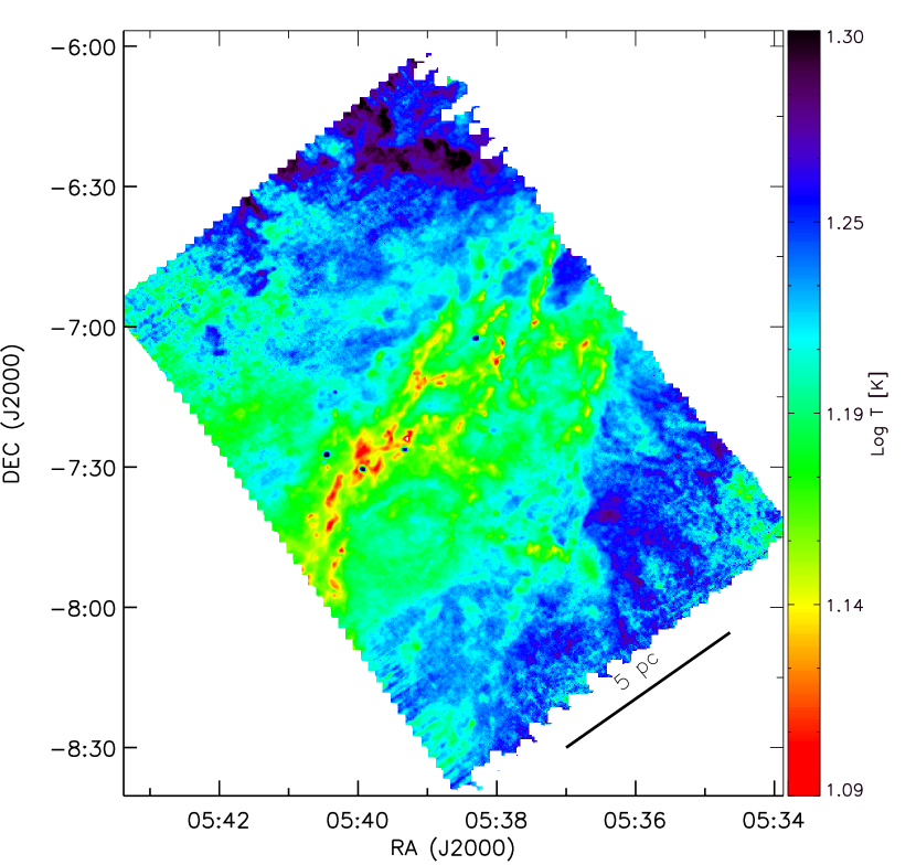
Figure 2.— Left: Optical depth map for Orion A-C1 as obtained from fitting SEDs to the 160-µm PACS and three SPIRE intensities, from images brought to a common resolution of 37$\farcs$0. The dust emissivity index $\beta$ was fixed at 1.8. Right: Corresponding temperature map, with a complementary inverted color scale. The logarithmic range spans 12.3 to 20.0 K. Note by comparison with the optical depth how the dust in regions of high column density tends to be cooler ($<1.14$ dex or 13.8 K) than in diffuse low column density regions ($>1.23$ dex or 17 K). Within the cool filaments are a few compact regions where the dust is heated by embedded protostars. The few more diffuse regions with low column density but even higher dust temperature have an enhanced local radiation field; see also Figure 6 in Section 5.2 below.

Figure 2 shows results from the SED fits as maps of the fitting parameters for the Orion A-C1 field. The left panel shows a map of $\tau_{1200}$; the variation of $N_{\rm H}$ is shown by the top color bar, adopting the mean relation found below (Figure 3). The corresponding map of $T$ is in the right panel; a complementary inverted logarithmic scale has been used to bring out both the general anti-correlation (see also Figure 5 in Section 5.1) and exceptions. One common feature in these two maps of the fitting parameters is the filamentary structure, which is of high column density and generally low temperature, as might be expected for an IRSF that is attenuated in those regions. This behavior is discussed further in Section 5. Filaments are common in the HGBS (André et al., 2010; Men’shchikov et al., 2010; Arzoumanian et al., 2011; Peretto et al., 2012), HOBYS (Motte et al., 2010; Hill et al., 2011; Hennemann et al., 2012; Schneider et al., 2012), and Hi-GAL (Molinari et al., 2010) images.

4. Submillimeter Optical Depth, $N_{\rm H}$, and Opacity

4.1. $\tau$ and $N_{\rm H}$

Before comparison with our $E(J-K_{\rm s})$ proxy for $N_{\rm H}$, all parameters resulting from the SED fits on the Herschel maps were sampled to match the map of $E(J-K_{\rm s})$ (Appendix A.3). Figure 3 shows a plot of the sampled $\tau_{1200}$ against $N_{\rm H}$ from the conversion from $E(J-K_{\rm s})$ in Equation (A1).

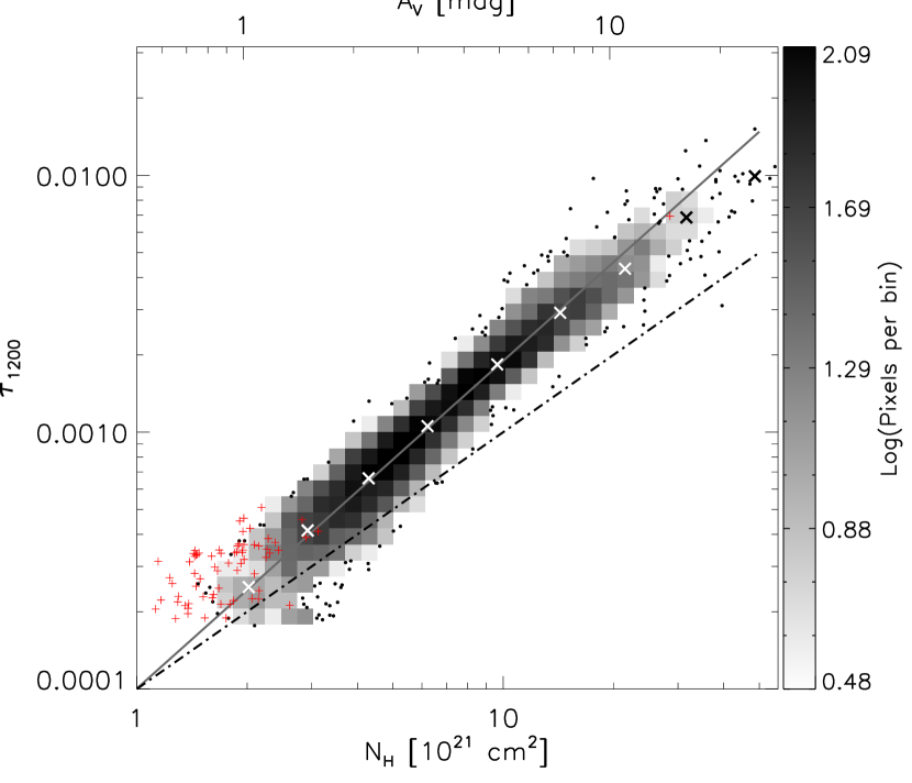
Figure 3.— $\tau_{1200}$ from SED fits versus column density $N_{\rm H}$ obtained from near-infrared color excess $E(J-K_{\rm s})$. Given the large number of pixels in the maps, we have used a logarithmic grey-scale to represent different values in a two-dimensional histogram of the number of pixels per bin. Individual data points are plotted (dots) where the density of points is low, less than or equal to three. Data where $N_{\rm H}$ has $S/N<2$ are plotted as red pluses and are not included in the histogram or fit; these are also identified in subsequent figures. The crosses show data binned logarithmically along $N_{\rm H}$. The dotted-dashed line shows a linear relationship between $\tau_{1200}$ and the underlying $N_{\rm H}$ based on a fixed dust opacity, here $\sigma_{\rm e}(1200)=1\,\times 10^{-25}$ cm² H^-1 typical of high latitude dust. Compared to this relation there appears to be a non-linear increase in $\tau_{1200}$ (and thus $\sigma_{\rm e}$(1200)) with $N_{\rm H}$. The solid line is the power-law correlation obtained from fitting $\tau$ and $N_{\rm H}$, excluding the low $S/N$ data. The fit yields a power law index $1.28\pm 0.01$ (slope of the line) and amplitude $(1.01\pm 0.02)\times 10^{-4}$ for the adopted units (intercept at $N_{\rm{H}}=10^{21}$ cm^-2).

The two independent measures of column density are well correlated. The data have some dispersion, with possible reasons including uncertainty in the measurement of color excess, cosmic scatter about Equation (A1) converting $E(J-K_{\rm s})$ to $N_{\rm H}$, and errors in the determination of $\tau_{1200}$ from the SED.

Observationally, the properties of dust grains have been best constrained for the high latitude diffuse ISM. For example, the equilibrium dust temperature is typically near 18 K and $\sigma_{\rm e}$(1200) is $1.0\times 10^{-25}{\rm cm^{-2}}~{}\rm H^{-1}$ (Boulanger et al., 1996; Planck Collaboration et al., 2011a). The expected linear relation for this opacity is plotted with the dotted-dashed line in Figure 3. This relation is close to that of the present data at low column density. However, there appears to be a significant non-linearity in the data. The formal fit, excluding $N_{\rm H}$ data with $S/N<2$, is $\tau_{1200}\propto N_{\rm H}^{1.28\pm 0.01}$; the systematic error on the index is 0.03. Such non-linearity appears to be evidence for grain evolution.

Recall that $\tau_{1200}$ was derived under the assumption of a constant $\beta$. We also derived $\tau_{1200}$ treating $\beta$ as a (third) free parameter, in case $\beta$ evolves too. However, we found that $\beta$ does not change systematically with column density, and so the same non-linear trend is observed in Figure 3 – the evidence for grain evolution remains. There is increased scatter about the mean correlation and the intercept is 10% higher because the average $\beta$ is 1.96 (with higher $\beta$, SED fits tend to have lower $T$ and hence higher $\tau$).

Although the conversion factor from $E(J-K_{\rm s})$ to $N_{\rm H}$ might not be constant for the higher $N_{\rm H}$ in Figure 3, there is already some divergent non-linear behavior within the range $N_{\rm H}$$<5\times 10^{21}$ cm^-2 that is calibrated (Martin et al., 2012) . Nevertheless, we have to be aware that apparent non-linearity might simply be a reflex of an erroneous conversion of $E(J-K_{\rm s})$ to $N_{\rm H}$ (see Equation (A1)). To remove the evidence for grain evolution, i.e., to maintain a constant submillimeter opacity, would require $N_{\rm H}\propto E(J-K_{\rm s})^{1.28}$ – which would itself be evidence for grain evolution, albeit as it affects the near-infrared extinction. This dependence, is however, opposite to what has been predicted for the initial changes in extinction curves resulting from grain evolution by ice-mantle formation and aggregation (Ormel et al., 2011).

Furthermore, empirically, the ratio of $E(J-H)$/$E(H-K_{\rm s})$ is constant with column density (Appendix A.1). Chapman & Mundy (2009) find the same constancy in the shape of the near-infrared extinction curve in probes of cores to slightly higher peak optical depth than reached here, but interestingly they find an increase in the relative amount of mid-infrared extinction at high optical depth. A constant shape of the near-infrared extinction curve, despite changes in the visible (e.g., as encoded by $R_{V}$), would be consistent with aggregation of the smallest interstellar grains with the largest, but not with aggregation among the largest particles, because in the latter case the scattering would be greatly enhanced contributing to a steeper wavelength dependence (Kim et al., 1994). The enhanced mid-infrared extinction seen at high column densities might be explained by the addition of ice mantles (Chapman & Mundy, 2009). Possibly the same affects the submillimeter. Grain evolution, when and where it occurs, might be complex and different than this and so it is hard to be definitive. Until there is evidence to the contrary, we think it is reasonable to adopt $E(J-K_{\rm s})$ as a measure of $N_{\rm H}$ over the range of column densities found in this field, and thus we conclude that it is the submillimeter opacity that has changed. But it remains important to understand how the submillimeter opacity can change without a noticeable change in the near infrared.

Dense filaments appear to have a characteristic linear width $\sim 0.1$ pc (Arzoumanian et al., 2011; Fischera & Martin, 2012b) which is 50″ at the $\sim 400$ pc distance of Orion. This scale is not much larger than the 37″ resolution of our Herschel maps of $\tau_{1200}$ but is significantly smaller than the $\sim 3\farcm 5$ resolution of the $E(J-K_{\rm s})$ map (Appendix A.2) required for our opacity study. Therefore, we do not have enough spatial resolution to investigate in detail the opacity of dust inside individual filaments (or prestellar cores) where the column density and volume density would be even higher. We are not able to see if the trend indicating grain evolution continues to even higher densities. But see the brief discussion ending the next subsection.

The highest column densities ($A_{\rm V}>8$) are the most likely to have been influenced by self gravity. In principle, if extremely compact structures developed there and had a low covering factor they might be missed in the ‘AvMAP’ assessment of $E(J-K_{\rm s})$ because of the relatively sparse sampling by the 2MASS stars (Appendix A.1), and yet they would still contribute to the Herschel assessment of $\tau_{1200}$ because their emission would be included in the finite beam. If that were the case and if such structures had a significant column density, then the $N_{\rm H}$ derived from $E(J-K_{\rm s})$ would be underestimated relative to the sampled $\tau_{1200}$, and so the observed trend in Figure 3 would turn up above this high column density. If anything, the data there fall slightly below the non-linear dependence shown. This mapped region of the molecular cloud does have some compact (self-gravitating and probably quasi-equilibrium) high column density structures, filaments and even some ‘cores,’ with enough mass to be detectable in the submillimeter, but their physical size is large enough that at the distance to the Orion A cloud these structures are measured to be resolved, and so are not as in our hypothetical scenario physically vanishingly small and not sampled by the 2MASS stars. Another constraint on any hypothesis aiming to account for, or explain away, this non-linearity is that the trend in Figure 3 begins at quite low column densities. Furthermore, there is ample evidence for a higher opacity associated with high column density molecular regions (see, e.g., the summary in Appendix A in Martin et al., 2012, and the following subsection).

4.2. Opacity $\sigma_{\rm e}(1200)$ and $N_{\rm H}$

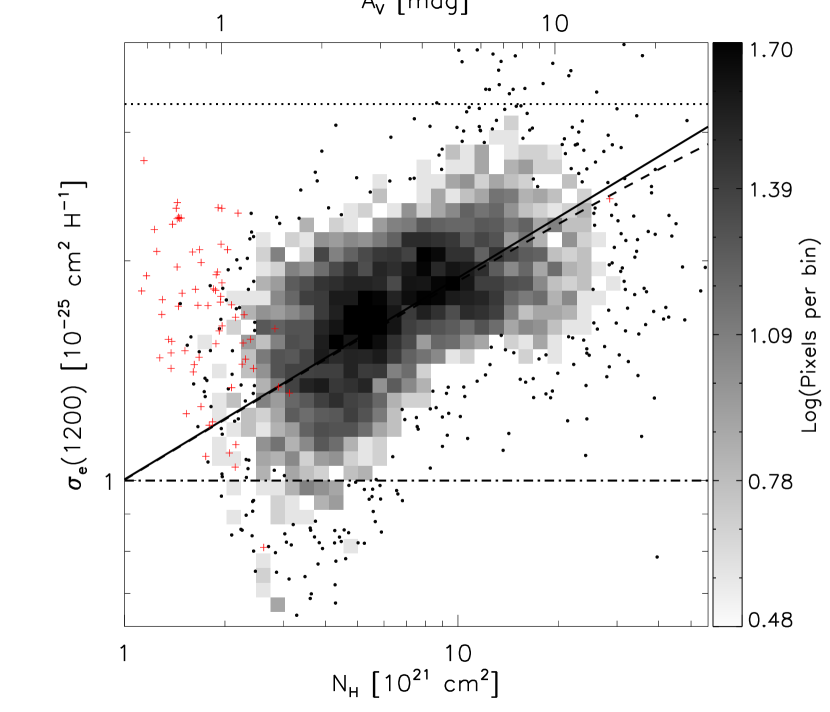
Figure 4.— Opacity $\sigma_{\rm e}$(1200) versus $N_{\rm H}$. The solid line shows a power-law variation $\sigma_{\rm e}$(1200) $\propto$ $N_{\rm H}$^0.28 taken from the solid line in Figure 3. The dashed line depicts the effect of color correction due to the finite bandwidth of the 2MASS filters on the measurement of $E(J-K_{\rm s})$ (column density). The horizontal dotted-dashed line shows the average $\sigma_{\rm e}$(1200) for the diffuse ISM. The dotted line is for $\sigma_{\rm e}(1200)=3.3\,\times 10^{-25}$ cm² H^-1, the standard adopted by the HGBS and HOBYS. Pixels representing two-dimensional histogram is same as described in Figure 3. Individual data points are plotted where the density of points is less than or equal to three.

The nature of the systematic change in $\sigma_{\rm e}$(1200) is revealed more explicitly in Figure 4, which is just an alternative representation of Figure 3, from the sampled $\tau_{1200}$ map simply divided by the $N_{\rm H}$ map, plotted on an expanded vertical scale. The solid and dotted-dashed lines are the same as defined for Figure 3. Despite the dispersion about the solid line, the overall trend clearly indicates an increase of $\sigma_{\rm e}(1200)$ with column density ($\sigma_{\rm e}(1200)\propto N_{\rm H}^{0.28\pm 0.01\pm 0.03}$), by at least a factor of two over this $N_{\rm H}$ range.

A particular additional perspective provided by the present study of this region in Orion A is that there ought to be a rough correspondence between volume density and column density. This link could enable a more direct connection of grain evolution to environment. Compared to the density of the diffuse ISM ($n_{\rm H}\sim 1$ – 10 cm^-3), the density typical of a star formation region where clumps are beginning to show signs of gravitational contraction is several orders of magnitude higher (10³ – 10⁵ cm^-3). In the present analysis, we are probing environments, especially in filamentary structures, with $n_{\rm H}$ up to $\sim 10^{4}$ cm^-3.

The measurement of $\sigma_{\rm e}$(1200) is sensitive to the estimate of temperature through the Planck function; see Equation (1) where we have assumed a constant $T$ along the line of sight. Obviously, either for passively-heated molecular clouds with significant optical attenuation or for those with an internal energy source, there is a gradient in temperature which we have ignored. Particularly relevant here is the former possibility which has been studied extensively using radiative transfer simulations. For example, Ysard et al. (2012) found that the temperature obtained from fitting a single-temperature SED is overestimated compared to the true dust temperature for central lines of sight through filaments or spherical clouds. The difference increases non-linearly with central column density and is noticeable by $N_{\rm{H}}\sim 14\times 10^{21}$ cm^-2, depending on the grain model. In the context of our analysis, an ‘overestimate’ of the temperature would have suppressed the optical depth derived here; hence, this effect would enhance rather than erase the trend of increasing $\sigma_{\rm e}$(1200) with $N_{\rm H}$.

The dashed line in Figure 4 shows the correction of the correlation line when the effect of the finite filter bandwidths on the color excess is taken into account (see Appendix A.5). Underestimation of $E(J-K_{\rm s})$ makes the rate of increase in $\sigma_{\rm e}$(1200) only marginally smaller.

For the pixels with low column density, the derived values of $\sigma_{\rm e}$(1200) are close to the value $1\times 10^{-25}$ cm² H^-1 for high latitude diffuse interstellar dust (Boulanger et al., 1996) and typically within the range of $(0.6-1.6)\times 10^{-25}$ cm² H^-1 found by Planck Collaboration et al. (2011a). We find that $\sigma_{\rm e}$(1200) increases systematically with $N_{\rm H}$ by at least a factor two. Such high opacities are not unprecedented, one example being $3.8\times 10^{-25}$ cm² H^-1 for a dense molecular region in the Vela molecular ridge where the column density ranged between 10 to $40\times 10^{21}$ cm^-2 (Martin et al., 2012). For a molecular region in Taurus of intermediate column density ($\sim 10^{22}$ cm^-2), Planck Collaboration et al. (2011b) obtained an opacity of $(2.3\pm 0.3)\times 10^{-25}$ cm² H^-1. By contrast, for the neighboring atomic phase with $N_{\rm{H}}<3\times 10^{21}$ cm^-2, they obtained $(1.14\pm 0.2)\times 10^{-25}$ cm² H^-1. Based on a complementary new method, physical modeling of the brightness profiles of filaments, Fischera & Martin (2012a) find a range $(1.3-2.8)\times 10^{-25}$ cm² H^-1 (the range depending on the adopted distance). These are consistent with the trend seen in Figure 4.

The standard opacity adopted by the HGBS and HOBYS (e.g., André et al., 2010; Motte et al., 2010) is $\sigma_{\rm e}(1200)=3.3\,\times 10^{-25}$ cm² H^-1 (see Figure 4). This is taken from theoretical calculations by Preibisch et al. (1993) for evolved dust in protostellar cores (see also Ossenkopf & Henning, 1994). Although we do not probe to such high densities, this value seems a reasonable extrapolation of the trend in Figures 3 and 4; a corollary is that a single value of the opacity cannot be used for all environments across a region.

As emphasized by Shirley et al. (2011), the largest uncertainty in determining the mass of a core is in the adopted value of the opacity. Their modeling of the extended submillimeter emission in the cold envelope of B335, combined with deep imaging at $H$ and $K$ ($E(H-K)$ up to 3, about three times larger than in our map), allowed them to constrain the ratio of the submillimeter opacity, at 850 µm, to the opacity (scattering plus absorption) at 2.2 µm. They found a range $(3.2-4.8)\times 10^{-4}$. Extrapolating this to the ratio involving the opacity at 250 µm using their estimate of $\beta$ (2.18 to 2.58) gives a range $(4.6-11.3)\times 10^{-3}$. This can be compared to our estimate of the same ratio, $(2.3-4.9)\times 10^{-3}$ for $\sigma_{\rm e}(1200)=(1-2)\times 10^{-25}$ cm² H^-1 (note that this ratio is independent of the calibration of either opacity to $N_{\rm H}$). Thus regions characterized by higher density, or higher column density here, both appear to have an enhanced submillimeter opacity relative to that in the $K$ band (and one cannot rule out that both might have increased). Of course, as we have noted in the Introduction, what is really needed to find the mass is the product $r\kappa_{\nu}$, and so without some direct calibration as attempted here, the Achilles heel is to first derive the submillimeter dust opacity itself from the above opacity ratio and then adopt an appropriate dust to gas ratio $r$.

5. Power

Big dust grains bathed in the ISRF absorb energy at higher frequencies, and in thermal equilibrium they re-emit the same amount of energy at much lower frequencies. Thus, the observed $P$ is what the grains were able to absorb in their environment, per H. For the dust emissivity relation ($\beta$) adopted, $P$ can be expressed as

$$P/P_{0}=(\sigma_{\rm e}(1200)/\sigma_{0})\,(T/T_{0})^{5.8},$$ (3)

normalized in terms of the average parameters in the diffuse atomic ISM at high latitude (Planck Collaboration et al., 2011a): $T_{0}=17.9$ K, $\sigma_{0}=1.0\times 10^{-25}$ cm² H^-1 and $P_{0}=3.8\times 10^{-31}$ W H^-1.

5.1. $T$ and $\tau$

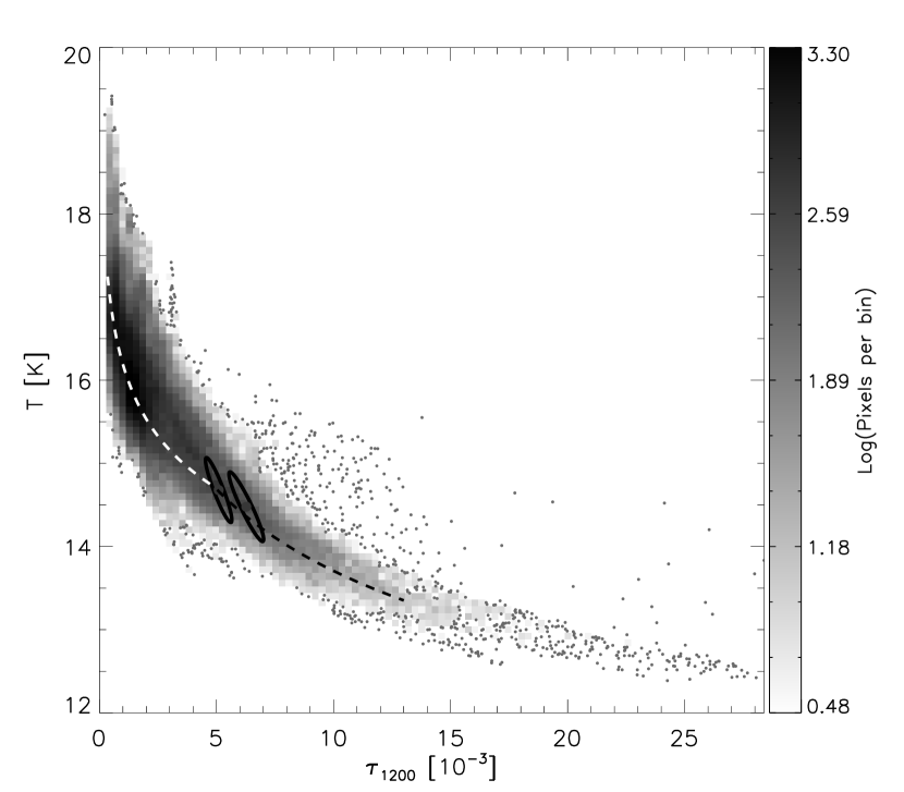
Figure 5.— $T$ versus $\tau_{1200}$ from the SED fits, with the logarithmic grey-scale representing the values in a two-dimensional histogram. Representative error ellipses for a single pixel are from Monte Carlo simulations of the SED fitting. The dashed curves are power laws schematically following the anti-correlation. Individual data points are plotted where the density of points is less than or equal to three.

The value of the equilibrium grain temperature is not a primary dust parameter. Rather, as is clear from Equation (3), $T$ is a parameter that responds to environmental changes in the ISRF affecting the absorbed $P$ and to changes in the grain properties like $\sigma_{\rm e}$(1200) and possibly the absorption which also affects the absorbed $P$.

The anti-correlation of $T$ and $\tau_{1200}$ seen in the maps of Figure 2 and similarly for the Orion A-S1 field is highlighted in Figure 5. Because we are primarily interested in regions where there is no internal source of energy, we have not plotted data for the pixels corresponding to a few identified embedded protostars (high $T$ and intermediate $\tau_{1200}$). The dashed curves are not a fit but rather trace the general trend schematically. We have transferred these loci to Figures 7 - 9 below to gain insight into relationships between other variables. For simplicity, we have used two power laws, $T/T_{\rm b}=(\tau(1200)/\tau_{\rm b})^{-\alpha}$, where a break occurs at $T_{\rm b}=14.7$ K and $\tau_{\rm b}=4.9\times 10^{-3}$, and where $\alpha=0.06$ and 0.1 below and above the break, respectively.

5.2. Spatial Dependence of $P$

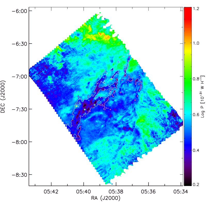
Figure 6.— Map of the specific power $P$ in the Orion A-C1 field. The overplotted white contour, corresponding to $N_{\rm H}=20\times 10^{21}$ cm^-2 ($A_{V}$ $\sim 10.6$ mag), reveals how $P$ decreases significantly in high column density regions, especially here along filaments.

We produced a map of $P$ shown in Figure 6 making use of the $T$ and $\tau$ maps (as in Figure 2) and the average dependence of $\sigma_{\rm e}$(1200) on $\tau_{1200}$ from Figures 3 and 4. More directly from the data, a map of the radiated energy is obtained from the integration of the respective SEDs over all frequencies. As in Section 4.2, we divide the resulting sampled map by the $N_{\rm H}$ map to obtain a map of the specific power $P$ (Equation (2)). This is very similar to Figure 6.

For the pixels corresponding to low $N_{\rm H}$, $P$ is on average about 3.7$\times 10^{-31}$ W H^-1, close to the value $3.8\times 10^{-31}$ W H^-1 for the typical specific power in the diffuse ISM at high Galactic latitude (Planck Collaboration et al., 2011a). In a few diffuse regions in our maps, for example the northern part of Orion A-C1, $P$ gets as high as $10\times 10^{-31}$ W H^-1, clearly showing an enhancement of the local radiation field by a factor of $\sim 2.5$ times relative to the average ISRF. Others examples are the B77 Bright Nebula and a halo around V1792 Ori, both in the Orion A-S1 field and so not shown here. These regions also have strong emission at 70 µm and 160 µm in the respective Herschel images.

As illustrated in Figure 6 by the overlay of the contour $N_{\rm H}=20\times 10^{21}$ cm^-2, regions with the highest $N_{\rm H}$ tend to have lower $P$. The most straightforward qualitative interpretation is in terms of attenuation of the ISRF. The high frequency components of the ISRF that are primarily responsible for the heating of the dust grains cannot penetrate easily into the interior of the denser molecular structures. Most of the power is absorbed within the outer layers of the cloud and so the dust in the core generally has a lower equilibrium temperature.

It should be noted that only a fraction of the total $N_{\rm H}$ through the center of the filaments is associated directly with the structure, the rest arising from the embedding and foreground and background material. Therefore, the detailed relationship between specific power and column density requires knowledge of density profiles and cloud geometry, the strength of the ambient ISRF, and detailed radiative transfer modeling taking into account appropriate dust populations and absorption and scattering properties (Fischera, 2011; Ysard et al., 2012).

In contrast, and not surprisingly, close inspection of Figure 6 reveals a few lines of sight where there is an internal source of energy (protostar(s)) within a dense compact structure. With this extra energy input, the resulting $P$ is higher locally. These are readily seen in Figure 2 (right) as warmer than the immediate surroundings. An example is at $RA,Dec$ 05:39:56, $-$7:30:27, in a complex environment with the brightest hot source named LDN 1641 S3 IRS/ FIRSSE 101.

5.3. $P$ and $N_{\rm H}$

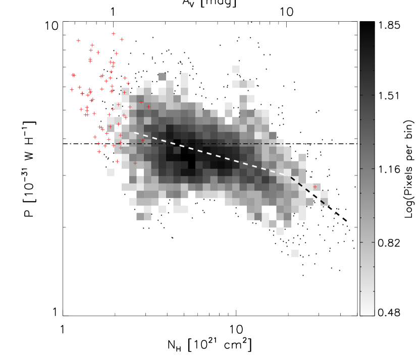
Figure 7.— Specific power $P$ versus column density $N_{\rm H}$. $P$ fluctuates about the typical high latitude diffuse ISM value of 3.8 $\times 10^{-31}$ W H^-1 (dotted-dashed line). For high column density, $P$ decreases because of attenuation of the ISRF. Dashed lines show the loci transferred combining trends from Figures 3 - 5. Pixels representing two-dimensional histogram is same as described in Figure 3. Individual data points are plotted where the density of points is less than or equal to three.

Figure 7 shows the relationship of sampled $P$ to $N_{\rm H}$. There is a trend of decreasing $P$ at higher column density that sets in well before the value $20\times 10^{21}$ cm^-2 emphasized in Figure 6. Above we quantified trends relating $\sigma_{\rm e}$(1200) and $\tau_{1200}$ to $N_{\rm H}$, and $T$ to $\tau_{1200}$. If we substitute these trends in Equation (3), we find $P/P_{\rm b}=(N_{\rm H}/N_{{\rm H}_{b}})^{-\delta}$, where $P_{\rm b}=2.98\times 10^{-31}$ W H^-1 and $N_{{\rm H}_{\rm b}}=20.3\times 10^{21}$ cm^-2, and where $\delta=0.165$ and 0.46 below and above the break, respectively. These loci are plotted in Figure 7.

6. Interrelationships among $T$, $P$, and $\sigma_{\rm e}$(1200)

Among $T$, $P$, and $\sigma_{\rm e}$(1200), a scatter plot of any two provides insight into their interrelationship. On the resulting figures, we also plot loci defined by fixing the third quantity.

6.1. $T$ – $\sigma_{\rm e}$(1200) Relation

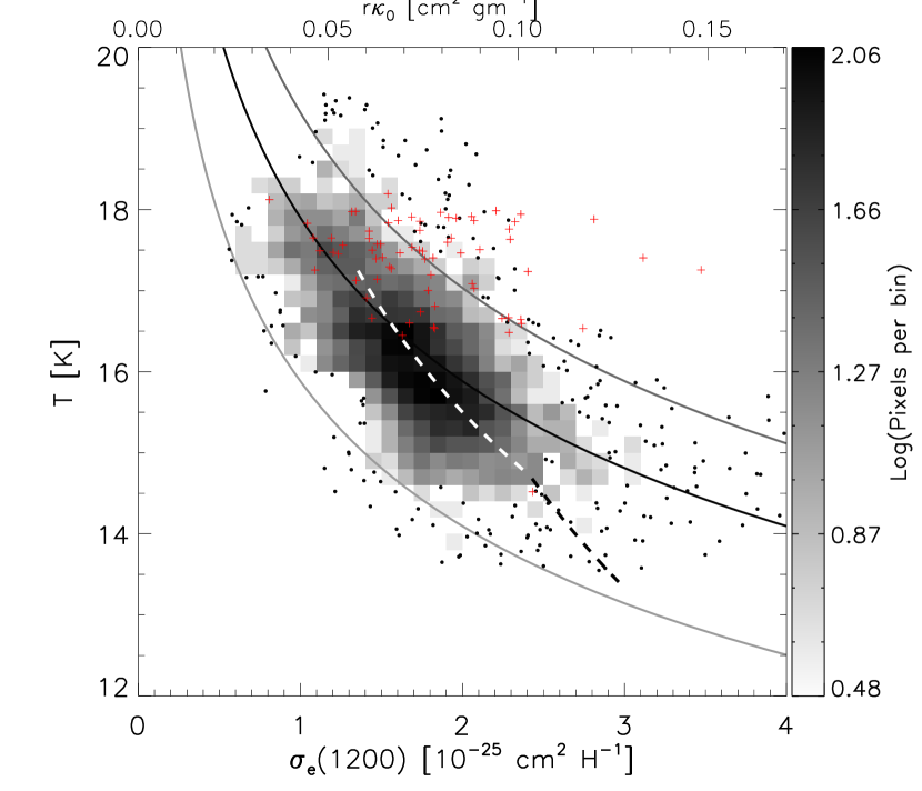
Figure 8.— Dust temperature $T$ versus dust opacity $\sigma_{\rm e}$(1200). Solid lines are the loci of constant specific power, $P$. The middle line is for 3.8 $\times 10^{-31}$ W H^-1, the typical $P$ in the high latitude mean ISRF (see Section 5). The lower and upper lines are for an ISRF different by factors of 0.5 and 1.5, respectively. Dashed lines show the loci transferred combining trends from Figures 3 - 5. Pixels representing two-dimensional histogram is same as described in Figure 3. Individual data points are plotted where the density of points is less than or equal to three.

As discussed above, the dust temperature is determined by the energy balance between the power absorbed from the ISRF and emission. For a given intensity of the ISRF and absorption coefficient, and thus absorbed power, grains with a higher $\sigma_{\rm e}$(1200) radiate more efficiently and so attain a lower equilibrium temperature (Equation 3). Therefore, the observed equilibrium dust temperature and the intrinsic dust property $\sigma_{\rm e}$(1200) are expected to be inversely related. In Figure 8, we show the anti-correlation between sampled $T$ and $\sigma_{\rm e}$(1200) for the Orion A region. The solid line shows a locus of constant specific power $P=3.8\times 10^{-31}$ W H^-1 whereas the loci below and above are 0.5 and 1.5 times this value, respectively. There is a range of $P$ and indeed, unlike in the high latitude diffuse ISM, we do not expect to have constant $P$ in the regions of high column and volume density (see Figure 7), due to attenuation by dust itself. To capture this effect, we have transferred the loci from the above figures. We find $T/T_{\rm b}=(\sigma_{e}(1200)/\sigma_{b})^{-\epsilon}$, where $\sigma_{\rm b}=2.41\times 10^{-25}$ cm² H^-1 and where $\epsilon=0.27$ and 0.46 below and above the break, respectively. These loci are plotted in Figure 8.

6.2. $P$ – $\sigma_{\rm e}$(1200) Relation

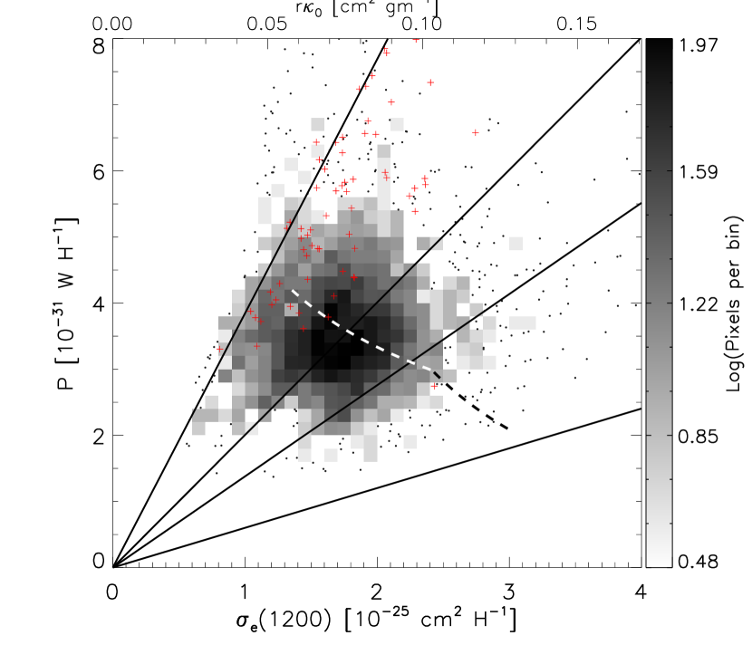
Figure 9.— Specific power $P$ versus dust opacity $\sigma_{\rm e}$(1200). The solid lines (bottom to top) are the loci of constant temperatures equal to 13, 14, 15, and 17.9 K. Dashed lines show the loci transferred combining trends from Figures 3 - 5. Pixels representing two-dimensional histogram is same as described in Figure 3. Individual data points are plotted where the density of points is less than or equal to three.

Figure 9 shows sampled $P$ versus $\sigma_{\rm e}$(1200), and is sufficient to complete our examination of the three-parameter relations of Equation (3) ($P$ versus $T$ being redundant). For a given dust equilibrium temperature, the power radiated in the submillimeter is proportional to the emission cross-section. The solid lines are the loci of constant temperature with increasing slope corresponding to 13, 14, 15, and 17.9 K, respectively. For dust grains exposed to same ISRF (constant $P$), the less efficient emitters (lower $\sigma_{\rm e}$(1200)) will have higher temperature.

To capture the effect of attenuation, we have transferred the loci from the previous figures. We find $P/P_{\rm b}=(\sigma_{\rm e}(1200)/\sigma_{\rm b})^{-\iota}$, where $\iota=0.59$ and 1.65 below and above the break, respectively. These loci are plotted in Figure 9.

7. Conclusion

We have studied the properties of dust grains using multi-wavelength images of thermal dust emission in the Orion A molecular cloud at 160, 250, 350, and 500 µm, acquired by the PACS and SPIRE cameras on Herschel as part of the HGBS. We fit a modified blackbody model to the spectral dependence of the surface brightness of each pixel. Although dust along the line of sight is probably not all at the same temperature, assuming a single $T$ is a reasonable model providing good quality SED fits to the Herschel data. Thus, we obtained the spatial distribution of $T$ and $\tau_{1200}$ across the map.

The derived optical depth map is well correlated with the $N_{\rm H}$ map derived from $E(J-K_{\rm s})$ and we combined them to explore how the dust opacity $\sigma_{\rm e}$(1200) varies with column density. A submillimeter opacity $\sigma_{\rm e}$(1200) near $1\times 10^{-25}$ cm² H^-1 is typical for diffuse dust along high latitude lines of sight of low column density ($A_{V}$$\sim$ 1 mag) and close to that found at low column density in these Orion A fields. On lines of sight intercepting high column density filamentary structures, however, we found evidence for an increase of $\sigma_{\rm e}$(1200) by a factor two or more, approaching that adopted by the HGBS and HOBYS. Overall, there is a systematic trend $\sigma_{\rm e}(1200)\propto N_{\rm H}^{0.28}$. This dependence is strong evidence for grain evolution with environment. There is not a single opacity that can be applied to a whole mapped region with environments ranging from diffuse to higher column density structures. This has quantitative implications for the interpretation of the probability distribution function of the column density and possibly for the shape of the core mass function.

For the low column density lines of sight, the average value for the specific power $P$ is $3.7\times 10^{-31}$ W H^-1, equivalent to 1.2 $L_{\odot}$/$M_{\odot}$. The power emitted is equal to the power absorbed and so depends on the local ambient ISRF. Thus, the decrease of $P$ that we see in the dense filamentary structures ($P\sim 1.5\times 10^{-31}$ W H^-1) can be attributed to attenuation of the ISRF. There are also local enhancements of the ISRF. Overall, $P$ ranges over a factor of 10, roughly centered on the diffuse ISM value.

The emission opacity $\sigma_{\rm e}$(1200) of big grains together with the relative strength of the ISRF determines the equilibrium temperature. In the diffuse ISM where dust grains are exposed fully to the ISRF, the temperature is typically 18 K. Inside dense filamentary structures in the observed region of the Orion A molecular cloud, the opacity is larger and the ISRF is attenuated, both leading to dust temperatures lower than 14 K.

In this high latitude region in the Orion A molecular cloud, high column density arguably corresponds to high volume density. The observed change in the optical properties of dust grains in dense cold regions can be attributed to grain growth due to aggregation and/or accretion of ice mantles. This process might reasonably be expected to correlate with a decrease in the relative abundance of VSGs. It is difficult, however, to probe the presence of the latter because the radiation that would normally excite their non-equilibrium emission at shorter wavelengths ($<$ 100 µm) is sharply attenuated in these very regions.

Appendix A 2MASS Color Excess and Column Density

Column density can be estimated by measuring extinction or color excess. Very productive use has been made of the near-infrared 2MASS data in the J, H, and ${\rm K_{s}}$ passbands, post-processed by a variety of techniques (e.g., Rowles & Froebrich, 2009; Dobashi, 2011; Lombardi et al., 2011). To stay close to the data and avoid unnecessary additional assumptions (see also Appendix A.4), here we quantify the extinction in terms of the near-infrared color excess $E(J-K_{\rm s})$, rather than the total visual extinction $A_{\rm V}$. For comparison to values cited in other literature, the adopted conversion has been $A_{\rm V}=5.89\,E(J-K_{\rm s})$.

A.1. Sampling the Color Excess

The extinction map was derived using the ‘AvMAP’ procedure (Schneider et al., 2011) as a weighted average of measures of $E(J-H)$ and $E(H-K_{\rm s})$, and subsequently expressed here as $E(J-K_{\rm s})$. The map is created from a weighted mean of the color excesses of individual stars. The weighting function is a Gaussian of $FWHM=4\arcmin$ centered on each $2\arcmin$ pixel and stars are considered out to a radius of $3\,\sigma$ ($1.3\,FWHM$). To monitor the quality, maps of the weighted number of stars used and the weighted standard deviation of the mean (i.e., the uncertainty of $E(J-K_{\rm s})$) are also computed.

Given the high column densities reached in this field, the issue arises whether the color excess maps might somehow be ‘saturated,’ i.e., missing the highest values. This issue does not seem to be addressed in the literature. We have made scatter plots of the maps of Rowles & Froebrich (2009) and Dobashi (2011) compared to our $E(J-K_{\rm s})$ map. These plots show good correlations with the expected slope up to $A_{\rm V}\sim 8$, after which these other products cease to continue to rise as our $E(J-K_{\rm s})$ grows further.

Maps of $E(J-H)$ and $E(H-K_{\rm s})$ can be derived separately. These correlate very well with a slope of $1.73\pm 0.01$, close to the ‘normal’ value 1.7 (see discussion in Martin et al., 2012). Like Lombardi et al. (2011) have also shown for the Orion A cloud, this normal color-color relation extends beyond $E(J-H)=1.7$ mag and $E(H-K_{\rm s})=1$ mag, though the correlation becomes noisier. Thus, there seems to be no evidence for either the effects of grain evolution or of saturation of one color with respect to the other up to $E(J-K_{\rm s})=2.7$ mag which corresponds to $A_{\rm V}\sim 16$ mag. Nevertheless, we need to acknowledge the issue and ensure that the column density from Herschel $\tau$ is sampled on a closely comparable basis. This is accomplished as described in Appendix A.3.

A.2. Gauging the Resolution

In our Herschel maps of $\tau_{1200}$ at 37″ resolution there is structure on smaller scales than the $4\arcmin$ weighting function of ‘AvMAP.’ Therefore, it is important that the map of $\tau_{1200}$ be brought to the lower resolution of the $E(J-K_{\rm s})$ map for an unbiased comparison (Section 4.1). Establishing the precise resolution of color excess maps derived from 2MASS data has not been a high priority and so we have done our own explorations. A fruitful approach was to use the power spectrum of the map. A traditional map (image) produced by an instrument with a ‘beam’ (or point spread function) is typically oversampled relative to the beam size and so the information in neighboring pixels is correlated. Therefore, there is a predictable roll-over of the power spectrum at high spatial frequencies corresponding to the size of the beam. Although the described Gaussian-weighted and truncated sampling used in ‘AvMAP’ is not exactly convolution, nonetheless we found an empirical roll-over of the power spectrum that can be described quantitatively by a beam of $FWHM$ 3$\farcm$5, which seems reasonable.

A.3. Sampling the Herschel  $\tau_{1200}$ map

Ideally, the two independent measures of column density, $E(J-K_{\rm s})$ and $\tau_{1200}$, would sample the sky in the same way. Rather than trying to bring the higher resolution $\tau_{1200}$ map to the lower effective resolution of the $E(J-K_{\rm s})$ map by smoothing, a more direct approach is to sample the $\tau_{1200}$ map at the positions of 2MASS stars, forming the weighted average in the same way as in ‘AvMAP.’ We found that simply extracting cataloged 2MASS stars according to the criterion of photometric $S/N>7$ produced a weighted number of stars close to ‘AvMAP.’ While this is not precisely an identical sampling, nor is the original $\tau_{1200}$ known to pencil-beam precision. Thus we obtain a map of $\tau_{1200}$ on the same pixels as for $E(J-K_{\rm s})$ and with comparable sampling of the column density and resolution pixel by pixel. Quantitatively, there is a roll-over in the power spectrum of the sampled $\tau_{1200}$ map for each of the two Herschel fields that confirms a typical resolution 3$\farcm$5.

A.4. Calibration of the Column Density

Martin et al. (2012) made a direct calibration of $N_{\rm H}$ in terms of $E(J-K_{\rm s})$:

$$N_{\rm{H}}=(11.5\pm 0.5)\times 10^{21}\,E(J-K_{\rm s})\,{\rm cm^{-2}}.$$ (A1)

We adopted this empirical relation even though it is calibrated up to only $N_{\rm{H}}\sim 5\times 10^{21}$ cm^-2. The column density in this field, gauged in the near-infrared, ranges to almost an order of magnitude larger, but such column densities are not accessible in the calibration because that depends on measurements of H and ${\rm H_{2}}$ column densities made in the ultraviolet.

Instead of $N_{\rm H}$, column density from these 2MASS-derived maps is often expressed in terms of visual extinction, $A_{\rm V}$. We prefer not to do so, because we suspect that $A_{\rm V}/E(J-K_{\rm s})$ will vary in the most dense molecular regions, more so than $N_{\rm{H}}/E(J-K_{\rm s})$. Nevertheless, since this is such standard practice, for comparison with the literature we provide $A_{\rm V}$ as well, using the standard diffuse ISM conversion factor; this $A_{\rm V}$ is just not to be taken literally.

A.5. Effect of Finite Bandpasses on the Color Excess

Here we evaluate the effect of the finite width of 2MASS photometric filter response (the $RSRF$; Cohen et al., 2003) on the observed extinction. The attenuated signal for a background star measured through a broad photometric filter depends upon various parameters such as the intrinsic SED of the source, the width of the $RSRF$, the shape of the extinction curve, and the column of material along the line of sight. Mathematically, the signal can be expressed as

$$F_{\rm filter}(\tau_{0})=F_{\nu_{0}}\int_{\nu_{L}}^{\nu_{U}}\left(\frac{\nu}{\nu_{0}}\right)^{\gamma}e^{-\tau_{0}(\nu/\nu_{0})^{\alpha}}RSRF(\nu)d\nu,$$ (A2)

where the optical depth is $\tau_{0}$ at the central frequency $\nu_{0}$ of the bandpass, $\alpha$ is the exponent of the power-law approximation to the infrared extinction, $\gamma$ is the spectral index of the background star across the bandpass, and the limits of the integration span the bandpass. The apparent extinction is therefore $A_{\rm filter}=-2.5\log(F_{\rm filter}(\tau_{0})/F_{\rm filter}(0))$. This value can be compared to the ‘monochromatic’ extinction $1.086\,\tau_{0}$. The J band is most affected because of its higher extinction.

Specifically, we investigated the effect on the color excess $E(J-K_{\rm s})$ which is the difference between extinction $A_{\rm J}$ and $A_{\rm K_{s}}$. Figure 10 shows the dependence of the ratio of the apparent color excess $E(J-K_{\rm s})$ and the monochromatic color excess on $N_{\rm H}$, where $N_{\rm H}$ is obtained from the monochromatic color excess using Equation (A1). Even for the lines of sight in Orion A with the highest column density, $N_{\rm H}\sim 50\times 10^{21}$ cm^-2, the apparent color excess (and the column density that would be deduced from it) is lower by only 5%. For this calculation, we used $\alpha=1.8$ and $\gamma=1$, but the results for these column densities are not sensitive to these choices.

Figure 10.— Ratio of synthetic color-excess $E(J-K_{\rm s})$ obtained using 2MASS filters to the corresponding monochromatic color excess, as a function of $N_{\rm H}$. The vertical line shows the upper limit to $N_{\rm H}$ in the present analysis of lines of sight in the Orion A molecular cloud, and so the effect on this study is small.

Appendix B Predicted 100 µm Emission

From the SED fits pixel by pixel to the four longest wavelength Herschel bands (Section 3), we have predicted the 100 µm brightness and then convolved and regridded this predicted map for comparison with the 100 µm IRIS image (Improved Reprocessing of the IRAS Survey; Miville-Deschênes & Lagache, 2005). We compared the maps in two ways. First, we computed the power spectrum of each. The shapes of the respective power spectra were very similar. Their relative amplitude indicated that the predicted map was 0.93 times fainter on average, very close considering that we made no color corrections for the finite IRAS bandpass.

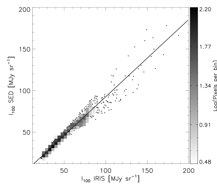
Figure 11.— Correlation between the predicted 100 µm intensity obtained by extrapolating the fitted SED and the intensity directly from the 100 µm IRIS image. The slope $0.93\pm 0.01$ of the correlation line is close to that anticipated from comparison of the power spectra. Pixels representing two-dimensional histogram is same as described in Figure 3. Individual data points are plotted where the density of points is less than or equal to three.

Second, we made a scatter plot for a pixel by pixel comparison of the brightness in each map. Figure 11 shows that the correlation is very good. For a formal linear fit we used the IDL routine SIXLIN (Isobe et al., 1990), adopting the bisector. The slope $0.93\pm 0.01$ is the same as obtained from the power spectra and the intercept $-1.5\pm 0.5$ MJy sr^-1 is close to zero as expected. The deviation of data from the correlation line at low surface brightness ($<$ 25 MJy sr^-1) is probably related to the uncertainty associated with the zero-point offsets applied to the Herschel maps (Appendix C). This comparison validates the SED parameters obtained using only Herschel data and is consistent with the expectation that most of the emission at 100 µm is due to thermal emission from big grains.

We carried out a similar exercise for 70 µm and 60 µm emission and found that the brightness was significantly underpredicted, as anticipated because of the contribution of non-equilibrium emission by smaller grains. The PACS datum plotted in Figure 1 illustrates this point.

Appendix C Assessment of Uncertainties in the SED Parameters

Errors on the parameters from the SED fit were estimated by Monte Carlo simulation (Chapin et al., 2008). For this assessment, we needed to estimate various sources of error in the intensities of the Herschel images. If these errors are realistic, then a typical SED fit would have a reduced $\chi^{2}$ close to unity and a map of $\chi^{2}$ would be featureless.

We derived the minimum absolute error for the intensities in each map from the power spectrum analysis as described in Section 2. It was clear that a constant error across the map of this order was too small in areas of high brightness; for the latter, a constant percentage error of order 5% was required to produce the expected ‘flat’ behavior in the $\chi^{2}$ map.

While investigating the details of the fits of individual SEDs for the Orion A-C1 field we found that the 350 and 500 µm data points were consistently above and below the best-fit SEDs for surface brightnesses less than 25 and 10 MJy sr^-1, respectively, and the systematic deviation increased with decreasing surface brightness. This motivated us to refine the offsets in the 350 and 500 µm maps by correlating with the 250 µm data. For the Orion A-C1 field the correlation line between 250 and 160 µm passed through the origin as expected. The correlation lines of 350 and 500 µm relative to 250 µm had intercepts of 3 and $-1.5$ MJy sr^-1, respectively. These values are of the magnitude and sign that would produce the observed systematic deviations from the best-fit SEDs for low surface brightness pixels. The two long-wavelength maps were therefore corrected by an additive offset, making the intercepts formally zero. A similar exercise on the Orion A-S1 field also led us to correct the 350, 500, and as well as 160 µm images by 2.5, 1, and $-12.0$ MJy sr^-1, respectively. These refined offsets are not perfect and we estimate an error approximately 10% of the originally applied zero-point offsets from Planck and IRAS.

Finally, we estimated the total error in the intensity to be fit by adding in quadrature the minimum absolute error, 10% of the offset value, and 5% of the intensity. These estimates ought to be conservative and do produce a flat $\chi^{2}$ image near two (as expected for four intensities, two parameters, and thus two degrees of freedom). Note that the actual values of the derived parameters are not sensitive to the precise details of the estimate of total noise.

In the Monte Carlo simulation of the uncertainties, 500 realizations of mock data were generated by adding independent Gaussian noise consistent with the above values to the actual intensities. For each realization, the SED was fit and the corresponding parameters were recorded. An uncertainty on each parameter was obtained by fitting a Gaussian to the histogram of the generated distribution. By keeping a record of each fit, we also kept track of the correlations of the uncertainties and so can produce the elliptical 1-$\sigma$ confidence intervals in, for example, the $T$ – $\tau_{1200}$ plane (see Figure 5).

References

- André et al. (2010) André, P., Men’shchikov, A., Bontemps, S., et al. 2010, A&A, 518, L102
- Arzoumanian et al. (2011) Arzoumanian, D., André, P., Didelon, P., et al. 2011, A&A, 529, L6
- Bernard et al. (2010) Bernard, J.-P., Paradis, D., Marshall, D. J., et al. 2010, A&A, 518, L88
- Boulanger et al. (1996) Boulanger, F., Abergel, A., Bernard, J.-P., et al. 1996, A&A, 312, 256
- Chapin et al. (2008) Chapin, E. L., Ade, P. A. R., Bock, J. J., et al. 2008, ApJ, 681, 428
- Chapman & Mundy (2009) Chapman, N. L., & Mundy, L. G. 2009, ApJ, 699, 1866
- Cohen et al. (2003) Cohen, M., Wheaton, W. A., & Megeath, S. T. 2003, AJ, 126, 1090
- Compiègne et al. (2011) Compiègne, M., Verstraete, L., Jones, A., et al. 2011, A&A, 525, A103
- Dobashi (2011) Dobashi, K. 2011, PASJ, 63, 1
- Fischera (2011) Fischera, J. 2011, A&A, 526, A33
- Fischera & Martin (2012a) Fischera, J., & Martin, P. G. 2012a, A&A, 547, A86
- Fischera & Martin (2012b) —. 2012b, A&A, 542, A77
- Griffin et al. (2010) Griffin, M. J., Abergel, A., Abreu, A., et al. 2010, A&A, 518, L3
- Hennemann et al. (2012) Hennemann, M., Motte, F., Schneider, N., et al. 2012, A&A, 543, L3
- Hill et al. (2011) Hill, T., Motte, F., Didelon, P., et al. 2011, A&A, 533, A94
- Isobe et al. (1990) Isobe, T., Feigelson, E. D., Akritas, M. G., & Babu, G. J. 1990, ApJ, 364, 104
- Juvela et al. (2011) Juvela, M., Ristorcelli, I., Pelkonen, V.-M., et al. 2011, A&A, 527, A111
- Kim et al. (1994) Kim, S.-H., Martin, P. G., & Hendry, P. D. 1994, ApJ, 422, 164
- Lombardi et al. (2011) Lombardi, M., Alves, J., & Lada, C. J. 2011, A&A, 535, A16
- Martin et al. (2010) Martin, P. G., Miville-Deschênes, M.-A., Roy, A., et al. 2010, A&A, 518, L105
- Martin et al. (2012) Martin, P. G., Roy, A., Bontemps, S., et al. 2012, ApJ, 751, 28
- Men’shchikov et al. (2010) Men’shchikov, A., André, P., Didelon, P., et al. 2010, A&A, 518, L103
- Miville-Deschênes & Lagache (2005) Miville-Deschênes, M.-A., & Lagache, G. 2005, ApJS, 157, 302
- Molinari et al. (2010) Molinari, S., Swinyard, B., Bally, J., et al. 2010, PASP, 122, 314
- Motte et al. (2010) Motte, F., Zavagno, A., Bontemps, S., et al. 2010, A&A, 518, L77
- Ormel et al. (2011) Ormel, C. W., Min, M., Tielens, A. G. G. M., Dominik, C., & Paszun, D. 2011, A&A, 532, A43
- Ossenkopf & Henning (1994) Ossenkopf, V., & Henning, T. 1994, A&A, 291, 943
- Peretto et al. (2012) Peretto, N., André, P., Könyves, V., et al. 2012, A&A, 541, A63
- Pilbratt et al. (2010) Pilbratt, G. L., Riedinger, J. R., Passvogel, T., et al. 2010, A&A, 518, L1
- Planck Collaboration et al. (2011a) Planck Collaboration, Abergel, A., Ade, P. A. R., et al. 2011a, A&A, 536, A24
- Planck Collaboration et al. (2011b) —. 2011b, A&A, 536, A25
- Poglitsch et al. (2010) Poglitsch, A., Waelkens, C., Geis, N., et al. 2010, A&A, 518, L2
- Preibisch et al. (1993) Preibisch, T., Ossenkopf, V., Yorke, H. W., & Henning, T. 1993, A&A, 279, 577
- Rowles & Froebrich (2009) Rowles, J., & Froebrich, D. 2009, MNRAS, 395, 1640
- Roy et al. (2010) Roy, A., Ade, P. A. R., Bock, J. J., et al. 2010, ApJ, 708, 1611
- Schneider et al. (2011) Schneider, N., Bontemps, S., Simon, R., et al. 2011, A&A, 529, A1
- Schneider et al. (2012) Schneider, N., Csengeri, T., Hennemann, M., et al. 2012, A&A, 540, L11
- Shirley et al. (2011) Shirley, Y. L., Huard, T. L., Pontoppidan, K. M., et al. 2011, ApJ, 728, 143
- Traficante et al. (2011) Traficante, A., Calzoletti, L., Veneziani, M., et al. 2011, MNRAS, 416, 2932
- Ysard et al. (2012) Ysard, N., Juvela, M., Demyk, K., et al. 2012, A&A, 542, A21