Remarks on application of different variables for the PKN model of hydrofracturing. Various fluid-flow regimes.

Abstract

The problem of hydraulic fracture for the PKN model is considered within the framework presented recently by Linkov (2011). The modified formulation is further enhanced by employing an improved regularized boundary condition near the crack tip. This increases solution accuracy especially for singular leak-off regimes. A new dependent variable having clear physical sense is introduced. A comprehensive analysis of numerical algorithms based on various dependent variables is provided. Comparison with know numerical results has been given.

Keywords: Hydraulic fracture, Numerical simulations
PACS: PACS 91.55.Fg, 91.55.Jk, 91.60.Ba
Mathematics Subject Classification(2000):MSC 74F10, 74H10, 74H15

This work has been done in the framework of the EU FP7 PEOPLE project under contract number PIAP-GA-2009-251475-HYDROFRAC.

1 Introduction

In its broadest definition, hydraulic fracturing refers to a problem of a fluid driven fracture propagating in a brittle medium. The process has been known for at least fifty years (Crittendon (1959), Desroches and Thiercelin (1993), Desroches et al. (1994), Detournay (2004), Geertsma and de Klerk (1969), Harrison et al. (1954), Hubbert and Willis (1957), Khristianovic and Zheltov (1955)). The respective technology has been utilized in the petroleum industry to intensify the extraction of hydrocarbons for decades.

Recently, due to economical reasons, it has been revived for exploiting non-conventional hydrocarbon deposits. The process has many other technological applications (e.g. disposal of waste drill cuttings underground (Moschovidis et al., 2000), geothermal reservoirs exploitation (Pine and Cundall, 1985) or $\it{in}$ $\it{situ}$ stress measurements (Desroches and Thiercelin, 1993). Hydrofracturing also appears in nature (e.g. geological processes, like magma-driven dykes (Rubin, 1995), (Lister, 1990) or a subglacial drainage of water (Tsai and Rice, 2010)). Due to the complexity of this multiphysical phenomenon, mathematical and numerical simulation of the process still represents a challenging task, in spite of the fact that immense progress has been made since the first algorithms were developed.

The mathematical model of the problem should account for coupled mechanisms driving the process, which are: i) solid mechanics equations, describing the deformation of the rock induced by the fluid pressure; ii) equations for the fluid flow within the fracture and the leak-off to the rock formation; iii) fracture mechanics criteria defining the conditions for fracture propagation. Further development of the model involves incorporation of mass transport for the proppant movement, fluid diffusion to account for the rock saturation by the leak-off flux, thermal effects affecting rheological properties of the fluid and others.

The computational challenges of the hydrofracturing models result from several factors: (i) strong non-linearity introduced by the Poiseuille equation describing the fluid flow; (ii) in the general case, a non-local relationship between the fracture opening and the net fluid pressure; (iii) moving boundaries of the fluid front and the fracture contour; (iv) degeneration of the governing PDE at the fracture front; (v) possible lag between the crack tip and the fluid front.

The first simplified mathematical descriptions of hydraulic fracture were summarized in the following three main classical models. The so-called PKN model was considered in Perkins and Kern (1961), where the authors adopted Sneddon’s solution (Sneddon and Elliot, 1946) which was further enhanced by Nordgren (1972) to account for the fluid loss effect and fracture volume change. As a result, the crack length was determined as a part of the solution. The so-called KGD (plain strain) model was developed independently by Khristianovic and Zheltov (1955), and Geertsma and de Klerk (1969). Finally, the radial or penny-shaped model was introduced by Sneddon (1946) with constant fluid pressure and was extended for the general case by Spence and Sharp (1985).

Different variations of the aforementioned models were used for treatment designs for decades, despite the fact that each of them is valid only under very specific assumptions (like elliptic cross-section of the fracture, and fracture half-length much greater than its constant height for the PKN model). Recently, the classical models have been largely replaced by the pseudo 3D models (Mack and Warpinski, 2000). A comprehensive review of the history and techniques of hydrofracturing simulation can be found in Adachi et al. (2007).

Although the classical models have been superseded in most of the practical applications, they still play a crucial role when developing and analyzing new computational algorithms. The models enable one to understand the nature of, and reasons for, computational difficulties, find the remedies for them and to extend these ideas to the general case.

Thus, in the pioneering work by Nordgren (1972), main peculiarities of the model were analyzed and a numerical algorithm was proposed to deal with the problem. Asymptotic analysis of the solution near the crack tip for impermeable rock model was presented in Kemp (1989) and an approximate solution for the zero leak-off case, with an accuracy to the first four leading asymptotic terms, was given . Here, probably for the first time, the speed equation was efficiently implemented in the model. The fourth degree of the crack opening was considered as the proper variable and used in the numerical computations. Finally, Kemp (1989) suggested to use a special tip element, compatible with the asymptotic behaviour of the solution, within the Finite Volume (FV) scheme.

For the leak-off function defined by the Carter law the two leading terms of asymptotics can be found in Kovalyshen and Detournay (2009), where the PKN problem was revisited to take into account the multi-scale arguments in the spirit of Garagash et al. (2011). The authors also used the FV scheme with a special tip element to tackle the transient regime.

Recently, the classical models of Nordgren and Spence $\&$ Sharp have been revisited again in Linkov (2011a) – Linkov (2011d). The author discovered that in some formulations the hydraulic fracture problem may exhibit ill-posed properties. To eliminate the difficulties resulting from these facts, a number of measures were proposed: i) speed equation to trace the crack front instead of the usually applied total flux balance condition; ii) the so-called $\varepsilon$-regularization technique which consists of imposing the computational domain boundary at a small distance behind the crack tip; iii) new boundary condition to be imposed in the regularized formulation; iv) new dependent variables: the particle velocity and the crack opening taken in a degree to exploit the asymptotic behaviour of the solution; v) the spatial coordinates moving with the crack front and evaluation of the temporal derivative under fixed values of these coordinates.

The advantages of the modified formulation were clearly demonstrated on the basis of developed analytical benchmarks in Linkov (2011d). An immense improvement of solution accuracy, computation efficiency and stability was shown. In Mishuris et al. (2012) a further step in employing the modified formulation was done by analyzing the stiffness of the system of differential equations arising after spatial discretization. An efficient modification of the algorithm has been proposed to trace the fracture propagation. Finally, the investigation of solution sensitivity to some process parameters has been considered.

However, the aforementioned analysis is concerned with the case when the leak-off vanishes near the crack tip and, as a result, the fluid velocity does not change much in this region.

The primary aim of this paper is to verify the recipes delivered in Linkov (2011a, b, c, d) and Mishuris et al. (2012) for an arbitrary leak off regime. In particular, the analysis includes: (i) Investigation of performance of numerical algorithms for hydrofracturing based on different formulations (different dependent and independent variables); (ii) Utilization of a new dependent variable defined as an integral of the crack opening. Such a variable has a clear physical and technological sense and is not related to any specific type of solution asymptotic behaviour near the crack tip; (iii) Modification of the way to impose boundary conditions in the framework of the $\varepsilon$-regularization technique ; (iv) Identification of optimal ranges of the various technique parameters, accuracy of computations and stiffness of the resulting dynamical systems; (v) Comparison of the solution for the Carter leak-off model with the numerical results from Kovalyshen and Detournay (2009) and discussion on the solution sensitivity.

The structure of this paper is as follows. In the next section we collect known results for the PKN model in various formulations. We restrict ourselves only to the information which is absolutely necessary to understand the paper. Subsection 2.3.2 contains an alternative formulation in terms of a new proper dependent variable - fracture volume. In Section 3 we discuss in details the numerical procedures and present main results of the computations comparing performances of different solvers under considerations. The solution obtained for the Carter leak-off model is compared with the available numerical data from Kovalyshen and Detournay (2009). The main findings of this paper are summarized in the conclusion section. Some new results concerning the asymptotic behaviour of the solutions for different leak-off regimes are presented also in Appendices A and B.

2 Problem formulation and preliminary results

2.1 Physical fundamentals and basic equations

Consider a symmetrical crack of the length $2l$ situated in the plane $x\in(-l,l)$, where the length $l=l(t)$ is one of the solution components changing as a result of the fluid flow inside the crack. The initial crack length is assumed to be nonzero: $l(0)=l_{*}>0$. There are reasonable motivations behind this assumption. Namely, for the initial (unstable) stage of the crack propagation the acceleration of the process is too large to neglect the inertial terms. For this reason, any classical model not accounting for this effect is not credible. On the other hand, in many cases the hydrofracturing process is associated with the so-called ’perforation technique’. The latter consists of the creation of a number of finger-shaped initial fractures by detonations of shaped charges spaced along the wellbore (Economides, 2000). In this way, hydrofracturing starts simultaneously from a number of non-zero length cracks. Moreover, in many rock formations (e.g. shale reservoirs) cracks already exist but are closed by the confining stress (Economides, 2000). Finally, the uncertainties involved in this complex multiphysics problem itself do not allow one to make any reliable modelling of the crack nucleation in the rock formation.

By convention, we assume that the crack is fully filled by a Newtonian liquid injected at known rate $q_{0}(t)$ at the crack mouth $x=0$.

The Poiseulle equation for the Newtonian liquid flow in a narrow channel is written in the form:

$$q=-\frac{1}{M}w^{3}\frac{\partial p}{\partial x},$$ (1)

where $q=q(t,x)$ is the fluid flow rate and $w=w(t,x)$ is the crack opening, while $p=p(t,x)$ is the net fluid pressure, that is, the difference between the fluid pressure $p_{f}$ inside the fracture and the confining stress $\sigma_{0}$ ($p=p_{f}-\sigma_{0})$. The constant $M$ involved in the equation is defined as $M=12\mu$, where $\mu$ stands for the dynamic viscosity (see for example Economides (2000)).

The continuity equation, accounting for the crack expansion and the leak-off of the fluid, may be expressed as:

$$\frac{\partial w}{\partial t}+\frac{\partial q}{\partial x}+q_{l}=0,\quad t>0,\quad 0<x<l(t),$$ (2)

where $q_{l}=q_{l}(t,x)$ is the volume rate of fluid loss to formation in the direction perpendicular to the crack surfaces per unit length of fracture.

Numerical algorithms for the PKN model, with and without leak-off, have been considered in Nordgren (1972), Kemp (1989), Kovalyshen (2010) and others. Improvements based on the speed equation and the $\varepsilon$-regularisation technique have been introduced in Linkov (2011c, d); Mishuris et al. (2012), for the case when leak-off vanishes near the crack tip. Below, we discuss the effectiveness of this approach on the three most popular leak-off models: Carter law (Carter, 1957), modified law incorporating pressure difference (Clifton and Wang, 1988) and bounded leak-off near the crack tip. An extensive discussion on possible behaviour of the leak-off function can be found in Kovalyshen (2010).

In our numerical simulations, we utilise one of the following leak-off variants:

$$q_{l}(t,x)=q_{l}^{(j)}(t,x)+q_{j}^{*}(t,x),\quad j=1,2,3,$$ (3)

where

$$\begin{array}[]{l}\displaystyle q_{l}^{(1)}=\frac{C_{1}(t)}{\sqrt{t-\tau(x)}},\quad q_{l}^{(2)}=\frac{C_{2}(t)p}{\sqrt{t-\tau(x)}},\quad\displaystyle q_{l}^{(3)}=C_{31}(t)p+C_{32}(t),\quad\quad 0<x<l(t).\end{array}$$ (4)

Here $C_{1}=C_{L}$ is usually assumed to be a known constant defined experimentally (Carter, 1957). Recently it was estimated analytically for a poro-elastic material in Kovalyshen (2010). The function $\tau(x)$ contains information on the history of the process. It defines the time at which the fracture tip reaches the point $x$ and can be computed as the inverse of the crack length:

$$\tau(x)=l^{-1}(x),\quad x>l_{*}.$$ (5)

For $x\leq l_{*}$ we conventionally set $\tau(x)\equiv 0$. Other constants in (4), $C_{j}(t)=C_{j}(t,w,p)$, ($j=2,3$) may depend on the solution itself but are bounded functions in time. Finally, we assume that the terms $q_{j}^{*}$, ($j=1,2,3$) in (4) are negligible in comparison with $q_{l}^{(j)}$ near the crack tip. Note that application of the Carter leak-off law (Carter, 1957) which is a simplified model of established fluid diffusion through the fracture walls, may be not justified at some stages of the process (Nordgren, 1972; Lenoach, 1995; Mathias et al., 2009).

In this paper, we are aiming to build a general numerical framework for the problem under consideration. Thus, the collection of possible leak-off representations given in (4) covers the whole spectrum of possible bahaviours used in the hydrofracturing simulations (Kovalyshen, 2010).

The system of equations (1) - (2) should be supplemented by the elasticity equation. We consider the simplest relationship used in the PKN formulation

$$p=kw,$$ (6)

with a known proportionality coefficient $k=\frac{2}{\pi h}\frac{E}{1-\nu^{2}}$ found from the solution of a plane strain elasticity problem for an elliptical crack of height $h$ (Nordgren, 1972). Constants $E$ and $\nu$ are the Young modulus and the Poisson ratio, respectively. In physical interpretation, this condition refers to the case when the fracture resistance of the solid is so small, that the energy dissipated by the fracture extension is negligible compared to the energy dissipated in the viscous fluid flow (Adachi and Detournay, 2002). However, it turns out that, even in the models where the toughness dominated regime can be accounted for, it may be of a minor importance. For example, in Savitski and Detournay (2002) it has been proven that radial hydraulic fractures in impermeable rocks generally propagate in the viscosity regime, and that the toughness regime is relevant only in exceptional circumstances (for the average values of the field parameters the fracture would remain in the viscosity dominated regime for many years).

On substitution of the Poiseulle equation (1) and elasticity relationship (6) into the continuity equation (2), one obtains a well known lubrication (Reynolds) equation defined in the trapezoidal domain ($t>0,\,\,0<x<l(t)$):

$$\frac{\partial w}{\partial t}-\frac{k}{M}\frac{\partial}{\partial x}\left(w^{3}\frac{\partial w}{\partial x}\right)+q_{l}=0.$$ (7)

Since the system has its natural symmetry with respect to variable $x$ and the equations are local, it is convenient to consider only half (symmetrical part) of the interval $[0,l(t)]$ instead of the full crack length $[-l(t),l(t)]$.

Following the discussion on the initial crack length above, the initial conditions for the problem are:

$$l(0)=l_{*},\quad w(0,x)=w_{*}(x),\quad x\in(0,l_{*}).$$ (8)

The boundary conditions include: known fluid injection rate at the crack mouth, $q_{0}$, zero crack opening and zero fluid flux rate at the crack tip:

$$q(t,0)=q_{0}(t),\quad w(t,l(t))=0,\quad q(t,l(t))=0.$$ (9)

Note that the problem formulated in this way looks overdetermined as the governing equation (7) is of the second order with respect to spatial variable. This issue shall be discussed later.

Finally, by consecutive integration of equation (7) over time and then space, one can also derive the standard formula for the global fluid balance in the form:

$$\begin{array}[]{l}\displaystyle\int_{0}^{l(t)}[w(t,x)-w_{*}(x)]dx-\int_{0}^{t}q_{0}(t)dt+\int_{0}^{l(t)}\int_{0}^{t}q_{l}(t,x)dtdx=0,\end{array}$$ (10)

where it is accepted that $w_{*}(x)=0$ when $x>l_{*}$ and $l^{\prime}(t)\geq 0$.

As has been shown in Linkov (2011d), the crucial role in the analysis of the problem plays the particle velocity defined in the following manner:

$$V(t,x)=\frac{q}{w},\quad t>0,\quad 0\leq x\leq l(t),$$ (11)

which indicates the average velocity of fluid flow through the cross-sections of the fracture.

Under the assumption that the crack is fully filled by the fluid and sucking, ejection or discharge through the front can be neglected, the fluid velocity defines the crack propagation speed and the following speed equation is valid (Kemp, 1989; Linkov, 2011a, b):

$$l^{\prime}(t)=V\left(t,l(t)\right),\quad t>0.$$ (12)

Moreover, for physical reasons, one can assume that the fluid velocity at the crack tip is finite

$$0\leq V\left(t,x\right)<\infty,\quad t>0,\quad x\leq l(t)$$ (13)

Note that, allowing the crack propagation speed to be infinite, one has to simultaneously include the inertia term in the equations. Thus, the estimate (13) is a direct consequence of neglecting the acceleration terms.

2.2 Asymptotic behaviour of the solution and its consequences

As was mentioned in Spence and Sharp (1985), the fact that both $w$ and $q$ are present in (11), creates serious difficulties when trying to use the fluid velocity as a variable. However, as shown in Linkov (2011a, b, c, d), proper usage of fluid velocity may be extremely beneficial. First, it allows one to replace two boundary conditions at the crack tip (9)_2,3 with a single one additionally incorporating information from the speed equation (12), (13).

Indeed, the boundary conditions (9)_2,3 in view of (1) and (6) lead to the estimate

$$w(t,x)=o\left((l(t)-x)^{\frac{1}{4}}\right),\quad x\rightarrow l(t),$$ (14)

which does not necessarily guarantee (13). However, further analysis of the problem, for different leak-off functions (see Kemp (1989); Kovalyshen and Detournay (2009) and Appendix B of this paper), shows that the particle velocity is bounded near the crack tip and the crack opening exhibits the following asymptotic behaviour:

$$\begin{array}[]{l}w(t,x)=w_{0}(t)\big{(}l(t)-x\big{)}^{\frac{1}{3}}+w_{1}(t)\big{(}l(t)-x\big{)}^{\alpha}+\,o\big{(}(l(t)-x)^{\alpha}\big{)},\quad\text{as}\quad x\rightarrow l(t),\end{array}$$ (15)

with some $\alpha>1/3$. For the classical PKN model for an impermeable solid (or when leak-off vanishes near the crack tip at least as fast as the crack opening) the exponent $\alpha=4/3$ was found in Kemp (1989). For the case of the singular Carter’s type leak-off, the exponent $\alpha=1/2$ was determined in Kovalyshen and Detournay (2009).

Note that the asymptotics (15) shows that fluid velocity is indeed bounded near the crack tip. Moreover,

$$V(t,x)=V_{0}(t)+V_{1}(t)\big{(}l(t)-x\big{)}^{\beta}+o\big{(}(l(t)-x)^{\beta}\big{)},$$ (16)

as $x\to l(t)$, where $\beta=\alpha-1/3$ and

$$V_{0}=\frac{k}{3M}w_{0}^{3}(t),\quad V_{1}=\frac{k}{M}\left(\alpha+\frac{2}{3}\right)w_{0}^{2}(t)w_{1}(t).$$ (17)

As follows from Appendix B, $V(t,x)$ may not be so smooth near the crack tip as one could expect and the exponent $\beta$ in (16) plays an important role for this. Indeed, if $\beta\geq 1$ then $V(t,\cdot)\in C^{1}[0,l(t)]$ and the particle velocity function is smooth enough near the crack tip. However, this happens only in the special case of $\alpha=4/3$ when $V_{x}(t,x)$ is bounded near the crack tip. In case of singular leak-off ($0<\beta<1$), the particle velocity near the crack tip is only of the Hölder type $V(t,\cdot)\in C^{1}[0,l(t))\bigcap H^{\beta}[0,l(t)]$. In Appendix B we present an exact form of the asymptotic expansion (15), which yields the aforementioned smoothness deterioration of $V$ near the crack tip for the singular leak-off models.

Note that estimate (15) (or (16)) is equivalent to the condition (13). Thus, in view of (11), the pair of conditions (9)₂ and (9)₃ is equivalent to (9)₂ and (15). This discussion clearly illustrates why accounting for asymptotic behaviour of the solution in form (15) is of crucial importance for effective numerical realisation of any algorithm utilised in hydrofracturing (Adachi and Peirce, 2007; Garagash et al., 2011; Mitchell et al., 2007). On the other hand, the fact that the particle velocity function is smooth enough near the crack tip has been one of the important arguments to use the speed equation and proper variable approach as the basis for improvement of the existing numerical algorithms (Linkov, 2011a). It should be emphasized that behaviour of $V(t,x)$ near the crack tip may have serious implications when using $\varepsilon$-regularization technique.

Therefore, the main aim of this paper is to show that, regardless of possible smoothness of the particle velocity near the crack tip, the approach proposed in Linkov (2011a) – Linkov (2011d) and Mishuris et al. (2012) is still efficient.

2.3 Normalised formulation

Let us normalize the problem by introducing the following dimensionless variables:

$$\tilde{x}=\frac{x}{l(t)},\quad\tilde{t}=\frac{t}{t_{n}},\quad t_{n}=\frac{M}{kl_{*}},\quad\tilde{w}_{*}(\tilde{x})=w_{*}(x),$$

$$\tilde{w}(\tilde{t},\tilde{x})=\frac{w(t,x)}{l_{*}},\quad\tilde{V}(\tilde{t},\tilde{x})=\frac{t_{n}}{l_{*}}V(t,x),\quad L(\tilde{t})=\frac{l(t)}{l_{*}},$$

$$l^{2}_{*}\tilde{q}_{0}(\tilde{t})=t_{n}q_{0}(t),\quad l_{*}\tilde{q}_{l}(\tilde{t},\tilde{x})=t_{n}q_{l}(t,x),$$ (18)

where $\tilde{x}\in(0,1)$ and $L(0)=1$.

Using this notation, one defines the normalised particle velocity as:

$$\tilde{V}(\tilde{t},\tilde{x})=-\frac{\tilde{w}^{2}}{L(\tilde{t})}\frac{\partial\tilde{w}}{\partial\tilde{x}}.$$ (19)

The conservation law (2) in the normalised domain is rewritten in the following manner:

$$\frac{\partial\tilde{w}}{\partial\tilde{t}}=\frac{1}{L(\tilde{t})}\left[\left(\tilde{x}\tilde{V}(\tilde{t},1)-\tilde{V}(\tilde{t},\tilde{x})\right)\frac{\partial\tilde{w}}{\partial\tilde{x}}-\tilde{w}\frac{\partial\tilde{V}}{\partial\tilde{x}}\right]-\tilde{q}_{l}(\tilde{t},\tilde{x}),$$ (20)

The leading terms of the asymptotic estimate of the leak-off function from (4) are now:

$$\tilde{q}_{l}^{(1)}(\tilde{t},\tilde{x})=\frac{\tilde{C}_{1}(\tilde{t})D\left(\tilde{t}\right)}{\sqrt{1-\tilde{x}}},\,\,\,\tilde{q}_{l}^{(2)}(\tilde{t},\tilde{x})=\frac{\tilde{C}_{2}(\tilde{t})D\left(\tilde{t}\right)}{\sqrt{1-\tilde{x}}}\tilde{w}(\tilde{t},\tilde{x}),\quad\tilde{q}_{l}^{(3)}(\tilde{t},\tilde{x})=\tilde{C}_{31}(\tilde{t})\tilde{w}(\tilde{t},\tilde{x})+\tilde{C}_{32}(\tilde{t}).$$ (21)

Here, the function

$$D\left(\tilde{t}\right)=\sqrt{\frac{L^{\prime}\left(\tilde{t}\right)}{L\left(\tilde{t}\right)}},$$ (22)

is introduced in the Appendix A, where the remainder between the normalised total flux and the leading term (21) has been effectively estimated. Thus the normalised term $\tilde{q}^{*}_{j}(\tilde{t},\tilde{x})$ vanishes near the crack tip faster than the solution itself.

Finally, normalised initial conditions (8) and boundary conditions (9) are:

$$L(0)=1,\quad\tilde{w}(0,\tilde{x})=\tilde{w}_{*}(\tilde{x}),\quad x\in(0,1),$$ (23)

and

$$-\frac{1}{L(\tilde{t})}\tilde{w}^{3}\frac{\partial\tilde{w}}{\partial\tilde{x}}(\tilde{t},0)=\tilde{q}_{0}(\tilde{t}),\quad\tilde{w}(\tilde{t},1)=0.$$ (24)

The global fluid balance (10) can be written in the form:

$$L(\tilde{t})\int_{0}^{1}\tilde{w}(\tilde{t},x)dx-\int_{0}^{1}\tilde{w}(x,0)dx-\int_{0}^{\tilde{t}}\tilde{q}_{0}(t)dt+\int_{0}^{\tilde{t}}L(t)\int_{0}^{1}\tilde{q}_{l}(t,x)dxdt=0.$$ (25)

For convenience, from this point on we will omit the ”$\sim$” symbol for all dependent and independent variables and will only consider the respective dimensionless values.

Note that the particular representation (20) of the Reynolds equation highlights an essential feature of the problem - it is singularly perturbed near the crack tip. Indeed, both coefficients in front of the spatial derivatives on the right-hand side of the equation (20) tend to zero at $x=1$. Thus, the asymptotic behaviour of the solution near the crack tip ($x\to 1$)

$$w=w_{0}(t)\left(1-x\right)^{\frac{1}{3}}+w_{1}(t)\left(1-x\right)^{\alpha}+o\left((1-x)^{\alpha}\right),$$ (26)

$$V=V_{0}(t)+V_{1}(t)\left(1-x\right)^{\alpha-\frac{1}{3}}+o\left((1-x)^{\alpha-\frac{1}{3}}\right),$$ (27)

represents nothing but the boundary layer. Moreover, normalizing (17)₁ one obtains:

$$V_{0}(t)=\frac{1}{3L(t)}w_{0}^{3}(t).$$ (28)

The terms $w_{0}$, $w_{1}$ and $V_{0}$, $V_{1}$ in (26) and (27) are different from those in (15) and (16). In fact, the former should be written with ”$\sim$” symbol.

On substitution of (19) into (20), one eliminates the particle velocity function from Reynolds equation:

$$\frac{\partial w}{\partial t}=\frac{1}{L^{2}(t)}\left[\frac{1}{3}w_{0}^{3}x\frac{\partial w}{\partial x}+3\tilde{w}^{2}\left(\frac{\partial w}{\partial x}\right)^{2}+w^{3}\frac{\partial^{2}w}{\partial x^{2}}\right]-q_{l}.$$ (29)

Here $w_{0}$ is the multiplier of the first term of the asymptotic expansion (15). This form of lubrication equation exhibits the same degenerative properties as (20). Also the coefficients appearing in front of the leading terms tend to zero near the crack tip.

The speed equation (12) defining the crack propagation speed is given in the normalised variables as:

$$L^{\prime}(t)=V_{0}(t),\quad t>0.$$ (30)

Taking into account (28), the latter can be rewritten in the following form

$$\frac{d}{dt}L^{2}=\frac{2}{3}w_{0}^{3}(t),\quad\quad t>0.$$ (31)

This equation serves us to determine the unknown value of the crack length $L(t)$. As it has been shown in Mishuris et al. (2012), such an approach has clear advantages over the standard one based on the global fluid balance equation (25).

As a result of the foregoing transformations, one can formulate a system of PDEs describing the hydrofracturing process. The system is composed of two operators:

$$\frac{d}{dt}w=\mathcal{A}_{w}(w,L^{2}),\quad\frac{d}{dt}L^{2}(t)=\mathcal{B}_{w}(w),$$ (32)

where $\mathcal{A}_{w}$ is defined by the right-hand side of equation (29) with the boundary conditions (24)_1,2, while the second operator $\mathcal{B}_{w}$ is given by (31). The system is equipped with the initial conditions:

$$L(0)=1,\quad w(0,x)=w_{*}(x),\quad x\in(0,1).$$ (33)

2.3.1 Reformulation of the problem in proper dependent variables. First approach

In Linkov (2011d) and later in Mishuris et al. (2012) it has been shown that the dependent variable

$$U(t,x)=w^{3}(t,x)$$ (34)

is more favorable for the solution of the system (32), (33) than the crack opening itself. This idea is based on the fact that, according to the asymptotics of the solution near the crack tip, the dependent variable $U$ is much smoother than $w$. In the case of an impermeable solid, the solution $U$ is analytic in the closed interval $[0,1]$ (see Linkov (2011d)). However, the type of leak-off function is of significant importance here. Thus, adopting asymptotic representation (26), one can see that for $x\to 1$

$$U=U_{0}(t)(1-x)+U_{1}(t)(1-x)^{\frac{2}{3}+\alpha}+o((1-x)^{\frac{1}{3}+2\alpha}),$$ (35)

where the coefficients $U_{0}(t)$ and $U_{1}(t)$ are directly related to those appearing in the crack opening formulation:

$$U_{0}(t)=w_{0}^{3}(t),\quad U_{1}(t)=w_{0}^{2}(t)w_{1}(t).$$ (36)

Depending on the type of leak-off described in (4), the exponent in the second asymptotic term $\frac{2}{3}+\alpha$ may take value $3/2$, $11/6$ or 2, respectively. Thus in the first two cases, the transformation (34) no longer results in polynomial representations of asymptotic expansion for $U$. For this reason, the advantage of the approach using variable $U$ in more general cases, when the leak-off is singular near the crack tip, should still be confirmed. This is one of the aims of this paper. On the other hand, at least two factors work in favor of this formulation. First, the spatial derivative of $U$ is not singular and, second, the particle velocity is given by a linear relationship

$$V(t,x)=-\frac{1}{3L(t)}\frac{\partial U}{\partial x}.$$ (37)

The governing equation (20) in terms of the new variable can be written in the normalized domain $x\in(0,1)$ as:

$$\frac{\partial U}{\partial t}=\frac{1}{L(t)}\left[\left(xV(t,1)-V(t,x)\right)\frac{\partial U}{\partial x}-3U\frac{\partial V}{\partial x}\right]-3U^{\frac{2}{3}}q_{l},$$ (38)

Similarly to (29) the particle velocity function may be eliminated from the lubrication equation:

$$\frac{\partial U}{\partial t}=\frac{1}{3L^{2}(t)}\left[xU_{0}\frac{\partial U}{\partial x}+\left(\frac{\partial U}{\partial x}\right)^{2}+3U\frac{\partial^{2}U}{\partial x^{2}}\right]-3U^{\frac{2}{3}}q_{l}.$$ (39)

Note that equations (38)-(39) are of a very similar structure to those evaluated for the crack opening $w$. They exhibit the same degenerative nature near the crack tip.

Finally, boundary conditions (24) transform to:

$$-\frac{\sqrt[3]{U(t,0)}}{3L(t)}\frac{\partial}{\partial x}U(t,0)=q_{0}(t),\quad U(t,1)=0,$$ (40)

while the speed equation (31) takes the following form:

$$\frac{d}{dt}L^{2}=\frac{2}{3}U_{0}(t),\quad\quad t>0.$$ (41)

The system of PDEs equivalent to (32) is now defined as:

$$\frac{d}{dt}U=\mathcal{A}_{U}(U,L^{2}),\quad\frac{d}{dt}L^{2}(t)=\mathcal{B}_{U}(U).$$ (42)

The operator $\mathcal{A}_{U}$ is described by (39) with boundary conditions (40), while the second operator $\mathcal{B}_{U}$ is given by (41). Finally, the initial conditions are similar to those in the previous formulation (23):

$$L(0)=1,\quad U(0,x)=w_{*}^{3}(x),\quad x\in(0,1).$$ (43)

2.3.2 Reformulation of the problem in proper dependent variables. Second approach

The aforementioned formulation of the problem in terms of the dependent variable $U$ has one considerable drawback. It is well known that for different elasticity models and different hydrofracturing regimes one has various asymptotic behaviours of the solution near the crack tip (Adachi and Detournay, 2002). For example, for exact equations of elasticity theory and the zero toughness condition ($K_{IC}=0$), the exponent of the leading term of $w$ varies from 2/3, for the Newtonian fluid, to 1, for the ideally plastic fluid. Thus, the same reformulation to the type of the proper variable might be inconvenient, or even impossible.

For this reason, we introduce another dependent variable. Although it does not transform the asymptotic behaviour of the solution in such a smooth manner as it has been done previously when adopting $U$, this variable has its own advantages. Namely, let us consider a new dependent variable $\Omega$ defined as follows:

$$\Omega(t,x)=\int_{x}^{1}w(t,\xi)d\xi.$$ (44)

This variable is not directly related to any particular asymptotic representation of $w(x,t)$, however it assumes that $w\to 0$ for $x\to 1$. As a result the form of governing equations for $\Omega$ remains the same regardless of $w(x,t)$ asymptotics, i.e. this formulation has a general (universal) character. Note, that in case of $U$ the optimal way of transformation for the lubrication equation essentially depends on the exact form of asymptotic expansion (the leading term) for $w$.
Another advantage of $\Omega$ comes from the fact that it has clear physical and technological interpretation. Namely, it reflects the crack volume measured from the crack tip.

Asymptotics of the function $\Omega$ near the crack tip takes the following form:

$$\begin{split}\Omega(t,x)=\Omega_{0}(t)(1-x)^{\frac{4}{3}}+\Omega_{1}(t)(1-x)^{\alpha+1}+o((1-x)^{\alpha+1}),\quad x\rightarrow 1,\end{split}$$ (45)

where the coefficients $\Omega_{0}(t)$ and $\Omega_{1}(t)$ are related to those in (26):

$$\Omega_{0}(t)=\frac{3}{4}w_{0}(t),\quad\Omega_{1}(t)=\frac{1}{\alpha+1}w_{1}(t).$$ (46)

Thus, similarly to $U$, the new variable is smoother than the crack opening, $w$, and the first singular derivative of $\Omega$ is that of the second order.

By spatial integration of (20) from $x$ to 1 and substitution of (44) one obtains:

$$\frac{\partial\Omega}{\partial t}=-\frac{1}{L(t)}\left[\big{(}V(t,x)-xV(t,1)\big{)}\frac{\partial\Omega}{\partial x}+V(t,1)\Omega\right]-Q_{l},$$ (47)

where the monotonicity of $L^{\prime}(t)>0$ has been taken into account and

$$Q_{l}(t,x)=\int_{x}^{1}q_{l}(t,\xi)d\xi.$$

Here, the particle velocity (19) is computed in the manner:

$$V(t,x)=\frac{1}{3L(t)}\frac{\partial}{\partial x}\left(\frac{\partial\Omega}{\partial x}\right)^{3}\!\!\!.$$ (48)

By eliminating $V(x,t)$ from the equation (47) we derive a new formula for the lubrication equation:

$$\frac{\partial\Omega}{\partial t}=-\frac{1}{L^{2}(t)}\left[\left(\frac{\partial\Omega}{\partial x}\right)^{\!3}\frac{\partial^{2}\Omega}{\partial x^{2}}+\frac{64}{81}\Omega_{0}^{3}\left(\Omega-x\frac{\partial\Omega}{\partial x}\right)\right]-Q_{l}.$$ (49)

The boundary conditions (24) are expressed in the following way:

$$-\frac{1}{L(t)}\left(\frac{\partial\Omega}{\partial x}\right)^{3}\frac{\partial^{2}\Omega}{\partial x^{2}}(t,0)=q_{0},\quad\frac{\partial\Omega}{\partial x}(t,1)=0.$$ (50)

Interestingly, the first boundary condition, directly substituted into the lubrication equation (47) can be equivalently rewritten in the form

$$\frac{\partial\Omega}{\partial t}(t,0)=-\frac{64}{81^{2}L(t)}\Omega(t,0)\Omega_{0}^{3}(t)+\frac{q_{0}(t)}{L(t)}-Q_{l}(t,0),$$ (51)

This condition, in turn, represents nothing but the local (in time) flux balance condition. To verify this, it is enough to apply the time derivative to the equation (25). Furthermore it appears much easier for implementation into a numerical procedure than (50)₁ itself, but may lead to some increase of the problem stiffness, as we will show later.

It is easy to check, by using the governing equation (47) and limiting values of all its terms for $x\to 1$ , that a weaker boundary condition

$$\Omega(t,1)=0$$ (52)

is equivalent to the original one (50)₂. Finally, the speed equation (31) in the $\Omega$ formulation assumes the following form:

$$\frac{d}{dt}L^{2}(t)=\frac{128}{81}\Omega_{0}^{3}(t).$$ (53)

In this way we obtain another system of PDEs that is composed of two operator relations:

$$\frac{d}{dt}\Omega=\mathcal{A}_{\Omega}(\Omega,L^{2}),\quad\frac{d}{dt}L^{2}(t)=\mathcal{B}_{\Omega}(\Omega),$$ (54)

where, as previously, $\mathcal{A}_{\Omega}$ is defined by (29) with boundary conditions (50)_1,2 or (51) and (52). The second operator, $\mathcal{B}_{\Omega}$, is given by equation (53). Here the initial conditions are obtained from (23):

$$L(0)=1,\quad\Omega(0,x)=\Omega_{*}(x)\equiv\int_{x}^{1}w_{*}(\xi)d\xi.$$ (55)

2.4 $\varepsilon$-regularization and the respective boundary conditions

In our analysis we are going to use the so-called $\varepsilon$-regularization technique. It was originally introduced in Linkov (2011a) for the system of spatial coordinates moving with the fracture front. In Mishuris et al. (2012), the authors efficiently adopted the approach for the normalised coordinate system.

The reason to separate the domain from the end point $x=1$ by a small distance of $\varepsilon$ and to introduce $\varepsilon$-regularisation has been thoroughly described in Linkov (2011a). It consists of replacing the Dirichlet boundary condition (40)₂ with an approximate one:

$$U(t,1-\varepsilon)=3\varepsilon L(t)V(t,1),$$ (56)

emerging from deep physical arguments. The value of the crack propagation speed $V(t,1)$ (and simultaneously the particle velocity at a fracture tip) was suggested to be computed from the speed equation (41) in its approximated form:

$$V(t,1)=-\frac{1}{3L(t)}\frac{\partial U}{\partial x}(t,1-\varepsilon).$$ (57)

The pair of conditions (56) – (57) has shown an excellent performance in terms of solution accuracy and, as has been proven in Mishuris et al. (2012), reduced the stiffness of dynamic system in case of leak-off function vanishing near the crack tip. One can check that for such a leak-off model numerical error introduced by using the approximate conditions, instead of the exact ones, is of the order $O(\varepsilon^{2})$. In view of all improvements following from utilisation of the regularized conditions (Linkov (2011d); Mishuris et al. (2012)) such a strategy is fully justified and in fact inevitable.

The conditions can be written in an equivalent form. Indeed, one can merge (56) and (57) into a single condition of the third type:

$$U(t,1-\varepsilon)+\varepsilon\frac{\partial U}{\partial x}(t,1-\varepsilon)=0.$$ (58)

Interestingly, the latter condition is nothing but the consequence of a direct utilization of the information about the leading term of asymptotics of the solution near the crack tip (compare with (35)).

Analogously, one can define the respective pairs of boundary conditions in the regularized formulations. Considering the dependent variable $w$ one should take (31) together with the condition

$$w(t,1-\varepsilon)+3\varepsilon\frac{\partial w}{\partial x}(t,1-\varepsilon)=0,$$ (59)

while analysing the system based on the dependent variable $\Omega$, the speed equation (53) should be accompanied by

$$4\Omega(t,1-\varepsilon)+3\varepsilon\frac{\partial\Omega}{\partial x}(t,1-\varepsilon)=0.$$ (60)

To conclude this subsection, one can make a prediction that in the case of a singular leak-off function, even when using the $\varepsilon$-regularization technique, the accuracy of the solution should be worse than that presented in Linkov (2011a),Mishuris et al. (2012). However, it is always possible to use information on accurate asymptotic behaviour of the solution (employing higher order terms) and in this way improve the accuracy of computations.

3 Numerical solution of the dynamic systems

In this section, three alternative systems of PDEs (32), (42) and (54) describing the problem of hydrofracruing are transformed into the corresponding non-linear dynamic systems of the first order. Then, on the basis of respective analytical benchmarks, we analyze their stiffness properties, the accuracy and efficiency of computations. The benchmark solutions in question are described in Appendix C.

3.1 Representation of the boundary conditions and the speed equation

Consider a spatial domain of the problem reduced in accordance with the $\varepsilon$-regularization technique to the interval $x\in[0,1-\varepsilon]$, where $\varepsilon$ is a small parameter. Let the mesh, $\{x_{j}\}_{j=1}^{N}$, be composed of $N$ nodes with $x_{1}=0$ and $x_{N}=1-\varepsilon$.

For each of the problem formulations, two boundary conditions should be accounted for: one specified at the crack inlet and a regularized boundary condition at $x=1-\varepsilon$. In the following we present a brief description of how these conditions are introduced to the numerical scheme.

From now on, for the dependent variables discussed above ($w(t,x)$, $U(t,x)$, $\Omega(t,x)$), we use common notation $f(t,x)$ together with a convention $f_{k}=f(t,x_{k})$.

To discretize the first boundary condition (depending on the formulation: (24)₁, (40)₁ or (50)₁) we exploit the smooth character of the solution near the point $x=0$. Thus, accepting a polynomial approximation of $f(x,t)$ on the interval $x\in[x_{1},x_{3}]$, the respective nonlinear relation between $f_{1}$, $f_{2}$ and $f_{3}$ may be derived:

$$A_{1}(f_{1},t)f_{1}+A_{2}(f_{1},t)f_{2}+A_{3}(f_{1},t)f_{3}=q_{0}.$$ (61)

As mentioned in 2.4, the regularized boundary condition in the $\varepsilon$-regularization technique proposed in Linkov (2011a) is equivalent to a mixed boundary condition based on the leading term of the asymptotic expansion (see (58), (59), (60)). Below we propose a modification of this approach which consists in employing two terms of the asymptotics. We will show that such a strategy prevents the deterioration of accuracy when the solution is not so smooth as in the cases originally considered in Linkov (2011a), Mishuris et al. (2012).

According to (26), (35) and (45), the following asymptotics approximation is acceptable in the proximity of the crack tip ($x\in[x_{N-2},1]$):

$$f(t,x)=e_{1}^{(f)}(t)(1-x)^{\alpha_{1}}+e_{2}^{(f)}(t)(1-x)^{\alpha_{2}}.$$ (62)

The values of $\alpha_{1}$ and $\alpha_{2}$ are known in advance and depend, as has been discussed above, on the chosen variable and the behavior of the leak-off function. Assuming that the last three points of the discrete solution $(x_{N-2},f_{N-2})$, $(x_{N-1},f_{N-1})$ and $(x_{N},f_{N})$ lie on the solution graph $(x,f(t,x))$, one can derive a formula combining all these values in one equation:

$$f_{N}+b_{N-1}^{(f)}f_{N-1}+b_{N-2}^{(f)}f_{N-2}=0,$$ (63)

where $b_{j}^{(f)}=b_{j}^{(f)}(x_{N-2},x_{N-1},x_{N})$. Relation (63) is consequently used to represent the regularised boundary condition at $x=1-\varepsilon$.

Remark 1. In the authors opinion, the presented approach is a direct generalization of that proposed in Linkov (2011a). Indeed, if one takes $e_{2}=0$ in the representation (62) then the pair of the equations (58) and (57) follows immediately. If $\alpha_{2}^{(f)}-\alpha_{1}^{(f)}=1$, which means that the leak-off function $q_{l}$ is bounded near the crack tip, the second asymptotic term provides a small correction. However, in the case of the Carter law, when $\alpha_{2}^{(f)}-\alpha_{1}^{(f)}=1/6$, it brings an important contribution and improves the accuracy of the computations, as will be shown later.

Finally, coefficient $e_{1}$ from (62) is substituted into the pertinent form of the speed equation (31), (41) or (53) to give the ordinary differential equations for the crack length:

$$\frac{d}{dt}L^{2}=\frac{2}{3}\left(e_{1}^{(w)}\right)^{3},\quad\frac{d}{dt}L^{2}=\frac{2}{3}e_{1}^{(U)},\quad\frac{d}{dt}L^{2}(t)=\frac{128}{81}\left(e_{1}^{(\Omega)}\right)^{3}.$$ (64)

Note that the right-hand sides of the equations define the boundary operators $\mathcal{B}_{w}$, $\mathcal{B}_{U}$ and $\mathcal{B}_{\Omega}$ from (32)₂, (42)₂ or (54)₂, respectively.

Remark 2. As it follows from this analysis, the $\varepsilon$-regularization is, in a sense, equivalent to the introduction of a special tip element in the discrete solution. Thus, one can see a complementarity with the approach utilised in Kovalyshen (2010). However, and this is crucial for the analysis, only the speed equation together with $\varepsilon$-regularization allows to take into account both the local and global phenomena, and to do this in the most efficient way from the numerical point of view.

Remark 3. In the case of the dependent variable $U$, apart from the representations (62) of the boundary condition near the crack tip in the linear form

$$U_{N}=b_{1}^{(U)}U_{N-1}+b_{2}^{(U)}U_{N-2},$$ (65)

one can use a nonlinear one, adopting the relationship between this dependent variable and the crack opening $w$:

$$U_{N}=\left(b_{1}^{(w)}\sqrt[3]{U_{N-1}}+b_{2}^{(w)}\sqrt[3]{U_{N-2}}\right)^{3}.$$ (66)

Note that the two terms representation (65) of the function $U$ is less informative than the same representation for the functions $w$ (or $\Omega$) and thus, using the modified condition (66), one can expect a better solver performance.

3.2 Spatial discretization of the Reynolds equation. Corresponding dynamic systems

Let us consider the Reynolds equations written in different dependent variables ((32), (42) or (54), respectively). By representing the spatial derivatives in the right-hand sides of the corresponding equation by central three point finite difference schemes, we obtain a nonlinear system of $N-2$ ordinary differential equations for the values $f_{i}(t)$ at each internal point of the spatial domain ($x_{2},...,x_{N-1}$). The respective boundary conditions are embedded into the system through equations (61) and (63).

Supplementing the system with the pertinent form of the speed equation (64), we obtain a non-linear dynamic system of first order describing the process of hydrofracturing which can be written in the form:

$${\bf F}^{\prime}={\bf A}^{(f)}{\bf F}+{\bf G}^{(f)},$$ (67)

where ${\bf F}={\bf F}(t)$ is a vector of unknown solution $[f(t,x_{1}),$ $f(t,x_{2}),\ldots,f(t,x_{N}),L^{2}(t)]$ of dimension $N-1$. Note that matrix ${\bf A}^{(f)}$ and vector ${\bf G}^{(f)}$ depend, generally speaking, on the solution. Matrix $\bf A$ is the so-called mass matrix of the system, in the case of which a tri-diagonal form prevails (however the boundary conditions and the last equation for $L^{2}(t)$ disturb the tri-diagonal structure).

Remark 4 In the case when the boundary condition in formulation (51) is in use, the dimension of the dynamic system is $N$. Indeed, this condition has the form of an ODE, and thus can be substituted directly into the system as an additional equation.

In our numerical computations two different types of spatial meshes are used. The first one is a regular mesh with uniformly spaced nodes, while the second one gives an increased nodes density when approaching the crack tip. Both types of meshes can be described by the formula:

$$x_{m}(\delta)=1-\left(1-\left(1-\varepsilon^{\frac{1}{\delta}}\right)\frac{m}{N}\right)^{\delta},\quad m=1,...,N.$$ (68)

In the foregoing, the parameter $\delta$ defines the mesh type. Namely, for $\delta=1$ one has the uniform mesh (henceforth denoted as $x^{(I)}$), since any $\delta>1$ gives the nodes concentration near the crack tip (this mesh will be referred to as $x^{(II)}(\delta)$). Mesh $x^{(II)}(\delta)$ allows one to choose appropriate parameter $\delta$ to suppress the stiffness of dynamic system or to increase the solution accuracy.

The stiffness of a dynamic system may be described by the condition number or the condition ratio (Aiken, 1985) of a mass matrix ${\bf A}^{(f)}$. In general, the values given by various measures are different (see some consequences in Mishuris et al. (2012)). In this paper we use the condition ratio as the measure of the system stiffness. Some rough estimation of this parameter may help to choose an optimal value of $\delta$ from the stiffness point of view. In the case under consideration, one can analyse the condition ratio of a simplified variant of the system (39), where only the leading term (with the second order derivative) is preserved and the nonlinear multiplier is substituted by the first term of the asymptotic expansion for $U$. It turns out that $\delta=2$ gives the lowest possible stiffness. Naturally, in the general case, the optimal value of $\delta$ can be different. We have checked however that, for three alternative problem formulations, there are three different optimal values of the parameter, but each of them is very close to 2. Thus, in the following section all results concerning nonuniform mesh are presented for $\delta=2$.

3.3 Stiffness analysis

In our analysis, we quantify the system stiffness by a condition ratio $\kappa_{A}$ defined in (69). Since the problem is nonlinear, our investigation is to be done for the linearized form of matrix ${\bf A}^{(f)}$. It is obvious that for all six variants of benchmark solutions under consideration (see Appendix C) one has different values of ${\bf A}^{(f)}$. Computations are carried out for two types of meshes (the uniform and non-uniform one). For each of the benchmark solutions, one obtains a constant value for the condition ratio (independent on time), apart from the fact that the matrix ${\bf A}^{(f)}$ depends on time. Those values of the condition ratio $\kappa_{A}$ are, generally speaking, different for various benchmarks and chosen meshes.

Before comparing the results for various dependent variables, we have checked that for the dynamic system based on $U$ the stiffness is almost identical for both forms of the regularized boundary condition at $x=1-\varepsilon$ ((58) and (63) respectively). Thus, for the rest of the dependent variables ($w$ and $\Omega$) we restrict our stiffness investigation only to the formulation (63). Remarkably, the situation changes dramatically when one considers the accuracy of computations, which shall be discussed later on.

Computing the condition ratio for the next variants of the matrix linearization, we have confirmed the following estimate valid for large values of $N$ for all cases under investigation:

$$\kappa_{A}^{(f)}=\frac{|\lambda_{max}|}{|\lambda_{min}|}\sim\varpi^{(f)}N^{2},\quad N\to\infty.$$ (69)

Here $|\lambda_{max}|$, and $|\lambda_{min}|$ are the largest and smallest absolute values among the ${\bf A}^{(f)}$ matrix eigenvalues, while the constant $\varpi^{(f)}$ is to be estimated numerically. Its values for all six benchmark cases are shown in Table 1.

Although the qualitative character of the stiffness behaviour ($N^{2}$) is rather obvious, its quantitative measure described by $\varpi$ can be used to select the optimal (in terms of the stiffness properties) variant of the dynamic system.

	$Q_{l}/q_{0}=0.9$			$Q_{l}/q_{0}=0.5$
	$q_{l}^{(1)}$	$q_{l}^{(2)}$	$q_{l}^{(3)}$	$q_{l}^{(1)}$	$q_{l}^{(2)}$	$q_{l}^{(3)}$
	$\varpi$ estimated for the system based on variable $w$
$x^{(I)}$	6.5e+0	6.6e+0	6.8e+0	1.8e+1	1.8e+1	1.8e+1
$x^{(II)}$	1.7e+0	1.7e+0	1.7e+0	4.6e+0	4.7e+0	4.7e+0
	$\varpi$ estimated for the system based on variable $U$
$x^{(I)}$	3.0e+0	3.0e+0	3.2e+0	6.0e+0	6.1e+0	6.2e+0
$x^{(II)}$	7.5e-1	7.7e-1	8.1e-1	1.5e+0	1.5e+0	1.6e+0
	$\varpi$ estimated for $\Omega_{(1)}$ based on condition (51)
$x^{(I)}$	4.8e+1	4.8e+1	4.9e+1	1.7e+1	1.7e+1	1.7e+1
$x^{(II)}$	1.2e+1	1.2e+1	1.3e+1	4.3e+0	4.3e+0	4.3e+0
	$\varpi$ estimated for $\Omega_{(2)}$ based on condition (61)
$x^{(I)}$	2.3e+1	2.2e+1	1.9e+1	9.6e+0	1.0e+1	1.3e+1
$x^{(II)}$	5.8e+0	5.7e+0	4.7e+0	2.5e+0	2.6e+0	3.5e+0

Table 1: Values of the parameter $\varpi^{(f)}$ from the approximation of the condition ratio (69) for the different dynamic systems (67) and different benchmarks. The computations were provided for $\varepsilon=10^{-3}$

The following analysis includes investigation of stiffness sensitivity to: i) the solution (benchmark) type, ii) choice of the dependent variable, iii) choice of the independent variable (spatial mesh), iv) value of the regularization parameter $\varepsilon$.

Remark 5. As mentioned previously, in case of the variable $\Omega$, there are two alternative ways to introduce the boundary condition at $x=0$ to the system -formulations (51) and (61), respectively. In this way one can construct two alternative dynamic systems of different dimensions ($N$ and $N-1$). The results in Table 1 show that the stiffness properties of the system corresponding to the boundary condition (61) are slightly better than those of the system utilizing (51). Indeed, the respective parameter $\varpi$ is about two times smaller. One of the possible explanations is the aforementioned difference in the systems’ sizes: $\dim{\bf A}^{(\Omega)}_{(1)}=\dim{\bf A}^{(\Omega)}_{(2)}+1$ (see Remark 3). We have checked that the accuracy of computations remains practically the same regardless of the system variant. Taking this fact into account, we restrict ourselves in the analysis only to the system which employs the boundary condition at point $x=0$ in the form (61). Thus, from now on all the investigated dynamic systems (for all dependent variables) will be based on the same mechanisms for incorporation of the boundary conditions.

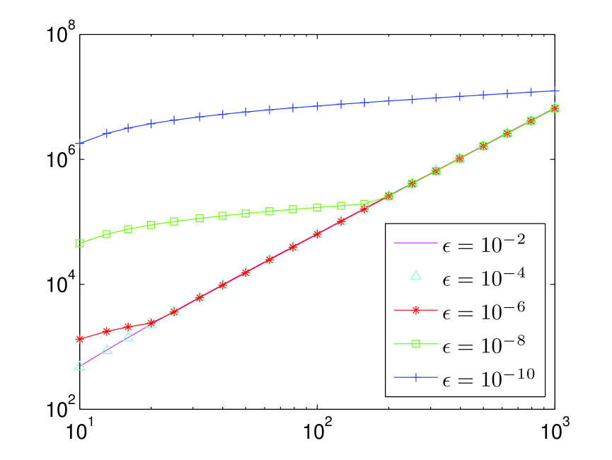
Figure 1: Condition ratio $\kappa=\kappa^{(w)}(N)$ for the dynamic system based on $w$ variable and different values of the regularization parameter $\varepsilon$. The case of the uniform mesh is analyzed.

Influence of the value of $\varepsilon$ on the condition ratio is analyzed in Fig. 1. As an example, we present here the benchmark $q_{l}^{(1)}$ for $Q_{l}/q_{0}=0.9$ (see Appendix C). The results were obtained for the uniform mesh. For other combinations of the benchmark solutions and different meshes the graphs have similar character. As anticipated, the estimation (69) holds true only for sufficiently large $N$. The threshold value of $N$ depends on the chosen $\varepsilon$. Thus for a fixed number of grid points $N$, there is a critical value of the regularization parameter $\varepsilon_{s}(N)$ for which the stiffness characteristics changes its behaviour. By taking $\varepsilon<\varepsilon_{s}(N)$ one increases appreciably the system stiffness.

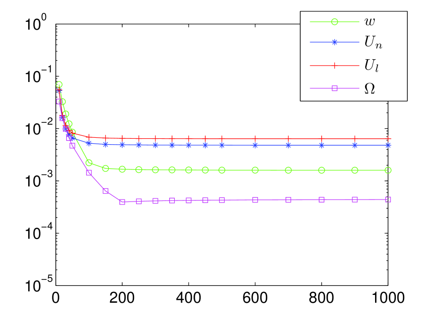
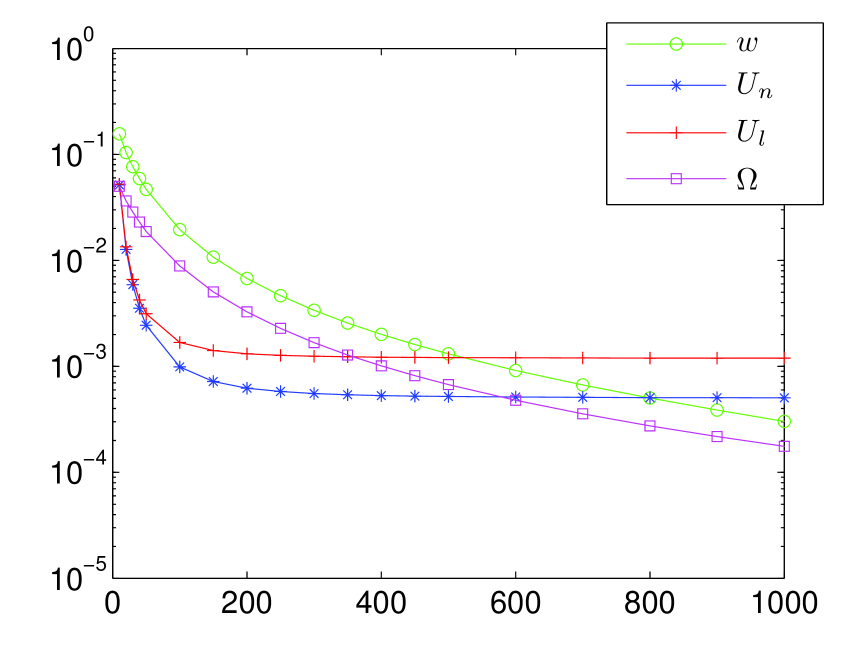
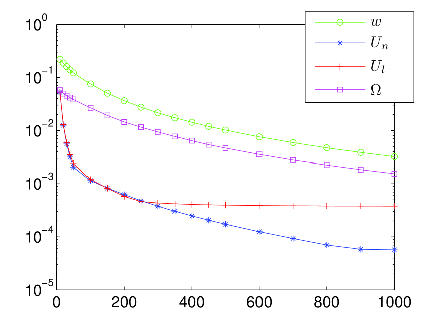
Figure 2: Maximal relative errors of the solutions computed in different variables $\delta w$, $\delta U$ and $\delta\Omega$, for various number of the grid points $N$ in case of the nonuniform mesh $x^{(II)}$ ($\delta=2$). Different values of $\varepsilon$ have been considered. All computations were performed for the benchmark $q_{l}^{(1)}$ for $Q_{l}/q_{0}=0.9$. Solutions $U_{l}$ and $U_{n}$ obtained by unitization of the linear and nonlinear regularized conditions (65) and (66), respectively

The results of the stiffness investigation are collected in the Table 1 and Fig. 1 The following conclusions can be drawn from this data:

• The nonuniform mesh reduces the stiffness approximately up to five times regardless of the solution type (Table 1);

• The most important parameter affecting the stiffness properties is the relation between the injection flux rate and the leak-off to the formation $Q_{l}/q_{0}$ as can be clearly seen in Table 1. The value of this parameter is more important than a particular distribution of the leak-off function (and its behaviour near the crack tip);

• When comparing systems for various dependent variables, the lowest condition ratio gives the system built for $U$ (one order of magnitude lower than the others). The worst stiffness performance takes place for the system corresponding to the $\Omega$-variable. However, in some cases $\Omega$ may produce lower stiffness than $w$;

• A value of the regularization parameter $\varepsilon$ essentially affects the stiffness of a dynamic system.

3.4 Accuracy of the computations

In this section, we analyze the accuracy of computations by the solvers based on different dynamic systems corresponding to the respective dependent variables. To solve the systems, we use MATLAB ode15s subroutine utilizing a version of the Runge-Kutta method dedicated for stiff dynamic systems.

Before we compare different approaches in terms of their accuracy, let us recall two alternative ways to define the regularized boundary condition at the end point $x=1-\varepsilon$. The first one is based on the $\varepsilon$-regularization technique, as it was defined in Linkov (2011d) (see also Mishuris et al. (2012)). The second approach to formulate the regularized condition is to take into account the first two terms of asymptotics as described in section 3.1 (compare equations: (62) and (63)). Finally, in the case of $U$, this condition may be implemented in the non-linear form (66). One can expect that the two term conditions would have a clear advantage, at least in cases when the solution smoothness near the crack tip deteriorates due to the singularity of the leak-off function.

The results of the computations presented in Table 2 confirm such a prediction. We compare only conditions for $U$, as originally the $\varepsilon$-regularization technique was introduced for this variable. Indeed, the relative errors of the solutions $\delta U_{l}$ or $\delta U_{n}$ are at least one order of magnitude lower than that in the case of $\delta U_{*}$, corresponding to the formulation based on (58). Surprisingly, for the variants of the non-singular leak-off function, the improvement is even more pronounced (especially for a uniform mesh).

		Comparison of conditions (58), (65), (66)
		$q_{l}^{(1)}\quad Q_{l}/q_{0}=0.9$			$q_{l}^{(3)}\quad Q_{l}/q_{0}=0.5$
	$\varepsilon=$	$10^{-2}$	$10^{-4}$	$10^{-6}$	$10^{-2}$	$10^{-4}$	$10^{-6}$
$\delta U_{*}$	$x^{(I)}$	1.6e-1	1.4e-1	1.3e-1	6.1e-3	3.7e-3	3.7e-3
	$x^{(II)}$	1.4e-1	7.6e-2	6.3e-2	4.5e-3	9.3e-5	8.9e-5
$\delta U_{l}$	$x^{(I)}$	5.0e-2	1.4e-2	1.7e-2	1.2e-5	1.1e-5	1.1e-5
	$x^{(II)}$	5.0e-2	1.7e-3	2.0e-3	4.9e-5	8.2e-5	8.7e-5
$\delta U_{n}$	$x^{(I)}$	4.4e-2	1.2e-2	1.3e-2	2.2e-5	1.3e-5	1.3e-5
	$x^{(II)}$	4.4e-2	9.9e-4	1.8e-3	4.2e-5	8.2e-5	8.7e-5

Table 2: Comparison of the accuracy of the solution of dynamical system based on variable $U$. The results depicted by $U_{*}$ refer to the regularized boundary condition based on one asymptotic term, while those denoted by $U_{l}$ and $U_{n}$ correspond to two terms approximation (linear (65) and nonlinear (66), respectively). Other problem parameters: $N=100$, $\delta=2$ for the mesh $x^{(II)}$.

We also made the computations for three different benchmarks reported in Mishuris et al. (2012). They correspond to the leak-off function vanishing near the crack tip. It turned out that computational error corresponding to the modified form of the regularized conditions (based on two terms of asymptotics) was always two orders of magnitude lower than that reported in the previous paper.

On the other hand, there is no difference observed between the solutions $\delta U_{l}$ but $\delta U_{n}$ at least for those two benchmarks and the choice of the parameters ($N=100$). However, as we will show later, for large numbers of nodal points, or more severe leak-off function relationship ($Q_{l}/q_{0}\sim 1$), the nonlinear formulation of the condition clearly manifests its advantage.

From now on only the regularized conditions based on two asymptotic terms (63) will be utilized. Additionally, for variable $U$, two different forms, linear (65) and nonlinear (66), will be adopted. For $w$ and $\Omega$ two formulations, (59) and (60), which are equivalent to the condition (58) could not compete with their more accurate analogue (63) in terms of solution accuracy and will not be considered.

Graphs presented in Fig. 2 illustrate some peculiarities of the computational process. Here, the maximal relative errors of the solutions (over the time and space) as functions of the number of mesh points $N$ ($\delta f=\delta f(N)$), are presented for different variables. The considered benchmark assumes $Q_{l}/q_{0}=0.9$ (see Appendix C). Three different values of the regularization parameter $\varepsilon=10^{-3},10^{-4}$ and $10^{-5}$ were chosen.

In Fig. 2 two basic tendencies can be observed. The first one is the monotonous error decrease with growing $N$, up to some stabilization level. This level is different for different dependent variables and values of $\varepsilon$, and in some cases is reached for $N>1000$ (and thus cannot be identified in the figure). The second trend is discernible when comparing results for different values of $\varepsilon$. Namely, it turns out that for each dependent variable there exists an optimal $\varepsilon$ minimizing the solution error. This value however depends on $N$. It is not a surprise that the optimal stiffness properties and the maximal solution accuracy are not achieved for the same values of the regularization parameter $\varepsilon$. To increase computational accuracy one needs to decrease $\varepsilon$ and increase number of the nodal points $N$. However, both of these leads to increase of the condition ratio.

Note that the relative errors of respective dependent variables cannot be compared directly. Indeed, even if the errors for $w$ and $U$ are interrelated via the evident relationship $\delta U=3\delta w$, their comparison with $\delta\Omega$ necessitates an additional postprocessing of the latter. This process, in turn, may introduce its own error. On the other hand, there exists a common component of the solutions, the crack length $\delta L$, which can be naturally used for such comparison.

		Dynamic system built on the variable $w$
		$Q_{l}/q_{0}=0.9$			$Q_{l}/q_{0}=0.5$
		$q_{l}^{(1)}$	$q_{l}^{(2)}$	$q_{l}^{(3)}$	$q_{l}^{(1)}$	$q_{l}^{(2)}$	$q_{l}^{(3)}$
$\delta w$	$x^{(I)}$	8.5e-3	5.4e-3	5.6e-3	5.2e-3	4.0e-3	3.5e-3
	$x^{(II)}$	2.2e-3	2.6e-3	2.9e-3	1.8e-3	1.9e-3	2.0e-3
$\Delta w$	$x^{(I)}$	7.4e-3	9.1e-3	8.8e-3	4.3e-3	4.6e-3	4.7e-3
	$x^{(II)}$	2.8e-3	3.0e-3	3.2e-3	2.1e-3	2.1e-3	2.2e-3
$\delta L$	$x^{(I)}$	1.2e-3	1.3e-3	1.1e-3	5.2e-3	5.3e-3	5.2e-3
	$x^{(II)}$	4.0e-4	3.8e-4	3.1e-4	1.8e-3	1.8e-3	1.8e-3

Table 3: Performance of the solver based on the dependent variable $w$ for number of nodal points $N=100$ and various benchmarks. Values of the regularized parameter are $\varepsilon=5\cdot 10^{-3}$ and $\varepsilon=10^{-3}$ for the meshes for $x^{(I)}$ and $x^{(II)}$, respectively

		System built on $U_{l}$ and condition (65)
		$Q_{l}/q_{0}=0.9$			$Q_{l}/q_{0}=0.5$
		$q_{l}^{(1)}$	$q_{l}^{(2)}$	$q_{l}^{(3)}$	$q_{l}^{(1)}$	$q_{l}^{(2)}$	$q_{l}^{(3)}$
$\delta U$	$x^{(I)}$	1.4e-2	1.0e-2	1.2e-4	2.0e-3	1.4e-3	1.1e-5
	$x^{(II)}$	1.2e-3	6.0e-4	2.5e-4	2.2e-4	1.7e-4	8.6e-5
$\Delta U$	$x^{(I)}$	7.1e-2	4.4e-2	2.0e-3	6.6e-3	4.5e-3	3.9e-4
	$x^{(II)}$	3.1e-2	2.9e-2	7.9e-3	3.5e-3	3.2e-3	7.9e-4
$\delta L$	$x^{(I)}$	4.4e-4	2.8e-4	4.4e-6	4.3e-4	2.9e-4	5.6e-6
	$x^{(II)}$	2.6e-4	2.4e-4	1.2e-4	9.5e-5	8.3e-5	4.3e-5

Table 4: Numerical results for the system built on the dependent variable $U$ with the linear regularized condition (65) for $N=100$ and different $\varepsilon$ for the uniform and nonuniform meshes ($\varepsilon=10^{-4}$ and $\varepsilon=10^{-5}$, respectively).

		System built on $U_{n}$ and condition (66)
		$Q_{l}/q_{0}=0.9$			$Q_{l}/q_{0}=0.5$
		$q_{l}^{(1)}$	$q_{l}^{(2)}$	$q_{l}^{(3)}$	$q_{l}^{(1)}$	$q_{l}^{(2)}$	$q_{l}^{(3)}$
$\delta U$	$x^{(I)}$	1.2e-2	9.2e-3	4.3e-5	1.9e-3	1.4e-3	1.3e-5
	$x^{(II)}$	1.2e-3	6.0e-4	2.5e-4	2.0e-4	1.7e-4	8.6e-5
$\Delta U$	$x^{(I)}$	6.4e-2	4.1e-2	1.7e-3	6.5e-3	4.4e-3	4.0e-4
	$x^{(II)}$	3.1e-2	2.9e-2	7.9e-3	3.5e-3	3.2e-3	7.9e-4
$\delta L$	$x^{(I)}$	4.1e-4	2.7e-4	1.5e-6	4.2e-4	2.9e-4	6.3e-6
	$x^{(II)}$	2.6e-4	2.4e-4	1.2e-4	9.5e-5	8.3e-5	4.3e-5

Table 5: Results for the solver based on the dependent variable $U$ for nonlinear regularized condition for $N=100$ and various benchmarks. Values of the regularized parameter are $\varepsilon=10^{-4}$ and $\varepsilon=10^{-5}$ for the meshes for $x^{(I)}$ and $x^{(II)}$, respectively

		Dynamic system built on variable $\Omega$
		$Q_{l}/q_{0}=0.9$			$Q_{l}/q_{0}=0.5$
		$q_{l}^{(1)}$	$q_{l}^{(2)}$	$q_{l}^{(3)}$	$q_{l}^{(1)}$	$q_{l}^{(2)}$	$q_{l}^{(3)}$
$\delta\Omega$	$x^{(I)}$	2.5e-3	8.7e-4	3.0e-4	5.6e-4	3.3e-4	4.2e-4
	$x^{(II)}$	2.0e-3	7.3e-4	3.6e-4	4.4e-4	2.7e-4	3.1e-4
$\Delta\Omega$	$x^{(I)}$	9.4e-5	1.7e-5	5.9e-5	1.1e-4	1.3e-4	1.5e-4
	$x^{(II)}$	1.9e-4	2.1e-4	2.3e-4	1.3e-4	1.4e-4	1.4e-4
$\delta L$	$x^{(I)}$	2.7e-6	5.0e-7	1.7e-6	2.1e-5	2.5e-5	2.9e-5
	$x^{(II)}$	5.5e-6	6.2e-6	6.7e-6	2.6e-5	2.7e-5	2.8e-5

Table 6: Computation accuracy for the solver based on the dependent variable $\Omega$ for $N=100$ and $\varepsilon=10^{-2}$ for $x^{(I)}$ and $\varepsilon=5\cdot 10^{-3}$ for $x^{(II)}$.

Below we adopt the following strategy for performance test for different dynamic systems. First, we set the number of nodal points, $N$, to 100. Next, for each of the dependent variables we accept optimal (for $N=100$) values of the regularization parameter $\varepsilon$. It turned out that the optimal $\varepsilon$ differs slightly depending on the type of mesh chosen and the benchmark variant. The general trend for $\varepsilon$ can be identified for different meshes (for $x^{(I)}$ it is always smaller than for $x^{(II)}$). However, the sensitivity to the benchmark type is low. The results of computations described by various accuracy measures are collected in Tables 3 – 6 (the optimal values of $\varepsilon$ are specified in the captions). We present there: the relative error of solution $\delta f$, the absolute error of solution $\Delta f$ and the relative error of the crack length $\delta L$. The following conclusions can be drawn from this data:

• Similarly as in case of the stiffness properties, the solution accuracy is affected more by the value of $Q_{l}/q_{0}$ than by the leak-off function behaviour near the crack tip. There is a trend of simultaneous increase of the ratio $Q_{l}/q_{0}$ and the relative errors of dependent variables $\delta f$. However this tendency is not in place (or may be even reversed) when analyzing $\delta L$.

• In case of the dependent variable $U$, the way in which the regularized boundary condition is introduced (linear or non-linear) does not play an essential role for the benchmarks and ranges of the parameters under consideration in the Tables 3 – 6. However, there are exceptions to this rule. One of them can be seen in Fig. 2c) for large values of $N$, where the non-linear condition proves its superiority. Another case will be presented in the end of this section.

• When comparing the common accuracy parameter $\delta L$, the dynamic system for $\Omega$ gives the best results. The dynamic system for $w$ is the worst performing scheme and comparable to the one for $U$ only in a few cases.

• Since $\Omega$ vanishes near the crack tip faster than other variables, one could expect the worst relative error in this case. Surprisingly, even when contrasting the relative (incomparable) errors of the respective dependent variables with each other, the system for $\Omega$ seems to be the best choice. The advantage of $\Omega$ over $w$ and $U$ is especially pronounced for the benchmarks variants with a higher ratio $Q_{l}/q_{0}$.

• Better solution accuracy is obtained for the non-uniform mesh in almost every case.

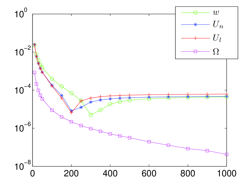
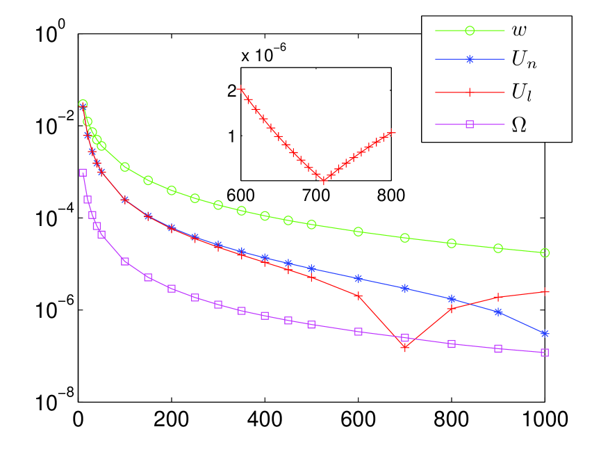
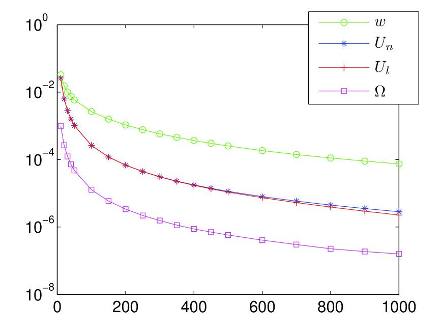
Figure 3: Distribution of relative errors of the fracture length $\delta L$ computed by solvers based on different dependent variables ($w$, $U$ and $\Omega$). When dependent variable $U$ is considered, two different regularised boundary conditions are in use: (65) for $U_{l}$ and (66) for $U_{n}$. Other parameters are the same as in Fig 2. Zoom picture within the Fig. 3 b) corresponds to the sharp minimum of $\delta L$ for the variable $U_{l}$.

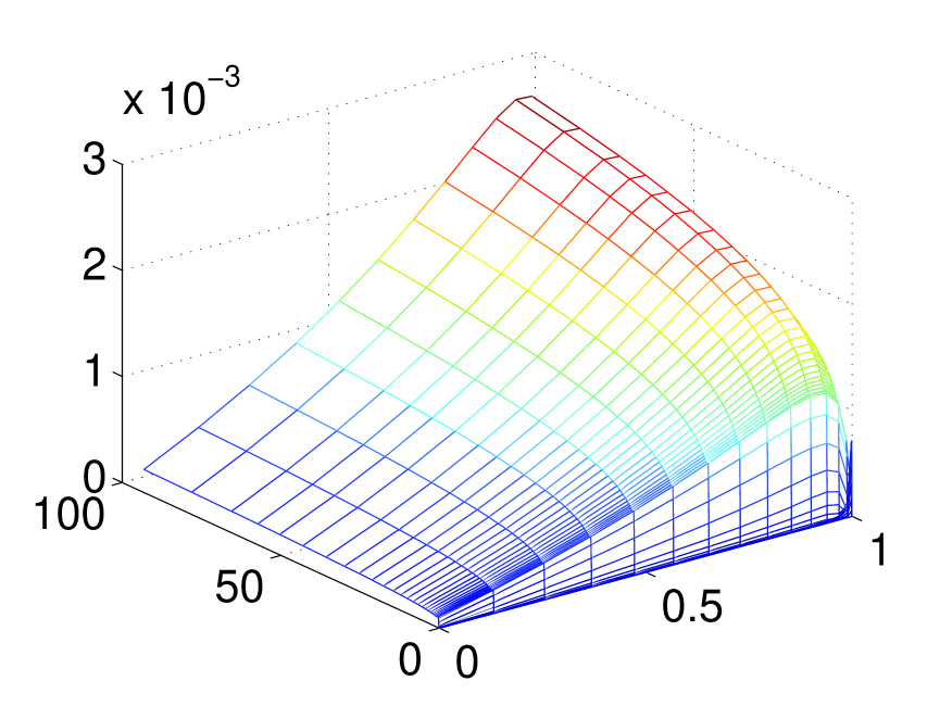
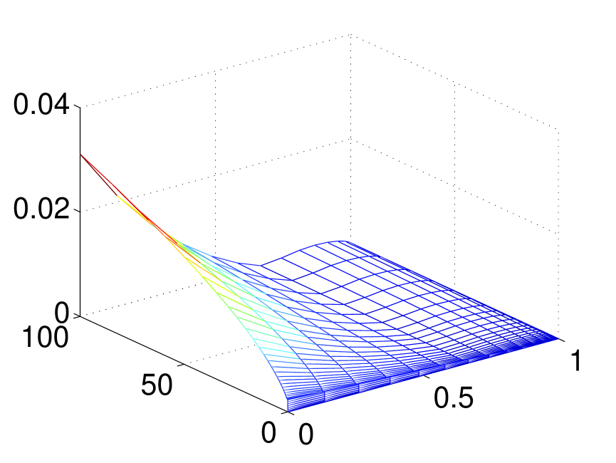
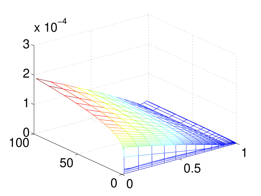
Figure 4: Absolute error for solutions $w$, $U_{n}$ and $\Omega$ computed for benchmark $q_{l}^{(1)}$ with ratio $Q_{l}/q_{0}=0.9$ and nonuniform mesh $x^{(II)}$ ($\delta=2$) with $N=100$ nodal points. Other parameters: $\varepsilon=10^{-3}$ for $w$, $\varepsilon=5\cdot 10^{-3}$ for $\Omega$, and $\varepsilon=10^{-5}$ for $U_{n}$.

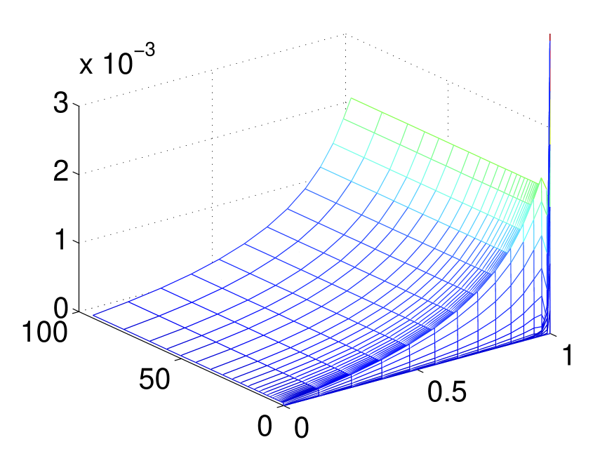
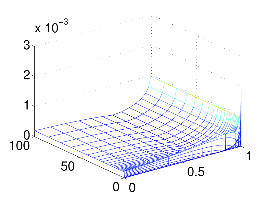
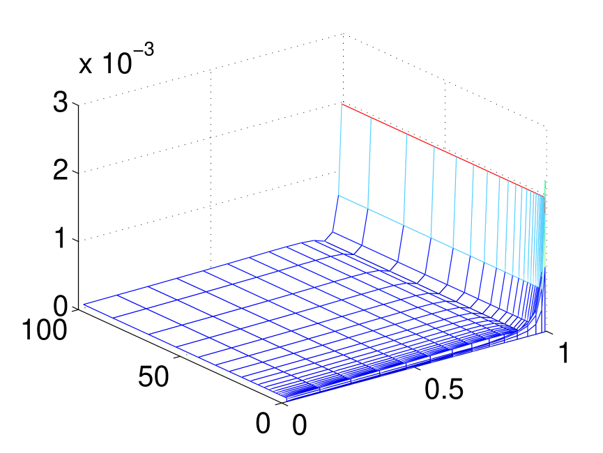
Figure 5: Relative error of the solutions $w$, $U_{n}$ and $\Omega$ computed on the corresponding solvers for the same parameters as in Fig. 4.

We have not observed any significant difference between the time step strategies chosen by the ode15s solver for the different dynamic systems. The number of steps and the main trends were similar. For this reason we have not presented any details in the tables.

To visualize the results reported in the Tables 3 – 6, and to complement those presented in Fig. 2, in Fig. 3 we show the relative errors of the crack length $\delta L$ computed by different dynamic systems (built on different variables). The same benchmark and the values of all other problem parameters as previously discussed in Fig. 2 were considered. If the trends for the different relative errors of the solution $\delta f$ and the crack length $\delta L$ in case of $\varepsilon=10^{-3}$ look similar, the results for the smaller value of the parameter are rather surprising. Indeed, the relative errors $\delta U_{l}$ and $\delta U_{n}$ are smaller than $\delta w$ and $\delta\Omega$, while the error $\delta L$ computed for $U$ no longer follows this trend.

This paradox needs an explanation. A trivial one could be that the maximal error for the solution ($\delta f$) is not situated near the crack tip but inside the computational domain. To verify this hypothesis and to give a prospective reader a clear picture of the distribution of the solution error in time and space, we present, in Fig. 4 and Fig. 5, the corresponding absolute and relative errors computed for the nonuniform mesh built on $N=100$ nodal points with the corresponding optimal regularized parameters discussed after Fig. 2. As it follows from Fig. 5, the maximum of the relative error is always achieved near the crack tip ($\max_{t}\delta f(t,1-\varepsilon))$). Hence, the initial guess has not been confirmed. On the other hand, the values of the relative errors $\delta f$ and the respective $\delta L^{(f)}$ are directly interrelated. The following analysis identifies this relationship.

	$\varepsilon=10^{-2}$		$\varepsilon=10^{-3}$		$\varepsilon=10^{-4}$		$\varepsilon=10^{-5}$
	$x^{(I)}$	$x^{(II)}$	$x^{(I)}$	$x^{(II)}$	$x^{(I)}$	$x^{(II)}$	$x^{(I)}$	$x^{(II)}$
$\delta w$	1.6e-2	1.6e-2	3.4e-2	2.5e-3	6.8e-2	2.1e-2	–	8.2e-2
$\delta U_{l}$	1.9e-1	1.9e-1	8.2e-2	8.1e-2	1.0e-1	4.3e-2	1.5e-1	2.3e-2
$\delta U_{n}$	4.8e-2	4.8e-2	1.1e-2	6.3e-3	1.9e-2	3.2e-3	2.0e-2	9.1e-3
$\delta\Omega$	2.6e-3	5.0e-3	3.0e-3	1.7e-3	3.9e-3	9.9e-3	4.0e-3	3.0e-2
$\delta L_{w}$	2.0e-4	2.6e-4	2.0e-3	1.8e-4	3.4e-3	3.9e-4	–	6.2e-4
$\delta L_{l}$	1.2e-3	1.1e-3	2.7e-4	1.3e-4	7.5e-4	2.8e-4	1.0e-3	3.2e-4
$\delta L_{n}$	2.5e-4	1.2e-4	1.8e-4	2.6e-4	2.5e-4	3.0e-4	2.6e-4	3.2e-4
$\delta L_{\Omega}$	8.1e-7	4.7e-7	1.1e-6	1.1e-6	1.2e-6	1.2e-6	1.2e-6	1.2e-6

Table 7: Accuracy parameters for the limiting (critical) variant of the benchmark solution ($Q_{l}/q_{0}=0.9857$, $\gamma_{v}=2.07$) computed for different meshes composed of $N=100$ nodal points. The blank positions in the table correspond to the case when the solver ode15s could not complete the computations in a reasonable time.

Using (62), after some algebra, one has the estimate:

$$\delta f\approx\delta e_{1}^{(f)}+(\delta e_{2}^{(f)}-\delta e_{1}^{(f)})\frac{e_{2}^{(f)}}{e_{1}^{(f)}}\varepsilon^{\alpha_{2}-\alpha_{1}}.$$ (70)

For the benchmark $q_{l}^{(1)}$ and $Q_{l}/q_{0}=0.9$ (see Appendix C) which always provides the worst accuracy in our computations, one can conclude

$$\delta w\approx\frac{1}{3}\delta U\approx\delta w_{0}+\frac{1}{10}(\delta w_{1}-\delta w_{0})\sqrt[6]{\varepsilon},$$ (71)

$$\delta\Omega\approx\delta w_{0}+\frac{8}{90}(\delta w_{1}-\delta w_{0})\sqrt[6]{\varepsilon}.$$ (72)

Finally, from (31) we can derive

$$\delta L\approx\frac{3}{2}\delta w_{0}.$$ (73)

The last relationship has also been verified numerically by evaluating the values of the constant $w_{0}$ in the postprocessing procedure using the computed solution ($w$, $U$ or $\Omega$) and the corresponding regularized boundary condition (compare (62) and (63)).

It is clear from relations (71) – (72) that the relative errors of the respective dependent variables also depend on the quality of approximation of the second term in the regularized boundary condition (62). This explains the surprising relationship between $\delta L$ and the respective $\delta f$.

Interestingly, the results presented in Fig. 3 show that the value of $\varepsilon$ which provides the lowest relative error, $\delta f$, of the dependent variable $f$ does not necessarily give the best accuracy of the crack length $\delta L$. Moreover, the relation $\varepsilon=\varepsilon_{L}(N)$ is much more sensitive to the variation of $N$ than $\varepsilon=\varepsilon_{f}(N)$. Indeed, one can observe sharp minima (see Fig. 3 a) and b)) while there is no such phenomenon in the respective graphs for $\delta f$ (see Fig. 2). To demonstrate that the peaks are not computational artifacts, we also include a small zoom of the corresponding area of the figure Fig. 3 b).

To complete the accuracy analysis, let us consider some critical regime of crack propagation. Namely, assume that the leak-off flux almost entirely balances the volume of fluid injected into the crack. Indeed, when taking the Carter type benchmark (91) $b_{1}=b_{2}=1$, one obtains the fluid balance ratio $Q_{l}/q_{0}=0.9857$. This gives a very strong variation of the particle velocity function along the crack length ($\gamma_{v}=2.07$ - see (95)).

In view of the previous conclusion on the influence of the ratio $Q_{l}/q_{0}$ on the solution accuracy (which in fact confirms the observations from Mishuris et al. (2012)), one can predict that the solution error will increase appreciably in comparison with the figures shown in Tables 3 – 6. In order to verify this assertion the computations were made for respective dynamic systems (the system for $U$ was analyzed again for two forms of the regularized boundary condition). Both types of meshes, the uniform and the non-uniform, were utilized, each composed of 100 nodal points ($N=100$). Four different values of the regularization parameter $\varepsilon$ , ranging from $10^{-5}$ to $10^{-2}$, were analyzed. The results of the computations described by respective accuracy parameters are presented in Table 7. Here, the symbols $\delta U_{l}$ and $\delta U_{n}$ stand for the relative error of $U$ obtained for the conditions (65) and (66), respectively. The subscript of $\delta L$ informs us which dynamic system the corresponding result was obtained for.

The data in the table shows that the solution error increased at least one order of magnitude, as compared to the values from Tables 3 – 6. The lowest deterioration of the solution accuracy was obtained for $\Omega$, which proves the best overall performance of the system built for this variable. Especially impressive is its advantage when comparing the errors of crack length estimation. In all considered cases $\delta L_{\Omega}$ is at least two orders of magnitude lower than $\delta L$ for other dependent variables.

In this critical variant of benchmark solution, the non-linear regularized boundary condition (66) for $U$ gives, in most cases, much better performance than its linear counterpart (65) (compare with the discussion after the Tables 2 and 3 – 6). Finally, the non-uniform mesh seems to be a better choice from the point of view of accuracy.

In the last test in this subsection we discuss the sensitivity of respective algorithms to the variation of the crack propagation regime. To this end, consider again the benchmark solution (90) for the critical value of the ratio $Q_{l}/q_{0}=0.9857$ ($\gamma_{v}=2.07$). Now, we analyze a range of parameters $\gamma>-1/3$, motivated by the physical sense of the solution. By changing this value, one simulates different modes of crack propagation (see Appendix B). The non-uniform mesh composed of 100 nodes nodes was utilized. For each of the dependent variables an optimal value of the regularization parameter, $\varepsilon$, was taken: $\varepsilon=10^{-3}$ for $w$, $\varepsilon=10^{-5}$ for $U$, and $\varepsilon=5\cdot 10^{-3}$ for $\Omega$. The results of the computations illustrated by the relative errors of the crack length and the maximal relative errors of corresponding dependent variables are shown in Fig. 6 – Fig. 7, respectively.

Figure 6: The relative errors of the crack length
for different dependent variables as functions of $\gamma$.

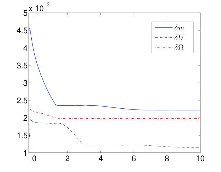
Figure 7: The maximal relative errors of respective dependent variables as functions of $\gamma$.

As can be seen in Fig. 6, for all dependent variables the crack length error rapidly decreases for $\gamma\to-1/3$. Indeed, this is the case when $L(t)\sim L_{0}$. For $w$ and $U$ solvers, $\delta L$ remains very stable over most of the analyzed interval. The solver based on $\Omega$ exhibits quite different behaviour. For $\gamma$ greater than approximately 1.4, the error decreases to achieve the level of its ultimate accuracy, the same as for $\gamma\to-1/3$. Depending on the crack propagation regime, this solver can produce up to two orders of magnitude better accuracy of $L(t)$ than others.

Fig. 7 shows, that respective dependent variables themselves are much less sensitive to the changes of $\gamma$ that the crack length. In the considered interval each solver provides a relatively stable level of accuracy (within the same order of magnitude).

This test proves that using the solver based on $\Omega$ is especially beneficial when dealing with the problems of fast propagating fractures (large values of $\gamma$).

3.5 Comparison with known numerical results.

Although the benchmark solutions utilized in the previous subsections incorporate among others the leak-off term with a square root singularity, there is no analytical solution for the Carter leak-off. In Kovalyshen and Detournay (2009), one can find the numerical results for such a case. This data may be utilized as a reference solution. Unfortunately, the authors provide only some rough estimation of the solution error. Surprisingly, they do not even verify their numerical scheme against the early time asymptotic model (considered as an analytical benchmark) to establish quantitatively the accuracy of computations for the zero leak-off case.

The numerical method used in Kovalyshen and Detournay (2009) is based on an implicit finite volume algorithm. The data collected in their Table 1 (p.332) describes the normalized values of the crack length, the crack propagation speed and the crack opening at $x=0$, at a number of times steps in the interval $t\in[10^{-5},5\cdot 10^{2}]$. There is no precise information on the utilized number of control volumes and the time stepping strategies (the mentioned number of 10 control volumes refers to the presented graphs, but it is not clear if the data from table was obtained for the same parameters).

In the following we compare our numerical solution (see Table 8) with that by Kovalyshen and Detournay (2009). Note that, due to different normalizations, our normalized crack length, $L$, is two times greater than respective value in their paper. Our data was obtained by the solver based on $U$ variable for $N=1000$ nodal points. Although from the previous analysis it emerges that the system for $\Omega$ can provide better accuracy of $L$, we do not use it here to avoid an additional postprocessing (numerical differentiation) when computing $w(0,t)$. On the other hand, in the light of previous investigations, the system for $U$ for $N=1000$ can give the accuracy of $L$ up to $10^{-6}$.

First, we present the graphs for evolution of the crack length, $L(t)$, - Fig. 8, and the crack aperture at zero point, $w(t,0)$ - Fig. 9. They depict the data for early time and large time asymptotic models (respective formulae can be found also in Kovalyshen and Detournay (2009)), and the numerical results for a transient regime connecting these asymptotes. The solution by Kovalyshen and Detournay (2009) is indicated by markers. A figure, equivalent to Fig. 8, has been also published in Nordgren (1972), however there is no data available for comparison.

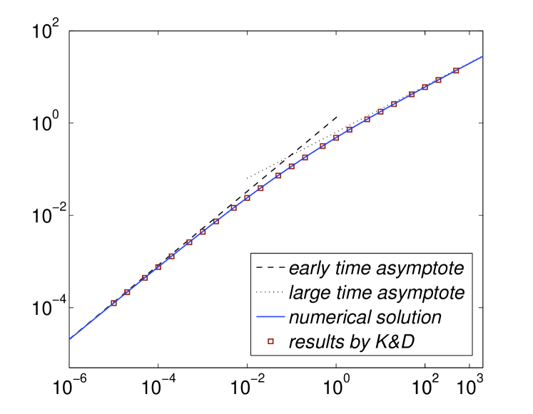
Figure 8: The crack length evolution in time.

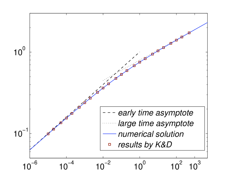
Figure 9: The evolution of crack opening at zero point, $w(t,0)$.

We analyze the time interval $t\in[10^{-8},10^{8}]$ where the initial conditions correspond to the early time asymptote for $t=10^{-8}$. The same initial time was taken by Kovalyshen and Detournay (2009), but the authors presented their data starting from $t=10^{-5}$. In order to increase the legibility of the graphs, we have truncated the time axis to the range $t\in[10^{-6},5\cdot 10^{3}]$, while the complete data is presented in Table 8.

In Fig. 10 we show the normalized crack propagation speed, defined in a manner introduced by Kovalyshen and Detournay (2009).

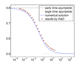
Figure 10: The evolution of the normalized crack propagation speed.

As can be seen in the Fig. 8 – Fig. 9, in the presented scale, our solution is undistinguishable from that by Kovalyshen and Detournay (2009) in terms of $L(t)$ and $w(t,0)$. However, the normalized crack propagation speeds differ appreciably from each other. It shows that our solution fits the asymptotes very well, which suggests its good quality. We cannot examine, how the solution of Kovalyshen and Detournay (2009) approaches the asymptotic values due to the shortage of data for time intervals $t<10^{-5}$ and $t>5\cdot 10^{3}$ in their table.

In the analyzed case, the value of the parameter $Q_{l}(t)/q_{0}(t)$ changes continuously with time from zero to unit. From the data presented in Mishuris et al. (2012) and in this paper, one can conclude that for $N=100$ nodal points, the relative error of the crack length changes from $10^{-6}$ to $10^{-4}$ with the increase of the parameter $Q_{l}/q_{0}$. On the other hand, analyzing the data from Fig. 2 – Fig. 3 ($Q_{l}/q_{0}=0.9$), one can expect the achievable level of accuracy of the order $10^{-7}$ for $N=1000$. This suggests that, in our computations, the relative error of $L$ varies between $10^{-4}$ and $10^{-6}$.

In order to additionally asses the credibility of our solution (computed for $N=1000$ and presented in the Table 8), we show in Fig. 11 the relative deviations between it and other solutions. Namely, we analyze the crack lengths $L$ provided by: a) early and large time asymptotes; b) the solution by Kovalyshen and Detournay (2009); c) the solution obtained for 100 nodal points and d) the solution obtained for 1000 nodal points at another starting point $t_{0}=10^{-7}$.

When tracing the data from Fig. 11 we can see that the deviations of $L$ from the early and large time asymptotes at the ends of the considered interval are of the order $10^{-4}$. Moreover, the relative deviation of the solution obtained for 100 points is of the same order in almost entire time range, which corresponds very well to the figures from Tab 7. The discrepancy between the reference solution and the solution for $t_{0}=10^{-7}$ decreases rapidly with time. The last observation confirms the credibility of the reference solution.

We do not present respective graph for $w(t,0)$. However, it is worth mentioning that in this case the deviations from the asymptotes were even lower than for $L$, while the deviation of the solution for $N=100$ did not exceed the value of $10^{-4}$ on the substantial part of the interval.

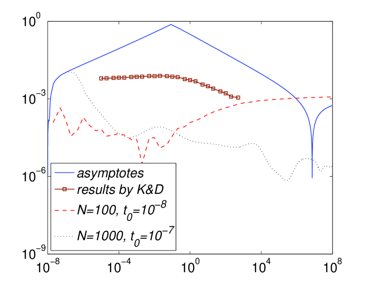
Figure 11: Relative deviations from the numerical
solution for $L$.

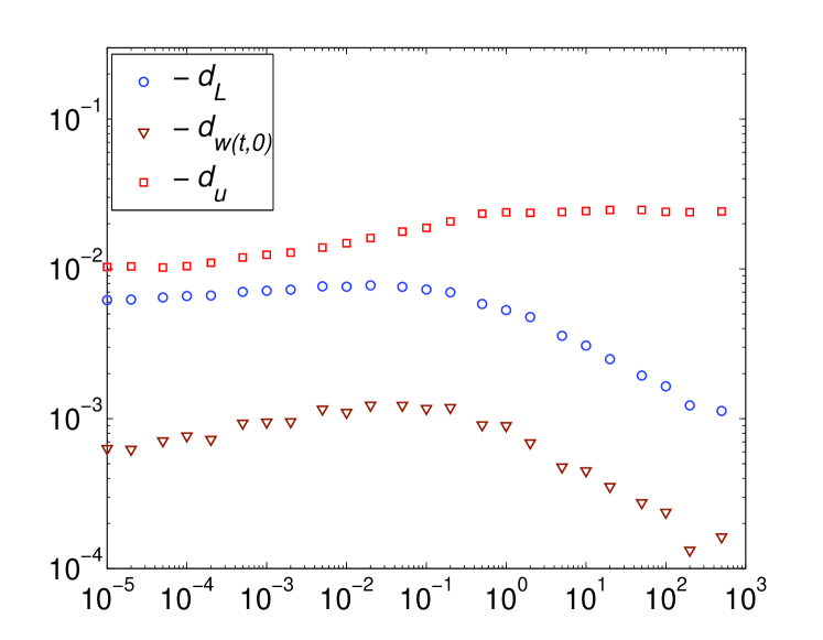
Figure 12: Relative deviations of the solution by Kovalyshen and Detournay (2009) from the results reported in Table 8.

The relative discrepancies between the components of our solution and the solution by Kovalyshen and Detournay (2009) are shown in Fig. 12. Here $d_{L}$, $d_{w(0,t)}$ and $d_{u}$ refer to the deviations of the crack length, $L$, the crack opening, $w(t,0)$ and the normalized crack velocity, $u$, respectively.

In the light of the presented results, we believe that the data collected in Table 8 provide the accuracy at least of the order $10^{-4}$ for both, the crack length, $L$, and the crack opening at $x=0$. Moreover, in the considerable time range ($10^{-6}<t<10^{6}$), one can expect the error lower by up to two orders of magnitude. The normalized crack propagation speed $u$ is computed with accuracy of one to two orders of magnitude lower.

Summarizing the above discussions, the level of accuracy for the results tabulated by Kovalyshen and Detournay (2009) can be estimated as $10^{-3}\div 10^{-2}$ for $L$, $10^{-4}\div 10^{-3}$ for $w(t,0)$ and of the order $10^{-2}$ for $u$.

$\log(t)$	$L(t)$	$w(t,0)$	$u(t)\times 10$
$-7$	3.283747e-6	3.988347e-2	7.9701
$-6$	2.049209e-5	6.298786e-2	7.9355
$-5$	1.265786e-4	9.915967e-2	7.8716
$-4$	7.660018e-4	1.551088e-1	7.7536
$-3$	4.456291e-3	2.397462e-1	7.5185
$-2$	2.412817e-2	3.629593e-1	7.1173
$-1$	1.163591e-1	5.326638e-1	6.5267
$0$	4.849863e-1	7.541837e-1	5.8885
$1$	1.779508e0	1.037495e0	5.4408
$2$	6.035529e0	1.403522e0	5.1993
$3$	1.968511e1	1.883411e0	5.0847
$4$	6.308563e1	2.518338e0	5.0378
$5$	2.006370e2	3.362113e0	5.0146
$6$	6.360179e2	4.485636e0	5.0071
$7$	2.013373e3	5.982935e0	5.0029

Table 8: Numerical solution of the PKN fracture.

3.6 Remarks on the sensitivity of the Carter leak-off model.

It is well known that applicability of the empirical Carter law (4)₁ in the vicinity of the fracture tip is questionable (see for example, Economides (2000), Kovalyshen (2010) and Mitchell et al. (2007)). Moreover, when combining Carter’s leak-off with some non-local variants of elasticity models (for example, KGD model of hydrofracturing), one obtains an infinite particle velocity at the crack tip. As a result, the speed equation (12) cannot be applied in such a case. One of the ways to eliminate the negative consequences of this fact is to assume that the Carter law becomes valid at some distance away from the fracture tip (see for example Mitchell et al. (2007)).

The PKN model, which does not exhibit such a drawback, gives however a unique opportunity to assess how the solution is affected by a modification of the classic Carter law in the neighborhood of the fracture tip.

To this end, let us consider two ways of modification of the law. The first one assumes that leak-off function equals zero over some distance from the crack front ($d>\varepsilon$). The second one accepts a constant value of $q_{l}$ in the same interval. This value is taken in such a manner to preserve the continuity of the leak-off function. Note, that both of these modifications change the volume of fluid loss to the rock formation, with respect to the original state.

The relative deviations of the crack lengths for these modifications from the original one are shown in Fig. 13. Results for two values of $d$: $d=\varepsilon$, $d=10\varepsilon$ (for $\varepsilon=10^{-5}$) are depicted. The symbol $q_{ld}$ in the legend refers to the cases when the leak-off function is complimented by the constant value over $1-d\leq x\leq 1$.

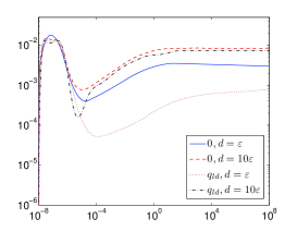
Figure 13: Relative deviations of the crack lengths for different variants of truncated Carter law.

One can see from this picture that the maximal relative discrepancies (of the level of 1%) appear at the initial and large time ranges. To explain this phenomenon we can easily compute the additional volume of fluid retained in the fracture as a result of the Carter law amendments. Taking into account (74), these values are $\Delta Q_{l}(t)=2D(t)\sqrt{d}$ and $\Delta Q_{l}(t)=D(t)\sqrt{d}$, for the respective modifications (see (22) for $D(t)$). Note that $D(t)=\sqrt{u(t)/t}$, which explains the level of deviation for the small time. For large time, the effect of accumulation of the difference of the fluid loss, $\int_{0}^{t}\Delta Q_{l}(\tau)d\tau$ = $O(\sqrt{td})$, plays a crucial role.

The above test proves that the application of the Carter law modified in the aforementioned ways, is acceptable in terms of both the stability and the accuracy of computations. This allows one to use such an approach in the cases when the law leads to unphysical results (see Mitchel et al. 2007). Note, however, that the intermediate asymptotics related to the carter law still holds true and thus should be taken into account.

On the other hand, appreciable sensitivity of the solution to the slight modifications of the Carter law calls the validity of the law near the crack tip into question.

4 Conclusions

In this paper, we have revisited the PKN model of hydrofracturing providing a comprehensive overview of the known results together with:

• analysis of various leak-off regimes (vanishing, bounded and singular near the fracture tip) supplemented with the full asymptotic expansion of the solution for the Carter model;

• introduction of a new dependent variable, $\Omega$, and the resulting problem reformulation;

• implementation of a new form of the regularized boundary condition;

• analysis of different aspects of application of various dependent and independent variables, including the stiffness properties, accuracy and efficiency of the computations;

• comparison of the results for the Carter leak-off with the known numerical benchmark from Kovalyshen and Detournay (2009).

The main conclusions of the paper are:

• The approach proposed in Linkov (2011d); Mishuris et al. (2012) is efficient even in the cases when the smoothness of the particle velocity near the crack tip is disturbed by the singular leak-off function;

• For the best performance of a solver, the regularized boundary condition should incorporate at least two leading terms of asymptotics;

• The stiffness properties of the dynamic systems and the accuracy of the computations can be effectively controlled by the choice of dependent and independent variables.

• The new independent variable, $\Omega$, leading to a slightly greater stiffness of the dynamic system, considerably improves the accuracy of computations.

The value of the aforementioned findings was demonstrated on various analytical benchmarks and for the classic Carter law. Although, the presented analysis concerns the 1-D PKN formulation, at least some of the findings may be utilised in the more advanced cases.

Appendices

Appendix A Carter’s leak-off function in the normalised formulation

Consider the transformation of the Carter law described by (4) when applying the normalization (18). Assume that:

$$\frac{1}{\sqrt{t-\tau(x)}}=\frac{D(t)}{\sqrt{1-\tilde{x}}}+R(t,\tilde{x}),$$ (74)

where function $D(t)$ is defined in (22) while the remainder $R$ is estimated later in (77).

To find function $D(t)$, and thus to obtain an exact form of equation (22), it is enough to compute the limit

$$D^{2}(t)=\lim_{\tilde{x}\rightarrow 1}\frac{1-\tilde{x}}{t-\tau(x)}.$$ (75)

This can be done by utilising L’Hopital’s rule with taking into account that $x\to L(t)$ as $\tilde{x}\rightarrow 1$,

$$\tau(x)=\tau\left(L(t)\tilde{x}\right)=L^{-1}(L(t)\tilde{x}),$$ (76)

and that the crack length is a smooth function of time ($L\in C^{1}$ at least). The last fact immediately follows from the problem formulation in terms of evolution system (32).

Having the value of $D(t)$ we can estimate the remainder $R(t,\tilde{x})$ when $\tilde{x}\to 1$, or, what it is equivalent to when $x\to l(t)$ (or $t\to\tau(x)$). For this reason, we search for a parameter $\xi\neq 0$ which guarantees that the limit

$$A=\lim_{\tilde{x}\rightarrow 1}\frac{R(t,\tilde{x})}{(1-\tilde{x})^{\xi}}=\lim_{\tilde{x}\rightarrow 1}\frac{1}{2\xi(1-\tilde{x})^{\xi-1}}\left(\frac{D(t)}{(1-\tilde{x})^{3/2}}-\frac{L(t)\tau^{\prime}(x)}{(t-\tau(x))^{3/2}}\right)$$

does not turn to zero or infinity. Due to this assumption, we can write

$$\frac{1}{\sqrt{t-\tau(x)}}=\frac{D(t)}{\sqrt{1-\tilde{x}}}+A(1-\tilde{x})^{\xi}+o\left((1-\tilde{x})^{\xi}\right),$$ (77)

when $\tilde{x}\rightarrow 1$, or equivalently $x\rightarrow l(t)$. Taking the last estimate into account $A$ can be expressed as:

$$A=\lim_{\tilde{x}\rightarrow 1}\frac{1}{2\xi(1-\tilde{x})^{\xi-1}}\left(\frac{D(t)}{(1-\tilde{x})^{3/2}}-\frac{L(t)\tau^{\prime}(x)}{t-\tau(x)}\frac{D(t)}{\sqrt{1-\tilde{x}}}\right)-\frac{AL(t)}{2\xi}\lim_{\tilde{x}\rightarrow 1}\frac{(1-\tilde{x})\tau^{\prime}(x)}{t-\tau(x)}\big{(}1+o(1)\big{)}.$$

Now, on substitution of $\tau^{\prime}(x)=1/L^{\prime}(t)$ at $x=L(t)$ and (75) into the limit one has:

$$A=\lim_{\tilde{x}\rightarrow 1}\frac{D(t)}{2\xi(1-\tilde{x})^{\xi-1/2}}\left(\frac{1}{1-\tilde{x}}-\frac{L(t)\tau^{\prime}(x)}{t-\tau(x)}\right)-\frac{AL(t)D^{2}(t)}{2\xi L^{\prime}(t)}.$$

Applying (75) and (22) here gives:

$$\frac{1+2\xi}{2\xi}A=\lim_{\tilde{x}\rightarrow 1}\frac{D(t)}{2\xi(1-\tilde{x})^{\xi-1/2}}\left(\frac{1}{1-\tilde{x}}-\frac{L(t)\tau^{\prime}(x)}{\sqrt{t-\tau(x)}}\frac{D(t)}{\sqrt{1-\tilde{x}}}\right)-\frac{AD(t)L(t)}{2\xi}\lim_{\tilde{x}\rightarrow 1}\frac{\tau^{\prime}(x)\sqrt{1-\tilde{x}}}{\sqrt{t-\tau(x)}}.$$

By repeating the same process one more time we have:

$$(2+2\xi)A=\lim_{\tilde{x}\rightarrow 1}\frac{D(t)}{(1-\tilde{x})^{\xi}}\left(\frac{1}{\sqrt{1-\tilde{x}}}-\frac{L(t)\tau^{\prime}(x)D(t)}{\sqrt{t-\tau(x)}}\right).$$

Finally by eliminating the square root with use of (77) we obtain (after some algebra)

$$(3+2\xi)A=D(t)\lim_{\tilde{x}\rightarrow 1}\frac{1-L(t)\tau^{\prime}(x)D^{2}(t)}{(1-\tilde{x})^{\xi+1/2}}.$$

This relationship gives a finite value of $A$ if and only if $\xi=1/2$ and, as a result, we find:

$$A=\frac{1}{4}D^{3}(t)L^{2}(t)\tau^{\prime\prime}(L(t))=-\frac{1}{4}\frac{L^{\prime\prime}(t)}{L^{\prime}(t)}\sqrt{\frac{L(t)}{L^{\prime}(t)}}.$$

Appendix B Asymptotics of the solutions for different leak-off functions

Asymptotic expansion for the crack opening and the fluid velocity near the crack tip in the normalised variables (18) can be written in the following general forms:

$$w(t,x)=\sum_{j=0}^{N}w_{j}(t)(1-x)^{\alpha_{j}}+O((1-x)^{\varrho_{w}}),\quad x\rightarrow 1,$$ (78)

and

$$V(t,x)=\sum_{j=0}^{N}V_{j}(t)(1-x)^{\beta_{j}}+O((1-x)^{\varrho_{V}}),\quad x\rightarrow 1,$$ (79)

with $\varrho_{w}>\alpha_{n}$, $\varrho_{V}>\beta_{n}$, $\alpha_{0}=1/3$, $\beta_{0}=0$ and some increasing sequences $\alpha_{0},\alpha_{1},\ldots,\alpha_{n}$ and $\beta_{0},\beta_{1},\ldots,\beta_{n}$. Note that the asymptotics are related to each other by the speed equation (19) and thus, regardless of the chosen leak-off function, we can write

$$\sum_{j=0}^{N}V_{j}(t)(1-x)^{\beta_{j}}+\ldots=\frac{1}{3L(t)}\sum_{k=0}^{N}\sum_{m=0}^{N}\sum_{j=0}^{N}\alpha_{j}w_{j}(t)w_{m}(t)w_{k}(t)(1-x)^{\alpha_{j}+\alpha_{m}+\alpha_{k}-1}.$$ (80)

In line with the discussion after equation (16), we are interested only in the terms such that $\beta_{j}\leq 1$, restricting ourselves to the smallest $\varrho_{V}>1$, since the values of $\beta_{j}$ are combinations of a sum of three consequent components of the exponents $\alpha_{j}$. However, since $\alpha_{0}$ is known ($\alpha_{0}=1/3$), one can write (compare with (17)):

$$V_{0}(t)=\frac{1}{3L(t)}w_{0}^{3}(t),$$ (81)

$$V_{1}(t)=\frac{1}{L(t)}\left(\alpha_{1}+\frac{2}{3}\right)w_{0}^{2}(t)w_{1}(t),\quad\beta_{1}=\alpha_{1}-\frac{1}{3}.$$ (82)

To continue the process one now needs to compute the value of the exponent $\alpha_{1}$ as it is not clear a priori which value determining the next exponent $\beta_{2}=\min\{2/3+\alpha_{2},1/3+2\alpha_{1}\}$ is larger. To do so let us rewrite the continuity equation (20) in the form:

$$\frac{\partial w}{\partial t}+\frac{V_{0}(t)}{L(t)}(1-x)\frac{\partial w}{\partial x}=\frac{1}{L(t)}\frac{\partial\big{(}w(V_{0}-V)\big{)}}{\partial x}-q_{l}(t,x).$$ (83)

Here, the terms on the left-hand side of the equation are always bounded near the crack tip, while those on the right-hand side can behave differently depending on the chosen leak-off function.

Consider the following three cases of $q_{l}$ behaviour.

(i) Assume first that

$$q_{l}(t,x)=o\big{(}w(t,x)\big{)},\quad x\to 1.$$

This case naturally includes the impermeable rock formation. Analysing the leading order terms in the equation (83), it is clear that $w(V_{0}-V)=O((1-x)^{4/3})$, as $x\to 1$. This, in turn, is only possible for $\beta_{1}=1$ and, therefore, $\alpha_{1}=4/3$. Finally, comparing the left-hand side and the right-hand side of the equation we obtain:

$$w_{0}^{\prime}(t)=\frac{w_{0}(t)}{3L(t)}\big{(}V_{0}(t)+4V_{1}(t)\big{)},\quad V_{1}(t)=\frac{2}{L(t)}w_{0}^{2}(t)w_{1}(t).$$ (84)

This case has been considered in Linkov (2011d) and Mishuris et al. (2012).

(ii) If we assume that the leak-off function is estimated by the solution as $O\big{(}w(t,x)\big{)}$, or equivalently;

$$q_{l}(t,x)\sim\Upsilon(t)w_{0}(t)(1-x)^{1/3},\quad x\to 1,$$

then the previous results related to the values of $\alpha_{1}$ and $\beta_{1}$ and, therefore, the equation (84)₂ remain the same, while the first one changes to

$$w_{0}^{\prime}(t)=\frac{1}{3L(t)}w_{0}(t)\big{(}V_{0}(t)+4V_{1}(t)\big{)}-\Upsilon(t)w_{0}(t).$$ (85)

This case corresponds to (21)₃ when $C_{32}=0$ and $\Upsilon(t)=kC_{31}(t)$.

(iii) The leak-off function in a general form:

$$q_{l}(t,x)=\Phi(t)(1-x)^{\theta}+o((1-x)^{1/3}),\quad x\to 1,$$

where $-1/2\leq\theta<1/3$. Here, one can conclude that $w(V_{0}-V)=O((1-x)^{1+\theta})$, as $x\to 1$ or equivalently, $\beta_{1}=\theta+2/3$, and $\alpha_{1}=1+\theta$. Moreover, in this case:

$$(1+\theta)w_{0}V_{1}=L(t)\Phi(t),\quad V_{1}(t)=\frac{1}{L(t)}\left(\theta+\frac{4}{3}\right)w_{0}^{2}(t)w_{1}(t),$$ (86)

and, thus

$$w_{1}(t)=\frac{3L^{2}(t)\Phi(t)}{(4+3\theta)(1+\theta)w_{0}^{3}(t)}.$$ (87)

Note, that as one would expect, the particle velocity function is not smooth in this case near the crack tip, its derivative is unbounded and exhibits the following behaviour:

$$\frac{\partial V}{\partial x}=O\big{(}(1-x)^{\theta-1/3}\big{)},\quad x\to 1.$$

To formulate the equation similar to (84)₁ or (85), one needs to continue asymptotic analysis of the equation (83) incorporating the available information. Apart from the fact that the analysis can be done in the general case, we restrict ourselves only to three variants used from the beginning (compare (4)), respectively: $\theta=0$, $\theta=1/3-1/2=-1/6$ and $\theta=-1/2$.

When $\theta=0$, $\alpha_{1}=1$ and $\beta_{1}=2/3$, returning to the equation (80), one concludes that $\beta_{2}>1$ and, therefore,

$$w_{0}^{\prime}(t)=\frac{1}{3L(t)}w_{0}(t)V_{0}(t).$$ (88)

This case corresponds to (21)₃ when $\Phi(t)=C_{3}^{(2)}(t)w_{0}(t)$ and $C_{3}^{(1)}=0$.

If $\theta=-1/6$, then $\alpha_{1}=5/6$ and $\beta_{1}=1/2$. In this case the function $\Phi(t)$ can be written as $\Phi(t)=C_{2}D(t)w_{0}(t)$ (compare to (21)₂) and again equation (80) gives $\beta_{2}>1$, while equation (83) leads to

$$w_{0}^{\prime}(t)=\frac{1}{3L(t)}\big{(}w_{0}(t)V_{0}(t)+4w_{1}(t)V_{1}(t)\big{)}.$$ (89)

Summarizing, in both mentioned above cases, there exists a single term in asymptotics of the particle velocity which has singular derivative near the crack tip. Moreover, those terms ($w_{1}$ and $V_{1}$, respectively) are fully defined by the leak-off function $\Phi(t)$ and the coefficient $w_{0}$ in front of the leading term for the crack opening in (87) and (86)₁.

The situation changes dramatically when $\theta=-1/2$ (Carter law). We now have $\alpha_{1}=1/2$ and $\beta_{1}=1/6$ and $\Phi(t)=C_{1}D(t)$. In this case, however, $\beta_{2}<1$ and we need to continue the asymptotic analysis further to evaluate all terms of the particle velocity which exhibit non-smooth behaviour near the crack tip. We omit the details of the derivation, presenting only the final result in a compact form. The first six exponents in the asymptotic expansions (78) and (79), that introduce the singularity of $w_{x}$, are:

$$\alpha_{j}=\frac{1}{2}+\frac{j}{6},\quad\beta_{j}=\frac{j}{6},\quad j=1,2,\ldots,6.$$

$$w_{j}(t)=\kappa_{j}\frac{\Phi^{j}(t)L^{2j}(t)}{w_{0}^{4j-1}(t)},\quad V_{j}(t)=\psi_{j}\frac{\Phi^{j}(t)L^{2j-1}(t)}{w_{0}^{4j-3}(t)},$$

where $j=1,2,\ldots,5$ and

$$\begin{array}[]{l}\kappa_{1}=\frac{12}{7},\quad\psi_{1}=2,\quad\kappa_{2}=-\frac{270}{49},\quad\psi_{2}=-\frac{24}{7},\kappa_{3}=\frac{9768}{343},\,\,\psi_{3}=\frac{828}{49},\\[11.38109pt] \kappa_{4}=-\frac{2097252}{12005},\,\,\psi_{4}=-\frac{5136}{49},\,\,\kappa_{5}=\frac{1081254096}{924385},\quad\psi_{5}=\frac{1234512}{1715}.\end{array}$$

Appendix C Benchmark Solutions

There are several benchmarks in the literature to be utilized for investigation of the numerical algorithms. Benchmark solutions for impermeable rock have been constructed in Kemp (1989); Linkov (2011d), while that corresponding to the non-zero leak-off model with $q_{l}$ vanishing at a crack tip has been analyzed in Mishuris et al. (2012).

In this paper, we introduce three different analytical benchmark solutions corresponding to the representations (21). Moreover, for each of the leak-off functions under consideration we take two different relationships between the injection flux rate $q_{0}$ and the leak-off to formation $q_{l}$. In this way six different benchmark solutions are analyzed.

In order to formulate the benchmark solutions let us assume the following form of the crack opening function:

$$w(t,x)=W_{0}(1+t)^{\gamma}h(x),\quad W_{0}=\sqrt[3]{\frac{3}{2}(3\gamma+1)},$$ (90)

where $\gamma$ is an arbitrary parameter, and the function $h(x)$ ($0<x<1$) is given by:

$$h(x)=(1-x)^{\frac{1}{3}}+b_{1}(1-x)^{\lambda_{1}}+b_{2}(1-x)^{\lambda_{2}}.$$ (91)

The choice of the next powers $1/3<\lambda_{1}<\lambda_{2}$ will depend on the leak-off variant from (4). On consecutive substitutions of (90)-(91) into the relations (19), (24), (29) and (31) one obtains the remaining benchmark quantities:

$$L(t)=(1+t)^{\frac{3\gamma+1}{2}},\quad V(t,x)=-W_{0}^{3}(1+t)^{\frac{3\gamma-1}{2}}h^{2}(x)\frac{\partial h}{\partial x}.$$ (92)

$$q_{0}(t)=-W_{0}^{4}(1+t)^{\frac{5\gamma-1}{2}}\left(h^{3}\frac{\partial h}{\partial x}\right)|_{x=0}.$$ (93)

$$q_{l}(t,x)=W_{0}(1+t)^{\gamma-1}\times\Big{(}\frac{3}{2}(3\gamma+1)\Big{[}\frac{1}{3}x\frac{\partial h}{\partial x}+3h^{2}\left(\frac{\partial h}{\partial x}\right)^{2}+h^{3}\frac{\partial^{2}h}{\partial x^{2}}\Big{]}-\gamma h\Big{)}.$$ (94)

It can be easily checked that for $\lambda_{1}=1/2$ and $\lambda_{2}=4/3$ the leak-off function incorporates a square root singular term of type (21)₁. By setting $\lambda_{1}=5/6$ and $\lambda_{2}=4/3$ we comply with representation (21)₂. Although in both of these cases $q_{1(2)}^{*}$ exhibits a singular behaviour at the crack tip, it does not detract from the applicability of our benchmarks. Finally, when using $\lambda_{1}=4/3$ and $\lambda_{2}=7/3$, the benchmark gives a non-singular leak-off function in the form (21)₃.

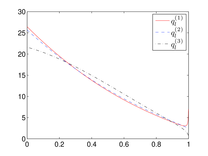
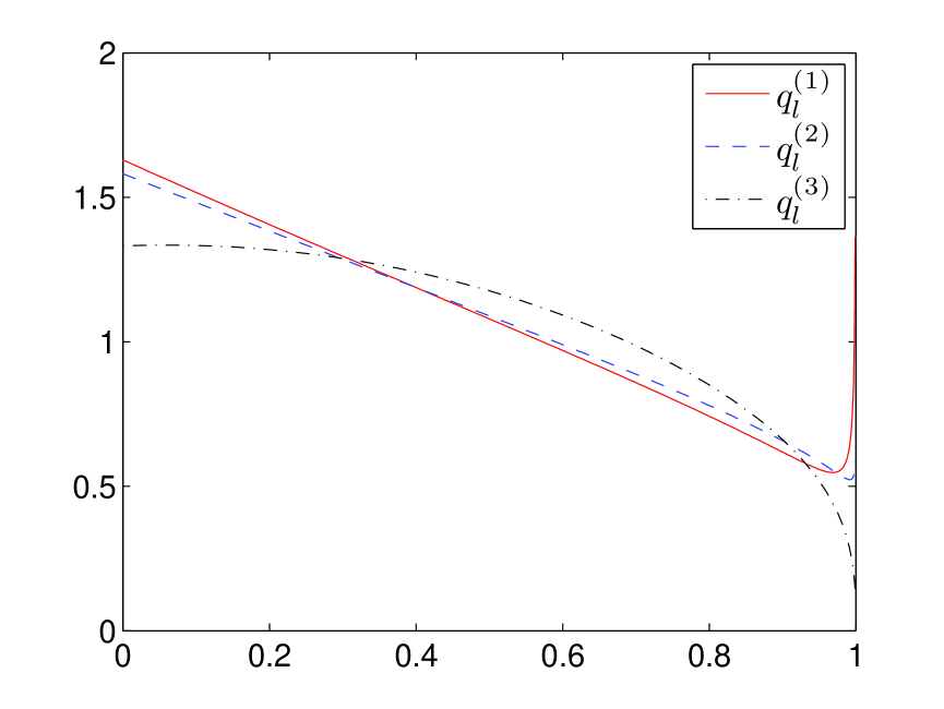
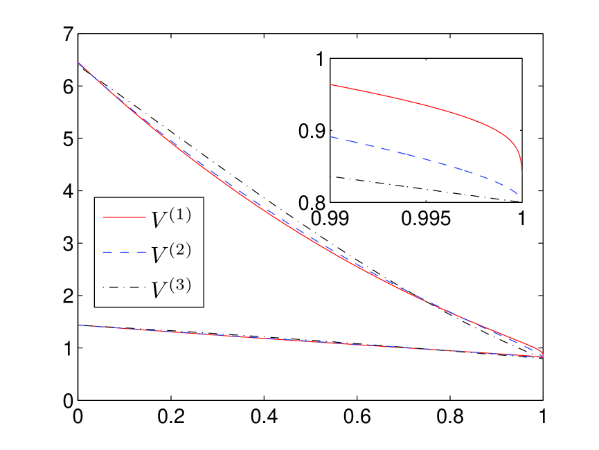
Figure 14: Distributions of the leak-off functions $q_{l}(t,x)$ and the respective particle velocity $V(t,x)$ over $\tilde{x}\in(0,1)$ at initial time $t=0$.

Note also, that by manipulating with the value of $\gamma$ one can simulate some very specific regimes of crack propagation. For example $\gamma=1/5$ corresponds to the constant injection flux rate, while $\gamma=1/3$ gives a constant crack propagation speed. For our computations we always set the value of $\gamma=1/5$.

Choosing appropriate values $b_{1}$ and $b_{2}$ one can change the relation between the amount of fluid loss to formation and the injection rate. This ratio can be defined by the measure, $Q_{l}/q_{0}$, where $Q_{l}$ is the total volume of leak-off $\int_{0}^{1}q_{l}dx$. It is important to note that this measure decreases in time, from its maximum value to zero, for all chosen benchmarks. Thus, taking the maximal value high enough and tracing the solution accuracy in time, one can analyse performance of the algorithm for any possible value of the parameter. We consider two variants of $Q_{l}/q_{0}$, one where fluid injection doubles the size of total fluid loss, and a second where the total fluid loss is close to injection rate. The values of the corresponding parameters $b_{1}$, $b_{2}$ are presented in Table 9.

	$Q_{l}/q_{0}=0.9$			$Q_{l}/q_{0}=0.5$
	$q_{l}^{(1)}$	$q_{l}^{(2)}$	$q_{l}^{(3)}$	$q_{l}^{(1)}$	$q_{l}^{(2)}$	$q_{l}^{(3)}$
$b_{1}$	$0.1$	$0.19$	$0.74$	$0.02$	$0.03$	$0.15$
$b_{2}$	$0.5$	$0.41$	$-0.13$	$0.1$	$0.08$	$-0.02$
$\gamma_{v}$	$1.69$	$1.70$	$1.65$	$0.55$	$0.56$	$0.55$

Table 9: The values of parameters $b_{1}$ and $b_{2}$ for different benchmark solutions modelling desired leak-off to fluid injection ratios.

Additionally one can compute a parameter $\gamma_{v}$ defined in Mishuris et al. (2012) as a measure of the uniformity of fluid velocity distribution:

$$\gamma_{v}=\left[\max(V(t,x))-\min(V(t,x))\right]\left[\int_{0}^{1}V(t,\xi)d\xi\right]^{-1}.$$ (95)

Interestingly, this measure is directly correlated with the leak-off ratio $Q_{l}/q_{0}$.

In Fig. 14 the distributions of the leak-off functions and the corresponding particle velocities for the respective benchmarks are presented. It shows that the velocity near the crack tip depends strongly on the benchmark variant. To highlight this fact, a zoom picture is placed in the Fig. 14 b).

Note that the benchmark $q_{l}^{(1)}$ is worse, in a sense, than the original Carter’s model as it contains additional singular terms of the leak-off function. These terms are absent in the normalised Carter’s law as it follows from Appendix B.

References

- Adachi and Detournay (2002) Adachi, J., Detournay, E. (2002) Self-similar solution of a plane-strain fracture driven by a power-law fluid. Int. J. Numer. Anal. Methods Geomech. 26, 579-604.
- Adachi and Peirce (2007) Adachi, JI., Peirce, AP. (2007) Asymptotic analysis of an elasticity equation for a finger-like hydraulic fracture. J. Elast. 90(1), 43-69.
- Adachi et al. (2007) Adachi, J., Siebrits E., Peirce A., Desroches J. (2007) Computer Simulation of Hydraulic Fractures. Int. J. Rock. Mech. Min. Sci., 44, 739-757.
- Aiken (1985) Aiken, RC. ed. (1985) Stiff Computation, Oxford University Press, Oxford.
- Carter (1957) Carter, E. (1957) Optimum fluid characteristics for fracture extension. In: Howard, G., Fast, C. (eds.) Drilling and Production Practices, 261-270. American Petroleum Institute.
- Crittendon (1959) Crittendon BC. (1959) The mechanics of design and interpertation of hydraulic fracture treatments. J. Pet. Tech., 21, 21-29.
- Clifton and Wang (1988) Clifton, RJ., Wang, JJ. (1988) Multiple fluids, proppant transport, and thermal effects in threedimensional simulation of hydraulic fracturing. SPE 18198.
- Desroches and Thiercelin (1993) Desroches J, Thiercelin M. (1993) Modeling the propagation and closure of micro-hydraulic fracturing. Int. J. Rock Mech. Min. Sci.; 30: 1231-4.
- Desroches et al. (1994) Desroches, J., Detournay, E., Lenoach, B., Papanastasiou, P., Pearson, J., Thiercelin, M., Cheng, A.-D. (1994) The crack tip region in hydraulic fracturing. Proc. Roy. Soc. Lond. Ser. A 447, 39-48.
- Detournay (2004) Detournay, E. 2004. Propagation regimes of fluid-driven fractures in impermeable rocks. Int J Geom 4, 1-11.
- Economides (2000) Economides, M., Nolte, K. (eds.). 2000. Reservoir Stimulation. 3rd edn. Wiley, Chichester, UK.
- Garagash et al. (2011) Garagash, D., Detournay, E., Adachi, J. (2011) Multiscale tip asymptotics in hydraulic fracture with leak-off. Journal of Fluid Mechanics, 669 260-297
- Geertsma and de Klerk (1969) Geertsma, J., de Klerk, F. (1969) A rapid method of predicting width and extent of hydraulically induced fractures. J Pet Tech, 21, 1571-1581 [SPE 2458]
- Harrison et al. (1954) Harrison, E., Kieschnick, WF., McGuire, WJ. (1954) The mechanics of fracture induction and extension. Petroleum Trans. AIME 201, 252-63
- Hubbert and Willis (1957) Hubbert, MK., Willis, DG. (1957) Mechanics of hydraulic fracturing. J. Pet. Tech. 9(6), 153-68.
- Khristianovic and Zheltov (1955) Khristianovic, SA., Zheltov, YP. (1955) Formation of vertical fractures by means of highly viscous liquid. In: Proceedings of the fourth world petroleum congress, Rome, 1955, 579-586.
- Kemp (1989) Kemp, LF. (1989) Study of Nordgren’s equation of hydraulic fracturing. SPE Production Eng. 5, 311-314.
- Kovalyshen and Detournay (2009) Kovalyshen, Y. and Detournay E. (2009) A Reexamination of the Classical PKN Model of Hydraulic Fracture, Transp Porous Med, 81, 317-339.
- Kovalyshen (2010) Kovalyshen, Y. (2010) Fluid-Driven Fracture in Poroelastic Medium. PhD Thesis, The University of Minnesota.
- Lenoach (1995) Lenoach, B., (1995) The crack tip solution for hydraulic fracturing in rock of arbitrary permeability Journal of the Mechanics and Physics of Solids, 43, 1025-1043
- Linkov (2011a) Linkov, AM. (2011) Speed Equation and Its Application for Solving Ill-Posed Problems of Hydraulic Fracturing. ISSM 1028-3358, Doklady Physics, 56(8), 436-438. Pleiades Publishing, Ltd. 2011
- Linkov (2011b) Linkov, AM. Use of a speed equation for numerical simulation of hydraulic fractures. arXiv:1108.6146, 2011
- Linkov (2011c) Linkov, AM. (2011) On numerical simulation of hydraulic fracturing. In: Proc. of XXXVIII summer school-conference ’Advanced Problems in Mechanics-2011’, Repino, St. Petersburg, July 1-5, 291-296.
- Linkov (2011d) Linkov, AM. (2011) On efficient simulation of hydraulic fracturing in terms of particle velocity. Int. J. Engng Sci, 52, 77-88.
- Lister (1990) Lister, JR. 1990, Buoyancy-driven fluid fracture: the effects of material toughness and of low-viscosity precursors. J Fluid Mech 210, 263-80.
- Mack and Warpinski (2000) Mack, MG., Warpinski, NR. (2000) Mechanics of hydraulic fracturing. In: Ecomides, Nolte, editors. Reservoire stimulation. 3rd ed. Chicester; Wiley: [Chapter 6]
- Mathias et al. (2009) Mathias, SA., van Reeuwijk, M. (2009) Hydraulic Fracture Propagation with 3-D Leak-off. Transport in Porous Media, 80, 499-518.
- Mishuris et al. (2012) Mishuris, G., Wrobel, M., Linkov A. (2012) On modeling hydraulic fracture in proper variables: stiffness, accuracy, sensitivity. Int. J. Engng Sci, 61, 10-23, December, 2012.
- Mitchell et al. (2007) Mitchell, SL., Kuske, R. and Peirce, A.P. (2007) An asymptotic framework for finite hydraulic fractures including leak-off, SIAM J. on Appl. Math., 67(2), 364-386
- Moschovidis et al. (2000) Moschovidis, ZA. and Steiger, RP. (2000) The Mounds drill-cuttings injection experiment:final results and conclusions. Proceedings of the IADC/SPE drilling conference, New Orleans,February 23-25. Richardson: Society of Petroleum Engineers;[SPE 59115]
- Nordgren (1972) Nordgren, RP. (1972) Propagation of a Vertical Hydraulic Fracture. J. Pet. Tech, 253, 306-314.
- Perkins and Kern (1961) Perkins, TK., Kern, LR. (1961) Widths of hydraulic fractures. J Pet Tech, 13(9): 37-49 [SPE 89]
- Pine and Cundall (1985) Pine, RJ., Cundall, PA. (1985) Applications of the Fluid-Rock Interaction Program (FRIP) to the modelling of hot dry rock geothermal energy systems. In: Proceedings of the international symposium on fundamentals of rock joints, Bjorkliden, Sweden, September 1985, 293-302.
- Rubin (1995) Rubin, AM. (1995) Propagation of magma filled cracks. Ann Rev Earth Planet Sci, 23, 287-336.
- Savitski and Detournay (2002) Savitski, A. and Detournay, E. (2002). Propagation of a fluid-driven penny-shaped fracture in an impermeable rock: Asymptotic solutions. Int. J. Solids Structures, 39(26):6311 6337.
- Sneddon and Elliot (1946) Sneddon, IN., Elliot, HA. (1946) The opening of a Griffith crack under internal pressure. Q Appl Math, 4, 262-267.
- Sneddon (1946) Sneddon, IN. (1946) The distribution of stress in the neighbourhood of a crack in an elastic solid. Proc R Soc London A, 187, 229-260.
- Spence and Sharp (1985) Spence, DA., Sharp, P. (1985) Self-Similar Solutions for Elastohydrodynamic Cavity Flow, Proc. R. Soc. Lond. A, 400, 289-313.
- Tsai and Rice (2010) Tsai, VC., Rice JR. (2010) A Model for Turbulent Hydraulic Hydraulic Fracture and Application to Crack Propagation at Glacier Beds, J. Geophys. Res., 115, 1-18.
- Wrobel and Mishuris (2013) Wrobel, M., Mishuris, G. (2013) Efficient pseudo-spectral solvers for the PKN model of hydrofracturing. International Journal of Fracture, April 2013, DOI 10.1007/s10704-013-9847-y