Magnetic field controlled vacuum charge in graphene quantum dots with a mass gap

Abstract

The effect of a magnetic field on the charged vacuum is investigated. The field dependence of the energy levels causes jumps in the total vacuum charge that occur whenever an energy level crosses the Fermi level and this leads to re-entrant cycles of vacuum charging and discharging. In atomic systems these effects require astrophysical magnetic fields of around $10^{8}$ T but in graphene with a mass gap they occur in laboratory fields of about 1 T or lower. It is suggested that an electrostatic graphene quantum dot defined by a gate electrode provides a solid state model of the as yet unobserved charged vacuum as well as a model of an atomic system in an extreme astrophysical environment. Phase diagrams are computed to show how the total vacuum charge depends on the confining potential strength and applied magnetic field. In addition the field dependence of the vacuum charge density is investigated and experimental consequences are discussed.

The long-sought-for charged vacuum PieperGershtein69 ; Greiner85 is the ground state of strong field quantum electrodynamics (QED). Usually the vacuum is neutral but it charges in the presence of an electric field strong enough to lower a bound state into the negative energy continuum. For example, when the charge on the nucleus of a hydrogenic atom increases to beyond $\sim 172$ the 1s state enters the negative energy continuum and if this happens at constant Fermi level, the vacuum charges. This is accompanied by spontaneous emission of two positrons which would enable the effect to be observed if a strong enough field could be created. In principle, this is possible because the critical charge can be exceeded in a collision between two uranium nuclei. But the interaction time is too short to allow the transition to a charged vacuum to occur Ruffini10 and, despite much effort, vacuum charging has not yet been observed. However, it may be possible to observe it in a semiconductor analogue.

The band gap of a semiconductor is analogous to the mass gap of an atomic system and semiconductor quantum dots are analogous to natural atoms qd . In electrostatic quantum dots, electrons are confined by an electrostatic potential that is generated by a gate electrode and replaces the Coulomb potential of a natural atom. Normally the dot is engineered so that the confined electron energies are just below the edge of the conduction band. But in a material with a small band gap it should be possible to use a stronger potential to lower a state into the valence band and create a charged vacuum analogue.

Any material that allows a state to be lowered into the valence band with a modest gate voltage is suitable. One candidate is monolayer graphene on substrates that induce a gap, for example BN bn , Ru Enderlein10 and controversially SiC sic . Other candidates include semiconducting carbon nanotubes and narrow gap semiconductors. Graphene is the only candidate with a Dirac-like energy dispersion and hence the candidate that provides the most precise analogue of QED. Indeed it has already been suggested that a charged vacuum occurs in graphene in the presence of a Coulomb impurity with enough charge Pereira08 but it is difficult to vary the impurity charge experimentally. However any attractive potential of sufficient strength charges the vacuum. This means a graphene quantum dot is an accurate and practical analogue of the atomic charged vacuum. In addition, dots made of materials with non-relativistic energy dispersion may allow studies of unusual charged vacua whose properties differ from the atomic one.

But the most interesting feature of the quantum dot analogue is that the charged vacuum is extremely sensitive to an external magnetic field. A rough estimate of the field needed to cause significant effects may be obtained by equating the rest mass-energy to the cyclotron energy. For atomic electrons this gives about $10^{10}$ T, an ultra strong magnetic field that only occurs in extreme astrophysical environments such as magnetized neutron stars Lai01 . In contrast, for graphene with $m_{0}c^{2}\sim 100$ meV and $c\sim 10^{6}$ ms^-1 the same estimate gives about 10 T, well inside the laboratory regime.

Moreover, important effects already occur at lower fields. Depending on their quantum numbers, energy levels both rise and fall as the magnetic field increases. If the energy of a charge carrying state rises above the Fermi level, the vacuum discharges while it charges if the energy of a state falls below the Fermi level. This leads to re-entrant cycles of vacuum charging and discharging. The relevant energy scale for these processes is the depth of the state in the continuum. For a hydrogenic atom with $Z=172$ this is about 15 keV Greiner85 and the field needed to discharge the vacuum is about $10^{8}$ T, still in the astrophysical regime, while for a graphene quantum dot it is $\lesssim 1$ T. These processes do not seem to have been investigated before and are studied here in the context of a graphene quantum dot. But the wave equation for a graphene dot is just the Dirac equation so exactly the same physics should occur in atomic systems in ultra strong magnetic fields. The graphene dot is not only an analogue of the charged vacuum but also an analogue of atomic physics in extreme astrophysical environments.

The objectives of this Letter are, first to demonstrate that charged vacuum states occur in graphene quantum dots, secondly to demonstrate magnetic field induced vacuum charging and discharging and finally to consider the experimental consequences. The dot is taken to be circularly symmetric and the electrostatic potential is modelled by $V(r)=V_{0}\exp(-(r/\lambda)^{p}/2)$ where $r$ is the radial co-ordinate, $|V_{0}|$ is the well depth and $\lambda=50$ nm is its width. $p$ determines the shape and slope of the well; the bottom flattens and the edge sharpens has $p$ increases (Fig. 1, top left). The magnetic field, $B$, is taken to be uniform and perpendicular to the dot plane and the quantum states are found by solving the two dimensional effective mass equation. Interestingly, the reduced spatial dimensions may make it easier to realise a charged vacuum Katsura06 . The mass is generated by including a site-dependent splitting parameter in the Hamiltonian, the same approach as in earlier work on graphene with a mass gap Pereira08 ; Giavaras11 .

The effective mass Hamiltonian for graphene consists of two $2\times 2$ blocks which together are equivalent to the 4-component Dirac Hamiltonian. One block gives the states near the $K$ point of the Brillouin zone and the other gives the states near $K^{\prime}$. The states near $K$ are obtained from the 2-component Hamiltonian $H=(\gamma/\hbar)\bm{\sigma}\cdot(\mathbf{p}+e\mathbf{A})+V+m_{0}c^{2}\sigma_{z},$ where the $\bm{\sigma}$ are Pauli matrices, $\mathbf{p}$ is the momentum and $\mathbf{A}$ is the magnetic vector potential. Here $c=\gamma/\hbar$, $\gamma$ is taken to be 646 meV nm Saito98 and $m_{0}c^{2}$ is taken to be 100 meV, the upper end of the observed range (10 - 100 meV). The eigenstates of a circularly symmetric dot are $\phi(\mathbf{r})=(\chi_{1}(r)\exp(i(m-1)\theta),\chi_{2}(r)\exp(im\theta))$, where $\theta$ is the azimuthal angle and $m$ is the total angular momentum quantum number. Equations for the radial functions are obtained by making the substitutions $f_{1}=\sqrt{r}\chi_{1}$, $if_{2}=\sqrt{r}\chi_{2}$. This leads to

$$\frac{V+m_{0}c^{2}}{\gamma}f_{1}+\left(\frac{d}{dr}+\frac{m-\frac{1}{2}}{r}+\frac{e}{\hbar}A_{\theta}\right)f_{2} = \frac{E}{\gamma}f_{1},$$

$$\left(-\frac{d}{dr}+\frac{m-\frac{1}{2}}{r}+\frac{e}{\hbar}A_{\theta}\right)f_{1}+\frac{V-m_{0}c^{2}}{\gamma}f_{2} = \frac{E}{\gamma}f_{2}.$$

These equations are discretized with a second order forward-backward difference scheme Giavaras12 which leads to a real, symmetric eigenvalue problem that is solved numerically. The states near $K^{\prime}$ are found in a similar way. The numerical system radius is 600 nm.

Physically, the valley index is equivalent to a pseudo-spin and the states near $K$ and $K^{\prime}$ correspond to pseudo-spin up and down respectively. The total angular momentum $\hbar(m-1/2)$ is the sum of the orbital angular momentum and pseudo-spin. The orbital angular momentum quantum number $l$ is therefore $m-1$ for states near $K$ and $m$ for states near $K^{\prime}$.

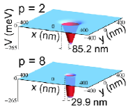
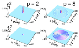
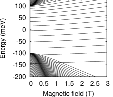
Figure 1: Model potentials (top left); well depth and field dependent energy levels (bottom) and typical states at $0.704$ T (top right).

Figure 1 shows the typical behaviour of energy levels and quantum states. The lower left frame shows the $K$ energy levels as a function of well depth when $B=0$, $m=1$ (i.e. $l=0$) and $p=2$. The results clearly show bound state levels plunging into the negative energy continuum as the well depth increases and similar behaviour is found for other values $m$ and $p$. The lower right frame shows the $K$ energy levels as a function of $B$ for the same parameters as in the lower left frame and well depth $265$ meV. The energy levels in the negative energy continuum continuum move down as $B$ increases but those of the bound states that have entered the continuum move up. The bound state level closest to the continuum edge crosses $E=-m_{0}c^{2}$ (dashed line) when $B\sim 2.4$ T and this corresponds to vacuum discharge in a system with Fermi level, $E_{F}\sim-m_{0}c^{2}$. The top right frame shows typical states. When a bound state enters the continuum it hybridizes with the continuum states and forms a Fano resonance Fano61 . Individual states that contribute to the resonance closest to the continuum edge are shown in the figure. The resonance width depends on the strength of the hybridization. Semi-classical analysis Maksym12a shows that a forbidden region surrounds the dot. As shown by the arrows in Fig. 1, the width of this forbidden region decreases when $p=8$ and this strengthens the hybridization Supplement . When $p=2$, the resonance width is less than the numerical continuum level separation ($\sim 1$ meV) and the resonance consists of one state. But when $p=8$, it involves about 2-4 states. In the case of Fig. 1, $B$ is chosen so that $f_{1}$ has the roughly the same amplitude for the 2 main contributing states and the resonance width is about 3 to 4 meV. The superposition of bound and continuum character is clearly visible. In contrast, strongly hybridized states do not normally occur in Coulomb potentials because the width of the forbidden region is large.

The vacuum charge density is the charge density induced in response to an external potential, $V$. It may be found from the commutator QED charge operator, $(-e/2)[\bar{\psi},\gamma^{0}\psi]$, where $\gamma^{0}$ is a Dirac matrix, $\psi$ is the Dirac field operator and $\bar{\psi}$ is its adjoint. Or it may be found from the normally ordered QED charge operator, $\hat{N}(-e\bar{\psi}\gamma^{0}\psi)$. Alternatively it is given by the standard form $\rho(V)-\rho(0)$ where $\rho$ is found by summing over states below $E_{F}$. The two QED operators are identical Bjorken65 . Further, both are equivalent to the standard form and this follows from their expectation values. The vacuum expectation value of the commutator operator is $\hat{\rho}(\mathbf{r})=(-e/2)(\sum_{E_{n}<E_{F},\alpha}|\phi_{n\alpha}(\mathbf{r})|^{2}-\sum_{E_{n}>E_{F},\alpha}|\phi_{n\alpha}(\mathbf{r})|^{2})$, where $\alpha$ represents the component and valley indices. The standard form is $-e\sum_{E_{n}<E_{F},\alpha}|\phi_{n\alpha}(\mathbf{r})|^{2}-\rho(0)=(-e/2)(\sum_{E_{n}<E_{F},\alpha}|\phi_{n\alpha}(\mathbf{r})|^{2}-\sum_{E_{n}>E_{F},\alpha}|\phi_{n\alpha}(\mathbf{r})|^{2})+[(-e/2)(\sum_{E_{n}<E_{F},\alpha}|\phi_{n\alpha}(\mathbf{r})|^{2}+\sum_{E_{n}>E_{F},\alpha}|\phi_{n\alpha}(\mathbf{r})|^{2})-\rho(0)])$. The terms in the square brackets vanish because of completeness and chiral symmetry Maksym12b so the standard form is equivalent to the QED forms. $\hat{\rho}$ is used to find the charge density and its integral gives the total vacuum charge $\hat{Q}=(-e/2)(\sum_{E_{n}<E_{F},\alpha}-\sum_{E_{n}>E_{F},\alpha})$. In QED the sums in $\hat{\rho}$ and $\hat{Q}$ are divergent and have to be treated with charge renormalization but they are convergent in the present numerical model because the energy spectrum is bounded.

Figure 2: Total vacuum charge as a function of well depth (left) and magnetic field (right).

The total vacuum charge as a function of well depth and magnetic field is shown in Fig. 2. Real spin splitting is included and the effective $g$-factor is taken to be 2.0. $E_{F}$ is just above $-m_{0}c^{2}$ so all real-spin-split Landau levels remain below it. For $B=0$ the vacuum charge increases monotonically with well depth in a series of steps. The first step occurs when the $l=0$ level shown in Fig. 1 enters the vacuum. Each step has height 4 and this corresponds to a 2-fold pseudo-spin degeneracy and a 2-fold real spin degeneracy. At constant well depth the vacuum charge as a function of $B$ shows re-entrant behaviour for both values of $p$. For instance, for well depth $220$ meV and $p=2$, it falls when $B\sim 0.41$ T and then rises when $B\sim 3.9$ T. The fall occurs because the $l=0$, $K$ level enters the continuum while the rise occurs because the $l=-1$, $K^{\prime}$ level leaves the continuum. The behaviour at larger well depth is similar but richer because some levels go through a minimum as a function of $B$ Maksym12b . Another effect of the field is real spin splitting. This allows an odd numbered vacuum charge and leads to double steps of height 1, for example at $B\sim 3.9$ T with well depth $220$ meV and $p=2$.

Figure 3: Vacuum charge phase diagrams for $p=2$ (left) and $p=8$ (right). $K$ phase boundaries solid, $K^{\prime}$ dashed.

To investigate the details, vacuum charge phase diagrams are computed (Fig. 3). Each phase boundary indicates where an energy level, $E_{n}$ crosses the Fermi level and is given implicitly by $E_{n}(V_{0},B)=E_{F}$. The total vacuum charge is shown on selected portions of the diagrams. For clarity real spin splitting is not included. Hence each line corresponds to a vacuum charge step of 2 electrons when $B\neq 0$ and 4 when $B=0$. The results in Fig. 2 are sections through the phase diagrams with real spin splitting included. The phase boundaries reflect the physics of the system: they have have small splittings at $B=0$, unless $l=0$, and there is pronounced $B$-dependent splitting. These effects can be understood from the non-relativistic limit of the effective mass equation. To order $1/m_{0}^{2}$ the splitting at $B=0$ results from the pseudo-spin-orbit interaction and the $B$-dependent splitting results from the interaction of the pseudo-spin with the magnetic field. Quantitatively, the exact splittings at $B=0$, $V_{0}=-180$ meV and $p=2$ are 1.05, 1.88 and 2.49 meV for the lowest states at $l=1$, 2, 3 respectively, while the lowest order pseudo-spin-orbit splittings are 1.36, 2.57 and 3.63 meV. The $B$-dependent splitting at 1 T, calculated from the pseudo-spin $g$-factor is 6.33 meV while the exact splitting at $l=0$ is 6.05 meV. Hence the non-relativistic limit describes the physics qualitatively but the exact equation is needed to find the splittings accurately.

Figure 4: Comparison of vacuum charge density and over and undercritical state densities (left); magnetic field dependence of $p=2$ vacuum charge density for 4 and 8 electrons (right).

Vacuum charge densities are shown in Fig. 4. The charge density increase associated with the charging steps is found from $\hat{\rho}(V_{0}+\delta V_{0})-\hat{\rho}(V_{0})$ where $\delta V_{0}$ is small ($-0.1$ meV). States below the threshold for vacuum charging are described as undercritical while those above it are called overcritical Greiner85 . The left side of the figure shows the charge density associated with the first step at $B=0$ T in Fig. 2. To a good approximation, the vacuum charge is stored in one overcritical state when $p=2$ and two when $p=8$. The open circles indicate the charge density computed from these few states. Near the peak they agree with the exact data to better than a few parts in 1000. The exact density is also well approximated by the undercritical bound state density (crosses). The $i$th overcritical state may be approximated Greiner85 by $a_{ib}\psi_{b}+\sum_{c}b_{ic}\psi_{c}$, where $\psi_{b}$ is the undercritical bound state and $\psi_{c}$ are undercritical negative continuum states. The coefficients $a_{ib}$ and $b_{ic}$ form a unitary transformation Greiner85 hence the approximate vacuum charge density reduces to $|\psi_{b}|^{2}$. The numerical data shows this approximation is accurate to a few parts in 1000 near the peak. A consequence of this approximate sum rule is that the vacuum charge density is hardly affected by hybridization with continuum states, although individual states contributing to it are.

The right hand frames of Fig. 4 illustrate the effect of the magnetic field on the vacuum charge density when $p=2$ and the total charge is 4 and 8 electrons. A magnetic field normally compresses the charge density because the cyclotron length is proportional to $1/\sqrt{B}$. However, in the present case the density expands because states of higher orbital angular momentum enter the vacuum when the $B$ increases. These states have a larger spatial extent so the density expands. For example, with 4 electrons at 0 T the charge density is composed of the 4-fold degenerate $l=0$ state while at 5 T it is composed of real and pseudo spin split states with $l=0$ and $l=-1$. The expansion continues until all the higher angular momentum states are exhausted.

There are several experimental consequences of these findings. First, the vacuum charge in a graphene quantum dot may be detectable via emssion of holes that is analogous to spontaneous positron emission. It may be possible to pump the gate voltage to enhance this effect. Secondly, the strong hybridization may be detectable with scanning tunnelling spectroscopy (STS). Although the hybridization does not affect the density, the states in Fig. 1 extend to a radius about an order of magnitude larger than the dot radius. They should be detectable when the experimental resolution is less than the width of the Fano resonance and this requires temperatures of a few K. Thirdly, it may be possible to detect the vacuum charge directly for example by capacitance measurements or quantum point contact electrometers. The ideal material for these experiments should be undoped or p-doped to ensure that an empty state is taken through the gap and it should be graphene with a gap to ensure that the effective mass equation is a precise analogue of the Dirac equation. Existing results bn ; Enderlein10 suggest that a suitable material can be found. In addition it should be possible to observe a charged vacuum analogue in narrow gap semiconductors or semiconducting carbon nanotubes, although the effective mass equation is no longer relativistic.

In summary, a quantum dot in graphene with a mass gap provides an accurate model of the charged vacuum. The vacuum charge is strongly affected by a magnetic field and a sufficiently high magnetic field can discharge the vacuum. These effects should also occur for atomic electrons in magnetic field but the small rest mass-energy of graphene charge carriers, allows them to be seen with fields $\sim 1$ T instead of the extreme astrophysical fields needed for atomic electrons. Experimentally, it may be possible to detect the graphene charged vacuum directly, or by observation of hole emission or by probing the states with STS. The effect of interactions remains to be investigated but a Thomas-Fermi approach Greiner85 suggests the atomic vacuum charge survives the effect of interactions.

We thank Seigo Tarucha, Michihisa Yamamoto and Robin Nicholas for useful discussions. This work was supported by the UK Royal Society and the Japanese ministry of education, Scientific Research No. 23340112.

References

- (1) S. Gershtein and Y. B. Zeldovich, Lett. Nuovo Cimento 1, 835 (1969); W. Pieper and W. Greiner, Z. Phys. 218 327 (1969).
- (2) W. Greiner, B. Müller and J. Rafelski, Quantum Electrodynamics of Strong Fields, Springer, New York (1985).
- (3) R. Ruffini, G. Vereshchagin and She-Sheng Xue, Phys. Repts. 487, 1 (2010).
- (4) P. A. Maksym, H. Imamura, G. P. Mallon and H. Aoki, J. Phys. Condens. Mat. 12, R299 (2000); L. P. Kouwenhoven, D. G. Austing and S. Tarucha, Repts. Prog. Phys. 64, 701 (2001); G. Giavaras, P. A. Maksym and M. Roy, J. Phys: Condens. Mat. 21, 102201 (2009); P. A. Maksym, M. Roy, M. F. Craciun, M. Yamamoto, S. Tarucha and H. Aoki, J. Phys.: Conf. Ser. 245 012030 (2010).
- (5) G. Giovannetti, P. A. Khomyakov, G. Brocks, P. J. Kelly and J. van den Brink, Phys. Rev. B 76, 073103 (2007); L. Ci, L. Song, C. Jin, D. Jariwala, D. Wu, Y. Li, A. Srivastava, Z. F. Wang, K. Storr, L. Balicas, F. Liu, and P. M. Ajayan, Nat. Mater. 9, 430 (2010); C. Yelgel and G. P. Srivastava, Appl. Surf. Sci. 258, 8342 (2012).
- (6) C. Enderlein, Y. S. Kim, A. Bostwick, E. Rotenberg and K. Horn, New J. Phys. 12, 033014 (2010).
- (7) S. Y. Zhou, G.-H. Gweon, A. V. Fedorov, P. N. First, W. A. de Heer, D.-H. Lee, F. Guinea, A. H. Castro Neto and A. Lanzara, Nat. Mater. 6, 770 (2007); L. Vitali, C. Riedl, R. Ohmann, I. Brihuega, U. Starke and K. Kern Surf. Sci. 602, L127 (2008); A. Bostwick, T. Ohta, J. L. McChesney, K. V. Emtsev, T. Seyller, K. Horn and E. Rotenberg, New J. Phys. 9 385 (2007); W. A. de Heer, C. Berger, X. Wu, M. Sprinkle, Y. Hu, M. Ruan, J. A. Stroscio, P. N. First, R. Haddon, B. Piot, C. Faugeras, M. Potemski and J-S Moon, J. Phys. D: Appl. Phys. 43 374007 (2010).
- (8) V. M. Pereira, V. N. Kotov and A. H. Castro Neto, Phys. Rev. B 78, 085101 (2008).
- (9) D. Lai, Rev. Mod. Phys. 73, 629 (2001).
- (10) H. Katsura and H. Aoki, J. Math. Phys. 47, 032301 (2006).
- (11) G. Giavaras and Franco Nori, Phys. Rev. B 83, 165427 (2011).
- (12) R. Saito, G. Dresselhaus and M. S. Dresselhaus, Physical Properties of Carbon Nanotubes, Imperial College Press, London (1998).
- (13) G. Giavaras, P. A. Maksym and M. Roy, in preparation.
- (14) In the magnetic field range considered the levels are very close to each other and are referred to as a continuum.
- (15) U. Fano, Phys. Rev. 124, 1866 (1961).
- (16) P. A. Maksym and G. Giavaras, in preparation.
- (17) See supplemental material.
- (18) J. D. Bjorken and S. D. Drell, Relativistic Quantum Fields, McGraw-Hill, New York (1965).
- (19) P. A. Maksym and H. Aoki, submitted to Proc. HMF20.