On the Minimal Scattering Response of PEC Cylinders in a Dielectric Cloak

Abstract

Recently, it was shown that an infinite perfectly conducting (PEC) cylinder can be nearly perfectly cloaked from normally incident electromagnetic waves using a single-layer homogeneous dielectric cladding. Here we study the electromagnetic response of such structures with the goal to understand the main mechanisms underpinning this cloaking phenomenon. We introduce a simple model of the cloaked PEC cylinder, replacing it by an omnidirectional electric-line scatterer and a bipolar magnetic one; accordingly, the far field is determined in a compact closed form. The analysis of the results shows that the optimal cloaking regime corresponds to the frequency point where the total electric moment is drastically mitigated and thus the radiation pattern of the device resembles that of a magnetic-dipole line. In the vicinity of the optimal cloaking frequency we observe the response close to that of Huygens’ pairs of electric and magnetic line scatterers.

1 Introduction

Cloaking devices render objects partially or wholly invisible to parts of the electromagnetic spectrum by drastically reducing the total scattering cross section of the objects. Due to the obvious interest in potential applications and due to their intriguing nature, cloaks have attracted considerable attention from both practical experts and theoretical scientists during the previous decade. In the pioneering works [1, 2], the control of electromagnetic fields in order to not to interact with an object is theoretically formulated. They use optical conformal mapping techniques and complex coordinate transformations which require exotic inhomogeneous and anisotropic materials. On the other hand, actual structures realizing broadband electromagnetic cloaking with, e.g., transmission lines, are presented in the papers [3, 4], where experimental validation is provided. Furthermore, the so-called “scattering cancellation” technique has been introduced in [5], where drastic reduction of the scattering response of a specific dielectric object is accomplished with a dielectric covering layer.

In this paper we consider cloaking of infinite perfectly-conducting (PEC) cylinders using the simplest possible configuration: a uniform dielectric cover [6]. A PEC circular cylinder is covered by a single cladding and is excited by a plane wave (whose electric field is parallel to the cylinder axis), formulating a two-dimensional (2D) boundary-value problem. This geometric configuration is the same as that for scattering cancellation cloaking of dielectric cylinders [5], but the physical phenomena leading the the cloaking effect are different and the known design methods for scattering-cancellation cloaks cannot be used for this polarization [7]. In fact, the equations for the required thickness and material parameters of the cloaking cladding have no solution for the case of a PEC cylinder in the center [5, 7]. However, similar devices have been analyzed in electrostatic [8], in quasi-static [9] and in electrodynamic [6] regimes and satisfying cloaking performances have been achieved. It is therefore important to understand the phenomenon and develop a predictive analytical model, enabling the design of cloaks for elongated conductive objects.

Here we introduce an approximate model that can be used in explaining and interpreting the aforementioned interesting behavior. In particular, we note that the scattering pattern of cloaked PEC cylinders in the vicinity of the optimal cloaking frequency is similar to simple dipolar objects. In addition, we expect that the optimal cloaking regime should correspond either to minimization of induced lowest-order moment(s) or to the electric and magnetic moments forming a Huygens’ pair with the minimum scattering in the forward direction. This brings us to the idea to model the cylindrical volume by one electric and one magnetic dipole line located along the central axis. The corresponding moments are evaluated analytically from the canonical field solution and the scattered field of the equivalent structure is expressed in a compact form. After validating the model by comparing the data originating from the exact solution with that given by the approximate model, we discuss the frequency response of the equivalent system. Certain conclusions related to the principle of the device operation and justification of the cloaking phenomenon are drawn. Some preliminary results of this study have been reported in a conference [10].

2 Electromagnetic Fields

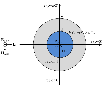
Figure 1: A simple 2D structure of a PEC cylinder of radius $g$ covered by a magnetically inert layer of thickness $(a-g)$ and relative permittivity $\epsilon_{r}$, is illuminated by a plane wave.

Let us consider a simple two-dimensional (2D) structure depicted in Fig. 1. An infinite PEC cylinder of the radius $g$ is covered by a single isotropic and uniform dielectric layer of the thickness $(a-g)$. The cladding layer (Region 1) is filled with a magnetically inert material of the relative permittivity $\epsilon_{r}$. The whole structure is placed in vacuum (Region 0, the permittivity $\epsilon_{0}$, and the permeability $\mu_{0}$). The axis of the cylinder coincides with the z axis of the cylindrical coordinate system $(\rho,\phi,z)$, which can be used interchangeably with the corresponding Cartesian one $(x,y,z)$. This cylindrical configuration is illuminated by a z-polarized (TE or TM_z in an alternative definition) plane wave of unitary electric-field magnitude propagating along the positive x semi-axis [11]:

$$\textbf{E}_{0,inc}=\textbf{z}E_{z0,inc}(\rho,\phi)=\textbf{z}\sum_{n=0}^{+\infty}A_{0}(n)J_{n}(k_{0}\rho)\cos(n\phi),$$ (1)

where $A_{0}(n)=\frac{2}{1+\delta_{n0}}j^{-n}$, $k_{0}=2\pi f\sqrt{\epsilon_{0}\mu_{0}}$ is the free-space wavenumber and $f$ is the operational frequency. The notation $J_{n}$ concerns the Bessel function of $n$-th order, while the symbol $\delta_{n0}$ corresponds to the Kronecker delta. The harmonic time dependence is of the form $e^{+j2\pi ft}$ and suppressed throughout the analysis.

Due to the 2D nature of the studied configuration and the isotropy of the materials, the (secondary) electric field in each of the two regions (0, 1) is z-polarized and can be expressed in the following forms:

$$E_{z0,scat}(\rho,\phi)=\sum_{n=0}^{+\infty}B_{0}(n)H_{n}^{(2)}(k_{0}\rho)\cos(n\phi),$$ (2)

$$E_{z1}(\rho,\phi)=\sum_{n=0}^{+\infty}\left[A_{1}(n)J_{n}(k\rho)+B_{1}(n)H_{n}^{(2)}(k\rho)\right]\cos(n\phi),$$ (3)

where $H_{n}^{(2)}=J_{n}-jY_{n}$ is the Hankel function of $n$-th order. The wavenumber in region 0 is defined as $k=k_{0}\sqrt{\epsilon_{r}}$.

By imposing the necessary boundary conditions around the cylindrical surfaces $\rho=g,a$, the unknown coefficient sequences $B_{0}(n),A_{1}(n),B_{1}(n)$ of (2), (3) are readily determined. The azimuthal magnetic component in region 1 is expressed as:

$$H_{\phi 1}(\rho,\phi)=-\frac{j}{k_{0}\zeta_{0}}k\sum_{n=0}^{+\infty}\left[A_{1}(n)J^{\prime}_{n}(k\rho)+B_{1}(n)H_{n}^{(2)\prime}(k\rho)\right]\cos(n\phi),$$ (4)

where $\zeta_{0}=\sqrt{\mu_{0}/\epsilon_{0}}=120\pi~{}\Omega$ is the wave impedance of vacuum. Based on these field quantities, the equivalent dipole moments can be rigorously evaluated. Furthermore, the far-field response of the cylindrical structure is determined with the use of Hankel’s expansion for large arguments: $H_{n}^{(2)}(k_{0}\rho)\sim\sqrt{\frac{2}{\pi k_{0}\rho}}e^{-j\left(k_{0}\rho-\frac{n\pi}{2}-\frac{\pi}{4}\right)},k_{0}\rho\rightarrow+\infty$. In particular,

$$E_{z0,scat}(\rho,\phi)\sim\sqrt{\frac{2}{\pi k_{0}\rho}}e^{-j(k_{0}\rho-\frac{\pi}{4})}\sum_{n=0}^{+\infty}B_{0}(n)j^{n}\cos(n\phi),\quad k_{0}\rho\rightarrow+\infty.$$ (5)

3 Electromagnetic Moments

3.1 Equivalent Current

The surface current induced at the PEC surface $\rho=g$ is given by:

$$\textbf{K}(\phi)=\textbf{z}H_{\phi 1}(g,\phi).$$ (6)

By definition, the polarization current over the cross sections of the cladding layer is written as follows:

$$\textbf{J}_{pol}(\rho,\phi)=\textbf{z}j\frac{k_{0}}{\zeta_{0}}(\epsilon_{r}-1)E_{z1}(\rho,\phi).$$ (7)

Consequently, the total induced current which is the source of the scattering field by the cylindrical structure possesses the form:

$$\textbf{J}(\rho,\phi)=\textbf{K}(\phi)\delta(\rho-g)+\textbf{J}_{pol}(\rho,\phi)$$

$$=\textbf{z}H_{\phi 1}(g,\phi)\delta(\rho-g)+\textbf{z}j\frac{k_{0}}{\zeta_{0}}(\epsilon_{r}-1)E_{z1}(\rho,\phi),$$ (8)

where $\delta$ is the Dirac function.

3.2 Electric Moment

The electric moment p of electric current density J existing in a volume $(V)$ is defined in [12] and can be written in the 2D case as an integral over the cross-section surface $(S)$:

$$\textbf{p}=\frac{1}{j2\pi f}\iiint_{(V)}\textbf{J}~{}dV\Rightarrow\textbf{p}^{*}=\frac{1}{j2\pi f}\iint_{(S)}\textbf{J}~{}dS,$$ (9)

where $\textbf{p}^{*}$ is the electric moment per unit length (p.u.l.) of the z axis. If one substitutes expression (8) into formula (9), only the 0-th term from the harmonic series (3), (4) survives; accordingly, the following expression is obtained:

$$\textbf{p}^{*}=\textbf{z}\frac{2\pi}{k_{0}^{2}\zeta_{0}c}\left\{\begin{array}[]{c}k_{0}^{2}(\epsilon_{r}-1)\left[A_{1}(0)V_{J}(g,a,k)+B_{1}(0)V_{H}(g,a,k)\right]\\ -kg\left[A_{1}(0)J^{\prime}_{0}(kg)+B_{1}(0)H_{0}^{(2)\prime}(kg)\right]\end{array}\right\},$$ (12)

where $c=\frac{1}{\sqrt{\epsilon_{0}\mu_{0}}}$ is the speed of light. The integrals of the Bessel and Hankel functions are analytically evaluated:

$$V_{J}(\chi,\psi,k)=\int_{\chi}^{\psi}J_{0}(k\rho)\rho d\rho=\frac{\psi J_{1}(k\psi)-\chi J_{1}(k\chi)}{k},$$ (13)

$$V_{H}(\chi,\psi,k)=\int_{\chi}^{\psi}H_{0}^{(2)}(k\rho)\rho d\rho=\frac{\psi H_{1}^{(2)}(k\psi)-\chi H_{1}^{(2)}(k\chi)}{k}.$$ (14)

This quantity $\textbf{p}^{*}=\textbf{z}~{}p_{z}^{*}$ (in Coulomb) expresses mainly how powerful is the total induced electric current for given device dimensions and the frequency. It can be considered as a 2D electric dipole line (or an electric current line) along the central axis of the structure, which models the electric response of the whole cylindrical configuration.

3.3 Magnetic Moment

The magnetic moment m of a volumetric distribution of electric current density J existing in volume $(V)$ is defined in [13] and can be rewritten in the 2D case as a surface integral over the cross section $(S)$:

$$\textbf{m}=\frac{1}{2}\iiint_{(V)}\textbf{r}\times\textbf{J}~{}dV\Rightarrow\textbf{m}^{*}=\frac{1}{2}\iint_{(S)}\textbf{r}\times\textbf{J}~{}dS,$$ (15)

where $\textbf{r}={\bm{\rho}}\rho+\textbf{z}z$ is the observation vector in cylindrical coordinates and $\textbf{m}^{*}$ is the magnetic moment per unit length (p.u.l.) of the z axis. Obviously, the vector $(\textbf{r}\times\textbf{J})$ has exclusively an azimuthal (${\bm{\phi}}$) component. Due to the orthogonality of the cylindrical functions, only the 1-st term from the harmonic series (3), (4) survives. Writing the unit vector along ${\bm{\phi}}$ in the Cartesian coordinates: ${\bm{\phi}}=-\textbf{x}\sin\phi+\textbf{y}\cos\phi$, we see that the vector of the magnetic dipole moment is parallel to the y axis (the term $\textbf{x}\sin\phi$ gives an odd function with zero contribution to the integral). Accordingly, one obtains the result:

$$\textbf{m}^{*}=-\textbf{y}\frac{j\pi}{2k_{0}\zeta_{0}}\left\{\begin{array}[]{c}k_{0}^{2}(\epsilon_{r}-1)\left[A_{1}(1)W_{J}(g,a,k)+B_{1}(1)W_{H}(g,a,k)\right]\\ -kg^{2}\left[A_{1}(1)J^{\prime}_{1}(kg)+B_{1}(1)H_{1}^{(2)\prime}(kg)\right]\end{array}\right\}.$$ (18)

Again, the related integrals of the Bessel and Hankel functions are rigorously determined as follows:

$$W_{J}(\chi,\psi,k)=\int_{\chi}^{\psi}J_{1}(k\rho)\rho^{2}d\rho=\frac{\psi^{2}J_{2}(k\psi)-\chi^{2}J_{2}(k\chi)}{k},$$ (19)

$$W_{H}(\chi,\psi,k)=\int_{\chi}^{\psi}H_{1}^{(2)}(k\rho)\rho^{2}d\rho=W_{J}(\chi,\psi,k)$$

$$-\frac{j}{2}\left\{\begin{array}[]{c}\psi^{3}M\left(\left[\begin{array}[]{c}-\frac{1}{2}\\ -1\end{array}\right],\left[\begin{array}[]{cc}-\frac{1}{2}&\frac{1}{2}\\ -\frac{3}{2}&-1\end{array}\right],\frac{k\psi}{2},\frac{1}{2}\right)\\ -\chi^{3}M\left(\left[\begin{array}[]{c}-\frac{1}{2}\\ -1\end{array}\right],\left[\begin{array}[]{cc}-\frac{1}{2}&\frac{1}{2}\\ -\frac{3}{2}&-1\end{array}\right],\frac{k\chi}{2},\frac{1}{2}\right)\end{array}\right\},$$ (30)

where $M$ is the Meijer function [14]. This quantity $\textbf{m}^{*}=\textbf{y}~{}m_{y}^{*}$ (in Ampere$\cdot$meter) expresses mainly how powerful is the spatial variation of the induced electric current over the cross section of the device for given device dimensions and the frequency. It is a 2D magnetic dipole line positioned along the central axis of the structure.

In the following we will see that this simple model adequately represents the response of the cloaked cylinder near the optimal operational frequency despite the fact that the variations of the fields inside the cloak are quite significant (its electrical size is considerable due to high permittivity of the cladding cylinder).

3.4 Radiation Fields

The radiated electric field $\textbf{E}_{p}$ by an electric moment $\textbf{p}^{*}$ p.u.l. of the axis z in a 2D configuration is written as follows [15]:

$$\textbf{E}_{p}(\rho,\phi)=\frac{1}{\epsilon_{0}}\nabla\times\left[\nabla G(\rho,\phi)\times\textbf{p}^{*}\right],$$ (31)

where $G$ is the scalar Green’s function in two dimensions, expressed in cylindrical coordinates. It corresponds to the field at a point $(\rho,\phi)$ developed from a singular source at $(P,\Phi)$. In our case, the position of this dipole coincides with the z axis $(P=0)$ of the coordinate system; therefore, the respective expression takes the form [16]:

$$G(\rho,\phi)=-\frac{j}{4}H_{0}^{(2)}(k_{0}\rho).$$ (32)

Similarly, the radiated electric field $\textbf{E}_{m}$ produced by a magnetic-moment line $\textbf{m}^{*}$ p.u.l. at the axis z in a 2D configuration is given by [15]:

$$\textbf{E}_{m}(\rho,\phi)=-j2\pi f\mu_{0}\nabla G(\rho,\phi)\times\textbf{m}^{*}.$$ (33)

If one takes into account the polarization of the moments $(\textbf{p}^{*}=\textbf{z}~{}p_{z}^{*},\textbf{m}^{*}=\textbf{y}~{}m_{y}^{*})$, substitutes Green’s function (32) and adds the two electric fields (31), (33), the total developed field $(\textbf{E}_{p}+\textbf{E}_{m})$ from the moments couple possesses a single z component given by:

$$E^{\prime}_{z0,scat}(\rho,\phi)=\frac{k_{0}^{2}\zeta_{0}}{4}\left[m_{y}^{*}H_{1}^{(2)}(k_{0}\rho)\cos\phi-jcp_{z}^{*}H_{0}^{(2)}(k_{0}\rho)\right].$$ (34)

The corresponding far-field expression reads:

$$E^{\prime}_{z0,scat}(\rho,\phi)\sim\sqrt{\frac{2}{\pi k_{0}\rho}}e^{-j(k_{0}\rho-\frac{\pi}{4})}\frac{k_{0}^{2}\zeta_{0}}{4j}\left[cp_{z}^{*}-m_{y}^{*}\cos\phi\right],\quad k_{0}\rho\rightarrow+\infty.$$ (35)

The two electric fields $E_{z0,scat}(\rho,\phi)$ and $E^{\prime}_{z0,scat}(\rho,\phi)$ represent the same physical quantity, namely the field scattered by the cylindrical structure under the plane wave excitation. The difference is that the first one (the unprimed, denoted by: $E_{z0,scat}(\rho,\phi)$) is evaluated from the explicit forms of the fields determined through the rigorous canonical solution of the scattering problem, while the second one (the primed, denoted by: $E^{\prime}_{z0,scat}(\rho,\phi)$) is computed from the approximate model of two scattering dipole lines.

4 Total Scattering Quantities

By repeating the same procedures described above, one can readily find the corresponding field quantities $\tilde{E}_{z0,scat}(\rho,\phi)$, $\tilde{E}^{\prime}_{z0,scat}(\rho,\phi)$ which describe the situation of a bare PEC cylinder of radius $g$ in the absence of the cladding (our solution for $\epsilon_{r}=1$). In this way, one can define the normalized total scattering widths in each case as follows:

$$\sigma_{norm}=\lim_{k_{0}\rho\rightarrow+\infty}\frac{\int_{0}^{2\pi}|E_{z0,scat}(\rho,\phi)|^{2}d\phi}{\int_{0}^{2\pi}|\tilde{E}_{z0,scat}(\rho,\phi)|^{2}d\phi},$$ (36)

$$\sigma^{\prime}_{norm}=\lim_{k_{0}\rho\rightarrow+\infty}\frac{\int_{0}^{2\pi}|E^{\prime}_{z0,scat}(\rho,\phi)|^{2}d\phi}{\int_{0}^{2\pi}|\tilde{E}^{\prime}_{z0,scat}(\rho,\phi)|^{2}d\phi}.$$ (37)

These quantities measure the reduction of total scattering from the PEC cylinder due to cloaking cladding (when $\sigma_{norm},\sigma^{\prime}_{norm}\rightarrow 0$, we have perfect cloaking effect). Also here $\sigma_{norm}$ and $\sigma^{\prime}_{norm}$ give the normalized scattering widths computed from the rigorous solution and the dipole moments, respectively.

The forward scattering theorem [17] is a well-known lemma, frequently used in electromagnetics, which relates the scattered field by a lossless object $E_{z0,scat}(\rho,\phi),E^{\prime}_{z0,scat}(\rho,\phi)$, along the forward direction (namely the one of the incident plane wave, here: $\phi=0$) with the total scattered power from the object. In particular, this power (expressed in Watt) is given by:

$$P_{scat}=-\frac{\sqrt{2}}{k_{0}\zeta_{0}}\Re\left[\sum_{n=0}^{+\infty}B_{0}(n)j^{n}\right],$$ (38)

$$P^{\prime}_{scat}=-\frac{k_{0}}{2\sqrt{2}}\Im\left[cp_{z}^{*}-m_{y}^{*}\right],$$ (39)

respectively to which method we adopt (the full-wave solution or the moments model). In other words, in the case of a perfect cloak, the electric quantity $\Im[cp_{z}^{*}]$ should be equal and opposite to the magnetic quantity $\Im[-m_{y}^{*}]$. The two sources $\Im[cp_{z}^{*}],\Im[-m_{y}^{*}]$ are cooperating with each other to produce mutually neutralized scattering.

5 Numerical Results

5.1 Parameters

Before proceeding with the discussion of the results, we need to define the value ranges of the problem parameters. As the reference operational frequency of the cloak, we assume $f_{0}=3\cdot 10^{8}$ Hz corresponding to unitary free-space wavelength $\lambda_{0}=1$ m. The physical size of the considered structure is kept constant throughout the numerical simulations to simplify the procedure and highlight the effect of variations of the other parameters. More specifically, we take $g=0.05\lambda_{0}$ and $a=0.08\lambda_{0}$. This assumption does not affect the generality of our investigation because similar dependencies are observed for other dimensions. Since the operational frequency does not differ significantly from $f_{0}$, the electrical dimension of the PEC cylinder is close to 10% of the free-space operational wavelength. In other words, cloaking (even not perfectly) this conducting volume is not a trivial task since its electrical size is far from infinitesimal even in terms of the free-space wavelength.

5.2 Graphs

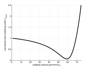
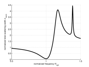
Figure 2: The normalized total scattering width $\sigma_{norm}$ as function of: (a) the cladding relative permittivity $\epsilon_{r}$ ($f=f_{0}$) and (b) the normalized operating frequency $f/f_{opt}$ ($\epsilon_{r}=60$). Plot parameters: $f_{0}=c/\lambda_{0}=3\cdot 10^{8}$ Hz, $f_{opt}=0.992f_{0}$, $g/\lambda_{0}=0.05$, $a/\lambda_{0}=0.08$.

In Fig. 2 we sweep the relative permittivity of the cladding $\epsilon_{r}$ and evaluate the normalized total scattering width using the exact field formulas. The operating frequency is kept constant $f=f_{0}$ and the optimal cloaking result (the minimum $\sigma_{norm}$) is obtained for $\epsilon_{r}\cong 60$. Therefore, the dielectric constant is kept fixed to this value hereinafter to emphasize the frequency response of the device. Needless to say that additional minima are recorded for higher frequencies, but we are interested in the cloaking regime at the lowest possible frequency (not so high permittivity and electrical size). In Fig. 2 we plot the same quantity $\sigma_{norm}$ with respect to the frequency. The optimal frequency $f_{opt}$ is very close to $f_{0}$ ($f_{opt}=0.992f_{0}$) but not exactly equal to that since the choice $\epsilon_{r}=60$ does not correspond to the optimal case of Fig. 2. Additionally, the shape of the two curves in Figs. 2 are similar since the horizontal axis corresponds to a common quantity: the effective electrical distance inside the cladding.

In Figs. 3, we “zoom” in the operation of the device close to the optimal frequency $f=f_{opt}$ to better understand the cloaking effect. In particular, we assemble five graphs of the normalized scattering patterns of the cylindrical structure, defined by $\lim_{k_{0}\rho\rightarrow+\infty}\frac{|E_{z0,scat}(\rho,\phi)|}{|\tilde{E}_{z0,scat}(\rho,\phi)|}$ for $f/f_{opt}=0.95,0.98,1,1.02,1.05$. We observe that the polar plots differ substantially from each other despite the smallness of variations of $f$. More specifically, a backward scattering for $f<f_{opt}$ and a forward scattering effect for $f>f_{opt}$ has been recorded. Exactly at $f=f_{opt}$, we obtain a bipolar plot which means that the first $(n=1)$ term in series (2), (5) becomes dominant in defining the scattering pattern. To put it alternatively, the omnidirectional zeroth term $(n=0)$ is suppressed at $f=f_{opt}$ and increases rapidly when going away from this point. Such behavior reminds us clearly of the scattering cancellation principle [5] which is reported as being not feasible for PEC cores and the considered TE (referred to as TM_z in [7]) polarization. Consequently, the present cloaking technique can be characterized as an “expanded scattering cancellation” suitable for cloaking of PEC cylinders. In fact, we have achieved a $de~{}facto$ scattering cancellation effect for PEC objects. Such a feature has been briefly referred in [19].

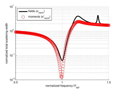
Figure 4: The normalized total scattering width as function of the normalized operating frequency $f/f_{opt}$ when evaluated through the exact field solution $(\sigma_{norm})$ and when computed from the approximate moments model $(\sigma^{\prime}_{norm})$. Plot parameters: $f_{0}=c/\lambda_{0}=3\cdot 10^{8}$ Hz, $f_{opt}=0.992f_{0}$, $g/\lambda_{0}=0.05$, $a/\lambda_{0}=0.08$, $\epsilon_{r}=60$.

To study the phenomena in the vicinity of the optimal cloaking frequency $f=f_{opt}$, we adopt the simplified analytical approach with the equivalent moments described in Section III. We represent the variation of the normalized total scattering width when computed with the exact field formulas ($\sigma_{norm}$) and when evaluated from the respective moments ($\sigma^{\prime}_{norm}$) in the same diagram (Fig. 4), as functions of the normalized frequency $f/f_{opt}$. The former graph is the same as Fig. 2, and the latter exhibits remarkable agreement with the first one, especially for smaller frequencies. In the vicinity of the cloaking regime, the model certainly “captures” the physics in terms of the minimized scattering; implicitly, optimal frequency $f^{\prime}_{opt}$ in the moments case is only slightly lower than $f_{opt}$ ($f^{\prime}_{opt}=0.984f_{0}$). However, the exact level of the maximum reduction cannot be predicted successfully since $\sigma^{\prime}_{norm}$ is much smaller than the actual $\sigma_{norm}$. This difference is due to the fact that the higher-order terms $(n>1)$ in (2), (5) are significant at $f\cong f_{opt},f^{\prime}_{opt}$ where the scattering due to the leading term is mitigated. Their effect is mutually canceled in the radiation pattern of Fig. 3 but they indeed substantially contribute to the overall scattered power and define this gap between the levels of $\sigma_{norm}$ and $\sigma^{\prime}_{norm}$ as shown in Fig. 4. Moreover, when the operational frequency gets higher, the moments model becomes inaccurate since it replaces the entire structure by a pair of dipoles. In other words, electrically thick cylinders, that imply strong azimuthal variations of induced polarization, cannot be fitted with the few degrees of freedom of our approximate moments model. However, the model results exhibit satisfying similarity with the actual field waveforms at the moderate frequencies and imitate successfully the developed physical mechanism at the cloaking regime.

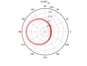
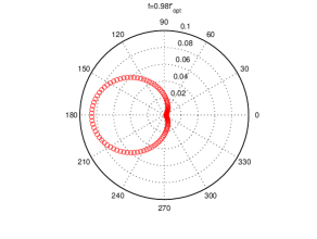
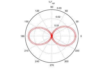
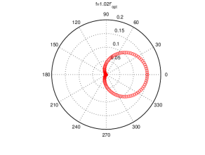
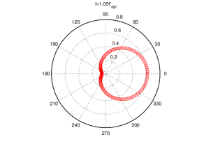
Figure 5: The normalized radiation patterns $\lim_{k_{0}\rho\rightarrow+\infty}\frac{|E^{\prime}_{z0,scat}(\rho,\phi)|}{|\tilde{E}^{\prime}_{z0,scat}(\rho,\phi)|}$ of the cylindrical structure determined from the approximate moments model for: (a) $f=0.95f^{\prime}_{opt}$, (b) $f=0.98f^{\prime}_{opt}$, (c) $f=f^{\prime}_{opt}$, (d) $f=1.02f^{\prime}_{opt}$ and (e) $f=1.05f^{\prime}_{opt}$. Plot parameters: $f_{0}=c/\lambda_{0}=3\cdot 10^{8}$ Hz, $f^{\prime}_{opt}\cong 0.984f_{0}$, $g/\lambda_{0}=0.05$, $a/\lambda_{0}=0.08$, $\epsilon_{r}=60$.

Let us now analyze the Figs. 5, which are analogous to Figs. 3 but with the use of the moments model (the quantity represented is defined as: $\lim_{k_{0}\rho\rightarrow+\infty}\frac{|E^{\prime}_{z0,scat}(\rho,\phi)|}{|\tilde{E}^{\prime}_{z0,scat}(\rho,\phi)|}$). Again, the cloaking effect is observed during the transition from the backward to forward scattering in the radiation pattern of the structure. Exactly on the optimal frequency $f^{\prime}_{opt}$ the coated cylinder radiates as a magnetic dipole line, namely only the term proportional to $m_{y}^{*}$ in (35) is of significant magnitude. In this way, we reach the conclusion that the other term of (35) corresponding to the electric moment $cp_{z}^{*}$ is suppressed. In this way, it becomes evident that our model combines the electric and magnetic effect into one formula and assigns to each of them a different azimuthal profile: omnidirectional and bipolar respectively. As reported in Fig. 4, the values of the scattering response are much lower than in the exact case.

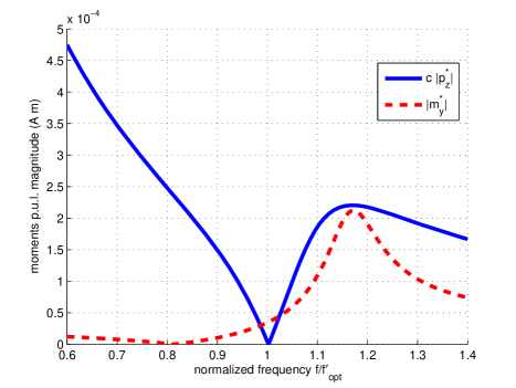
Figure 6: The magnitudes of the moments per unit length (p.u.l.) of axis z ($c~{}p^{*}_{z},m^{*}_{y}$) as functions of the normalized operating frequency $f/f^{\prime}_{opt}$. Plot parameters: $f_{0}=c/\lambda_{0}=3\cdot 10^{8}$ Hz, $f^{\prime}_{opt}=0.984f_{0}$, $g/\lambda_{0}=0.05$, $a/\lambda_{0}=0.08$, $\epsilon_{r}=60$.

After validation of the model in the vicinity of the cloaking frequency $f^{\prime}_{opt}\cong f_{opt}$, we can make exclusive use of it hereinafter. In Fig. 6 we show the magnitude variation of the two amplitudes incorporated in (35). The first one $(c|p_{z}^{*}|)$, corresponding to the electric response of the structure, is minimized (almost nullified) at $f=f^{\prime}_{opt}$ as predicted above. The second one $(|m_{y}^{*}|)$, determining the magnetic response of the cylinder, increases smoothly in the neighborhood of $f^{\prime}_{opt}$. Again, it is clearly noted that the electric moment represents the omnidirectional term of the far-field pattern, while the magnetic moment is proportional to the bipolar term as defined by expression (35). Therefore, the findings from the graphs are in accordance with those of Figs. 3 (based on the explicit field formulas), since the omnidirectional component is mitigated at the cloaking frequency.

In Figs. 7, we show the variations of the constituent parts of the quantities $cp_{z}^{*}$ and $(-m_{y}^{*})$ (real in Fig. 7 and imaginary in Fig. 7) with respect to the normalized operational frequency $f/f^{\prime}_{opt}$. The negative sign in the magnetic moment is compatible with (39), where the scattering power is written as the result of the action of two sources: one with magnitude $\Im[cp_{z}^{*}]$ and the other with magnitude $\Im[-m_{y}^{*}]$. From Fig. 7, it is apparent that the two quantities cannot give a zero sum at any frequency, since the imaginary parts (responsible for scattering losses) retain the same sign (negative) at all frequencies. Therefore, it is sensible for the optimal choice to be $f\cong f^{\prime}_{opt}$ since: (i) both imaginary parts are small as demonstrated in Fig. 7, (ii) the real part $\Re[cp_{z}^{*}]$ is nullified at $f=f^{\prime}_{opt}$ and its magnitude increases rapidly slightly far from it as shown in Fig. 7 and (iii) the real part $\Re[-m_{y}^{*}]$ does not vary considerably in the vicinity of $f=f^{\prime}_{opt}$ as again indicated in Fig. 7. When observing the frequency dispersion of the real and the imaginary parts of the electric moment, one concludes that it exhibits a typical plasma dependence tending to large negative values at low frequencies. On the other hand, the dispersion of the magnetic moment resembles a Lorentz-type curve with a resonance at higher frequencies.

In Figs. 8, we represent the real and the imaginary parts of the scattering field in the forward direction ($\phi=0$) in the far region as functions of $f/f^{\prime}_{opt}$ from expressions (5), (35), where the common factor $\sqrt{\frac{2}{\pi k_{0}\rho}}e^{-j(k_{0}\rho-\frac{\pi}{4})}$ has been dropped. By taking into account that the scattered power by the entire cylindrical structure is proportional to the real part of the electric far field as stated in (39) and observing Fig. 8, one concludes again that the perfect cloaking is not possible and only a minimization of the overall response is feasible. As far as the imaginary part of the forward-scattering quantity is concerned, it is kept moderate for $f\cong f^{\prime}_{opt}$ regardless of the method (exact or approximate) one employs to evaluate it.

6 Conclusions

An analytical model based on the equivalent moments of a cylindrical PEC rod covered by a conventional dielectric is used to analyze the minimal scattering response of the structure when it is illuminated by a normally incident plane wave (with electric field parallel to the cylinder’s axis). The adopted approximate model is reliable for moderate electrical sizes and captures the scattering effect of the illuminated object. In the vicinity of the cloaking frequency, a drastic change in the radiation pattern of the covered PEC cylinder is observed; in particular, there is a clear transition from backward to forward scattering. It has been found that the minimum scattering is achieved when the electric moment is mitigated and in that case the system radiates as a magnetic dipole line.

References

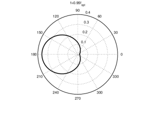
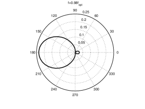
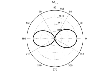
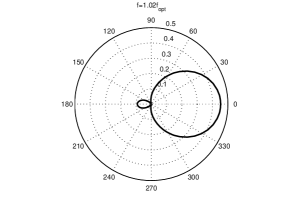
Figure 3: The normalized radiation patterns $\lim_{k_{0}\rho\rightarrow+\infty}\frac{|E_{z0,scat}(\rho,\phi)|}{|\tilde{E}_{z0,scat}(\rho,\phi)|}$ of the cylindrical structure determined from the exact field solution for: (a) $f=0.95f_{opt}$, (b) $f=0.98f_{opt}$, (c) $f=f_{opt}$, (d) $f=1.02f_{opt}$ and (e) $f=1.05f_{opt}$. Plot parameters: $f_{0}=c/\lambda_{0}=3\cdot 10^{8}$ Hz, $f_{opt}\cong 0.992f_{0}$, $g/\lambda_{0}=0.05$, $a/\lambda_{0}=0.08$, $\epsilon_{r}=60$.

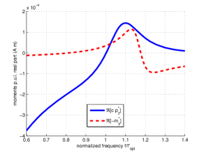
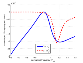
Figure 7: The: (a) real and (b) the imaginary parts of the moments $c~{}p^{*}_{z}$ and $(-m^{*}_{y})$ as functions of the normalized operating frequency $f/f^{\prime}_{opt}$. Plot parameters: $f_{0}=c/\lambda_{0}=3\cdot 10^{8}$ Hz, $f^{\prime}_{opt}=0.984f_{0}$, $g/\lambda_{0}=0.05$, $a/\lambda_{0}=0.08$.

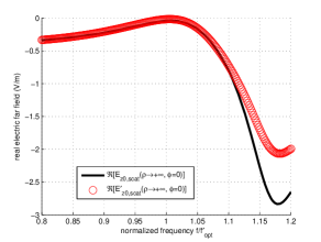
Figure 8: The: (a) real and (b) the imaginary parts of the scattered electric field in the far region along the forward direction $(\phi=0)$, using exact formulas ($\lim_{k_{0}\rho\rightarrow+\infty}E_{z0,scat}(\rho,\phi=0)$) and the approximate moments model ($\lim_{k_{0}\rho\rightarrow+\infty}E^{\prime}_{z0,scat}(\rho,\phi=0)$), as functions of the normalized operating frequency $f/f^{\prime}_{opt}$. Plot parameters: $f_{0}=c/\lambda_{0}=3\cdot 10^{8}$ Hz, $f^{\prime}_{opt}=0.984f_{0}$, $g/\lambda_{0}=0.05$, $a/\lambda_{0}=0.08$.

References

- [1] U. Leonhardt, “Optimal Conformal Mapping”, Science, vol. 312, pp. 1777-1780, 2006.
- [2] J. B. Pendry, D. Schurig and D. R. Smith, “Controlling electromagnetic fields”, Science, vol. 312, pp. 1780 1782, 2006.
- [3] P. Alitalo and S. A. Tretyakov, “Broadband electromagnetic cloaking realized with transmission-line and waveguiding structures”, Proceedings of the IEEE, vol. 99, no. 10, pp. 1646 1659, 2011.
- [4] P. Alitalo, A. E. Culhaoglu, A. V. Osipov, S. Thurner, E. Kemptner, and S. A. Tretyakov, “Experimental characterization of a broadband transmission-line cloak in free space”, IEEE Transactions on Antennas and Propagation, vol. 60, no. 10, pp. 4963-4968, 2012.
- [5] A. Alùand N. Engheta, “Achieving transparency with plasmonic and metamaterial coatings”, Physical Review E, vol. 72, no. 016623, 2005.
- [6] C. A. Valagiannopoulos and P. Alitalo, “Electromagnetic cloaking of cylindrical objects by multilayer or uniform dielectric claddings”, Physical Review B, vol. 85, no. 115402, 2012.
- [7] A. Alù, D. Rainwater and A. Kerkhoff, “Plasmonic cloaking of cylinders: finite length, oblique illumination and cross-polarization coupling”, New Journal of Physics, vol. 12, no. 103028, 2010.
- [8] A. A. Zharov and N. A. Zharova, “On the electromagnetic cloaking of (nano)particles”, Izvestiya Rossiiskoi Akademii Nauk. Seriya Fizicheskaya, vol. 74, no. 1, pp. 98-102, 2010.
- [9] G. W. Milton and N.-A. P. Nicorovici, “On the cloaking effects associated with anomalous localized resonance”, Proceedings of the Royal Society, vol. 462, pp. 3027-3059, 2006.
- [10] C. A. Valagiannopoulos, P. Alitalo and S. A. Tretyakov, “Dielectric-coated PEC cylinders which do not scatter electromagnetic waves”, Proceedings of International Conference on Electromagnetics in Advanced Applications (ICEAA) 2012, pp. 90-91, Cape Town, South Africa, 2-7 September, 2012.
- [11] C. A. Balanis, Advanced Engineering Electromagnetics, ch. 11, John Wiley and Sons, Washington, D.C., 1989.
- [12] Z. Popovic and B. D. Popovic, Introductory Electromagnetics, ch. 7, Prentice Hall, New Jersey, 1999.
- [13] C. R. Simovski and S. A. Tretyakov, “On effective electromagnetic parameters of artificial nanostructured magnetic materials”, Photonics and Nanostructures - Fundamentals and Applications, vol. 8, no. 4, pp. 254 263, 2010.
- [14] Wolfram Mathworld Documentation, “Meijer G-Function,” freely available online at: http://mathworld.wolfram.com/MeijerG-Function.html.
- [15] S. J. Orfanidis, Electromagnetic Waves and Antennas, ch. 14, freely available on-line at: http://www.ece.rutgers.edu/ orfanidi/ewa.
- [16] C. A. Valagiannopoulos, “Electromagnetic propagation into parallel-plate waveguide in the presence of a skew metallic surface”, Electromagnetics, vol. 31, no. 8, pp. 593 605, 2011.
- [17] J. J. Bowman, T. B. A. Senior, and P. L. E. Uslenghi, Electromagnetic and Acoustic Scattering by Simple Shapes, ch. 14, North-Holland Publishing Company, Amsterdam, 1969.
- [18] A. O. Karilainen and S. A. Tretyakov, “Isotropic chiral objects with zero backscattering”, IEEE Transactions on Antennas and Propagation, vol. 60, no. 9, pp. 4449-4452 , 2012.
- [19] P.-Y. Chen, J. Soric, and A. Alù, “Invisibility and cloaking based on scattering cancellation”, Advanced Materials, vol. 2012, no. 201202624, pp. 1-24, 2012.