Accurate Demarcation of Protein Domain Linkers based on Structural Analysis of Linker Probable Region

Abstract

In multi-domain proteins, the domains are connected by a flexible unstructured region called as protein domain linker. The accurate demarcation of these linkers holds a key to understanding of their biochemical and evolutionary attributes. This knowledge helps in designing a suitable linker for engineering stable multi-domain chimeric proteins. Here we propose a novel method for the demarcation of the linker based on a three-dimensional protein structure and a domain definition. The proposed method is based on biological knowledge about structural flexibility of the linkers. We performed structural analysis on a linker probable region (LPR) around domain boundary points of known SCOP domains. The LPR was described using a set of overlapping peptide fragments of fixed size. Each peptide fragment was then described by geometric invariants (GIs) and subjected to clustering process where the fragments corresponding to actual linker come up as outliers. We then discover the actual linkers by finding the longest continuous stretch of outlier fragments from LPRs. This method was evaluated on a benchmark dataset of 51 continuous multi-domain proteins, where it achieves F1 score of 0.745 ($0.83$ precision and $0.66$ recall). When the method was applied on 725 continuous multi-domain proteins, it was able to identify novel linkers that were not reported previously. This method can be used in combination with supervised / sequence based linker prediction methods for accurate linker demarcation.

1 Introduction

Complex proteins are made up of several domains that work independently or in tandem with the neighboring domains to perform the intended functions in the cellular processes [18]. The domains are linked by means of flexible structures known as domain linkers. The linkers perform a key role in cooperative inter-domain interactions, function regulation, protein stability, folding rates, and domain-domain orientation [18, 16]. The linkers are known to possess special biochemical properties such as high solvent accessibility and a typical amino acid composition, due to their role and location in the protein structure. To further our understanding on these fronts, a systematic analysis of the known linkers needs to be performed. The progress is hampered by lack of availability of known and reliable linkers. For instance, there is no database of experimentally characterized linkers something that would be of immense importance in such studies. The improved understanding of linkers and their biochemical properties is crucial in designing linkers for engineering stable multi-domain proteins.

The most reliable and accurate linker demarcation can be obtained using protein structure analysis. Crystallographers usually perform such analysis to identify domains and linkers while determining the structure of multi-domain proteins. However, in many cases, the domain linkers are not reported explicitly and we need to employ computational methods to demarcate the linkers based on sequence or structure of the protein. State of the art sequence based methods [37, 4, 11] can be used to identify a list of putative linkers and these need to be processed further using available structural features to determine the actual linkers. These methods take amino acid sequence as an input and predict domain boundaries and linkers using a domain linker index computed from amino acid propensities in the known linker region. Miyazaki and co- workers have proposed neural network [26] and support vector machine [12] based techniques using amino acid propensities to distinguish intra-domain loops from the inter-domain ones. Tanaka and co-workers used predicted secondary structure in addition to amino acid propensities to identify loops, which are further distinguished between linker and non-linker loops. Domain prediction methods are also used to predict linkers by carving out a stretch of residues in the inter domain region around domain boundary points [14, 25]. These methods tend to provide multiple linker predictions with liberal allowance for the linker boundaries and hence are not very useful for accurate protein linker demarcation. Besides, most of these methods are unable to predict helical linkers due to their assumption about linkers being loops.

George and Heringa conducted a systematic study of biochemical properties of the linkers extracted from three dimensional structures of multi-domain proteins [16, 15]. They first identify structural domains using Taylor’s method [41] and then extract linkers by branching out from domain boundaries until the branches become buried within the core of the domain or till the branch becomes 40 residues long. This method takes into account biochemical properties of linkers for their demarcation without using any of the structural features. It is well known that the linkers assume unique structures due to their placement in the protein structure [2, 33] and this forms the basis of our method. The proposed method performs accurate demarcation of linkers given a three dimensional structure and its domain definition. It first extracts a linker probable region (LPR) around domain boundary point and then performs structural analysis of the LPR to demarcate actual linker. We perform a rigorous assessment of the method using a benchmark dataset of known linkers extracted from the literature.

The rest of the paper is organized as follows: (i) The Method section explains the proposed technique in detail, (ii) The Results section presents findings and representative linkers demarcated by the proposed method. It also reports accuracy of the method and its performance vis-à-vis other state of the art methods, (iii) The Discussion section documents key contributions of the method.

2 Proposed method

The method takes a set of protein structures and the corresponding domain definitions as input and identifies the corresponding domain linkers.

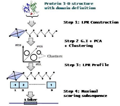
Figure 1: Schematic for protein linker demarcation: (i) Based on SCOP domain definition; we identify domain boundary point in the protein structure. A twelve residue long linker probable region (LPR) is carved out by taking six amino acids each from either domain. (ii) LPR is represented with nine overlapping tetrapeptides. (iii) Each tetrapeptide is described with a set of 15 geometric invariants (GIs). The geometric invariants are standardized to zero mean and unit standard deviation. The number of dimensions is reduced via principal component analysis (PCA). We select first 8 PCs to represent tetrapeptides. The tetrapeptides are then transformed into PC space. (iv) The hierarchical agglomerative clustering is performed to identify clusters of similar tetrapeptides. The clusters are assigned E-values based on the cluster size distribution. The E-values are standardized to zero mean and unit standard deviation, yielding structural uniqueness scores (SUS). (v) Based on the membership of a tetrapeptide to a particular cluster, we construct LPR structural profiles using SUS of the respective clusters. (vi) We perform maximally scoring subsequence discovery on top of LPR structural profile to identify the continuous stretch with maximum cumulative SUS. This stretch of tetrapeptides corresponds to the actual linker.

It can be broadly divided into the following four steps, as depicted in Figure 1, (i) Construction of linker probable regions (LPRs), (ii) Parameterization of LPRs, (iii) Generation of structure profiles by clustering LPRs, and (iv) Demarcation of actual linkers by applying dynamic programming on the structure profiles. Note that the current version of the method works only with continuous multi-domain proteins. The algorithm is given below:

0:  $\mathcal{S}=\{(S_{1},D_{1}),(S_{2},D_{2}),\ldots,(S_{n},D_{n})\}$: Set of $n$ protein structures with domain definition; and $k$: Number of positions from one domain to be included in linker probable region

0:  $\mathcal{L}=\{(S_{1},L_{1}),(S_{2},L_{2}),\ldots,(S_{n},L_{n})\}$.

1:  for each $(S_{i},D_{i})\in\mathcal{S}$ do

2:     $R$ = ExtractLPR$(S_{i},D_{i})$;

3:     $T$ = DiscretizeLPR($R$);

4:     $\mathcal{T}=\mathcal{T}+T$

5:     $\mathcal{R}=\mathcal{R}+R$

6:  end for

7:  $\mathcal{I}=\mathrm{InvariantList}()$

8:  for each $T\in\mathcal{T}$ do

9:     $\mathcal{X}=\mathcal{X}+$ InvariantGeneration($T$)

10:  end for

11:  $\mathcal{X}_{z}$ = Standardize($\mathcal{X}$)

12:  $\mathcal{X}_{pc}$ = PCA($\mathcal{X}_{z}$)

13:  $\mathcal{C}$ = Cluster($\mathcal{X}_{pc}$)

14:  for each $C\in\mathcal{C}$ do

15:     $\mathcal{E}$ = AssignEval($C$)

16:  end for

17:  for each $T\in\mathcal{T}$ do

18:     $\mathcal{U}$ = ComputeSUS($\mathcal{T},\mathcal{E}$)

19:  end for

20:  for each $R\in\mathcal{R}$ do

21:     LPRProfile = ConstructProfile($\mathcal{T},\mathcal{U}$)

22:     $L$ = GetMaximalScoringSubsequence(LPRProfile);

23:     $\mathcal{L}=\mathcal{L}+L$

24:  end for

25:  return $\mathcal{L}$

Algorithm 1 Linker Demarcation

We explain each of these steps in greater detail in the rest of the section.

2.1 Construction and parameterization of LPRs

Line 1–6 in our algorithm constructs a set of linker probable regions (LPRs), $\mathcal{R}$, from the input set of protein structures along with their domain definitions $S$. We then represent each LPR i.e. $r\in\mathcal{R}$ using a set of overlapping tertrahedrons as described below.

Let $\mathcal{S}$ be the set of protein structures along with their domain definitions. Each element of $\mathcal{S}$ is an ordered pair of structure and its domain definition. Note that since we consider only continuous multidomain proteins in our analysis, we are in a position to define domains using the position of the last amino acid residue in the domain. We will refer to the position of last amino acid as the endpoint of that domain. The set $D$ in ordered pair $(S,D)\in\mathcal{S}$ specifies endpoints of each domain in $S$. Thus, for a given structure $S$ with $e$ domains, $D=\{d_{1},d_{2},\ldots,d_{e}\}$. Here $d_{j}$ is the endpoint of domain $j$. Note that the first domain starts at the first position and the last domain ends at the last position in the protein. Any other domain $j$ with $j>1$ starts at position $d_{j-1}+1$ and ends at position $d_{j}$ in the structure. With this background, we are in a position to define LPR.

DEFINITION 1: Linker probable region (LPR) between domain $i$ and $j$ of protein $s$ is a substructure starting at position $d_{i}-k+1$ and ending at $d_{i}+k$ in $s$. It is denoted as $\mathrm{LPR}(s,i,j)$. Note that $\mathrm{LPR}(s,i,j)$ contains the end poisition $d_{i}$ of domain $i$ and its length is $2k$. The parameter $k$ is chosen based on the average linker length as reported in literature  [26, 15, 39]. LPR is the basic unit of our analysis.

EXAMPLE 1: Let $s_{j}$ be the protein structure with two domains. Let $D_{s_{j}}=\{d_{1},d_{2}\}$. $s_{j}$ has exactly one LPR that starts at position $d_{1}-k+1$ and ends at position $d_{1}+k$.

We construct a set of LPRs, $\mathcal{R}$ by extracting LPRs from $\mathcal{S}$, the input set of proteins and their domain definitions (line – 2 in algorithm). Note that all the LPRs in $\mathcal{R}$ are of equal length $2k$. The backbone structure of each LPR is approximated with its $C_{\alpha}$ coordinates  [42]. Thus, $R$ is a set of $2k$ amino acid residues along with their positions in the structure as given by the $x,y,z$ coordinates. Now we will describe a procedure DiscretizeLPR (line – 3 in our algorithm). Each $r\in\mathcal{R}$ is discretized into a sequence of $2k-3$ overlapping tetrapeptides $T=t_{1,2,3,4},t_{2,3,4,5},\ldots,t_{(2k-3),(2k-2),(2k-1),(2k)}$. Note that the consecutive tetrapeptides $t_{i}$ and $t_{i+1}$ in sequence $T$ share an overlap of three amino acid residues. Each tetrapeptide in $T$ is added to $\mathcal{T}$, which is a global set of tetrapeptides obtained by discretizing LPRs (line – 4 in algorithm).

Each tetrapeptide $t\in\mathcal{T}$ represents a tetrahedral geometry and is described by a fixed suite of $g$ descriptors, which are invariant under transformations such as rotation and translation [28, 45, 44, 42]. These descriptors are referred to as geometric invariants (GIs) in the subsequent text. The suite of invariants is carefully chosen after extensive trial and error on training data to address the following two issues: (a) for superimposable tetrapeptides, the invariants must be similar within a tolerance limit $\delta$; and (b) for a pair of non-superimposable tetrapeptides $t_{1}$ and $t_{2}$, there must be at least one geometric invariant such that $f(t_{1})$ is not similar to $f(t_{2})$. Here $f$ is a function that calculates a specific GI. We represent each tetrapeptide $t\in\mathcal{T}$ with a suite of fifteen GIs (line – 7). The detailed method for calculating these GIs is given in our previous work [44, 42] (line – 9).

1. Nine GIs are calculated based on the tetrahedral geometry of $t$ and they represent signed volume and perimeter of $t$, length of each edge in $t$. Since there are in all six edges so we have six GIs corresponding to the length. One more invariant is computed based on the sum of distance of each vertex of $t$ from the centroid of all the vertices. Let $V_{t}$ be the set of all vertices in $t$. The $i$-th vertex $v_{i}\in V_{t}$ gives $x,y,z$ coordinate position of $i$-th amino acid residue in $t$. The centroid is calculated as follows:

   $$\mu=\frac{1}{n}\sum_{\forall v\in V_{t}}v$$

   and the sum of distance from centroid is calculated as

   $$\sum_{\forall v\in V_{t}}(v-\mu)$$

2. The remaining six invariants for $t$ are calculated by forming three triangles using vertices in $V_{t}$. The three traingles are as follows: $v_{1},v_{2},v_{3}$, $v_{1},v_{3},v_{4}$ and $v_{1},v_{2},v_{4}$. We calculate area and perimeter for each of these traingles, thus accounting for the six remaining invariants.

.

Further we standardize $\mathcal{X}$ to zero mean and unit standard deviation values. Let $\mathcal{X}_{z}$ be the set of standardized GIs for $\mathcal{T}$ (Line – 11). We perform Principal Component Analysis (PCA) to get rid of correlations between GIs [43]. PCA gives a new set of orthogonal dimensions, which are linear combinations of the original dimensions (GIs in this case). We selected first $m$ significant principal components (PCs) to represent the tetrapeptides. Let $\mathcal{X}_{pc}$ be the set of tetrapeptides represented using $m$ PCs (Line – 12).

2.2 Structural profiling of LPRs

Since the linkers are unstructured regions, we believe that the corresponding tetrapeptides share structural similarity with fewer other tetrapeptides. On the other hand, the tetrapeptides from non-linker region are expected to share structural similarity with a large number of other tetrapeptides. Our objective is to determine the groups of structurally similar tetrapeptides through clustering process and utilize this knowledge towards the demarcation of actual linkers. We perform clustering of a set of tetrapeptides $\mathcal{X}_{pc}$, which are represented using $m$ PCs as explained earlier (Line – 13). The clustering is carried out via Matlab implementation of hierarchical agglomerative clustering (HAC) [38]. We use euclidean distance as a measure of similarity and ward linkage [38] for merging the nodes in the clustering tree. The optimal cut in the resulting dendrogram is determined by using inconsistency parameter, which leads to the discovery of a set of clusters $\mathcal{C}$. The inconsistency parameter compares each link in the cluster hierarchy with the adjacent links to determine natural cluster division in the dataset [38]. The clustering process assigns each tetrapeptide to exactly one cluster.

Once the clustering process is over, we obtain the distribution of cluster sizes, which is used to assign e-value to each cluster based on its size (Lines 14–16). The e-value for a cluster $C\in\mathcal{C}$ with size $|C|$ is calculated as $\alpha/|\mathcal{C}|$, where $\alpha$ be the number of clusters in $\mathcal{C}$ with size greater than $|C|$ and $|\mathcal{C}|$ is the total number of clusters. Note that the large clusters are expected to contain tetrapeptides corresponding to the non-linker regions, while the smaller clusters are more likely to contain tetrapeptides corresponding to the linker region. The e-values are normalized to zero mean and unit standard deviation to obtain structural uniqueness score (SUS) of the cluster. The large clusters have lower SUS, while the smaller clusters have higher SUS. The smallest SUS is assigned to the largest clusters, while the largest SUS is assigned to the singleton clusters. Thus, the SUS indicates the structural uniqueness of the cluster and its propensity to be a part of the actual linker. Each tetrapeptide in the cluster is assigned the SUS of that cluster (Lines 17–19). The structural profile of an LPR is represented using the SUS of its constituent tetrapeptides (Line 21).

2.3 Protein domain linker demarcation

Given the structural profile of an LPR, we are interested in finding the longest continuous stretch of tetrapeptides with the highest cumulative SUS. Note that such tetrapeptides; being highly unstructured; appear as outliers in the clustering process. Hence, the stretch is demarcated as a linker between the domains. We are required to enumerate all possible stretches in order to find the one with the greatest cumulative SUS. The problem is tackled by using linear time dynamic programming algorithm proposed by Ruzzo and Tompa  [ruzzo:1999] (Line – 22). The algorithm takes a sequence of real numbers as input and generates non-overlapping, contiguous subsequences having greatest total score. Here, the algorithm takes the structural profile of an LPR as input, which is a sequence of nine SUS scores of the constituent tetrapeptides $(u_{1},u_{2},\ldots,u_{2k-3})$, where $u_{i}\in R$. Let $Q$ be the set of all possible subsequences of tetrapeptides. The cumulative SUS for each subsequence is obtained by simply summing the SUS of the constituent tetrapeptides. Let $\mathrm{\texttt{CumSUS}}(q)$ be the function that gives cumulative score for the subsequence $q\in Q$. The GetMaximalScoringSubsequence procedure finds the subsequence with the greatest cumulative SUS (Line – 22). We declare such a subsequence as a domain linker. In case of a tie, a subsequence with the closest proximity to the domain boundary is declared as a domain linker. Thus,

$$L=\mathrm{argmax}_{q\in Q}\mathrm{\texttt{CumSUS}}(q)$$

2.4 Evaluation of proposed method

It is of interest to evaluate the accuracy of the proposed method. In the absence of linker database and due to a lot of subjectivity in linker detection by visual examination, we decided to extract experimentally reported linkers from the literature. We first selected research papers based on PDB reference record of each protein in our input dataset. We then manually read the literature for extracting information about experimentally detected linkers. We succeded in extracting linker information about 51 proteins out of 725 proteins in the input set (Supplementary Table 1). These linkers form an evaluation set for the benchmark studies.

After demarcating the linkers using the proposed method, we compare them with the literature reported linkers. We compute the accuracy of demarcation residue wise as follows: If the residue marked as a part of the linker also happens to be the part of the literature reported linker, we count it as a true positive match, else it is counted as a false positive match. If the residue that is part of the literature reported linker, but is not present in the linker marked by the proposed method, it is counted as a false negative match. Let $TP$ denotes the number of correctly demarcated linker residues, $FP$ denotes the number of incorrectly demarcated linker residues, which are actually non-linker residues and $FN$ denotes the number of actual linker residues, which were not included in demarcated linker region. Based on $TP,TN$ and $FN$, we compute precision and recall of the proposed method as follows:

$$\mathrm{Recall}=\frac{TP}{TP+FN}$$

$$\mathrm{Precision}=\frac{TP}{TP+FP}$$

We also compute $F1$ measure, which is harmonic mean of precision and recall, for the proposed method.

3 Results

3.1 Dataset preparation and structural profiling of LPRs

We have selected 610 continuous multi-domain proteins from the ASTRAL 40 [8] dataset version 1.69. Out of 610 selected proteins, we have 505 two domain, 95 three domain and 10 four domain proteins. Based on the SCOP [29] domain definition, we selected a stretch of 6 amino acids on either side of the domain boundary point to extract LPR of length 12 for each domain connection. Thus, we obtain 725 LPRs from the input protein domains. Each LPR is represented by nine overlapping tetrapeptides with an overlap of three residues between the consecutive tetrapeptides. Each tetrapeptide is represented with fifteen geometric invariants (GIs) as described earlier. Thus, we obtain 6525 tetrapeptides represented in 15 dimensional space spanned by GIs. This dataset is subjected to PCA, which reveals that the first 8 PCs cover 99% variance in the data. The tetrapeptides were then transformed into a reduced dimensional space spanned by first 8 PCs. The transformed dataset of tetrapeptides is subjected to hierarchical clustering algorithm (Matlab implementation). The resulting dendrogram was cut based on inconsistency parameter to obtain 2188 clusters. The distribution of clusters in terms of their size is shown in Table 1. Note that we obtain a large number of smaller clusters, approximately 50%, with size less than three members. The largest cluster contains 14 tetrapeptides.

Cluster Size	Number of Clusters
1	207
2	899
3	520
4	269
5	131
6	58
7	45
8	23
9	13
10	9
11	3
12	4
13	4
14	3

Table 1: Distribution of clusters of tetrapeptides according to their size.

The larger clusters are assigned smaller e-values, while the smaller clusters are assigned larger e-values. We then constructed the structural profile of LPRs using the SUS of the corresponding tetrapeptides. The structural profiles, each of length nine, were subjected to a maximally scoring subsequence finding algorithm to demarcate the actual linkers. We were able to demarcate 692 domain linkers from 725 input LPRs. In the remaining 33 cases, we observed that these LPRs contain tetrapeptides with lower SUS. The distribution of linker lengths is shown in Table 2. We found that the average length of the linker detected by the proposed method is 5.3 residues.

Linker Length	4	5	6	7	8	9	10	11
Linker Count	286	178	93	67	31	19	11	7

Table 2: Distribution of linkers according to their lengths. The linkers are obtained via the proposed method

3.2 Comparison with other methods

We were interested in comparing the proposed method against the state of the art methods to assess its performance. We used 51 literature reported linkers for the comparative analysis. The same set was used for evaluating the proposed method. We have selected the following methods in the comparison study: Ebina et al. [12], GM[14] and CHOP [25]. Note that the direct comparison is inappropriate since most of these methods predict putative domain linkers from the sequence characteristics, while our method demarcates domain linkers by analyzing structural characteristics of LPRs. Moreover most of these methods predict multiple putative linkers with certain flexibility on start and end positions. From these predictions, we selected the most appropriate linker based on the known domain definition and used it for the comparison. A representative examples of the linkers identified by different methods on the input set are reported in Table 3. The complete list can be obtained from Supplementary Table 1. These predictions are matched with the actual linkers and the accuracy is calculated in terms of F1 score, which is the harmonic mean of precision and recall. The comparative performance of the proposed method is given in Table 4. The proposed method achieves overall recall of 0.66 and precision of 0.83 on the benchmark dataset. It significantly outperforms state of the art methods in terms of the number of linkers identified as well as the accuracy of the predictions.

PDB ID	Lit. Ref.	Actual Linker	Proposed Method	Ebina et. al. [12]	GM [14]	CHOP [25]
1h03	[46]	65-68	64-70	47-73	50-70	66-67
1eqf	[21]	1495-1502	1492-1503	1521-1540	1504-1524	1496-1515
1fcd	[9]	76-84	77-80	75-83	97-117	78-79
1vi7	[31]	134-139	133-138	132-138	156-176	137-138
1fp5	[48]	436-440	438-442	420-461	436-456	446-447
1fx7	[13]	141-150	143-146	139-147	137-157	139-151
1f1b	[23]	95-101	95-102	93-102	88-108	100-101
1f14	[5]	201-206	201-204	193-206	249-269	218-222
1jt6	[34]	72-74	70-73	73-76	123-143	51-52
1m3y	[30]	213-224	220-226	213-226	244-264	223-224
1eem	[6]	98-107	100-104	97-112	82-102	125-126
1g3n	[22]	142-150	149-152	133-136	193-213	150-151
1l3l	[50]	163-174	168-172	166-170	146-166	171-172
1gnw	[32]	78-92	84-87	106-113	107-127	88-92
1dkz	[51]	503-508	501-512	535-540	459-479	541-542
1e79	[17]	95-105	96-101	66-80	61-81	117-118
1gpj	[27]	142-148	141-144	136-142	153-173	142-146
1hf2	[10]	96-102	95-99	82-87	132-152	100-102
1hlv	[40]	65-74	64-67	56-57	70-90	66-72
1hv8	[35]	208-214	207-210	249-253	300-320	208-211
1hyr	[24]	175-184	178-181	175-194	185-205	183-184
1jb9	[1]	156-164	158-161	159-164	155-175	158-159
1jbw	[36]	295-300	291-300	278-288	345-365	298-299
1k0d	[7]	197-205	195-198	175-186	195-215	210-211
1k0m	[19]	89-100	92-97	90-95	96-116	97-98

Table 3: The table contains a representative examples of linkers extracted by the proposed method. We have also shown actual linker as extracted from the literature as well as the linkers predicted by state of the art methods. The column Lit. Ref. provides the literature reference for the actual linker.

Method	Precision	Recall	F1 Score	No. of Predictions
Proposed Method	0.83	0.66	0.74	51
Ebina et. al. [12]	0.48	0.57	0.52	29
CHOP [25]	0.35	0.39	0.37	36
GM [14]	0.19	0.50	0.27	22

Table 4: Performance of various methods on the benchmark dataset of 51 linkers

We further compared our method against DomCut, which predicts the domain cut point based on domain linker index. Note that DomCut does not predict the start and the end position of linker. The DomCut prediction is taken as a correct prediction if the predicted domain cut point falls within the actual linker. Out of 51 linkers, we found that DomCut predicts correctly in 13 cases and does not predict the domain cut point in 14 cases. In the remaining cases, the predicted cut point does not fall inside the actual linker.

We computed the agreement between our method against the linker database of George and Heringa [16, 15], which gives linker predictions for 79 proteins in our input dataset. Note that linker prediction is available for few proteins from evaluation set used earlier and hence it is not used for the comparison between the two methods. We found that the predictions partially agree in 55 cases and completely disagree in 24 cases. Reasonable agreement ($>75\%$) was obtained in 5 cases, while medium agreement ($<75\%$ and $>40\%$) was obtained in 29 cases and weak agreement was observed in the remaining cases.

3.3 Representative linkers

The examples of demarcated linkers by the proposed method are shown in Figures 2A–2J. Since the method use LPR for demarcation, the entire 3-D structure of corresponding domains is not shown. Instead, a stretch of 16 amino acids on either side of the domain boundary point is shown to maintain clarity of representation. Here we describe a few representative linkers.

Example of literature reported linkers, also demarcated by our method

1. Streptococcus pneumonia SP14.3 (PDB Code: 1IB8)
   Streptococcis pneumonia is a deadly human pathogen causing high mortality and morbidity rates  [49]. SP14.3 is a key protein responsible for growth of the pathogene. The three-dimensional structure of SP14.3 contains a very short linker of size 3 between residues 88-90 with a moderate flexibility. Our method predicts the linker exactly at the same place as reported by Yu et. al.  [49]. The linker plays role in relative orientation of domains and maintaining rotational cooorelation of domains.

2. Yeast Sec18p (PDB Code: 1CR5)
   Yeast Sec18p is a hexameric ATPase with a central role in vesicle trafficking [3]. The reported linker is located between residues 104-113 and is flexible in its structure. The SNAP binding site is located opposite to the linker. It connects two beta rich sub domains and is likely to facilitate different sub-domain orientation. Our method detected the linker between residues 104-111, which is enclosed within the literature reported linker (Figure 2A).

3. TnsA (PDB Code: 1F1Z)
   TnsA carries out DNA breakage at 5’ end of transposon. It contains a six sized loop linker between residues 165-170 that connects two domains of homodimeric endonuclease enzymes [20]. Our method predicted eight sized linker between residues 164-171 (Figure 2B). The linker is likely to play a role in cooperative domain binding.

Examples of novel linkers that are not reported in literature
Figure 2G shows the novel linker in Ornithine transcarbamoylase (1DUV) which is not reported in the literature. Fascin (1DFC) has three domains, and the two linkers delimiting these domains were demarcated accurately (Figures 2H and 2I). Spectrin beta chain (1S35) is an all alpha protein with an alpha-helical linker between two domains (Figure 2J). A helical conformation of the linker region is compatible with a variety of different twist angles between Spectrin repeats, leading to many different conformations.

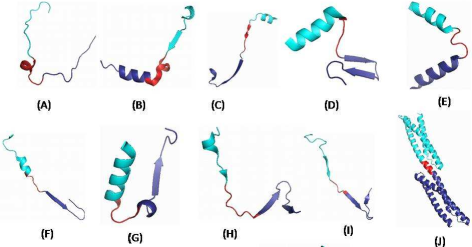
Figure 2: Different categories of substructures predicted as linkers. The segment of the N- terminal domain is shown in cyan whereas the segment of the C-terminal domain is shown in blue. The segment of the structure demarcated as a linker is shown in red. (A) 1CR5 [N–terminal domain of Sec18p], helical linker [LEU 104 -– GLN 111]; (B) 1F1Z [TnsA endonuclease], linker [THR 164 -– VAL 171]; (C) 1VI7 [Hypothetical protein YigZ], beta linker [THR 133 –- PRO 138]; (D) 1P2F [Response regulator DrrB from Thermotoga maritime], loop linker [GLU 118 -– GLY 121]; (E) 1R89 [tRNA nucleotidyltransferase], loop linker [GLY 139 –- GLY 143]; (F) 1DT9 [Eukaryotic peptide chain release factor subunit 1], novel linker [LEU 140 -– SER 144]; (G) 1DUV [Ornithine transcarbamoylase], novel linker [LEU 148 –- ALA 152]; (H) 1DFC [Fascin], loop linker between domain 1 and domain 2 [HIS 1135 -– GLN 1141]; (I) 1DFC [Fascin], loop linker between domain 2 and domain 3 [SER 1259 -– GLN 1262]; (J) 1S35 [Spectrin beta chain], helical linker [THR 1163 – PHE 1170]. The figures are prepared using PyMOL (http://www.pymol.org).

4 Discussion

We proposed a novel objective method for accurate demarcation of linkers. The method takes three dimensional protein structure and domain definition as an input and provides accurate linker demarcation. This is the first instance where structural aspects are rigorously analyzed in the linker demarcation task. The earlier methods have used biochemical and sequence properties for the same task. Since the proposed method provides structural perspective in the demarcation, it can be used in tandem with the other methods reported in literature.

As stated earlier, accurate domain linker demarcation is a key to understand their biochemical properties. Given a three dimensional structure and its domain definition, the linkers can be demarcated either through direct visualization or through objective automated methods reported in the literature [16, 26, 37, 4, 11, 12]. Visualization methods are often subjective, while automated methods demarcate linkers only approximately. The proposed method demarcates the linker more precisely than the other methods as demonstrated on the benchmark dataset. Our method outperforms other methods with F1 score of $0.745$ (precision 0.83 and recall 0.66) on the benchmark dataset.

The method is also the first of its kind in exploiting biological knowledge about structural uniqueness of linkers. Since the linkers possess flexible structure, their constituent fragments are unique and appear as outliers during clustering process [47]. Since the outliers are assigned the maximum SUS, the stretch of fragments with maximum cumulative SUS corresponds to the actual linker. The discovery of such stretch was performed using an efficient linear time dynamic programming algorithm.

The proposed method has following configurable parameters, which can be adjusted to achieve desired results: (i) $k$ which affects the length of LPRs and (ii) the length of the peptide fragment. The current study uses LPRs of length 12, tetrahedron as a choice for local structure and clusters of tetrahedrons in LPRs. The length of LPR was decided based on the prior reports of average linker lengths [16, 26, 39]. Flexibility can be added to LPR selection with the help of other methods reported in the literature. For instance, we can use Taylor’s method [41] as applied by [16] to come up with more appropriate LPRs. The LPRs thus obtained can be processed further with the help of the proposed method to demarcate accurate linkers. In the present study, we extract tetra-peptides from LPRs and perform the clustering. The clusters are then assigned SUS based on cluster size distribution. Our method is able to find linkers with irregular or unique structure. It is also able to detect linkers containing alpha-helices and beta-strands with structural purturbations. Due to these purturbations, these tetrapeptides are part of smaller clusters, which are often assigned higher SUS and hence our method is able to detect linkers containing such structures. However, our method is unable to detect linkers made up of regular alpha-helices and beta-strands, since the regular structures tend to form larger clusters and usually have smaller SUS compared to the irregular structures.

Finally, we plan to construct a database of linkers demarcated via the proposed method. The database will help to further our understanding of biochemical properties of linkers and help to design better linkers while engineering multi-domain proteins. We are planning to use insights about linkers from this work to develop a sequence based linker prediction method. This can be useful in predicting protein domains by virtue of linker prediction.

5 Acknowledgement

We are grateful to Prof. Pramod Wangikar - IIT Bombay and Mr. Nivruti Hinge for their useful discussions and timely help. We thank Michael Tress for his useful comments on the manuscript. This work is supported by Innovative Young Biotechnologist Award (IYBA) grant from Department of Biotechnology of Government of India to AVT.

References

- [1] A. Aliverti, R. Faber, C. M. Finnerty, C. Ferioli, V. Pandini, A. Negri, P. A. Karplus, and G. Zanetti. Biochemical and crystallographic characterization of ferredoxin-NADP(+) reductase from nonphotosynthetic tissues. Biochemistry, 40:14501–14508, 2001.
- [2] P. Argos. An investigation of oligopeptides linking domains in protein tertiary structures and possible candidates for general gene fusion. J Mol Biol, 211:943–958, 1990.
- [3] S. M. Babor and D. Fass. Crystal structure of the Sec18p N-terminal domain. Proc Natl Acad Sci U S A, 96:14759–14764, 1999.
- [4] K. Bae, B. K. Mallick, and C. G. Elsik. Prediction of protein interdomain linker regions by a hidden Markov model. Bioinformatics, 21:2264–2270, 2005.
- [5] J. J. Barycki, L. K. O’Brien, A. W. Strauss, and L. J. Banaszak. Sequestration of the active site by interdomain shifting. Crystallographic and spectroscopic evidence for distinct conformations of L-3-hydroxyacyl-CoA dehydrogenase. J Biol Chem, 275:27186–27196, 2000.
- [6] P. G. Board, M. Coggan, G. Chelvanayagam, S. Easteal, L. S. Jermiin, G. K. Schulte, D. E. Danley, L. R. Hoth, M. C. Griffor, A. V. Kamath, M. H. Rosner, B. A. Chrunyk, D. E. Perregaux, C. A. Gabel, K. F. Geoghegan, and J. Pandit. Identification, characterization, and crystal structure of the Omega class glutathione transferases. J Biol Chem, 275:24798–24806, 2000.
- [7] L. Bousset, H. Belrhali, R. Melki, and S. Morera. Crystal structures of the yeast prion Ure2p functional region in complex with glutathione and related compounds. Biochemistry, 40:13564–13573, 2001.
- [8] S. E. Brenner, P. Koehl, and M. Levitt. The ASTRAL compendium for protein structure and sequence analysis. Nucleic Acids Res, 28:254–256, 2000.
- [9] Z. W. Chen, M. Koh, G. Van Driessche, J. J. Van Beeumen, R. G. Bartsch, T. E. Meyer, M. A. Cusanovich, and F. S. Mathews. The structure of flavocytochrome c sulfide dehydrogenase from a purple phototrophic bacterium. Science, 266:430–432, 1994.
- [10] S. C. Cordell, R. E. Anderson, and J. Löwe. Crystal structure of the bacterial cell division inhibitor MinC. EMBO J, 20:2454–2461, 2001.
- [11] M. Dumontier, R. Yao, H. J. Feldman, and C. W. V. Hogue. Armadillo: domain boundary prediction by amino acid composition. J Mol Biol, 350:1061–1073, 2005.
- [12] T. Ebina, H. Toh, and Y. Kuroda. Loop-length-dependent SVM prediction of domain linkers for high-throughput structural proteomics. Biopolymers, 92:1–8, 2009.
- [13] M. D. Feese, B. P. Ingason, J. Goranson-Siekierke, R. K. Holmes, and W. G. Hol. Crystal structure of the iron-dependent regulator from Mycobacterium tuberculosis at 2.0-A resolution reveals the Src homology domain 3-like fold and metal binding function of the third domain. J Biol Chem, 276:5959–5966, 2001.
- [14] O. V. Galzitskaya and B. S. Melnik. Prediction of protein domain boundaries from sequence alone. Protein Sci, 12:696–701, 2003.
- [15] R. A. George and J. Heringa. An analysis of protein domain linkers: Their classification and role in protein folding. Protein Eng, 15:871–879, 2002.
- [16] R. A. George and J. Heringa. SnapDRAGON: a method to delineate protein structural domains from sequence data. J Mol Biol, 316:839–851, 2002.
- [17] C. Gibbons, M. G. Montgomery, A. G. Leslie, and J. E. Walker. The structure of the central stalk in bovine F(1)-ATPase at 2.4 A resolution. Nat Struct Biol, 7:1055–1061, 2000.
- [18] R. S. Gokhale and C. Khosla. Role of linkers in communication between protein modules. Curr Opin Chem Biol, 4:22–27, 2000.
- [19] S. J. Harrop, M. Z. DeMaere, W. D. Fairlie, T. Reztsova, S. M. Valenzuela, M. Mazzanti, R. Tonini, M. R. Qiu, L. Jankova, K. Warton, A. R. Bauskin, W. M. Wu, S. Pankhurst, T. J. Campbell, S. N. Breit, and P. M. Curmi. Crystal structure of a soluble form of the intracellular chloride ion channel CLIC1 (NCC27) at 1.4-A resolution. J Biol Chem, 276:44993–45000, 2001.
- [20] A. B. Hickman, Y. Li, S. V. Mathew, E. W. May, N. L. Craig, and F. Dyda. Unexpected structural diversity in dna recombination: the restriction endonuclease connection. Mol Cell, 6:1025–1034, 2000.
- [21] R. H. Jacobson, A. G. Ladurner, D. S. King, and R. Tjian. Structure and function of a human TAFII250 double bromodomain module. Science, 288:1422–1425, 2000.
- [22] P. D. Jeffrey, L. Tong, and N. P. Pavletich. Structural basis of inhibition of CDK-cyclin complexes by INK4 inhibitors. Genes Dev, 14:3115–3125, 2000.
- [23] L. Jin, B. Stec, and E. R. Kantrowitz. A cis-proline to alanine mutant of E. coli aspartate transcarbamoylase: Kinetic studies and three-dimensional crystal structures. Biochemistry, 39:8058–8066, 2000.
- [24] P. Li, D. L. Morris, B. E. Willcox, A. Steinle, T. Spies, and R. K. Strong. Complex structure of the activating immunoreceptor NKG2D and its MHC class I-like ligand MICA. Nat Immunol, 2:443–451, 2001.
- [25] J. Liu and B. Rost. CHOP proteins into structural domain-like fragments. Proteins, 55:678–688, 2004.
- [26] S. Miyazaki, Y. Kuroda, and S. Yokoyama. Characterization and prediction of linker sequences of multi-domain proteins by a neural network. J Struct Funct Genomics, 2:37–51, 2002.
- [27] J. Moser, W. D. Schubert, V. Beier, I. Bringemeier, D. Jahn, and D. W. Heinz. V-shaped structure of glutamyl-tRNA reductase, the first enzyme of tRNA-dependent tetrapyrrole biosynthesis. EMBO J, 20:6583–6590, 2001.
- [28] D. Mumford, J. Fogarty, and F. Kirwan. Geometric invariant theory. Ergebnisse der Mathematik und ihrer Grenzgebiete. Springer-Verlag, 1994.
- [29] A. G. Murzin, S. E. Brenner, T. Hubbard, and C. Chothia. SCOP: a structural classification of proteins database for the investigation of sequences and structures. J Mol Biol, 247:536–540, 1995.
- [30] N. Nandhagopal, A. A. Simpson, J. R. Gurnon, X. Yan, T. S. Baker, M. V. Graves, J. L. Van Etten, and M. G. Rossmann. The structure and evolution of the major capsid protein of a large, lipid-containing DNA virus. Proc Natl Acad Sci U S A, 99:14758–14763, 2002.
- [31] F. Park, K. Gajiwala, G. Eroshkina, E. Furlong, D. He, Y. Batiyenko, R. Romero, J. Christopher, J. Badger, J. Hendle, J. Lin, T. Peat, and S. Buchanan. Crystal structure of YIGZ, a conserved hypothetical protein from Escherichia coli k12 with a novel fold. Proteins, 55:775–777, 2004.
- [32] P. Reinemer, L. Prade, P. Hof, T. Neuefeind, R. Huber, R. Zettl, K. Palme, J. Schell, I. Koelln, H. D. Bartunik, and B. Bieseler. Three-dimensional structure of glutathione S-transferase from Arabidopsis thaliana at 2.2 A resolution: Structural characterization of herbicide-conjugating plant glutathione S-transferases and a novel active site architecture. J Mol Biol, 255:289–309, 1996.
- [33] C. R. Robinson and R. T. Sauer. Optimizing the stability of single-chain proteins by linker length and composition mutagenesis. Proc Natl Acad Sci U S A, 95:5929–5934, 1998.
- [34] M. A. Schumacher, M. C. Miller, S. Grkovic, M. H. Brown, R. A. Skurray, and R. G. Brennan. Structural mechanisms of QacR induction and multidrug recognition. Science, 294:2158–2163, 2001.
- [35] R. M. Story, H. Li, and J. N. Abelson. Crystal structure of a DEAD box protein from the hyperthermophile Methanococcus jannaschii. Proc Natl Acad Sci U S A, 98:1465–1470, 2001.
- [36] X. Sun, J. A. Cross, A. L. Bognar, E. N. Baker, and C. A. Smith. Folate-binding triggers the activation of folylpolyglutamate synthetase. J Mol Biol, 310:1067–1078, 2001.
- [37] M. Suyama and O. Ohara. DomCut: prediction of inter-domain linker regions in amino acid sequences. Bioinformatics, 19:673–674, 2003.
- [38] P. Tan, M. Steinbach, and V. Kumar. Introduction to data mining. Pearson Addison Wesley, 2006.
- [39] T. Tanaka, Y. Kuroda, and S. Yokoyama. Characteristics and prediction of domain linker sequences in multi-domain proteins. J Struct Funct Genomics, 4:79–85, 2003.
- [40] Y. Tanaka, O. Nureki, H. Kurumizaka, S. Fukai, S. Kawaguchi, M. Ikuta, J. Iwahara, T. Okazaki, and S. Yokoyama. Crystal structure of the CENP-B protein-DNA complex: the DNA-binding domains of CENP-B induce kinks in the CENP-B box DNA. EMBO J, 20:6612–6618, 2001.
- [41] W. R. Taylor. Protein structural domain identification. Protein Eng., 3:203–216, 1999.
- [42] A. V. Tendulkar, A. A. Joshi, M. A. Sohoni, and P. P. Wangikar. Clustering of protein structural fragments reveals modular building block approach of nature. J Mol Biol, 338:611–629, 2004.
- [43] A. V. Tendulkar, M. A. Sohoni, B. Ogunnaike, and P. P. Wangikar. A geometric invariant-based framework for the analysis of protein conformational space. Bioinformatics, 21:3622–3628, 2005.
- [44] A. V. Tendulkar, P. P. Wangikar, M. A. Sohoni, V. V. Samant, and C. Y. Mone. Parameterization and classification of the protein universe via geometric techniques. J Mol Biol, 334:157–172, 2003.
- [45] H. Weyl. The classical groups: their invariants and representations. Princeton landmarks in mathematics and physics. Princeton University Press, 1997.
- [46] P. Williams, Y. Chaudhry, I. G. Goodfellow, J. Billington, R. Powell, O. B. Spiller, D. J. Evans, and S. Lea. Mapping CD55 function. The structure of two pathogen-binding domains at 1.7 A. J Biol Chem, 278:10691–10696, 2003.
- [47] W. Wriggers, S. Chakravarty, and P. A. Jennings. Control of protein functional dynamics by peptide linkers. Biopolymers, 80:736–746, 2005.
- [48] B. A. Wurzburg, S. C. Garman, and T. S. Jardetzky. Structure of the human IgE-Fc C epsilon 3-C epsilon 4 reveals conformational flexibility in the antibody effector domains. Immunity, 13:375–385, 2000.
- [49] L. Yu, A. H. Gunasekera, J. Mack, E. T. Olejniczak, L. E. Chovan, X. Ruan, D. L. Towne, C. G. Lerner, and S. W. Fesik. Solution structure and function of a conserved protein SP14.3 encoded by an essential Streptococcus pneumoniae gene. J Mol Biol, 311:593–604, 2001.
- [50] R. Zhang, T. Pappas, J. L. Brace, P. C. Miller, T. Oulmassov, J. M. Molyneaux, J. C. Anderson, J. K. Bashkin, S. C. Winans, and A. Joachimiak. Structure of a bacterial quorum-sensing transcription factor complexed with pheromone and DNA. Nature, 417:971–974, 2002.
- [51] X. Zhu, X. Zhao, W. F. Burkholder, A. Gragerov, C. M. Ogata, M. E. Gottesman, and W. A. Hendrickson. Structural analysis of substrate binding by the molecular chaperone DnaK. Science, 272:1606–1614, 1996.