Convergence of the largest eigenvalue of normalized sample covariance matrices when $p$ and $n$ both tend to infinity with their ratio converging to zero

Abstract

Let ${\mathbf{X}}_{p}=({\mathbf{s}}_{1},\ldots,{\mathbf{s}}_{n})=(X_{ij})_{p\times n}$ where $X_{ij}$’s are independent and identically distributed (i.i.d.) random variables with $EX_{11}=0,EX_{11}^{2}=1$ and $EX_{11}^{4}<\infty$. It is showed that the largest eigenvalue of the random matrix ${\mathbf{A}}_{p}=\frac{1}{2\sqrt{np}}({\mathbf{X}}_{p}{\mathbf{X}}_{p}^{\prime}-n{\mathbf{I}}_{p})$ tends to $1$ almost surely as $p\rightarrow\infty,n\rightarrow\infty$ with $p/n\rightarrow 0$.

and

1 Introduction

Consider the sample covariance type matrix ${\mathbf{S}}=\frac{1}{n}{\mathbf{X}}_{p}{\mathbf{X}}_{p}^{\prime}$, where ${\mathbf{X}}_{p}=({\mathbf{s}}_{1},\ldots,{\mathbf{s}}_{n})=(X_{ij})_{p\times n}$ and $X_{ij},i=1,\ldots,p,j=1,\ldots,n$, are i.i.d. random variables with mean zero and variance 1. For such a matrix, much attention has been paid to asymptotic properties of its eigenvalues in the setting of $p/n\rightarrow c>0$ as $p\rightarrow\infty$ and $n\rightarrow\infty$. For example, its empirical spectral distribution (ESD) function $F^{{\mathbf{S}}}(x)$ converges with probability one to the famous Marčenko and Pastur law (see [9] and [8]). Here, the ESD for any matrix ${\mathbf{A}}$ with real eigenvalues $\lambda_{1}\leq\lambda_{2}\leq\cdots\leq\lambda_{p}$ is defined by

$$F^{{\mathbf{A}}}(x)=\frac{1}{p}\#\{i\colon\ \lambda_{i}\leq x\},$$

where $\#\{\cdots\}$ denotes the number of elements of the set. Also, with probability one its maximum eigenvalue and minimum eigenvalue converge, respectively, to the left end point and right end point of the support of Marčenko and Pastur’s law (see [7] and [3]).

In contrast with asymptotic behaviors of ${\mathbf{S}}$ in the case of $p/n\rightarrow c$, the asymptotic properties of ${\mathbf{S}}$ have not been well understood when $p/n\rightarrow 0$. The first breakthrough was made in Bai and Yin [2]. They considered the normalized matrix

$${\mathbf{A}}_{p}=\frac{1}{2\sqrt{np}}({\mathbf{X}}_{p}{\mathbf{X}}_{p}^{\prime}-nI_{p})$$

and proved with probability one

$$F^{{\mathbf{A}}_{p}}\rightarrow F(x),$$

which is the so-called semicircle law with a density

$$F^{\prime}(x)=\left\{\begin{array}[]{l@{ \qquad}l}\frac{2}{\uppi}\sqrt{1-x^{2}},&\mbox{if }|x|\leq 1,\\[5.0pt] 0,&\mbox{if }|x|>1.\end{array}\right.$$

One should note that the semicircle law is also the limit of the empirical spectral distribution of a symmetric random matrix whose diagonal are i.i.d. random variables and above diagonal elements are also i.i.d. (see [10]). Second, when $X_{11}\sim N(0,1)$, El Karoui [5] proved that the largest eigenvalue of ${\mathbf{X}}_{p}{\mathbf{X}}_{p}^{\prime}$ after properly centering and scaling converges to the Tracy$-$Widom law.

In this paper, for general $X_{11}$, we investigate the maximum eigenvalue of ${\mathbf{A}}_{p}$ under the setting of $p/n\rightarrow 0$ as $p\rightarrow\infty$ and $n\rightarrow\infty$. The main results are presented in the following theorems.

Theorem 1

Let ${\mathbf{X}}_{p}=(X_{ij})_{p\times n}$ where $\{X_{ij}\colon\ i=1,2,\ldots,p;j=1,2,\ldots,n\}$ are i.i.d. real random variables with $EX_{11}=0,EX_{11}^{2}=1$ and $EX_{11}^{4}<\infty$. Suppose that $n=n(p)\to\infty$ and $p/n\rightarrow 0$ as $p\rightarrow\infty$. Define

$${\mathbf{A}}_{p}=(A_{ij})_{p\times p}=\frac{1}{2\sqrt{np}}({\mathbf{X}}_{p}{\mathbf{X}}_{p}^{\prime}-nI_{p}).$$

Then as $p\rightarrow\infty$

$$\lambda_{\mathrm{max}}({\mathbf{A}}_{p})\to 1\qquad\mbox{a.s.},$$

where $\lambda_{\mathrm{max}}({\mathbf{A}}_{p})$ represents the largest eigenvalue of ${\mathbf{A}}_{p}$.

Indeed, after truncation and normalization of the entries of the matrix ${\mathbf{A}}_{p}$, we may obtain a better result.

Theorem 2

Let $n=n(p)\rightarrow\infty$ and $p/n\rightarrow 0$ as $p\rightarrow\infty$. Define a $p\times p$ random matrix ${\mathbf{A}}_{p}$:

$${\mathbf{A}}_{p}=(A_{ij})_{p\times p}=\frac{1}{2\sqrt{np}}({\mathbf{X}}_{p}{\mathbf{X}}_{p}^{\prime}-nI_{p}),$$

where ${\mathbf{X}}_{p}=(X_{ij})_{p\times n}$. Suppose that $X_{ij}$’s are i.i.d. real random variables and satisfy the following conditions

1. [(2)]

2. $EX_{11}=0,EX_{11}^{2}=1,EX_{11}^{4}<\infty$ and

3. $|X_{ij}|\leq\delta_{p}\sqrt[4]{np}$, where $\delta_{p}\downarrow 0$, but $\delta_{p}\sqrt[4]{np}\uparrow+\infty$, as $p\rightarrow\infty$.

Then, for any $\epsilon>0,\ell>0$

$$p\bigl{(}\lambda_{\mathrm{max}}({\mathbf{A}}_{p})\geq 1+\epsilon\bigr{)}=\mathrm{o}(p^{-\ell}).$$

So far we have considered the sample covariance type matrix ${\mathbf{S}}$. However, a common used sample covariance matrix in statistics is

$${\mathbf{S}}_{1}=\frac{1}{n}\sum_{j=1}^{n}({\mathbf{s}}_{j}-\bar{\mathbf{s}})({\mathbf{s}}_{j}-\bar{\mathbf{s}})^{\prime},$$

where

$$\bar{\mathbf{s}}=\frac{1}{n}\sum_{j=1}^{n}{\mathbf{s}}_{j}.$$

Similarly we renormalize it as

$${\mathbf{A}}_{p1}=\frac{1}{2}\sqrt{\frac{n}{p}}({\mathbf{S}}_{1}-I_{p}).$$

Theorem 3

Under assumptions of Theorem 1, as $p\rightarrow\infty$

$$\lambda_{\mathrm{max}}({\mathbf{A}}_{p1})\to 1\qquad\mbox{a.s.},$$

where $\lambda_{\mathrm{max}}({\mathbf{A}}_{p1})$ stands for the largest eigenvalues of ${\mathbf{A}}_{p1}$.

Estimating a population covariance matrix for high dimension data is a challenging task. Usually, one can not expect the sample covariance matrix to be a consistent estimate of a population covariance matrix when both $p$ and $n$ go to infinity, especially when the orders of $p$ and $n$ are very close to each other. In such circumstance, as argued in [4], operator norm consistent estimation of large population covariance matrix still has nice properties.

Suppose that $\Sigma$ is a population covariance matrix, nonnegative definite symmetric matrix. Then $\Sigma^{1/2}{\mathbf{s}}_{j},j=1,\ldots,n$, may be viewed as i.i.d. sample drawn from the population with covariance matrix $\Sigma$, where $(\Sigma^{1/2})^{2}=\Sigma$. The corresponding sample covariance matrix is

$${\mathbf{S}}_{2}=\frac{1}{n}\sum_{j=1}^{n}(\Sigma^{1/2}{\mathbf{s}}_{j}-\Sigma^{1/2}\bar{\mathbf{s}})(\Sigma^{1/2}{\mathbf{s}}_{j}-\Sigma^{1/2}\bar{\mathbf{s}})^{\prime}.$$

Theorem 3 indicates that the matrix ${\mathbf{S}}_{2}$ is an operator consistent estimation of $\Sigma$ as long as $p/n\rightarrow 0$ when $p\rightarrow\infty$. Specifically, we have the following theorem.

Theorem 4

In addition to the assumptions of Theorem 1, assume that $\|\Sigma\|$ is bounded. Then, as $p\rightarrow\infty$

$$\|{\mathbf{S}}_{2}-\Sigma\|=\mathrm{O}\Biggl{(}\sqrt{\frac{p}{n}}\Biggr{)}\qquad\mbox{a.s.},$$

where $\|\cdot\|$ stands for the spectral norm of a matrix.

Remark 1.

Related work is [1], where the authors investigated quantitative estimates of the convergence of the empirical covariance matrix in the Log-concave ensemble. Here we obtain a convergence rate of the empirical covariance matrix when the sample vectors are in the form of $\Sigma^{1/2}{\mathbf{s}}_{j}$.

Remark 2.

Theorems 1–4 are stated for the real random matrix ${\mathbf{X}}_{p}$, but they also hold for the complex case under moment conditions $EX_{11}=0,E|X_{11}|^{2}=1$ and $E|X_{11}|^{4}<\infty$. The proofs are similar to those for the real case except some notation changes.

2 Proof of Theorem 1

Throughout the paper, $C$ denotes a constant whose value may vary from line to line. Also, all limits in the paper are taken as $p\to\infty$.

It follows from Theorem in [2] that

$$\liminf_{p\rightarrow\infty}\lambda_{\max}({\mathbf{A}}_{p})\geq 1\qquad\mbox{a.s.}$$ (2)

Thus, it suffices to show that

$$\limsup_{p\rightarrow\infty}\lambda_{\max}({\mathbf{A}}_{p})\leq 1\qquad\mbox{a.s.}$$ (3)

Let $\hat{{\mathbf{A}}}_{p}=\frac{1}{2\sqrt{np}}(\hat{{\mathbf{X}}}_{p}\hat{{\mathbf{X}}}_{p}^{\prime}-nI_{p})$, where $\hat{{\mathbf{X}}}_{p}=(\hat{X}_{ij})_{p\times n}$ and $\hat{X}_{ij}=X_{ij}I(|X_{ij}|\leq\delta_{p}\sqrt[4]{np})$ where $\delta_{p}$ is chosen as the larger of $\delta_{p}$ constructed as in (4) and $\delta_{p}$ as in (6). On the one hand, since $EX_{11}^{4}<\infty$ for any $\delta>0$ we have

$$\mathop{\lim}\limits_{p\to\infty}\delta^{-4}E|X_{11}|^{4}I\bigl{(}|X_{11}|>\delta\sqrt[4]{np}\bigr{)}=0.$$

Since the above is true for arbitrary positive $\delta$ there exists a sequence of positive $\delta_{p}$ such that

$$\lim_{p\rightarrow\infty}\delta_{p}=0,\qquad\mathop{\lim}\limits_{p\to\infty}\delta_{p}^{-4}E|X_{11}|^{4}I\bigl{(}|X_{11}|>\delta_{p}\sqrt[4]{np}\bigr{)}=0,\qquad\delta_{p}\sqrt[4]{np}\uparrow+\infty.$$ (4)

On the other hand, since $EX_{11}^{4}<\infty$ for any $\nu>0$

$$\sum_{k=1}^{\infty}2^{k}P(|X_{11}|>\nu 2^{{k}/{4}})<\infty.$$

In view of the arbitrariness of $\nu$, there is a sequence of positive number $\nu_{k}$ such that

$$\nu_{k}\rightarrow 0,\mbox{ as }k\rightarrow\infty,\qquad\sum_{k=1}^{\infty}2^{k}P(|X_{11}|>\nu_{k}2^{{k}/{4}})<\infty.$$ (5)

For each $k$, let $p_{k}$ be the maximum $p$ such that $n(p)\cdot p\leq 2^{k}$. For $p_{k-1}<p\leq p_{k}$, set

$$\delta_{p}=2\nu_{k}.$$ (6)

Let $Z_{t}=X_{ij},t=(i-1)n+j$ and obviously $\{Z_{t}\}$ are i.i.d. We then conclude from (5) and (6) that

$$P({\mathbf{A}}_{p}\neq\hat{{\mathbf{A}}}_{p},i.o.) \leq \mathop{\lim}\limits_{K\to\infty}P\Biggl{(}\mathop{\bigcup}\limits_{k=K}^{\infty}\mathop{\bigcup}\limits_{p_{k-1}<p\leq p_{k}}\mathop{\bigcup}\limits_{i\leq p,j\leq n}\bigl{\{}|X_{ij}|>\delta_{p}\sqrt[4]{np}\bigr{\}}\Biggr{)}$$

$$\leq \mathop{\lim}\limits_{K\to\infty}\sum_{k=K}^{\infty}P\Biggl{(}\mathop{\bigcup}\limits_{p_{k-1}<p\leq p_{k}}\mathop{\bigcup}\limits_{t=1}^{2^{k}}\{|Z_{t}|>\nu_{k}2^{k}\}\Biggr{)}$$

$$= \mathop{\lim}\limits_{K\to\infty}\sum_{k=K}^{\infty}P\Biggl{(}\mathop{\bigcup}\limits_{t=1}^{2^{k}}\{|Z_{t}|>\nu_{k}2^{k}\}\Biggr{)}$$

$$\leq \mathop{\lim}\limits_{K\to\infty}\sum_{k=K}^{\infty}2^{k}P(|Z_{1}|>\nu_{k}2^{{k}/{4}})$$

$$= 0\qquad\mbox{a.s.}$$

It follows that $\lambda_{\max}({\mathbf{A}}_{p})-\lambda_{\max}(\hat{{\mathbf{A}}}_{p})\to 0$ a.s. as $p\rightarrow\infty$.

From now on, we write $\delta$ for $\delta_{p}$ to simplify notation. Moreover, set $\tilde{{\mathbf{A}}}_{p}=\frac{1}{2\sqrt{np}}(\tilde{{\mathbf{X}}}_{p}\tilde{{\mathbf{X}}}_{p}^{\prime}-nI_{p})$, where $\tilde{{\mathbf{X}}}_{p}=(\tilde{X}_{ij})_{p\times n}$ and $\tilde{X}_{ij}=\frac{\hat{X}_{ij}-E\hat{X}_{11}}{\sigma}$. Here, $\sigma^{2}=E(\hat{X}_{11}-E\hat{X}_{11})^{2}$ and $\sigma^{2}\to 1$ as $p\to\infty$.

We obtain via (4)

$$|E\hat{X}_{11}|\leq\frac{E|X_{11}|^{4}I(|X_{11}|>\delta_{p}\sqrt[4]{np})}{\delta^{3}(np)^{3/4}}\leq\frac{C}{(np)^{3/4}}$$ (7)

and

$$|\sigma^{2}-1|\leq CE|X_{11}|^{2}I\bigl{(}|X_{11}|>\delta\sqrt[4]{np}\bigr{)}\leq\frac{E|X_{11}|^{4}I(|X_{11}|>\delta\sqrt[4]{np})}{\delta^{2}\sqrt{np}}=\mathrm{o}\biggl{(}\frac{1}{\sqrt{np}}\biggr{)}.$$ (8)

We conclude from the Rayleigh–Ritz theorem that

$$|\lambda_{\mathrm{max}}(\tilde{{\mathbf{A}}}_{p})-\lambda_{\mathrm{max}}(\hat{{\mathbf{A}}}_{p})|$$

$$\qquad\leq\frac{1}{2\sqrt{np}}\Biggl{|}\mathop{\sup}\limits_{\|{\mathbf{z}}\|=1}\Biggl{(}\sum_{i\neq j}z_{i}z_{j}\sum_{k=1}^{n}\hat{X}_{ik}\hat{X}_{jk}+\sum_{i=1}^{p}z_{i}^{2}\sum_{k=1}^{n}(\hat{X}_{ik}^{2}-1)\Biggr{)}$$

$$\hphantom{\leq\frac{1}{2\sqrt{np}}\Biggl{|}}\qquad{}-\mathop{\sup}\limits_{\|{\mathbf{z}}\|=1}\Biggl{(}\sum_{i\neq j}z_{i}z_{j}\sum_{k=1}^{n}\tilde{X}_{ik}\tilde{X}_{jk}+\sum_{i=1}^{p}z_{i}^{2}\sum_{k=1}^{n}(\tilde{X}_{ik}^{2}-1)\Biggr{)}\Biggr{|}$$

$$\qquad\leq\frac{1}{2\sqrt{np}}\biggl{|}1-\frac{1}{\sigma^{2}}\biggr{|}\mathop{\sup}\limits_{\|{\mathbf{z}}\|=1}\Biggl{|}\sum_{i\neq j}z_{i}z_{j}\frac{1}{\sqrt{np}}\sum_{k=1}^{n}\hat{X}_{ik}\hat{X}_{jk}+\sum_{i=1}^{p}z_{i}^{2}\sum_{k=1}^{n}(\hat{X}_{ik}^{2}-1)\Biggr{|}$$

$$\quad\qquad{}+\frac{1}{2\sqrt{np}}\frac{2|EX_{11}|}{\sigma^{2}}\mathop{\sup}\limits_{\|{\mathbf{z}}\|=1}\Biggl{|}\sum_{i=1}^{p}\sum_{j=1}^{p}z_{i}z_{j}\sum_{k=1}^{n}\hat{X}_{ik}\Biggr{|}$$

$$\quad\qquad{}+\frac{1}{2\sqrt{np}}\frac{n|EX_{11}|^{2}}{\sigma^{2}}\mathop{\sup}\limits_{\|{\mathbf{z}}\|=1}\Biggl{|}\sum_{i=1}^{p}\sum_{j=1}^{p}z_{i}z_{j}\Biggr{|}+\frac{n}{2\sqrt{np}}\biggl{|}1-\frac{1}{\sigma^{2}}\biggr{|}$$

$$\qquad=A_{1}+A_{2}+A_{3}+A_{4}.$$

By (8) and the strong law of large numbers, we have

$$A_{1} = \frac{|\sigma^{2}-1|}{2\sqrt{np}\sigma^{2}}\mathop{\sup}\limits_{\|{\mathbf{z}}\|=1}\Biggl{|}\sum_{k=1}^{n}\Biggl{(}\Biggl{(}\sum_{i=1}^{p}z_{i}\hat{X}_{ik}\Biggr{)}^{2}-\sum_{i=1}^{p}z_{i}^{2}\hat{X}_{ik}^{2}\Biggr{)}+\sum_{i=1}^{p}z_{i}^{2}\sum_{k=1}^{n}(\hat{X}_{ik}^{2}-1)\Biggr{|}$$

$$\leq \frac{|\sigma^{2}-1|\sqrt{np}}{2\sigma^{2}}\cdot\frac{1}{np}\Biggl{(}2\Biggl{|}\sum_{k=1}^{n}\sum_{i=1}^{p}\hat{X}_{ik}^{2}\Biggr{|}+\Biggl{|}\sum_{i=1}^{p}\sum_{k=1}^{n}(\hat{X}_{ik}^{2}-1)\Biggr{|}\Biggr{)}$$

$$\leq \frac{|\sigma^{2}-1|\sqrt{np}}{2\sigma^{2}}\cdot\frac{1}{np}\Biggl{(}3\Biggl{|}\sum_{k=1}^{n}\sum_{i=1}^{p}X_{ik}^{2}\Biggr{|}+np\Biggr{)}$$

$$\to 0\qquad\mbox{a.s.}$$

Similarly, (7), Hölder’s inequality and the strong law of large numbers yield

$$A_{2} \leq \frac{1}{2\sqrt{np}}\cdot\frac{2|E\hat{X}_{11}|}{\sigma^{2}}\mathop{\sup}\limits_{\|{\mathbf{z}}\|=1}\Biggl{|}\sum_{j=1}^{p}z_{j}\Biggr{|}\Biggl{|}\sum_{i=1}^{p}z_{i}\sum_{k=1}^{n}\hat{X}_{ik}\Biggr{|}$$

$$\leq \frac{1}{2\sqrt{np}}\cdot\frac{C}{\sigma^{2}(np)^{3/4}}\cdot\sqrt{p}\cdot\Biggl{(}\sum_{i=1}^{p}\Biggl{(}\sum_{k=1}^{n}\hat{X}_{ik}\Biggr{)}^{2}\Biggr{)}^{1/2}$$

$$\leq \frac{1}{2\sqrt{np}}\cdot\frac{C}{\sigma^{2}(np)^{3/4}}\cdot\sqrt{p}\cdot\Biggl{(}n\sum_{i=1}^{p}\sum_{k=1}^{n}\hat{X}_{ik}^{2}\Biggr{)}^{1/2}$$

$$\leq \frac{C}{\sigma^{2}(np)^{1/4}}\Biggl{|}\frac{1}{np}\sum_{i=1}^{p}\sum_{k=1}^{n}\hat{X}_{ik}^{2}\Biggr{|}^{1/2}$$

$$\leq \frac{C}{\sigma^{2}(np)^{1/4}}\Biggl{|}\frac{1}{np}\sum_{i=1}^{p}\sum_{k=1}^{n}X_{ik}^{2}\Biggr{|}^{1/2}\to 0\qquad\mbox{a.s.}$$

It is straightforward to conclude from (7) and (8) that

$$A_{3}\to 0\qquad\mbox{a.s.},\qquad A_{4}\to 0\qquad\mbox{a.s.}$$

Thus, we have $\lambda_{\max}(\hat{{\mathbf{A}}}_{p})-\lambda_{\max}(\tilde{{\mathbf{A}}}_{p})\to 0$ a.s. By the above results, to prove (3), it is sufficient to show that $\limsup_{p\rightarrow\infty}\lambda_{\max}(\tilde{{\mathbf{A}}}_{p})\leq 1$ a.s. To this end, we note that the matrix $\tilde{{\mathbf{A}}}_{p}$ satisfies all the assumptions in Theorem 2. Therefore, we obtain (3) by Theorem 2 (whose argument is given in the next section). Together with (2), we finishes the proof of Theorem 1.

3 Proof of Theorem 2

Suppose that ${\mathbf{z}}=(z_{1},\ldots,z_{p})$ is a unit vector. By the Rayleigh–Ritz theorem, we then have

$$\lambda_{\max}({\mathbf{A}}_{p}) = \mathop{\max}\limits_{\parallel z\parallel=1}\biggl{(}\sum_{i,j}z_{i}z_{j}A_{ij}\biggr{)}$$

$$= \mathop{\max}\limits_{\parallel z\parallel=1}\Biggl{(}\sum_{i\neq j}z_{i}z_{j}A_{ij}+\sum_{i=1}^{p}z_{i}^{2}A_{ii}\Biggr{)}$$

$$\leq \lambda_{\max}({\mathbf{B}}_{p})+\mathop{\max}\limits_{i\leq p}|A_{ii}|,$$

where ${\mathbf{B}}_{p}=(B_{ij})_{p\times p}$ with

$$B_{ij}=\left\{\begin{array}[]{l@{ \qquad}l}0,&\mbox{if }i=j,\\ \frac{1}{2\sqrt{np}}\sum_{k=1}^{n}X_{ik}X_{jk},&\mbox{if }i\neq j.\end{array}\right.$$

To prove Theorem 2, it is sufficient to prove, for any $\epsilon>0,\ell>0$

$$P\bigl{(}\lambda_{\mathrm{max}}({\mathbf{B}}_{p})>1+\epsilon\bigr{)}=\mathrm{o}(p^{-l})$$ (9)

and

$$P\Biggl{(}\mathop{\max}\limits_{i\leq p}\frac{1}{\sqrt{np}}\Biggl{|}\mathop{\sum}\limits_{j=1}^{n}(X_{ij}^{2}-1)\Biggr{|}>\epsilon\Biggr{)}=\mathrm{o}(p^{-l}).$$ (10)

We first prove (10). To simplify notation, let $Y_{j}=X_{1j}^{2}-1$ and $C_{1}=E|Y_{1}|^{2}$. Then $EY_{j}=0$. Choose an appropriate sequence $h=h_{p}$ such that it satisfies, as $p\to\infty$

$$\left\{\begin{array}[]{l}h/\log{p}\to\infty,\\ \delta^{2}h/\log{p}\to 0,\\ \frac{\delta^{4}p}{C_{1}}\geq\sqrt{p}.\end{array}\right.$$ (11)

We then have

$$P\Biggl{(}\mathop{\max}\limits_{i\leq p}\frac{1}{\sqrt{np}}\Biggl{|}\mathop{\sum}\limits_{j=1}^{n}(X_{ij}^{2}-1)\Biggr{|}>\epsilon\Biggr{)}$$

$$\quad\leq p\cdot P\Biggl{(}\Biggl{|}\sum_{j=1}^{n}(X_{1j}^{2}-1)\Biggr{|}>\epsilon\sqrt{np}\Biggr{)}$$

$$\quad\leq\epsilon^{-h}p\bigl{(}\sqrt{np}\bigr{)}^{-h}E\Biggl{|}\sum_{j=1}^{n}Y_{j}\Biggr{|}^{h}$$

$$\quad\leq\epsilon^{-h}p\bigl{(}\sqrt{np}\bigr{)}^{-h}\sum_{m=1}^{h/2}\sum_{1\leq j_{1}<j_{2}<j_{m}\leq n}\mathop{\mathop{\sum}_{i_{1}+i_{2}+\cdots+i_{m}=h}}_{i_{1}\geq 2,\ldots,i_{1}\geq 2}\frac{h!}{i_{1}!i_{2}!\cdots i_{m}!}E|Y_{j_{1}}|^{i_{1}}E|Y_{j_{2}}|^{i_{2}}\cdots E|Y_{j_{m}}|^{i_{m}}$$

$$\quad\leq\epsilon^{-h}p\bigl{(}\sqrt{np}\bigr{)}^{-h}\sum_{m=1}^{h/2}\mathop{\mathop{\sum}_{i_{1}+i_{2}+\cdots+i_{m}=h}}_{i_{1}\geq 2,\ldots,i_{1}\geq 2}\frac{n!}{m!(n-m)!}\frac{h!}{i_{1}!i_{2}!\cdots i_{m}!}E|Y_{1}|^{i_{1}}E|Y_{1}|^{i_{2}}\cdots E|Y_{1}|^{i_{m}}$$

$$\quad\leq\epsilon^{-h}p\bigl{(}\sqrt{np}\bigr{)}^{-h}\sum_{m=1}^{h/2}\mathop{\mathop{\sum}_{i_{1}+i_{2}+\cdots+i_{m}=h}}_{i_{1}\geq 2,\ldots,i_{1}\geq 2}n^{m}\frac{h!}{i_{1}!i_{2}!\cdots i_{m}!}C_{1}^{m}\bigl{(}\delta^{2}\sqrt{np}\bigr{)}^{h-2m}$$

$$\quad\leq\epsilon^{-h}p\sum_{m=1}^{h/2}m^{h}\biggl{(}\frac{\delta^{4}p}{C_{1}}\biggr{)}^{-m}\delta^{2h}\leq\epsilon^{-h}p\frac{h}{2}\cdot\biggl{(}\frac{\delta^{2}h}{\log{(\delta^{4}p/C_{1})}}\biggr{)}^{h}$$

$$\quad\leq\biggl{(}\biggl{(}\frac{ph}{2}\biggr{)}^{1/h}\cdot\frac{2\delta^{2}h}{\log{p}}\cdot\epsilon^{-1}\biggr{)}^{h}\leq\biggl{(}\frac{\xi}{\epsilon}\biggr{)}^{h}=\mathrm{o}(p^{-\ell}),$$

where $\xi$ is a constant satisfying $0<\xi<\epsilon$. Below are some interpretations of the above inequalities: (

• b)]

• The fifth inequality is because, $\frac{n!}{m!(n-m)!}<n^{m}$, $|Y_{1}|<\delta^{2}\sqrt{np}$.

• We use the fact $\mathop{\mathop{\sum}_{i_{1}+i_{2}+\cdots+i_{m}=h}}_{i_{1}\geq 2,\ldots,i_{1}\geq 2}\frac{h!}{i_{1}!i_{2}!\cdots i_{m}!}<m^{h}$ in the sixth inequality.

• The seventh inequality uses the elementary inequality

  $$a^{-t}t^{b}\leq\biggl{(}\frac{b}{\log{a}}\biggr{)}^{b}\qquad\mbox{for all }a>1,b>0,t\geq 1\mbox{ and }\frac{b}{\log{a}}>1.$$

• The last two inequalities are due to (11).

• With the facts that $\frac{\xi}{\epsilon}<1,h/\log{p}\to\infty$, the last equality is true.

Thus, (10) follows.

Next, consider (9). For any $\varsigma>0$, we have

$$P\bigl{(}\lambda_{\mathrm{max}}({\mathbf{B}}_{p})\geq 1+\varsigma\bigr{)} \leq \frac{E\lambda_{\mathrm{max}}^{k}({\mathbf{B}}_{p})}{(1+\varsigma)^{k}}\leq\frac{Etr({\mathbf{B}}_{p}^{k})}{(1+\varsigma)^{k}}$$

$$\leq \frac{1}{(1+\varsigma)^{k}}\cdot\frac{1}{(2\sqrt{np})^{k}}\sum E(X_{i_{1}j_{1}}X_{i_{2}j_{1}}X_{i_{2}j_{2}}X_{i_{3}j_{2}}\cdots X_{i_{k}j_{k}}X_{i_{1}j_{k}}),$$

where $k=k_{p}$ satisfies, as $p\to\infty$

$$\left\{\begin{array}[]{l}k/\log{p}\to\infty,\\ \delta^{1/3}k/\log{p}\to 0,\\ \frac{\delta^{2}\sqrt[4]{p}}{k^{3}}\geq 1,\end{array}\right.$$

and the summation is taken with respect to $j_{1},j_{2},\ldots,j_{k}$ running over all integers in $\{1,2,\ldots,n\}$ and $i_{1},i_{2},\ldots,i_{k}$ running over all integers in $\{1,2,\ldots,p\}$ subject to the condition that $i_{1}\neq i_{2},i_{2}\neq i_{3},\ldots,i_{k}\neq i_{1}$.

In order to get an up bound for $|\mathop{\sum}EX_{i_{1}j_{1}}X_{i_{2}j_{1}}\cdots X_{i_{k}j_{k}}X_{i_{1}j_{k}}|$, we need to construct a graph for given $i_{1},\ldots,i_{k}$ and $j_{1},\ldots,j_{k}$, as in [7, 11] and [3]. We follow the presentation in [3] and [11] to introduce some fundamental concepts associated with the graph.

For the sequence $(i_{1},i_{2},\ldots,i_{k})$ from $\{1,2,\ldots,p\}$ and the sequence $(j_{1},j_{2},\ldots,j_{k})$ from $\{1,2,\ldots,n\}$, we define a directed graph as follows. Plot two parallel real lines, referred to as I-line and J-line, respectively. Draw $\{i_{1},i_{2},\ldots,i_{k}\}$ on the I-line, called I-vertices and draw $\{j_{1},j_{2},\ldots,j_{k}\}$ on the J-line, known as J-vertices. The vertices of the graph consist of the I-vertices and J-vertices. The edges of the graph are $\{e_{1},e_{2},\ldots,e_{2k}\}$, where for $a=1,\ldots,k$, $e_{2a-1}=i_{a}j_{a}$ are called the column edges and $e_{2a}=j_{a}i_{a+1}$ are called row edges with the convention that $i_{2k+1}=i_{1}$. For each column edge $e_{2a-1}$, the vertices $i_{a}$ and $j_{a}$ are called the ends of the edge $i_{a}j_{a}$ and moreover $i_{a}$ and $j_{a}$ are, respectively, the initial and the terminal of the edge $i_{a}j_{a}$. Each row edge $e_{2a}$ starts from the vertex $j_{b}$ and ends with the vertex $i_{b+1}$.

Two vertices are said to coincide if they are both in the I-line or both in the J-line and they are identical. That is $i_{a}=i_{b}$ or $j_{a}=j_{b}$. Readers are also reminded that the vertices $i_{a}$ and $j_{b}$ are not coincident even if they have the same value because they are in different lines. We say that two edges are coincident if two edges have the same set of ends.

The graph constructed above is said to be a W-graph if each edge in the graph coincides with at least one other edge. See Figure 1 for an example of a W-graph.

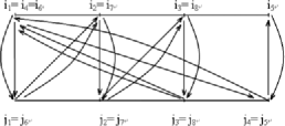
Figure 1: An example of W-graph.

Two graphs are said to be isomorphic if one becomes another by an appropriate permutation on $\{1,2,\ldots,p\}$ of I-vertices and an appropriate permutation on $\{1,2,\ldots,n\}$ of J-vertices. A W-graph is called a canonical graph if $i_{a}\leq\max\{i_{1},i_{2},\ldots,i_{a-1}\}+1$ and $j_{a}\leq\max\{j_{1},j_{2},\ldots,j_{a-1}\}+1$ with $i_{1}=j_{1}=1$, where $a=1,2,\ldots,k$.

In the canonical graph, if $i_{a+1}=\max\{i_{1},i_{2},\ldots,i_{a}\}+1$, then the edge $j_{a}i_{a+1}$ is called a row innovation and if $j_{a}=\max\{j_{1},j_{2},\ldots,j_{a-1}\}+1$, then the edge $i_{a}j_{a}$ is called a column innovation. Apparently, a row innovation and a column innovation, respectively, lead to a new I-vertex and a new J-vertex except the first column innovation $i_{1}j_{1}$ leading to a new I-vertex $i_{1}$ and a new J-vertex $j_{1}$.

We now classify all edges into three types, $T_{1}$, $T_{3}$ and $T_{4}$. Let $T_{1}$ denote the set of all innovations including row innovations and column innovations. We further distinguish the column innovations as follows. An edge $i_{a}j_{a}$ is called a $T_{11}$ edge if it is a column innovation and the edge $j_{a}i_{a+1}$ is a row innovation; An edge $i_{b}j_{b}$ is referred to as a $T_{12}$ edge if it is a column innovation but $j_{b}i_{b+1}$ is not a row innovation. An edge $e_{j}$ is said to be a $T_{3}$ edge if there is an innovation edge $e_{i},i<j$ so that $e_{j}$ is the first one to coincide with $e_{i}$. An edge is called a $T_{4}$ edge if it does not belong to a $T_{1}$ edge or $T_{3}$ edge. The first appearance of a $T_{4}$ edge is referred to as a $T_{2}$ edge. There are two kinds of $T_{2}$ edges: (a) the first appearance of an edge that coincides with a $T_{3}$ edge, denoted by $T_{21}$ edge; (b) the first appearance of an edge that is not an innovation, denoted by $T_{22}$ edge.

We say that an edge $e_{i}$ is single up to the edge $e_{j},j\geq i$, if it does not coincide with any other edges among $e_{1},\ldots,e_{j}$ except itself. A $T_{3}$ edge $e_{i}$ is said to be regular if there are more than one innovations with a vertex equal to the initial vertex of $e_{i}$ and single up to $e_{i-1}$, among the edges $\{e_{1},\ldots,e_{i-1}\}$. All other $T_{3}$ edges are called irregular $T_{3}$ edges.

Corresponding to the above classification of the edges, we introduce the following notation and list some useful facts.

1. [6.]

2. Denote by $l$ the total number of innovations.

3. Let $r$ be the number of the row innovations. Moreover, let $c$ denote the column innovations. We then have $r+c=l$.

4. Define $r_{1}$ to be the number of the $T_{11}$ edges. Then $r_{1}\leq r$ by the definition of a $T_{11}$ edge. Also, the number of the $T_{12}$ edges is $l-r-r_{1}$.

5. Let $t$ be the number of the $T_{2}$ edges. Note that the number of the $T_{3}$ edges is the same as the number of the innovations and there are a total of $2k$ edges in the graph. It follows that the number of the $T_{4}$ edges is $2k-2l$. On the other hand, each $T_{2}$ edge is also a $T_{4}$ edge. Therefore, $t\leq 2k-2l$.

6. Define $\mu$ to be the number of $T_{21}$ edges. Obviously, $\mu\leq t$. The number of $T_{22}$ edge is then $t-\mu$. Since each $T_{21}$ edge coincides with one innovation, we let $n_{i},i=1,2,\ldots,\mu$, denote the number of $T_{4}$ edges which coincide with the $i$th such innovation, $n_{i}\geq 0$.

7. Let $\mu_{1}$ be the number of $T_{21}$ edges which do not coincide with the other $T_{4}$ edges. That is $\mu_{1}=\#\{i\colon\ n_{i}=1,i=1,2,\ldots,\mu\}$, where $\#\{\cdot\}$ denotes the cardinality of the set $\{\cdot\}$.

8. Let $m_{j},j=1,2,\ldots,t-\mu$, denote the number of $T_{4}$ edges which coincide with and include the $j$th $T_{22}$ edge. Note that $m_{j}\geq 2$.

We now claim that

$$Etr(B_{p}^{k}) \leq \bigl{(}2\sqrt{np}\bigr{)}^{-k}\sum E(X_{i_{1}j_{1}}X_{i_{2}j_{1}}\cdots X_{i_{k}j_{k}}X_{i_{1}j_{k}})$$

$$= \bigl{(}2\sqrt{np}\bigr{)}^{-k}\sum{{}^{\prime}}\sum{{}^{\prime\prime}}\sum{{}^{\prime\prime\prime}}\sum_{*}E(X_{i_{1}j_{1}}X_{i_{2}j_{1}}\cdots X_{i_{k}j_{k}}X_{i_{1}j_{k}})$$

$$\leq \bigl{(}2\sqrt{np}\bigr{)}^{-k}\sum_{l=1}^{k}\sum_{r=1}^{l}\sum_{r_{1}=0}^{r}\sum_{t=0}^{2k-2l}\sum_{\mu=0}^{t}\sum_{\mu_{1}=0}^{\mu}\sum_{*}\pmatrix{k\cr r}\pmatrix{r\cr r_{1}}\pmatrix{k-r_{1}\cr l-r-r_{1}}\pmatrix{2k-l\cr l}$$

$${}\times k^{3t}(t+1)^{6k-6l}\bigl{(}\delta\sqrt[4]{np}\bigr{)}^{2k-2l-2t+\mu_{1}}p^{r+1}n^{l-r},$$

where the summation $\sum{{}^{\prime}}$ is with respect to different arrangements of three types of edges at the $2k$ different positions, the summation $\sum{{}^{\prime\prime}}$ over different canonical graphs with a given arrangement of the three types of edges for $2k$ positions, the third summation $\sum{{}^{\prime\prime\prime}}$ with respect to all isomorphic graphs for a given canonical graph and the last notation $\sum_{*}$ denotes the constraint that $i_{1}\neq i_{2},i_{2}\neq i_{3},\ldots,i_{k}\neq i_{1}$.

Now, we explain why the above estimate is true:

1. [(viii)]

2. The factor $(2\sqrt{np})^{-k}$ is obvious.

3. If the graph is not a W-graph, which means there is a single edge in the graph, then the mean of the product of $X_{ij}$ corresponding to this graph is zero (since $EX_{11}=0$). Thus, we have $l\leq k$. Moreover, the facts that $r\leq l$, $r_{1}\leq r$, $t\leq 2k-2l$, $\mu\leq t$ and $\mu_{1}\leq\mu$ are easily obtained from the fact $1$ to the fact $7$ listed before.

4. There are at most ${k\choose r}$ ways to choose $r$ edges out of the $k$ row edges to be the $r$ row innovations. Subsequently, we consider how to select the column innovations. Observe that the definition of $T_{11}$ edges, there are ${r\choose r_{1}}$ ways to select $r_{1}$ row innovations out of the total $r$ row innovations so that the edge before each such $r_{1}$ row innovations is a $T_{11}$ edge, column innovation. Moreover, there are at most ${k-r_{1}\choose l-r-r_{1}}$ ways to choose $l-r-r_{1}$ edges out of the remaining $k-r_{1}$ column edges to be the $l-r-r_{1}$ $T_{12}$ edges, the remaining column innovations.

5. Given the position of the $l$ innovations, there are at most ${2k-l\choose l}$ ways to select $l$ edges out of the $2k-l$ edges to be $T_{3}$ edges. And the rest positions are for the $T_{4}$ edges. Therefore, the first summation $\sum{{}^{\prime}}$ is bounded by $\sum_{l=1}^{k}\sum_{r=1}^{l}\sum_{r_{1}=0}^{r}{k\choose r}{r\choose r_{1}}{k-r_{1}\choose l-r-r_{1}}{2k-l\choose l}$.

6. By definition, each innovation (or each irregular $T_{3}$ edges) is uniquely determined by the subgraph prior to the innovation (or the irregular $T_{3}$). Moreover, by Lemma 3.2 in [11] for each regular $T_{3}$ edge, there are at most $t+1$ innovations so that the regular $T_{3}$ edge coincides with one of them and by Lemma 3.3 in [11] there are at most $2t$ regular $T_{3}$ edges. Therefore, there are at most $(t+1)^{2t}\leq(t+1)^{2(2k-2l)}$ ways to draw the regular $T_{3}$ edges.

7. Once the positions of the innovations and the $T_{3}$ edges are fixed there are at most ${(r+1)c\choose t}\leq{k^{2}\choose t}\leq k^{2t}$ ways to arrange the $t$ $T_{2}$ edges, as there are $r+1$ I-vertices and $c$ J-vertices. After $t$ positions of $T_{2}$ edges are determined there are at most $t^{2k-2l}$ ways to distribute $2k-2l$ $T_{4}$ edges among the $t$ positions. So there are at most $k^{2t}\cdot t^{2k-2l}$ ways to arrange $T_{4}$ edges. It follows that $\sum{{}^{\prime\prime}}$ is bounded by $\sum_{t=0}^{2k-2l}(t+1)^{2(2k-2l)}k^{2t}\cdot t^{2k-2l}$.

8. The third summation $\sum{{}^{\prime\prime\prime}}$ is bounded by $n^{c}p^{r+1}$ because the number of graphs in the isomorphic class for a given graph is $p(p-1)\cdots(p-r)n(n-1)\cdots(n-c+1)$.

9. Recalling the definitions of $l,r,t,\mu,\mu_{1},n_{i},m_{i}$, we have

   $$EX_{i_{1}j_{1}}X_{i_{2}j_{1}}\cdots X_{i_{k}j_{k}}X_{i_{1}j_{k}}=(EX_{11}^{2})^{l-\mu}\Biggl{(}\prod_{i=1}^{\mu}EX_{11}^{n_{i}+2}\Biggr{)}\Biggl{(}\prod_{i=1}^{t-\mu}EX_{11}^{m_{i}}\Biggr{)},$$ (14)

   where $\sum_{i=1}^{\mu}n_{i}+\sum_{i=1}^{t-\mu}m_{i}=2k-2l$. Without loss of generality, we suppose $n_{1}=n_{2}=\cdots=n_{\mu_{1}}=1$ and $n_{\mu_{1}+1},\ldots,n_{\mu}\geq 2$ for convenience. It is easy to check that

   $$E|X_{11}^{s}|\leq\left\{\begin{array}[]{l@{ \qquad}l}M\bigl{(}\delta\sqrt[4]{np}\bigr{)}^{s-4},&\mbox{if }s\geq 4,M=\operatorname{max}\{EX_{11}^{4},|EX_{11}^{3}|\},\\ \bigl{(}\delta\sqrt[4]{np}\bigr{)}^{s-2},&\mbox{if }s\geq 2.\end{array}\right.$$

   Thus, (14) becomes

   $$|EX_{i_{1}j_{1}}X_{i_{2}j_{1}}\cdots X_{i_{k}j_{k}}X_{i_{1}j_{k}}|$$

   $$\quad\leq\sum_{\mu=0}^{t}\sum_{\mu_{1}=0}^{\mu}|EX_{11}^{3}|^{\mu_{1}}|EX_{11}^{4}|^{t-\mu_{1}}\bigl{(}\delta\sqrt[4]{np}\bigr{)}^{\sum_{i=\mu_{1}+1}^{\mu}n_{i}-2(\mu-\mu_{1})}\bigl{(}\delta\sqrt[4]{np}\bigr{)}^{\sum_{i=1}^{t-\mu}m_{i}-2(t-\mu)}$$

   (16)

   $$\quad\leq\sum_{\mu=0}^{t}\sum_{\mu_{1}=0}^{\mu}M^{t}\bigl{(}\delta\sqrt[4]{np}\bigr{)}^{2k-2l-2t+\mu_{1}}$$

   $$\quad\leq\sum_{\mu=0}^{t}\sum_{\mu_{1}=0}^{\mu}k^{t}\bigl{(}\delta\sqrt[4]{np}\bigr{)}^{2k-2l-2t+\mu_{1}},\qquad\mbox{when $k$ is large enough}.$$

The above points regarding the $T_{2}$ edges are discussed for $t>0$, but they are still valid when $t=0$ with the convention that $0^{0}=1$ in the term $t^{2k-2l}$, because in this case there are only $T_{1}$ edges and $T_{3}$ edges in the graph and thus $l=k$.

Consider the constraint $\sum_{*}$ now. Note that for each $T_{12}$ edge, say $i_{a}j_{a}$, it is a column innovation, but the next row edge $j_{a}i_{a+1}$ is not a row innovation. Since $i_{a+1}\neq i_{a}$, the edge $j_{a}i_{a+1}$ cannot coincide with the edge $i_{a}j_{a}$. Moreover, it also doesn’t coincide with any edges before the edge $i_{a}j_{a}$ since $j_{a}$ is a new vertex. So $j_{a}i_{a+1}$ must be a $T_{22}$ edge. Thus, the number of the $T_{12}$ edges cannot exceed the number of the $T_{22}$ edges. This implies $l-r-r_{1}\leq t-\mu$. Moreover, note that $\mu_{1}\leq\mu$. We then have

$$n^{-k/2}p^{-k/2}n^{l-r}p^{r+1}(np)^{k/2-l/2-t/2+\mu_{1}/4}$$

$$\quad=(n/p)^{l/2}\cdot n^{-r-t/2+\mu_{1}/4}p^{r+1-t/2+\mu_{1}/4}$$ (17)

$$\quad\leq\Biggl{(}\sqrt{\frac{p}{n}}\Biggr{)}^{r-r_{1}}\cdot p^{-t/2}p.$$

We thus conclude from (3) and (3) that

$$Etr(B_{p}^{k}) \leq 2^{-k}\sum_{l=1}^{k}\sum_{r=1}^{l}\sum_{r_{1}=0}^{r}\sum_{t=0}^{2k-2l}\sum_{\mu=0}^{t}\sum_{\mu_{1}=0}^{\mu}\pmatrix{k\cr r}\pmatrix{r\cr r_{1}}\pmatrix{k-r_{1}\cr l-r-r_{1}}\pmatrix{2k-l\cr l}$$

$${}\times\Biggl{(}\sqrt{\frac{p}{n}}\Biggr{)}^{r-r_{1}}p^{-t/2}pk^{3t}(t+1)^{6k-6l}\delta^{2k-2l-2t+\mu_{1}}.$$

Moreover, we claim that

$$p\biggl{[}2^{-k}\pmatrix{k\cr r}\biggr{]}\Biggl{[}\pmatrix{r\cr r_{1}}\Biggl{(}\sqrt{\frac{p}{n}}\Biggr{)}^{r-r_{1}}\Biggr{]}\biggl{[}\pmatrix{k-r_{1}\cr l-r-r_{1}}\delta^{l-r-r_{1}}\biggr{]}$$

$$\quad{}\times\biggl{[}\pmatrix{2k-l\cr l}\biggl{(}\frac{\sqrt{p}\delta^{3}}{k^{3}}\biggr{)}^{-t}(t+1)^{6k-6l}\delta^{2k-2l}\biggr{]}\delta^{-(l-r-r_{1})+3t-(2k-2l)}\cdot\delta^{2k-2l-2t+\mu_{1}}$$ (19)

$$\quad\leq p^{2}\Biggl{(}1+\sqrt{\frac{p}{n}}\Biggr{)}^{k}(1+\delta)^{k}\biggl{(}1+\frac{24^{3}k^{3}\delta}{\log^{3}{p}}\biggr{)}^{2k}.$$

Indeed, the above claim is based on the following five facts. (

• 5)]

• $2^{-k}{k\choose r}\leq 2^{-k}\mathop{\sum}_{r=0}^{k}{k\choose r}=1$.

• ${r\choose r_{1}}(\sqrt{\frac{p}{n}})^{r-r_{1}}={r\choose r-r_{1}}(\sqrt{\frac{p}{n}})^{r-r_{1}}\leq\mathop{\sum}_{s=0}^{r}{r\choose s}(\sqrt{\frac{p}{n}})^{s}=(1+\sqrt{\frac{p}{n}})^{r}\leq(1+\sqrt{\frac{p}{n}})^{k}$.

• ${k-r_{1}\choose l-r-r_{1}}\delta^{l-r-r_{1}}\leq\mathop{\sum}_{s=0}^{k-r_{1}}{k-r_{1}\choose s}\delta^{s}=(1+\delta)^{k-r_{1}}\leq(1+\delta)^{k}$.

• By the fact that ${2k-l\choose l}\leq{2k\choose 2l}$, and the inequality $a^{-t}(t+1)^{b}\leq a(\frac{b}{\log{a}})^{b}$, for $a>1$, $b>0$, $t>0$ and $\frac{\delta^{2}\sqrt{p}}{k^{3}}\geq\sqrt[4]{p}$, we have

  $$\pmatrix{2k-l\cr l}\biggl{(}\frac{\sqrt{p}\delta^{3}}{k^{3}}\biggr{)}^{-t}(t+1)^{6k-6l}\delta^{2k-2l} \leq \pmatrix{2k\cr 2l}\frac{\sqrt{p}\delta^{3}}{k^{3}}\biggl{(}\frac{6k-6l}{\log{(\sqrt{p}\delta^{3}/k^{3})}}\biggr{)}^{6k-6l}\delta^{2k-2l}$$

  $$\leq p\pmatrix{2k\cr 2l}\biggl{(}\frac{24k}{\log{p}}\biggr{)}^{6k-6l}\delta^{2k-2l}$$

  $$\leq p\pmatrix{2k\cr 2l}\biggl{(}\frac{24^{3}k^{3}\delta}{\log^{3}{p}}\biggr{)}^{2k-2l}$$

  $$\leq p\sum_{s=0}^{2k}\pmatrix{2k\cr s}\biggl{(}\frac{24^{3}k^{3}\delta}{\log^{3}{p}}\biggr{)}^{2k-s}$$

  $$= p\biggl{(}1+\frac{24^{3}k^{3}\delta}{\log^{3}{p}}\biggr{)}^{2k}.$$

• When $p$ is large enough, $\delta^{-(l-r-r_{1})+3t-(2k-2l)}\cdot\delta^{2k-2l-2t+\mu_{1}}=\delta^{t-(l-r-r_{1})}\cdot\delta^{\mu_{1}}\leq 1$, since $\delta\to 0$ and $l-r-r_{1}\leq t-\mu$.

Summarizing (3) and (3), we obtain that

$$Etr(B_{p}^{k}) \leq \sum_{l=1}^{k}\sum_{r=1}^{l}\sum_{r_{1}=0}^{r}\sum_{t=0}^{2k-2l}\sum_{\mu=0}^{t}\sum_{\mu_{1}=0}^{\mu}p^{2}\Biggl{(}1+\sqrt{\frac{p}{n}}\Biggr{)}^{k}(1+\delta)^{k}\biggl{(}1+\frac{24^{3}l^{3}\delta}{\log^{3}{p}}\biggr{)}^{2k}$$

$$\leq 8k^{6}p^{2}\Biggl{(}1+\sqrt{\frac{p}{n}}\Biggr{)}^{k}(1+\delta)^{k}\biggl{(}1+\frac{24^{3}l^{3}\delta}{\log^{3}{p}}\biggr{)}^{2k}$$

$$= \Biggl{(}(8k^{6})^{1/k}p^{2/k}\Biggl{(}1+\sqrt{\frac{p}{n}}\Biggr{)}(1+\delta)\biggl{(}1+\frac{24^{3}k^{3}\delta}{\log^{3}{p}}\biggr{)}^{2}\Biggr{)}^{k}$$

$$\leq \eta^{k},$$

where $\eta$ is a constant satisfying $1<\eta<1+\epsilon$. Here the last inequality uses the facts below:

1. [(iii)]

2. $(p^{2})^{1/k}\to 1$, because $k/\log{p}\to\infty$,

3. $(8k^{6})^{1/k}\to 1$, because $k\to\infty$,

4. $(1+\sqrt{\frac{p}{n}})\to 1$, because $p/n\to 0$,

5. $(1+\delta)\to 1$, because $\delta\to 0$,

6. $\frac{24^{3}\cdot k^{3}\delta}{\log^{3}{p}}\to 0$, because $\frac{\delta^{1/3}k}{\log{p}}\to 0.$

It follows that

$$P\bigl{(}\lambda_{\mathrm{max}}({\mathbf{B}}_{p})>1+\epsilon\bigr{)}\leq\biggl{(}\frac{\eta}{1+\epsilon}\biggr{)}^{k}=\mathrm{o}(p^{-\ell})$$

since $k/\log{p}\to\infty$ and $\frac{\eta}{1+\epsilon}<1$. The proof is complete.

4 Proof of Theorem 3

Note that

$${\mathbf{S}}_{1}={\mathbf{S}}-\bar{\mathbf{s}}\bar{\mathbf{s}}^{\prime}.$$ (20)

By the Fan inequality [6],

$$\sup_{x}|F^{{\mathbf{A}}_{p1}}(x)-F^{{\mathbf{A}}_{p}}(x)|\leq\frac{1}{p}.$$

Thus from theorem in [2], we see that

$$F^{{\mathbf{A}}_{p1}}(x)\stackrel{{\scriptstyle\mathrm{a.s.}}}{{\longrightarrow}}F(x),$$

specified in the introduction. It follows that

$$\liminf_{p\rightarrow\infty}\lambda_{\max}({\mathbf{A}}_{p1})\geq 1.$$

Let ${\mathbf{z}}$ be a unit vector. In view of (20), we obtain

$${\mathbf{z}}^{\prime}{\mathbf{A}}_{p1}{\mathbf{z}}={\mathbf{z}}^{\prime}{\mathbf{A}}_{p}{\mathbf{z}}-\frac{1}{2}\sqrt{\frac{n}{p}}{\mathbf{z}}^{\prime}\bar{\mathbf{s}}\bar{\mathbf{s}}^{\prime}{\mathbf{z}}\leq{\mathbf{z}}^{\prime}{\mathbf{A}}_{p}{\mathbf{z}},$$

which implies that

$$\lambda_{\max}({\mathbf{A}}_{p1})\leq\lambda_{\max}({\mathbf{A}}_{p}).$$

This, together with Theorem 1, finishes the proof of Theorem 3.

5 Proof of Theorem 4

Theorem 4 follows from Theorem 3 and the fact that

$$\|{\mathbf{S}}_{2}-\Sigma\|=\|\Sigma^{1/2}({\mathbf{S}}_{1}-{\mathbf{I}}_{p})\Sigma^{1/2}\|\leq\|{\mathbf{S}}_{1}-{\mathbf{I}}_{p}\|\|\Sigma\|.$$

References

• [1] {barticle}[mr] \bauthor\bsnmAdamczak,Β \bfnmRadosΕ‚aw\binitsR., \bauthor\bsnmLitvak,Β \bfnmAlexanderΒ E.\binitsA.E., \bauthor\bsnmPajor,Β \bfnmAlain\binitsA. &\bauthor\bsnmTomczak-Jaegermann,Β \bfnmNicole\binitsN. (\byear2010). \btitleQuantitative estimates of the convergence of the empirical covariance matrix in log-concave ensembles. \bjournalJ. Amer. Math. Soc. \bvolume23 \bpages535–561. \biddoi=10.1090/S0894-0347-09-00650-X, issn=0894-0347, mr=2601042 \bptokimsref \endbibitem
• [2] {barticle}[mr] \bauthor\bsnmBai,Β \bfnmZ.Β D.\binitsZ.D. &\bauthor\bsnmYin,Β \bfnmY.Β Q.\binitsY.Q. (\byear1988). \btitleConvergence to the semicircle law. \bjournalAnn. Probab. \bvolume16 \bpages863–875. \bidissn=0091-1798, mr=0929083 \bptokimsref \endbibitem
• [3] {barticle}[mr] \bauthor\bsnmBai,Β \bfnmZ.Β D.\binitsZ.D. &\bauthor\bsnmYin,Β \bfnmY.Β Q.\binitsY.Q. (\byear1993). \btitleLimit of the smallest eigenvalue of a large-dimensional sample covariance matrix. \bjournalAnn. Probab. \bvolume21 \bpages1275–1294. \bidissn=0091-1798, mr=1235416 \bptokimsref \endbibitem
• [4] {barticle}[mr] \bauthor\bsnmElΒ Karoui,Β \bfnmNoureddine\binitsN. (\byear2008). \btitleOperator norm consistent estimation of large-dimensional sparse covariance matrices. \bjournalAnn. Statist. \bvolume36 \bpages2717–2756. \biddoi=10.1214/07-AOS559, issn=0090-5364, mr=2485011 \bptokimsref \endbibitem
• [5] {bmisc}[auto:STBβ€”2011/10/28β€”06:47:38] \bauthor\bsnmEl Karoui,Β \bfnmN.\binitsN. (\byear2003). \bhowpublishedOn the largest eigenvalue of Wishart matrices with identity covariance when $n$, $p$ and $p/n$ tend to infinity. Preprint. \bptokimsref \endbibitem
• [6] {barticle}[mr] \bauthor\bsnmFan,Β \bfnmKy\binitsK. (\byear1951). \btitleMaximum properties and inequalities for the eigenvalues of completely continuous operators. \bjournalProc. Natl. Acad. Sci. USA \bvolume37 \bpages760–766. \bidissn=0027-8424, mr=0045952 \bptokimsref \endbibitem
• [7] {barticle}[mr] \bauthor\bsnmGeman,Β \bfnmStuart\binitsS. (\byear1980). \btitleA limit theorem for the norm of random matrices. \bjournalAnn. Probab. \bvolume8 \bpages252–261. \bidissn=0091-1798, mr=0566592 \bptokimsref \endbibitem
• [8] {barticle}[mr] \bauthor\bsnmJonsson,Β \bfnmDag\binitsD. (\byear1982). \btitleSome limit theorems for the eigenvalues of a sample covariance matrix. \bjournalJ. Multivariate Anal. \bvolume12 \bpages1–38. \biddoi=10.1016/0047-259X(82)90080-X, issn=0047-259X, mr=0650926 \bptokimsref \endbibitem
• [9] {barticle}[auto:STBβ€”2011/10/28β€”06:47:38] \bauthor\bsnmMarčenko,Β \bfnmV.Β A.\binitsV.A. &\bauthor\bsnmPastur,Β \bfnmL.Β A.\binitsL.A. (\byear1967). \btitleDistribution for some sets of random matrices. \bjournalMath. USSR-Sb. \bvolume1 \bpages457–483. \bptokimsref \endbibitem
• [10] {barticle}[mr] \bauthor\bsnmWigner,Β \bfnmEugeneΒ P.\binitsE.P. (\byear1958). \btitleOn the distribution of the roots of certain symmetric matrices. \bjournalAnn. of Math. (2) \bvolume67 \bpages325–327. \bidissn=0003-486X, mr=0095527 \bptokimsref \endbibitem
• [11] {barticle}[mr] \bauthor\bsnmYin,Β \bfnmY.Β Q.\binitsY.Q., \bauthor\bsnmBai,Β \bfnmZ.Β D.\binitsZ.D. &\bauthor\bsnmKrishnaiah,Β \bfnmP.Β R.\binitsP.R. (\byear1988). \btitleOn the limit of the largest eigenvalue of the large-dimensional sample covariance matrix. \bjournalProbab. Theory Related Fields \bvolume78 \bpages509–521. \biddoi=10.1007/BF00353874, issn=0178-8051, mr=0950344 \bptokimsref \endbibitem