Geometrical approach to separation of variables
in mechanical systems

Abstract.

The article presents a compact review of the analytical results (2002–2009) in the study of the system describing the motion of a top in two constant fields. The Liouville integrability of this system under certain condition of the Kowalevski type was established by A.G. Reyman and M.A. Semenov-Tian-Shansky. We present some geometrical foundations of finding separations of variables. Two systems of local planar coordinates are introduced leading to separation of variables for two subsystems with two degrees of freedom in the dynamics of the generalized Kowalevski top.

1. Introduction

Historically, the main goal in the study of a differential equation of mechanics was to integrate it, to find the explicit solution. The fact of the existence of principally non-integrable systems has shifted the accent to qualitative methods of investigation. However, during the last 20 years new algebraic approaches to construct or reveal the integrable systems were created. For Hamiltonian systems, many new cases of commutative and non-commutative integrability were found. A lot of them deal with the problem of the rotation of a rigid body about a fixed point and its generalizations to Lie groups that differ from $SO(3)$. Here lies one of the reasons for a new wave of mathematical interest in the integrable Hamiltonian systems. Note the books [1, 2, 3, 4, 5] published lately and containing more than a thousand of references on the matter. In relatively recent studies, the integrable systems with three or more degrees of freedom were found not having continuous symmetries and therefore not reducible as a whole to families of systems with two degrees of freedom (the so-called irreducible systems). One of the most ingenious and complicated example of the integrable irreducible system is the generalized Kowalevski gyrostat. It is a rigid body with a rotor satisfying the conditions of the Kowalevski type and placed in two independent constant fields, say, gravitational and magnetic. This case was found due to the efforts of several mathematicians. We note the works of O.I. Bogoyavlensky [6, 7, 8], H.M. Yehia [9, 10], L.N. Gavrilov [11], I.V. Komarov [12]. The final and mostly general result was obtained by A.G. Reyman and M.A. Semenov-Tian-Shansky [13, 14]. Nevertheless, it appeared that no explicit solutions in the classical sense can be found for the general case. Up-to-date the only progress in studying the Reyman–Semenov-Tian-Shansky case is based on the idea of investigating critical subsystems. This row of publications starts from the work [15], in which the Bogoyavlensky system generalizing the 1st Appelrot class is investigated without any connection to the general case, and the work [16], in which the next generalization, of the 2nd and 3d Appelrot classes, was found. Later, the bifurcation diagrams of the partial cases and of the general case including the case of a gyrostat were built and classified in the space of parameters and with respect to the energy levels in the series of works [17, 18, 19, 20, 21, 22, 23]. The complete description was obtained for the critical set of the momentum mapping stratified according to various criteria [24]. For two critical subsystems generalizing the famous Appelrot classes separations of variables were found and the phase topology was investigated in [25, 26, 27, 28, 29, 30], all critical periodic motions were described analytically and integrated in elliptic functions for the cases of a top [31, 18] and of a gyrostat [32, 33]. From the integrability point of view, each of the critical subsystems found is as general as the whole Kowalevski case in the gravity field, i.e., generates a one-parametric family of Hamiltonian systems with two degrees of freedom. These systems have all the features of the systems in which separation of variables is obtained algebraically. Here we call such systems algebraically solvable. We present though the geometrical ideas of how to construct such separations.

A lot of publications deal with the notion of an algebraic complete integrable systems. This notion does not have a unique and exact definition. Usually it is associated with Hamiltonian systems the topology of which is connected with the Jacobians and Prim varieties of algebraic surfaces. Algebraic complete integrable systems with known separation of variables usually also have algebraic expressions of the initial phase variables in terms of the separated ones, although many contemporary papers, not like the classical works, do not pay much attention to this point. We think that a system with separated variables cannot be considered completely analytically integrated without explicit expressions for the phase variables. Separations of variables on algebraic curves generated by Lax representations, the existence of which is theoretically proved, do not provide any method to establish the connection with the initial variables. Here we use another approach — starting from the geometry of initial variables and trying to find such projections of the phase space which bring the integral manifolds to the most simple image. If it is done (and there are no general ways to do it), then the connection with the initial variables is kept from the beginning. In this paper we propose the projections and the coordinate systems that made it possible to find new algebraically and topologically interesting separations of variables. The examples given below show the valuable applications.

2. Geometrical approach to separation of variables

2.1. Geometry of separated variables

The term we use here—algebraically solvable systems—is not a standard one. Let us give some explanations of the problem. Consider a system of differential equations on a submanifold $\mathcal{P}$ in a real vector space

$$\frac{d\mathbf{x}}{dt}=\mathbf{X}(\mathbf{x}),\quad\mathbf{x}\in\mathcal{P}\subset V$$ (2.1)

defining the evolution of the set of phase variables ${\mathbf{x}}$ and admitting separation of variables

$$\frac{ds_{i}}{d\tau}=\sqrt{\vphantom{\bigl{(}}P_{i}(s_{i};\mathbf{f})},$$ (2.2)

where $s_{i}$ are so-called auxiliary or separated variables. We denote the vector of these variables by $\mathbf{s}$. The functions $P_{i}(s;\mathbf{f})$ are supposed to be polynomials in one variable $s$ with coefficients depending on a set of arbitrary constants ${\mathbf{f}}$, $\tau$ is the “reduced time” connected with the real time $t$ by the equation of the type $d\tau/dt=\rho(\mathbf{s})>0$. Usually such separation has a mechanical origin, therefore equations (2.2) have the form of an energy integral. Moreover, we suppose that all phase variables $x_{j}$ are expressed via the separated variables by rational functions with respect to the set of radicals

$$R_{i\alpha}=\sqrt{\vphantom{\bigl{(}}s_{i}-e_{\alpha}}\quad\quad(e_{\alpha}\in{\mathbf{C}})$$

with coefficients smoothly depending on $\mathbf{s}$. The set of numbers $\{e_{\alpha}\}$ depending, of course, on the constants ${\mathbf{f}}$ includes also the roots of $P_{i}$. The classical examples show that the roots of $P_{i}$ usually provide the whole set of $\{e_{\alpha}\}$.

The vector ${\mathbf{f}}$ for the system (2.1) usually appears as a collection of arbitrary constants of some set of first integrals $\{{\mathcal{F}}_{j}\}$. The dependencies

$${\mathbf{x}}={\mathbf{x}}({\mathbf{s}};{\mathbf{f}}),\quad{\mathbf{s}}\in\mathop{\rm Acc}\nolimits({\mathbf{f}})$$ (2.3)

then are considered as the multi-valued parametric equations of an integral manifold $\mathcal{F}_{\mathbf{f}}\doteq{\mathcal{F}}^{-1}({\mathbf{f}})\subset{\mathcal{P}}$. Here $\mathop{\rm Acc}\nolimits({\mathbf{f}})$ is the region in the separated variables space filled with trajectories of (2.2) for given ${\mathbf{f}}$. In Russian, it is traditionally called by the term corresponding to “the region of the possibility of motions” [34, 35], which sounds not very elegant. A shorter term “accessible region” was introduced in English translations and completely reflects the situation. Notation of the region $\mathop{\rm Acc}\nolimits({\mathbf{f}})$ for the argument vector $\mathbf{s}$ in (2.3) is based on this term.

Let the system (2.1) be a Hamiltonian complete integrable system with two degrees of freedom and

$$\mathcal{F}:\mathcal{P}\to{\mathbf{R}}^{2}$$ (2.4)

be its integral mapping of compact character (the inverse image of a compact set is compact). Two degrees of freedom are chosen to simplify notation and because of the main examples below.

Definition 1.

The set $\operatorname{Im}\mathcal{F}$ is called the admissible region ${\rm(}$in the space of integral constants${\rm)}.$ A point ${\mathbf{f}}\in{\mathbf{R}}^{2}$ is called an admissible point if and only if ${\mathcal{F}^{-1}(\mathbf{f})\neq\varnothing}$.

Generally speaking, separation of variables is some mapping

$$\pi:\mathcal{P}\to{\mathbf{R}}^{2}_{(s_{1},s_{2})}$$ (2.5)

of the phase space to the plane of the auxiliary variables $(s_{1},s_{2})$ that takes the system (2.1) to the system (2.2) with $i=1,2$. For any admissible ${\mathbf{f}}$ we obtain the mapping

$$\pi_{\mathbf{f}}:\mathcal{F}_{\mathbf{f}}\to{\mathbf{R}}^{2}_{(s_{1},s_{2})}.$$ (2.6)

Definition 2.

For a given ${\mathbf{f}}$ the set $\mathop{\rm Acc}\nolimits({\mathbf{f}})=\pi_{\mathbf{f}}(\mathcal{F}_{\mathbf{f}})$ is called an accessible region in the plane of the separated variables.

It is clear that $\mathop{\rm Acc}\nolimits({\mathbf{f}})$ is a subset of

$$\{(s_{1},s_{2}):P_{i}(s_{i},{\mathbf{f}})\geqslant 0,i=1,2\},$$ (2.7)

and any point is included in $\mathop{\rm Acc}\nolimits({\mathbf{f}})$ with its total connected component in the set (2.7). Then $\mathop{\rm Acc}\nolimits({\mathbf{f}})$ is a collection of rectangular regions in the $(s_{1},s_{2})$-plane; “infinite rectangles” (half-strips, strips or even quadrants) are also possible. The fact that the accessible region is rectangular for all integral constants, obviously, is the necessary condition of separation of variables. Possibly, supposing that the projection of the type (2.6) is non-trivial in some sense or that the boundaries of accessible regions essentially depend on $\mathbf{f}$ in terms of the corresponding Jacobians, one can prove that this fact is also sufficient, but here we do not consider such a goal. We want to understand in which way to look for separations of variables.

Note that separation of variables not always has the form of a global mapping (2.5). As far as the dynamics of a rigid body is concerned, separations not depending on integral constants are known for the Euler case (one independent variable can also be treated as a separation), the Goryachev–Chaplygin case and its generalization to a gyrostat given by L.N. Sretensky [36], the Clebsch case with zero momentum constant (isomorphic to the Neumann problem). Already in the Kowalevski case [37], the change of variables leading to separation essentially uses the integral equations. However, having the mapping (2.6) for all $\mathbf{f}$ one can formally substitute $\mathbf{f}=\mathcal{F}(\mathbf{x})$ to obtain some mapping of the type (2.5). It is important to mention that practically in all cases separation of variables is not built straightforwardly in the form (2.5). As a rule, some intermediate mapping $\mathcal{P}\to\mathbf{R}^{2}_{\boldsymbol{\xi}}$ is constructed first. Let us call this auxiliary plane of the variables $\xi_{1},\xi_{2}$ the picture plane. With the projection onto the picture plane, the separated variables are introduced as the functions of $\xi_{1},\xi_{2},\mathbf{f}$ (usually defined by some implicit equations).

What is the geometry behind this construction? The mapping of the phase space to the picture plane takes an integral manifold to a region $\mathcal{F}_{\mathbf{f}}$ bounded by some curves. If these curves could be included in a two-parametric family of curves on the plane $\mathbf{R}^{2}_{\boldsymbol{\xi}}$ and this family could serve as a local coordinate net, then in these coordinates the image of each integral manifold would be a rectangle. Therefore, the new coordinates satisfy the necessary condition of a separation and we obtain hope to build such a separation. At this moment it absolutely does not matter whether this coordinate net was built by a global change of variables or, as in the Kowalevski case, this net (the Zhukovsky net) depends in a very complicated way on the integral constants.

Studying the projections of $\mathcal{P}$ onto the picture plane (or in more general case onto some picture manifold with dimension equal to the number of degrees of freedom) we must have in mind that $\mathcal{P}$ itself may not have a global coordinate system. For example, in the rigid body dynamics $\mathcal{P}=\mathbf{R}^{3}{\times}SO(3)$ with the matrix group $SO(3)$ naturally embedded in $\mathbf{R}^{9}$ by means of the so-called direction cosines. Any system of three coordinates either not covers $SO(3)$ or has inevitable singularities (like the Euler angles or their modifications). It is one of the reasons to consider $\mathcal{P}$ as a subset in a vector space $V$ of sufficiently high dimension presenting it as the level surface of some mapping

$$\Gamma:V\to\mathbf{R}^{\dim V-\dim\mathcal{P}}.$$

In the rigid body dynamics this mapping is formed by the so-called geometric integrals, and in the theory of the Euler equations on Lie algebras this role is given to the Casimir functions.

Combining (2.4) with $\Gamma$ we obtain each integral manifold as a level surface of the new, enhanced, integral mapping $\mathcal{G}:V\to Z,$ where $V$ and $Z$ are real vector spaces and $\mathcal{F}_{\mathbf{f}}$ coincides with ${\mathcal{G}_{\mathbf{z}}\dot{=}\mathcal{G}^{-1}(\mathbf{z})}$, $\mathbf{z}\in Z$. By an appropriate choice of coordinates we can represent ${V=X{\times}Y}$, where $X$ is the picture plane, and replace the projection of $\mathcal{P}$ onto the picture plane with the projection of $V$ onto the first multiplier ${p_{X}:X{\times}Y\to X}$. This construction is easily generalized to the case when $X,Y,Z$ are smooth manifolds. In axially symmetric problems of the rigid body dynamics the manifold $X$ is often identified with the so-called Poisson sphere $S^{2}$. Then instead of $\mathop{\rm Acc}\nolimits(\mathbf{f})$ we have a similar region

$$\mathop{\rm Acc}\nolimits(\mathbf{z})=\operatorname{Im}p_{X}|_{\mathcal{G}_{\mathbf{z}}}=p_{X}(\mathcal{G}^{-1}(\mathbf{z})).$$

To construct coordinate nets on the picture plane we need to investigate the boundaries of accessible regions, not only in the topological sense, but the curves that in geometry and in the wave fronts theory are called visible contours.

Definition 3.

[35]. The generalized boundary of an accessible region $\mathcal{G}_{\mathbf{z}}$ is the set of critical values of the mapping

$$p_{X}|_{\mathcal{G}_{\mathbf{z}}}:\mathcal{G}_{\mathbf{z}}\to X.$$

To find generalized boundaries one needs, in particular, to solve the equation $\mathcal{G}=\mathbf{z}$. The following result [35] helps to avoid this sometimes impossible procedure.

Proposition 1.

Let $\mathbf{v}\in V$. Denote by $L(\mathbf{v})$ the restriction of the operator

$$T_{\mathbf{v}}\mathcal{G}:X{\times}Y\to Z$$

onto the subspace $Y$. The image of the point $\mathbf{v}\in\mathcal{G}_{\mathbf{z}}$ belongs to the generalized boundary of the accessible region $\mathop{\rm Acc}\nolimits(\mathbf{z})$ if and only if $\mathop{\rm rank}\nolimits L(\mathbf{v})<\dim Z.$

Naturally, this statement is of practical use only if $\dim\mathcal{G}_{\mathbf{z}}\geqslant\dim X$, which is equivalent to ${\dim Y\geqslant\dim Z}$. In global coordinates on $V$ and $Z$, the condition for $\mathop{\rm rank}\nolimits L(\mathbf{v})$ is easy to write in terms of the corresponding Jacobi matrix.

2.2. Integrable problems of the rigid body dynamics

We tend to apply the above ideas to the system of equations describing the rotation of a rigid body about a fixed point in the linear potential force field

$$\begin{array}[]{l}\displaystyle{\mathbf{I}\frac{d{\boldsymbol{\omega}}}{dt}=\mathbf{I}{\boldsymbol{\omega}}\times{\boldsymbol{\omega}}+\bf{r}_{1}\times{\boldsymbol{\alpha}}+\mathbf{r}_{2}\times{\boldsymbol{\beta}},}\\ \displaystyle{\frac{d{\boldsymbol{\alpha}}}{dt}={\boldsymbol{\alpha}}\times{\boldsymbol{\omega}},}\qquad\displaystyle{\frac{d{\boldsymbol{\beta}}}{dt}={\boldsymbol{\beta}}\times{\boldsymbol{\omega}}.}\end{array}$$ (2.8)

Here ${\boldsymbol{\omega}}=(\omega_{1},\omega_{2},\omega_{3})$, ${\boldsymbol{\alpha}}=(\alpha_{1},\alpha_{2},\alpha_{3})$, ${\boldsymbol{\beta}}=(\beta_{1},\beta_{2},\beta_{3})$ are the phase variables, the constant vectors $\mathbf{r}_{1},\mathbf{r}_{2}\in\mathbf{R}^{3}$ and the diagonal constant matrix $\mathbf{I}=\mathop{\rm diag}\nolimits\{A,B,C\}$ are the physical parameters. The geometric integrals forming the corresponding mapping $\Gamma:\mathbf{R}^{9}\to\mathbf{R}^{3}$ are ${\boldsymbol{\alpha}}^{2},{\boldsymbol{\beta}}^{2},{\boldsymbol{\alpha}}{\cdot}{\boldsymbol{\beta}}$. These are the Casimir functions for the Poisson brackets on $\mathbf{R}^{9}$ bringing the equations (2.8) to the Hamiltonian form [8]. If ${\boldsymbol{\alpha}},{\boldsymbol{\beta}}$ (the intensity vectors of the forces) are linearly independent, the common level of the geometric integrals is a smooth 6-dimensional manifold $\mathcal{P}$ endowed with a symplectic structure.

Put $\mathbf{I}=\mathop{\rm diag}\nolimits\{2,2,1\}$, $\mathbf{r}_{1}=(1,0,0)$, $\mathbf{r}_{2}=(0,1,0)$. Then equations (2.8) describe the Kowalevski type top in a double force field. The first partial case of integrability (with restrictions on the phase variables) was found in [6, 7, 8]. In the special case of Yehia [9] (with restrictions on the force fields $|{\boldsymbol{\alpha}}|=|{\boldsymbol{\beta}}|,{\boldsymbol{\alpha}}{\cdot}{\boldsymbol{\beta}}=0$) the system has a symmetry group and becomes reducible to a family of integrable systems with two degrees of freedom. The complete integrability of this problem in general was established in [13, 14]. More detailed presentation for the case of the Kowalevski gyrostat is given in [38].

Definition 4.

Let ${\boldsymbol{\alpha}},{\boldsymbol{\beta}}\in\mathbf{R}^{3}$. The following constants

$$p=\sqrt{{\boldsymbol{\alpha}}^{2}+{\boldsymbol{\beta}}^{2}}\geqslant 0,\qquad r=\sqrt[4]{({\boldsymbol{\alpha}}^{2}-{\boldsymbol{\beta}}^{2})^{2}+4({\boldsymbol{\alpha}}{\cdot}{\boldsymbol{\beta}})^{2}}\geqslant 0$$ (2.9)

are called the invariants of the pair $({\boldsymbol{\alpha}},{\boldsymbol{\beta}})$.

Obviously, $p\geqslant r$ and $p=r$ if and only if ${\boldsymbol{\alpha}}{\times}{\boldsymbol{\beta}}=0$. It is the classical Kowalevski case. If $r=0$ we obtain the reducible Yehia case.

For $\theta\in\mathbf{R}$ denote

$$\Theta=\left(\begin{array}[]{rr}\cos\theta&-\sin\theta\cr\sin\theta&\cos\theta\end{array}\right),\qquad\widetilde{\Theta}=\left(\begin{array}[]{c|c}\Theta&0\\ \hline\cr 0&1\end{array}\right).$$ (2.10)

Proposition 2.

[18] The linear automorphism of $\mathbf{R}^{9}$

$$\begin{array}[]{l}\begin{pmatrix}{\boldsymbol{\alpha}}^{\prime}\cr{\boldsymbol{\beta}}^{\prime}\end{pmatrix}=\Theta\begin{pmatrix}{\boldsymbol{\alpha}}\cr{\boldsymbol{\beta}}\end{pmatrix}\widetilde{\Theta}^{\top},\qquad{\boldsymbol{\omega}}^{\prime}=\widetilde{\Theta}\,{\boldsymbol{\omega}}.\end{array}$$ (2.11)

preserves the equations $(\ref{neq2_12})$. An orbit of the restriction of this automorphism onto the space $\mathbf{R}^{6}=\{({\boldsymbol{\alpha}},{\boldsymbol{\beta}})\}$ consists of all pairs having the same invariants. Each such orbit contains an orthogonal pair ${\boldsymbol{\alpha}}{\cdot}{\boldsymbol{\beta}}=0$.

It follows that without loss of generality for irreducible problems we can consider the phase space $\mathcal{P}\subset\mathbf{R}^{9}$ as given by the equations

$${\boldsymbol{\alpha}}^{2}=a^{2},\qquad{\boldsymbol{\beta}}^{2}=b^{2},\qquad{\boldsymbol{\alpha}}{\cdot}{\boldsymbol{\beta}}=0\qquad(a>b>0).$$ (2.12)

The proposition holds for an axially symmetric gyrostat in the same force field [23].

The integration of the whole generalized Kowalevski system has not been fulfilled. Separation of variables of the algebraic type is obtained only in the following three cases:

• the subsystem with one degree of freedom consisting of the families of critical periodic motions in the first critical subsystem with two degrees of freedom; the subsystem itself was found by O.I. Bogoyavlensky in the works [6, 7], the existence of periodic motions was proved in [15], integration presented in [31];

• the second critical subsystem with two degrees of freedom found in [16], separation of variables is pointed out in [25, 26];

• the third critical subsystem found in [18], separation of variables is given in [28, 29, 30].

For the generalized Kowalevski top, let us present the system (2.8) in the scalar form

$$\begin{array}[]{c}2\dot{\omega}_{1}=\omega_{2}\omega_{3}+\beta_{3},\;\quad 2\dot{\omega}_{2}=-\omega_{1}\omega_{3}-\alpha_{3},\;\quad\dot{\omega}_{3}=\alpha_{2}-\beta_{1},\\ \dot{\alpha}_{1}=\alpha_{2}\omega_{3}-\alpha_{3}\omega_{2},\;\quad\dot{\beta}_{1}=\beta_{2}\omega_{3}-\beta_{3}\omega_{2},\\ \dot{\alpha}_{2}=\alpha_{3}\omega_{1}-\alpha_{1}\omega_{3},\;\quad\dot{\beta}_{2}=\beta_{3}\omega_{1}-\beta_{1}\omega_{3},\\ \dot{\alpha}_{3}=\alpha_{1}\omega_{2}-\alpha_{2}\omega_{1},\;\quad\dot{\beta}_{3}=\beta_{1}\omega_{2}-\beta_{2}\omega_{1}.\end{array}$$ (2.13)

Its first integrals are as follows [6, 13]

$$\begin{array}[]{l}H=\omega_{1}^{2}+\omega_{2}^{2}+\displaystyle{{\frac{1}{2}}}\omega_{3}^{2}-(\alpha_{1}+\beta_{2}),\\[5.69054pt] K=(\omega_{1}^{2}-\omega_{2}^{2}+\alpha_{1}-\beta_{2})^{2}+(2\omega_{1}\omega_{2}+\alpha_{2}+\beta_{1})^{2},\\[5.69054pt] G=(\alpha_{1}\omega_{1}+\alpha_{2}\omega_{2}+\displaystyle{{\frac{1}{2}}}\alpha_{3}\omega_{3})^{2}+(\beta_{1}\omega_{1}+\beta_{2}\omega_{2}+\displaystyle{{\frac{1}{2}}}\beta_{3}\omega_{3})^{2}\\ \qquad{}+\omega_{3}(\gamma_{1}\omega_{1}+\gamma_{2}\omega_{2}+\displaystyle{{\frac{1}{2}}}\gamma_{3}\omega_{3})-\alpha_{1}b^{2}-\beta_{2}a^{2}.\end{array}$$ (2.14)

Here $\gamma_{i}$ stand for the components of the vector ${\boldsymbol{\alpha}}{\times}{\boldsymbol{\beta}}$. We denote the corresponding constants by $h,k,g$.

To make the description of critical subsystems compact, we use the complex change of variables [18] generalizing that of S.V. Kowalevski,

$$\begin{array}[]{l}x_{1}=(\alpha_{1}-\beta_{2})+\mathrm{i}(\alpha_{2}+\beta_{1}),\quad x_{2}=(\alpha_{1}-\beta_{2})-\mathrm{i}(\alpha_{2}+\beta_{1}),\\ y_{1}=(\alpha_{1}+\beta_{2})+\mathrm{i}(\alpha_{2}-\beta_{1}),\quad y_{2}=(\alpha_{1}+\beta_{2})-\mathrm{i}(\alpha_{2}-\beta_{1}),\\ z_{1}=\alpha_{3}+\mathrm{i}\beta_{3},\quad z_{2}=\alpha_{3}-\mathrm{i}\beta_{3},\\ w_{1}=\omega_{1}+\mathrm{i}\omega_{2},\quad w_{2}=\omega_{1}-\mathrm{i}\omega_{2},\quad w_{3}=\omega_{3},\end{array}$$ (2.15)

where $\mathrm{i}^{2}=-1$. It brings the first integrals to the form

$$\begin{array}[]{l}\displaystyle{H=\frac{1}{2}w_{3}^{2}+w_{1}w_{2}-\frac{1}{2}(y_{1}+y_{2})},\\[8.53581pt] \displaystyle{K=(w_{1}^{2}+x_{1})(w_{2}^{2}+x_{2})},\\[8.53581pt] \displaystyle{G=\frac{1}{4}(p^{2}-x_{1}x_{2})w_{3}^{2}+\frac{1}{2}(x_{2}z_{1}w_{1}+x_{1}z_{2}w_{2})w_{3}}\\[5.69054pt] \displaystyle{\qquad{}+\frac{1}{4}(x_{2}w_{1}+y_{1}w_{2})(y_{2}w_{1}+x_{1}w_{2})-\frac{1}{4}p^{2}(y_{1}+y_{2})}\\[5.69054pt] \displaystyle{\qquad{}+\frac{1}{4}r^{2}(x_{1}+x_{2})}.\end{array}$$ (2.16)

Here according to (2.9), (2.12),

$$\begin{array}[]{c}p^{2}=a^{2}+b^{2},\qquad r^{2}=a^{2}-b^{2}.\end{array}$$ (2.17)

Equations (2.12) take the form

$$z_{1}^{2}+x_{1}y_{2}=r^{2},\quad z_{2}^{2}+x_{2}y_{1}=r^{2},$$ (2.18)

$$x_{1}x_{2}+y_{1}y_{2}+2z_{1}z_{2}=2p^{2}.$$ (2.19)

The first critical subsystem $\mathcal{M}_{1}\subset\mathcal{P}$ is defined by the equations

$$w_{1}^{2}+x_{1}=0,\qquad w_{2}^{2}+x_{2}=0.$$

On $\mathcal{M}_{1}$ we have

$$k=0$$ (2.20)

and we take $H$ and the Bogoyavlensky integral

$$F=w_{1}w_{2}w_{3}+z_{2}w_{1}+z_{1}w_{2}$$

as a pair of almost everywhere independent integrals.

The second critical subsystem $\mathcal{M}_{2}\subset\mathcal{P}$ is defined by the equations

$$x_{1}x_{2}w_{3}-(x_{2}z_{1}w_{1}+x_{1}z_{2}w_{2})=0,\quad\displaystyle{\frac{x_{2}}{x_{1}}(w_{1}^{2}+x_{1})-\frac{x_{1}}{x_{2}}(w_{2}^{2}+x_{2})}=0.$$ (2.21)

On $\mathcal{M}_{2}$, we choose the following pair of almost everywhere independent integrals:

$$\begin{array}[]{l}\displaystyle{M=\frac{1}{2r^{2}}\bigl{[}\frac{x_{2}}{x_{1}}(w_{1}^{2}+x_{1})+\frac{x_{1}}{x_{2}}(w_{2}^{2}+x_{2})\bigr{]}},\\ \displaystyle{L=\frac{1}{{\sqrt{x_{1}x_{2}}}}\bigl{(}w_{1}w_{2}+{{x_{1}x_{2}+z_{1}z_{2}}}M\bigr{)}.}\end{array}$$ (2.22)

The constants of the general integrals (2.14) satisfy the equation

$$(p^{2}h-2g^{2})^{2}-r^{4}k=0.$$ (2.23)

The third critical subsystem $\mathcal{M}_{3}\subset\mathcal{P}$ is described as

$$\begin{array}[]{l}\displaystyle{\frac{w_{2}x_{1}+w_{1}y_{2}+w_{3}z_{1}}{w_{1}}-\frac{w_{1}x_{2}+w_{2}y_{1}+w_{3}z_{2}}{w_{2}}=0,}\\ \displaystyle{(w_{2}z_{1}+w_{1}z_{2})w_{3}^{2}+\Bigl{[}\frac{w_{2}z_{1}^{2}}{w_{1}}+\frac{w_{1}z_{2}^{2}}{w_{2}}+w_{1}w_{2}(y_{1}+y_{2})}\\ \qquad+\displaystyle{x_{1}w_{2}^{2}+x_{2}w_{1}^{2}\Bigr{]}w_{3}+\frac{w_{2}^{2}x_{1}z_{1}}{w_{1}}+\frac{w_{1}^{2}x_{2}z_{2}}{w_{2}}}\\ \qquad+\displaystyle{x_{1}z_{2}w_{2}+x_{2}z_{1}w_{1}+(w_{1}z_{2}-w_{2}z_{1})(y_{1}-y_{2})=0.}\end{array}$$ (2.24)

Here we take as a pair of almost everywhere independent integrals

$$\begin{array}[]{l}\displaystyle{S=-\frac{1}{4}\bigl{(}\frac{y_{2}w_{1}+x_{1}w_{2}+z_{1}w_{3}}{w_{1}}+\frac{x_{2}w_{1}+y_{1}w_{2}+z_{2}w_{3}}{w_{2}}\bigr{)},}\\[8.53581pt] \displaystyle{T=\frac{1}{2}[w_{1}(x_{2}w_{1}+y_{1}w_{2}+z_{2}w_{3})+w_{2}(y_{2}w_{1}+x_{1}w_{2}+z_{1}w_{3})]}\\ \phantom{T=}+x_{1}x_{2}+z_{1}z_{2}.\end{array}$$ (2.25)

The constants of (2.14) on each manifold $\{{S=s},\,{T=\tau}\}$ satisfy the following equations

$$h=\frac{p^{2}-\tau}{2s}+s,\quad k=\frac{\tau^{2}-2p^{2}\tau+r^{4}}{4s^{2}}+\tau,\quad g=\frac{p^{4}-r^{4}}{4s}+\frac{1}{2}(p^{2}-\tau)s.$$ (2.26)

As $b$ tends to zero the critical subsystems turn into the famous classes of “especially remarkable” motions found by G.G. Appelrot [39] in the Kowalevski case. From the point of view of the phase topology of the integrable Hamiltonian system these critical subsystems form the critical set of the momentum mapping and equations (2.20), (2.23) and (2.26) define the bifurcation diagram [18].

2.3. Two systems of local coordinates

2.3.1. The coordinates $s_{1},s_{2}$

We follow the advice of C.G.J. Jacobi [40] to find first a convenient change of variables and then search for the problems in which it may be successfully applied.

Consider a number $r>0$. On the plane $(x,z)$ introduce two one-parametric families of circles

$$x^{2}+z^{2}+r^{2}=2s_{1}x,\qquad x^{2}+z^{2}-r^{2}=2s_{2}x.$$ (2.27)

Except for the points of the axes $Ox,Oz$ these families provide the net of curvilinear coordinates $(s_{1},s_{2})$ on the $(x,z)$-plane. In Fig. 1 we show: (a) the curves $s_{1}=\mathrm{const}$ for $s_{1}\geqslant r$; (b) the curves $s_{2}=\mathrm{const}$ for $s_{2}$ in some interval about 0; (c) joint net $(s_{1},s_{2})$ scaled $1{:}2$ for better view. For the differentials we have

$$\begin{array}[]{l}\displaystyle{ds_{1}=\frac{{x^{2}-z^{2}-r^{2}}}{{2x^{2}}}dx+\frac{z}{x}dz},\qquad\displaystyle{ds_{2}=\frac{{x^{2}-z^{2}+r^{2}}}{{2x^{2}}}dx+\frac{z}{x}dz}.\end{array}$$ (2.28)

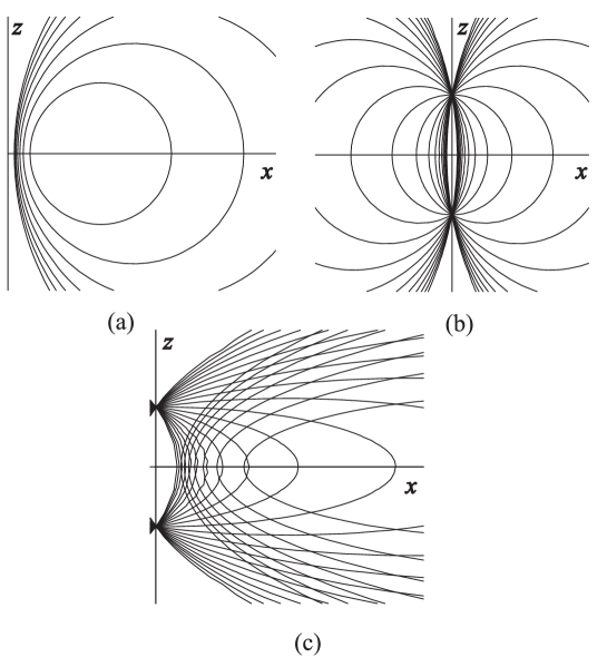
Figure 1. The coordinate net $(s_{1},s_{2})$.

We now establish the connection with the rigid body configuration space (2.12) and find the image of it on the $(s_{1},s_{2})$-plane. To this end, choose the parameters $p,r$ according to (2.17). Introduce the variables $x,y,z$ as follows

$$x^{2}=x_{1}x_{2},\quad y^{2}=y_{1}y_{2},\quad z^{2}=z_{1}z_{2}.$$ (2.29)

Then due to (2.19) we obtain the ellipsoid

$$x^{2}+y^{2}+2z^{2}=2p^{2}.$$

From (2.19) express

$$y_{1}y_{2}=2p^{2}-x^{2}-2z^{2}$$ (2.30)

and represent (2.18) in the form

$$\begin{array}[]{l}(z_{1}+z_{2})^{2}=2r^{2}-(x_{1}y_{2}+x_{2}y_{1})+2z^{2},\\ (z_{1}-z_{2})^{2}=2r^{2}-(x_{1}y_{2}+x_{2}y_{1})-2z^{2}.\end{array}$$ (2.31)

Elimination of the variables $z_{1},z_{2}$ and the product $y_{1}y_{2}$ in (2.18), (2.19), (2.30) gives

$$r^{2}(x_{1}y_{2}+x_{2}y_{1})=r^{4}+2p^{2}x^{2}-(x^{2}+z^{2})^{2}.$$ (2.32)

Denote

$$\Phi_{\pm}(x,z)=(x^{2}+z^{2}\pm r^{2})^{2}-2(p^{2}\pm r^{2})x^{2}.$$

Then (2.31), (2.32) yield the following expressions:

$$r^{2}(z_{1}+z_{2})^{2}=\Phi_{+}(x,z),\quad r^{2}(z_{1}-z_{2})^{2}=\Phi_{-}(x,z).$$ (2.33)

Therefore, the region for $x,z$ is defined by the inequalities

$$\Phi_{+}(x,z)\geqslant 0,\quad\Phi_{-}(x,z)\leqslant 0.$$ (2.34)

Define $s_{1},s_{2}$ as in (2.27) with the chosen $r$. Then

$$s_{1}=\displaystyle{\frac{x^{2}+z^{2}+r^{2}}{2x}},\quad s_{2}=\displaystyle{\frac{x^{2}+z^{2}-r^{2}}{2x}}.$$ (2.35)

The conditions (2.34) take the form

$$s_{1}^{2}\geqslant a^{2},\quad s_{2}^{2}\leqslant b^{2}.$$ (2.36)

This rectangular area (in the above mentioned generalized sense) is the image of the phase space $\mathcal{P}$ under the projection $({\boldsymbol{\omega}},{\boldsymbol{\alpha}},{\boldsymbol{\beta}})\mapsto({\boldsymbol{\alpha}},{\boldsymbol{\beta}})\mapsto(s_{1},s_{2})$. The image of $\mathcal{P}$ on the $(x,z)$-plane with the corresponding part of the $(s_{1},s_{2})$-net is shown in Fig. 2 for the first quadrant.

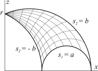
Figure 2. The image of the phase space.

2.3.2. The coordinates $t_{1},t_{2}$

Consider the plane with coordinates $(\xi,x)$ and the second order curve

$$\frac{{\xi^{2}}}{\sigma}+\frac{{x^{2}}}{\tau}=1,$$ (2.37)

where $\tau,\sigma$ are not simultaneously negative. Let $(\xi,x)$ be an arbitrary point of the region

$$\tau\xi^{2}+\sigma x^{2}>\tau\sigma.$$ (2.38)

Then from this point we can draw exactly two tangent lines to the curve (2.37). In other words, the system of tangent lines to the curve (2.37) provides, in the region (2.38), the net of straight lines such that each point belongs to exactly two lines of this net (see Fig. 3). This fact is well-known in geometry.

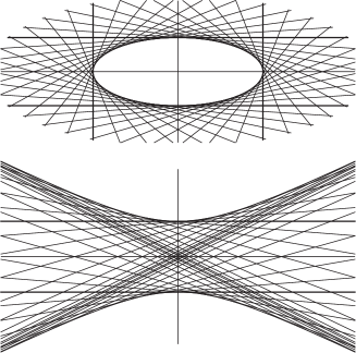
Figure 3. The net of tangent lines to a second order curve.

To describe this net, introduce the variables $t_{1},t_{2}$ as the roots of the quadratic equation

$$t^{2}-\frac{{2\tau\xi}}{{\tau-x^{2}}}t+\frac{{\tau\xi^{2}+\sigma x^{2}}}{{\tau-x^{2}}}=0.$$ (2.39)

Its discriminant is positive in the region (2.38), hence the following expressions are real,

$$t_{1}=\frac{{\tau\xi+\mu x}}{{\tau-x^{2}}},\quad t_{2}=\frac{{\tau\xi-\mu x}}{{\tau-x^{2}}}.$$ (2.40)

Here $\mu=\sqrt{\tau\xi^{2}+\sigma x^{2}-\tau\sigma}\in{\mathbf{R}}$.

Let us also introduce the connection between two coordinate systems $(t_{1},t_{2})$ and $(s_{1},s_{2})$. It will be useful below. Let $p,r,a,b$ satisfy (2.17). In (2.37) we put

$$\sigma=\tau^{2}-2p^{2}\tau+r^{4}$$

and let the coordinates $\xi,x$ depend on $(s_{1},s_{2})$

$$\xi=\frac{{s_{1}+s_{2}}}{{s_{1}-s_{2}}}r^{2}-\tau,\quad x=\frac{{r^{2}}}{{s_{1}-s_{2}}}.$$ (2.41)

With respect to the variables (2.29) we get

$$\xi=x^{2}+z^{2}-\tau.$$ (2.42)

Then the boundary lines of the region (2.36)

$$s_{1}=\pm a,\quad s_{2}=\pm b$$ (2.43)

appear to be coordinate lines in the net $(t_{1},t_{2})$:

$$t_{1}=-\tau\pm r^{2},\quad t_{2}=-\tau\mp r^{2}.$$

3. Example of a geometry based elliptic separation

Here we present the result announced in [25, 26]. Complete investigation including the study of the phase topology can be found in [27].

Consider the second critical subsystem and fix the constants of the first integrals (2.22):

$$M=m,\quad L=\ell.$$ (3.1)

Eliminate from (2.21), (2.18), (2.19) and (3.1) the variables $w_{1},w_{2},w_{3},y_{1},y_{2}$ and the sum ${z_{1}+z_{2}}$. The result is one equation containing $x_{1},x_{2}$ and the product ${z_{1}z_{2}}$:

$${\frac{1}{x_{1}x_{2}}}\Bigl{[}m(x_{1}x_{2}+z_{1}z_{2})+\sqrt{r^{4}m^{2}-r^{2}m(x_{1}+x_{2})+x_{1}x_{2}}\Bigr{]}^{2}=\ell^{2}.$$ (3.2)

It defines a two-dimensional surface in $\mathbf{R}^{3}(\operatorname{\mathfrak{Im}}x_{1},\operatorname{\mathfrak{Re}}x_{1},z)$. Introducing the polar angle $\phi$ by putting $x_{1}+x_{2}=2x\cos\phi$ we obtain the equation on the cylinder $\mathbf{R}^{2}(x,z){\times}S^{1}(\phi\mathop{\rm mod}\nolimits 2\pi)$:

$$m(x^{2}+z^{2})+\sqrt{r^{4}m^{2}-2r^{2}mx\cos\phi+x^{2}}\pm\ell x=0.$$

According to Proposition 1, the generalized boundary of the projection onto the $(x,z)$-plane of a set given by an equation of the type ${f(x,z,\phi)=0}$ without any restrictions on $\phi$ is defined by the condition $\partial f/\partial\phi=0$. In our case since the main equation contains only $\cos\phi$, this condition immediately gives $\sin\phi=0$. Then on the generalized boundary

$$m(x^{2}+z^{2})+|r^{2}m\pm x|\pm\ell x=0.$$

Hence

$$x^{2}+z^{2}\pm r^{2}\pm\frac{{\ell\pm 1}}{m}x=0.$$

Recalling the definition (2.27) we see that for any combination of signs these curves on the $(x,z)$-plane become the coordinate lines of the $(s_{1},s_{2})$-net. In particular, all integral manifolds (3.1) have rectangular images on the $(s_{1},s_{2})$-plane (possibly unbounded if the value $x=0$ equivalent to $s_{1}=\infty$ is admissible). Let us show that this fact indeed leads to separation of variables.

Write the equations (2.13) for the variables (2.15):

$$\begin{array}[]{ll}{x^{\prime}_{1}=-x_{1}w_{3}+z_{1}w_{1},}&{x^{\prime}_{2}=x_{2}w_{3}-z_{2}w_{2},}\\ {y^{\prime}_{1}=-y_{1}w_{3}+z_{2}w_{1},}&{y^{\prime}_{2}=y_{2}w_{3}-z_{1}w_{2},}\\ {2z^{\prime}_{1}=x_{1}w_{2}-y_{2}w_{1},}&{2z^{\prime}_{2}=-x_{2}w_{1}+y_{1}w_{2},}\\ 2w^{\prime}_{1}=-w_{1}(w_{3}-\lambda)-z_{1},&{}\\ 2w^{\prime}_{2}=w_{2}(w_{3}-\lambda)+z_{2},&{}\\ 2w^{\prime}_{3}=y_{2}-y_{1}.&{}\end{array}$$ (3.3)

Here prime stands for $d/d(\mathrm{i}\,t)$. Calculating the derivatives by virtue of these equations we get

$$\begin{array}[]{l}\displaystyle{\bigl{(}\frac{1}{x}\bigr{)}^{\prime}=\frac{1}{{2(x_{1}x_{2})^{3/2}}}(x_{1}z_{2}w_{2}-x_{2}z_{1}w_{1}),}\\[11.38109pt] \displaystyle{\bigl{(}\frac{{x^{2}+z^{2}}}{x}\bigr{)}^{\prime}=\frac{1}{{2(x_{1}x_{2})^{3/2}}}[x_{1}z_{1}(z_{2}^{2}+y_{2}x_{1})w_{2}-x_{2}z_{2}(z_{1}^{2}+y_{1}x_{2})w_{1}].}\end{array}$$ (3.4)

Taking into account (3.1), we obtain from (2.28)

$$\begin{array}[]{l}\displaystyle{s^{\prime}_{1}=\frac{{r^{2}}}{{4x^{2}}}(z_{1}+z_{2})\bigl{[}\sqrt{\frac{{x_{1}}}{{x_{2}}}}w_{2}-\sqrt{\frac{{x_{2}}}{{x_{1}}}}w_{1}\bigr{]},}\\ \displaystyle{s^{\prime}_{2}=\frac{{r^{2}}}{{4x^{2}}}(z_{1}-z_{2})\bigl{[}\sqrt{\frac{{x_{1}}}{{x_{2}}}}w_{2}+\sqrt{\frac{{x_{2}}}{{x_{1}}}}w_{1}\bigr{]}.}\end{array}$$ (3.5)

Denote

$$R_{1}=\sqrt{r^{2}m-x_{1}},\qquad R_{2}=\sqrt{r^{2}m-x_{2}}$$

and express from (2.21)

$$\sqrt{\frac{{x_{1}}}{{x_{2}}}}w_{2}=R_{1},\quad\sqrt{\frac{{x_{2}}}{{x_{1}}}}w_{1}=R_{2}.$$ (3.6)

Equation (3.2) takes the form

$$m(x^{2}+z^{2})+R_{1}R_{2}=\ell x.$$ (3.7)

It follows from the definition of $R_{1},R_{2}$ that

$$\begin{array}[]{l}R_{1}^{2}+R_{2}^{2}=2r^{2}m-(x_{1}+x_{2}),\\ R_{1}^{2}R_{2}^{2}=r^{4}m^{2}-2r^{2}m(x_{1}+x_{2})+x^{2}.\end{array}$$ (3.8)

Therefore from (3.7) we obtain

$$\begin{array}[]{l}R_{1}R_{2}=\ell x-m(x^{2}+z^{2}),\\ \displaystyle{R_{1}^{2}+R_{2}^{2}=\frac{1}{{r^{2}m}}\bigl{\{}[\ell x-m(x^{2}+z^{2})]^{2}-x^{2}\bigr{\}}+r^{2}m.}\end{array}$$

Using the expressions of $x$, $x^{2}+z^{2}$ via $s_{1},s_{2}$, we find

$$\displaystyle{(R_{1}\pm R_{2})^{2}=\frac{{r^{2}}}{{m(s_{1}-s_{2})^{2}}}\{(\ell^{2}-1)-2\ell m[(s_{1}+s_{2})}$$

$$\qquad\mp(s_{1}-s_{2})]+2m^{2}[(s_{1}^{2}+s_{2}^{2})\mp(s_{1}^{2}-s_{2}^{2})]\}.$$ (3.9)

Introduce the following notation:

$$\begin{array}[]{l}\displaystyle{\Psi(s_{1},s_{2})=4ms_{1}s_{2}-2\ell(s_{1}+s_{2})+\displaystyle{\frac{1}{m}}(\ell^{2}-1),}\\[8.53581pt] \displaystyle{\Phi(s)=\Psi(s,s)=4ms^{2}-4\ell s+\frac{1}{m}(\ell^{2}-1).}\end{array}$$ (3.10)

Then from (3.9),

$$\begin{array}[]{l}\displaystyle{R_{1}+R_{2}=\frac{r}{{s_{1}-s_{2}}}\sqrt{\Phi(s_{2})},}\qquad\displaystyle{R_{1}-R_{2}=\frac{r}{{s_{1}-s_{2}}}\sqrt{\Phi(s_{1})}}\end{array}$$ (3.11)

(the radicals may have arbitrary signs). From (2.33) we get

$$\begin{array}[]{l}\displaystyle{(z_{1}+z_{2})^{2}=\frac{{4r^{2}}}{{(s_{1}-s_{2})^{2}}}(s_{1}^{2}-a^{2}),}\qquad\displaystyle{(z_{1}-z_{2})^{2}=\frac{{4r^{2}}}{{(s_{1}-s_{2})^{2}}}(s_{2}^{2}-b^{2}).}\end{array}$$

Hence

$${z_{1}+z_{2}=\frac{{2r}}{{s_{1}-s_{2}}}\sqrt{s_{1}^{2}-a^{2}},}\qquad\displaystyle{z_{1}-z_{2}=\frac{{2r}}{{s_{1}-s_{2}}}\sqrt{s_{2}^{2}-b^{2}},}$$ (3.12)

where the signs of the radicals, similar to (3.11), are arbitrary.

Substitute (3.6), (3.10), (3.12) in (3.5) and return to the real time derivative to obtain the equations describing the time evolution of the auxiliary variables $s_{1},s_{2}$:

$$\begin{array}[]{l}\displaystyle{\frac{{ds_{1}}}{{dt}}=\frac{1}{2}\sqrt{\vphantom{\bigl{(}}s_{1}^{2}-a^{2}}\sqrt{\vphantom{\bigl{(}}-\Phi(s_{1})},}\qquad\displaystyle{\frac{{ds_{2}}}{{dt}}=\frac{1}{2}\sqrt{\vphantom{\bigl{(}}b^{2}-s_{2}^{2}}\sqrt{\vphantom{\bigl{(}}\Phi(s_{2})}.}\end{array}$$ (3.13)

In these equations the variables are separated and the equations themselves are easily integrated in Jacobi’s elliptic functions.

To accomplish the separation, it is necessary to present the expressions of all phase variables in terms of the separated ones. The values $z_{1},z_{2}$ are found from (3.12). From (2.27)

$$\begin{array}[]{l}x=\displaystyle{\frac{r^{2}}{s_{1}-s_{2}}},\qquad x^{2}+z^{2}=r^{2}\displaystyle{\frac{s_{1}+s_{2}}{s_{1}-s_{2}}},\end{array}$$

then $x_{1},x_{2}$ are found from (3.8) and (3.11). The equations (2.18) serve to define $y_{1},y_{2}$, and $w_{1},w_{2}$ are expressed from (3.6). Finally, the variable $w_{3}$ is defined from the first equation (2.21). Thus, for the complex phase variables we have

$$\begin{array}[]{l}\displaystyle{x_{1}=-\frac{{r^{2}}}{{2(s_{1}-s_{2})^{2}}}[\Psi(s_{1},s_{2})+\sqrt{\Phi(s_{1})\Phi(s_{2})}],}\\[8.53581pt] \displaystyle{x_{2}=-\frac{{r^{2}}}{{2(s_{1}-s_{2})^{2}}}[\Psi(s_{1},s_{2})-\sqrt{\Phi(s_{1})\Phi(s_{2})}],}\\[8.53581pt] \displaystyle{y_{1}=2\frac{{(2s_{1}s_{2}-p^{2})-2\sqrt{(s_{1}^{2}-a^{2})(s_{2}^{2}-b^{2})}}}{{\Psi(s_{1},s_{2})-\sqrt{\Phi(s_{1})\Phi(s_{2})}}},}\\[11.38109pt] \displaystyle{y_{2}=2\frac{{(2s_{1}s_{2}-p^{2})+2\sqrt{(s_{1}^{2}-a^{2})(s_{2}^{2}-b^{2})}}}{{\Psi(s_{1},s_{2})+\sqrt{\Phi(s_{1})\Phi(s_{2})}}},}\\[11.38109pt] \displaystyle{z_{1}=\frac{r}{{s_{1}-s_{2}}}(\sqrt{s_{1}^{2}-a^{2}}+\sqrt{s_{2}^{2}-b^{2}}),}\\[8.53581pt] \displaystyle{z_{2}=\frac{r}{{s_{1}-s_{2}}}(\sqrt{s_{1}^{2}-a^{2}}-\sqrt{s_{2}^{2}-b^{2}})}\end{array}$$

and

$$\begin{array}[]{l}\displaystyle{w_{1}=r\frac{{\sqrt{\Phi(s_{2})}-\sqrt{\Phi(s_{1})}}}{{\Psi(s_{1},s_{2})-\sqrt{\Phi(s_{1})\Phi(s_{2})}}},}\\[11.38109pt] \displaystyle{w_{2}=r\frac{{\sqrt{\Phi(s_{2})}+\sqrt{\Phi(s_{1})}}}{{\Psi(s_{1},s_{2})+\sqrt{\Phi(s_{1})\Phi(s_{2})}}},}\\[11.38109pt] \displaystyle{w_{3}=\frac{1}{{s_{1}-s_{2}}}[\sqrt{(s_{2}^{2}-b^{2})\Phi(s_{1})}-\sqrt{(s_{1}^{2}-a^{2})\Phi(s_{2})}].}\end{array}$$

Denote

$$\begin{array}[]{l}\displaystyle{S_{1}=\sqrt{s_{1}^{2}-a^{2}},}\quad\displaystyle{\varphi_{1}=\sqrt{\vphantom{\bigl{(}}-\Phi(s_{1})},}\quad\displaystyle{S_{2}=\sqrt{b^{2}-s_{2}^{2}},}\quad\displaystyle{\varphi_{2}=\sqrt{\vphantom{\bigl{(}}\Phi(s_{2})}.}\end{array}$$ (3.15)

Then

$$\begin{array}[]{l}\displaystyle{\alpha_{1}=\frac{\mathstrut 1}{{2(s_{1}-s_{2})^{2}}}[(s_{1}s_{2}-a^{2})\Psi+S_{1}S_{2}\varphi_{1}\varphi_{2}],}\\ \displaystyle{\alpha_{2}=\frac{\mathstrut 1}{{2(s_{1}-s_{2})^{2}}}[(s_{1}s_{2}-a^{2})\varphi_{1}\varphi_{2}-S_{1}S_{2}\Psi],}\\ \displaystyle{\beta_{1}=-\frac{\mathstrut 1}{{2(s_{1}-s_{2})^{2}}}[(s_{1}s_{2}-b^{2})\varphi_{1}\varphi_{2}-S_{1}S_{2}\Psi],}\\ \displaystyle{\beta_{2}=\frac{\mathstrut 1}{{2(s_{1}-s_{2})^{2}}}[(s_{1}s_{2}-b^{2})\Psi+S_{1}S_{2}\varphi_{1}\varphi_{2}],}\\ \displaystyle{\alpha_{3}=\frac{\mathstrut r}{{s_{1}-s_{2}}}S_{1},\quad\beta_{3}=\frac{r}{{s_{1}-s_{2}}}S_{2},}\\ \displaystyle{\omega_{1}=\frac{\mathstrut r}{{2(s_{1}-s_{2})}}(\ell-2ms_{1})\varphi_{2},\quad\omega_{2}=\frac{r}{{2(s_{1}-s_{2})}}(\ell-2ms_{2})\varphi_{1},}\\ \displaystyle{\omega_{3}=\frac{\mathstrut 1}{{s_{1}-s_{2}}}(S_{2}\varphi_{1}-S_{1}\varphi_{2})}.\end{array}$$ (3.23)

Together with the differential equations (3.13) this gives the complete analytical solution of the problem.

4. Example of a hyperelliptic separation

4.1. The geometry of accessible regions

Let us consider the dynamical system defined by the equations (2.13) on the invariant almost everywhere four-dimensional manifold $\mathcal{M}_{3}$ cut in $\mathbf{R}^{9}$ by five equations (2.18), (2.19), (2.24). This system is Hamiltonian with two degrees of freedom except for the zero-measure set of points where either the equations (2.24) fail to be independent, or the induced symplectic structure degenerates [28]. The possibility of separation of variables was predicted in [21] basing on the above shown geometrical speculations, but it took a long time to obtain the final analytical expressions, complex first [28] and finally real [29].

The functions $S,T$ defined by (2.25) provide the complete set of integrals in involution on $\mathcal{M}_{3}$. In particular, the equations of the integral manifold

$$\{\zeta\in\mathcal{P}:H(\zeta)=h,K(\zeta)=k,G(\zeta)=g\}$$

with the functions (2.16) are replaced with the invariant relations (2.24) and the system of equations

$$S=s,\;T=\tau.$$ (4.1)

Using the variables (2.15) we transform the system (2.24), (4.1) to the form

$$\begin{array}[]{l}(y_{2}+2s)w_{1}+x_{1}w_{2}+z_{1}w_{3}=0,\\ x_{2}w_{1}+(y_{1}+2s)w_{2}+z_{2}w_{3}=0,\\ x_{2}z_{1}w_{1}+x_{1}z_{2}w_{2}+(\tau-x_{1}x_{2})w_{3}=0,\\ 2sw_{1}w_{2}-(x_{1}x_{2}+z_{1}z_{2})+\tau=0.\end{array}$$ (4.2)

Using the variables (2.15) with the corresponding dynamics (3.3) note that despite the complexity of these variables their space is 9-dimensional since the pairs ${(x_{1},x_{2})}$, ${(y_{1},y_{2})}$ and ${(z_{1},z_{2})}$ are complex conjugate and $w_{3}$ is in fact real. Seven relations (4.2), (2.18) and (2.19) define in this space the integral manifold $\mathcal{F}_{s,\tau}$. If the latter set does not have any points of dependence of the functions $S,T$, then it will consist of two-dimensional tori bearing the quasi-periodic motions.

From what follows, we exclude the four points of equilibria on $\mathcal{P}$. At non-trivial motions we have ${\boldsymbol{\omega}}\neq 0$ for almost all time moments. Then the determinant of the first three equations (4.2) in $w_{i}$ ${(i=1,2,3)}$ is identically zero. Eliminate in this condition the variables $z_{1}^{2},z_{2}^{2}$ and the product $y_{1}y_{2}$ with (2.18), (2.19) and (2.30) to obtain

$$\begin{array}[]{l}2s[(r^{2}x_{1}-\tau y_{1})+(r^{2}x_{2}-\tau y_{2})]=-r^{2}(x_{1}y_{2}+x_{2}y_{1})\\ \qquad\qquad+2[2s^{2}(\tau-x^{2})+p^{2}(\tau+x^{2})-\tau(x^{2}+z^{2})].\end{array}$$ (4.3)

On the other hand, it follows from (2.29), (2.30) that

$$(r^{2}x_{1}-\tau y_{1})(r^{2}x_{2}-\tau y_{2})=r^{4}x^{2}+\tau(2p^{2}-x^{2}-2z^{2})-r^{2}\tau(x_{1}y_{2}+x_{2}y_{1}).$$ (4.4)

Denote

$$\sigma=\tau^{2}-2p^{2}\tau+r^{4},\quad\chi=\sqrt{k}\geqslant 0.$$ (4.5)

We have, from the second equation (2.26),

$$4s^{2}\chi^{2}=\sigma+4s^{2}\tau.$$

Introduce the complex conjugate pair

$$\mu_{1}=r^{2}x_{1}-\tau y_{1},\quad\mu_{2}=r^{2}x_{2}-\tau y_{2}$$ (4.6)

and denote for brevity

$$\xi=x^{2}+z^{2}-\tau.$$ (4.7)

Eliminate in (4.3), (4.4) the term $x_{1}y_{2}+x_{2}y_{1}$ by (2.32):

$$\begin{array}[]{c}2s(\mu_{1}+\mu_{2})=\xi^{2}-4s^{2}(x^{2}-\tau)-\sigma,\quad\mu_{1}\mu_{2}=\tau\xi^{2}+\sigma x^{2}-\tau\sigma.\end{array}$$ (4.8)

These two equations in four variables describe the integral manifold $\mathcal{F}_{s,\tau}$ in the space $(x,\xi,\mu_{1},\mu_{2})$ ($\mu_{2}=\overline{\mu_{1}}$). According to Proposition 1, at the points covering the generalized boundary of the projection of $\mathcal{F}_{s,\tau}$ onto the $(x,\xi)$-plane the Jacobian of the system with respect to the variables $\mu_{1},\mu_{2}$ equals zero, or in view of (4.5),

$$(\xi-2sx-2s\chi)(\xi-2sx+2s\chi)(\xi+2sx-2s\chi)(\xi+2sx+2s\chi)=0.$$

So, the straight lines

$$\xi\pm 2sx\pm 2s\chi=0$$ (4.9)

together with (2.43) bound the projection of the integral manifold onto the $(x,\xi)$-plane. Comparing (4.7) with (2.42) recall that the boundary lines of the region (2.36) after the change (2.35) become tangent to the second order curve

$$\tau\xi^{2}+\sigma x^{2}-\tau\sigma=0.$$ (4.10)

The resultant in $\xi$ of any of the equation (4.9) with (4.10) depending on the chosen signs evaluates to $4s^{2}(\tau\pm\chi x)^{2}$. Hence all straight lines (4.9) are also tangent to the curve (4.10), namely, at the points with $x=\mp\tau/\chi$.

Choose $\lambda_{1}=\sqrt{2s\mu_{1}+\sigma}$, $\lambda_{2}=\sqrt{2s\mu_{2}+\sigma}$ to be complex conjugate. Then the system (4.8) simplifies

$$(\lambda_{1}+\lambda_{2})^{2}=\Xi_{+}(x,z),\quad(\lambda_{1}-\lambda_{2})^{2}=\Xi_{-}(x,z).$$

Here

$$\Xi_{\pm}(x,z)=(x^{2}+z^{2}-\tau\pm 2s\chi)^{2}-4s^{2}x^{2},$$

and the solution exists if and only if

$$\Xi_{+}(x,z)\geqslant 0,\quad\Xi_{-}(x,z)\leqslant 0.$$ (4.11)

The inequalities (2.34), (4.11) describe the corresponding accessible region $\mathop{\rm Acc}\nolimits(s,\tau)$ on the $(x,z)$-plane. We now present this region in the plane of the variables $(s_{1},s_{2})$. Express

$$\begin{array}[]{c}\displaystyle{x^{2}+z^{2}-\tau=[s_{1}+s_{2}-\displaystyle{\frac{\tau}{r^{2}}}(s_{1}-s_{2})]x,}\\ \displaystyle{\Xi_{+}(x,z)=x^{2}\Lambda_{+}\Lambda_{-},\quad\Xi_{-}(x,z)=x^{2}{\rm M}_{+}{\rm M}_{-},}\end{array}$$ (4.12)

where

$$\begin{array}[]{l}\displaystyle{\Lambda_{\pm}(s_{1},s_{2})=s_{1}+s_{2}-\displaystyle{\frac{\tau-2s\chi}{r^{2}}}(s_{1}-s_{2})\pm 2s,}\\[11.38109pt] \displaystyle{{\rm M}_{\pm}(s_{1},s_{2})=s_{1}+s_{2}-\displaystyle{\frac{\tau+2s\chi}{r^{2}}}(s_{1}-s_{2})\pm 2s.}\end{array}$$

From (4.11), (4.12) we have

$$\Lambda_{+}(s_{1},s_{2})\Lambda_{-}(s_{1},s_{2})\geqslant 0,\quad{\rm M}_{+}(s_{1},s_{2}){\rm M}_{-}(s_{1},s_{2})\leqslant 0.$$ (4.13)

The lines $\Lambda_{\pm}=0,\;{\rm M}_{\pm}=0$ form a parallelogram. The solutions of (4.13) fill two half-strips attached to its sides belonging to the lines $\Lambda_{\pm}=0$. Moreover, the solutions of (2.36) fill two horizontal half-strips attached to the sides $s_{2}=\pm b$ of the rectangle with vertices $s_{1}=\pm a$, $s_{2}=\pm b$. The intersection of these sets give the accessible region for the variables $s_{1},s_{2}$ (e.g. see Fig. 4 for $a=1$, $b=0.4$, $\tau=1.2$, $s=-0.6$). With respect to these variables all boundary lines are also tangent to the second order curve, which is the image of the curve (4.10) under the change (2.41).

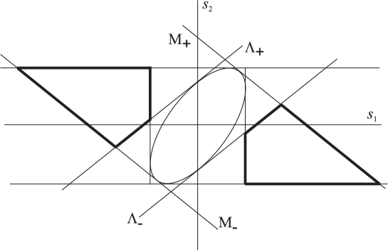
Figure 4. Example of an accessible region.

The presented geometry on the planes $(x,z)$, $(x,\xi)$ and $(s_{1},s_{2})$ shows that it is possible to separate the variables by use of the second coordinate system (2.40), where the notation have the sense given in this section.

4.2. Parametric equations of integral manifolds

At the two-dimensional surface (4.1) the phase variables (2.15) can be expressed in terms of two. At this moment it is convenient to choose for that the variables $x,\xi$. Then from the equations (4.8) we have

$$\begin{array}[]{l}\displaystyle{(\mu_{1}-2s\tau)+(\mu_{2}-2s\tau)=\frac{\xi^{2}}{2s}-2s(x^{2}+\chi^{2})},\\[7.11317pt] \displaystyle{(\mu_{1}-2s\tau)(\mu_{2}-2s\tau)=4s^{2}\chi^{2}x^{2}}.\end{array}$$

Hence

$${\mu_{1}=2s\tau+\frac{1}{8s}(\sqrt{\Psi_{1}}+\sqrt{\Psi_{2}})^{2},\quad\mu_{2}=2s\tau+\frac{1}{8s}(\sqrt{\Psi_{1}}-\sqrt{\Psi_{2}})^{2}.}$$ (4.14)

Here we denote

$$\Psi_{1}(x,\xi)=\xi^{2}-4s^{2}(x+\chi)^{2},\quad\Psi_{2}(x,\xi)=\xi^{2}-4s^{2}(x-\chi)^{2}.$$

From (2.30) we have

$$y_{1}y_{2}=2p^{2}-2(\xi+\tau)+x^{2}.$$

Consider this equation together with the definition $x_{1}x_{2}=x^{2}$ and the equations (4.6). In view of (4.14) we get

$$\begin{array}[]{l}\displaystyle{x_{1}=\frac{2s}{r^{2}}\frac{4r^{4}(x^{2}-\tau)+\tau(\sqrt{\mathstrut\Phi_{1}}+\sqrt{\mathstrut\Phi_{2}})^{2}}{16s^{2}\tau+(\sqrt{\mathstrut\Psi_{1}}-\sqrt{\mathstrut\Psi_{2}})^{2}},}\\[11.38109pt] \displaystyle{x_{2}=\frac{2s}{r^{2}}\frac{4r^{4}(x^{2}-\tau)+\tau(\sqrt{\mathstrut\Phi_{1}}-\sqrt{\mathstrut\Phi_{2}})^{2}}{16s^{2}\tau+(\sqrt{\mathstrut\Psi_{1}}+\sqrt{\mathstrut\Psi_{2}})^{2}},}\end{array}$$ (4.17)

$$\begin{array}[]{l}\displaystyle{y_{1}=2s\frac{4[2\tau\xi-\tau(x^{2}-\tau)+\sigma]-(\sqrt{\mathstrut\Phi_{1}}-\sqrt{\mathstrut\Phi_{2}})^{2}}{16s^{2}\tau+(\sqrt{\mathstrut\Psi_{1}}-\sqrt{\mathstrut\Psi_{2}})^{2}},}\\[11.38109pt] \displaystyle{y_{2}=2s\frac{4[2\tau\xi-\tau(x^{2}-\tau)+\sigma]-(\sqrt{\mathstrut\Phi_{1}}+\sqrt{\mathstrut\Phi_{2}})^{2}}{16s^{2}\tau+(\sqrt{\mathstrut\Psi_{1}}+\sqrt{\mathstrut\Psi_{2}})^{2}}.}\end{array}$$ (4.20)

Here the polynomials

$$\begin{array}[]{c}\Phi_{1}(x,\xi)=(\xi+\tau+r^{2})^{2}-2(p^{2}+r^{2})x^{2},\\ \Phi_{2}(x,\xi)=(\xi+\tau-r^{2})^{2}-2(p^{2}-r^{2})x^{2}\end{array}$$ (4.21)

are obtained from $\Phi_{\pm}$ after substituting $z^{2}$ with its value from (4.7). In the sequel such substitution is supposed by default. From (2.31) we then get

$${z_{1}=\frac{1}{2r}(\sqrt{\mathstrut\Phi_{1}}+\sqrt{\mathstrut\Phi_{2}}),\quad z_{2}=\frac{1}{2r}(\sqrt{\mathstrut\Phi_{1}}-\sqrt{\mathstrut\Phi_{2}}).}$$ (4.22)

As a result we have the expressions for all phase variables from the so-called configuration group, i.e., determining the orientation of the body. The radicals in (4.17), (4.20), (4.22) have arbitrary signs.

To find the variables $w_{i}$, which are in charge of the angular velocity components, we use the expressions (2.16) for the general integrals $K,H$ and the relations (2.26), which define the constants $k,h$ in terms of $s,\tau$. In view of (4.5) we have

$$K=(w_{1}^{2}+x_{1})(w_{2}^{2}+x_{2})=\chi^{2},$$ (4.23)

$$H=\displaystyle{\frac{1}{2}w_{3}^{2}+w_{1}w_{2}-\frac{1}{2}(y_{1}+y_{2})=s+\frac{p^{2}-\tau}{2s}}.$$ (4.24)

From (4.23), (2.25) we obtain the system

$$\begin{array}[]{l}\displaystyle{x_{2}w_{1}^{2}+x_{1}w_{2}^{2}=-\frac{1}{4s^{2}}[\xi^{2}+4s^{2}(\chi^{2}+x^{2})],}\qquad\displaystyle{w_{1}w_{2}=\frac{\xi}{2s}}.\end{array}$$

Hence

$${w_{1}=\frac{i}{4s\sqrt{x_{2}}}(\sqrt{\mathstrut\Theta_{1}}+\sqrt{\mathstrut\Theta_{2}}),\quad w_{2}=\frac{i}{4s\sqrt{x_{1}}}(\sqrt{\mathstrut\Theta_{1}}-\sqrt{\mathstrut\Theta_{2}}),}$$ (4.25)

where

$$\Theta_{1}(x,\xi)=(\xi-2sx)^{2}-4s^{2}\chi^{2},\quad\Theta_{2}(x,\xi)=(\xi+2sx)^{2}-4s^{2}\chi^{2}.$$ (4.26)

Substitute (4.25), (4.20) into (4.24) to get

$${w_{3}^{2}=\frac{1}{4s\mu^{2}}\bigl{(}P-\sqrt{\Phi_{1}\Phi_{2}\Psi_{1}\Psi_{2}}\bigr{)},}$$ (4.27)

where

$$\begin{array}[]{l}P=4s^{2}(x^{2}-\chi^{2})[2(\tau-p^{2})x^{2}-\tau^{2}+r^{4}]+8s^{2}[(\tau-2\chi^{2})x^{2}+\tau\chi^{2}]\xi\\ \phantom{P=}-2[(\tau-p^{2}-2s^{2})x^{2}+\tau(p^{2}-2s^{2})-r^{4}]\xi^{2}-2\tau\xi^{3}-\xi^{4}.\end{array}$$

Denote

$$Q=(\xi+\tau+2s^{2}-p^{2})^{2}-4s^{2}x^{2}-(p^{2}-2s^{2})^{2}+r^{4}.$$

The following identity holds

$$P^{2}-\Phi_{1}\Phi_{2}\Psi_{1}\Psi_{2}=4x^{2}(\tau\xi^{2}+\sigma x^{2}-\tau\sigma)Q^{2}.$$

Using the second equation (4.8) we find from (4.27)

$${w_{3}=\frac{1}{2\sqrt{2s}\mu}(\sqrt{P_{1}}-\sqrt{P_{2}}),}$$ (4.28)

where

$$P_{1}=P+2x\mu Q,\quad P_{2}=P-2x\mu\delta,\qquad\mu^{2}=\mu_{1}\mu_{2}.$$ (4.29)

Simultaneously, from (4.8),

$$\mu^{2}=\tau\xi^{2}+\sigma x^{2}-\tau\sigma.$$ (4.30)

Thus, the equations (4.17), (4.20), (4.22), (4.25) and (4.28) give the dependencies of all phase variables (2.15) on the two variables $x,\xi$ taken as the intermediate ones.

4.3. The change of variables

Introduce the local coordinates $t_{1},t_{2}$ according to (2.40) on the $(x,\xi)$-plane. The discriminant of the corresponding equation (2.39) now coincides with the value $\mu^{2}$ in (4.29) and is, therefore, non-negative. So the variables $t_{1},t_{2}$ are real. Solve (4.30), (2.40) with respect to $x,\xi,\mu$,

$$\begin{array}[]{c}\displaystyle{x=\frac{\sqrt{\tau}(U_{1}+U_{2})}{t_{1}+t_{2}},}\quad\displaystyle{\xi=\frac{t_{1}t_{2}+\sigma-U_{1}U_{2}}{t_{1}+t_{2}},}\quad\displaystyle{\mu=\frac{\sqrt{\tau}(t_{2}U_{1}-t_{1}U_{2})}{t_{1}+t_{2}}.}\end{array}$$ (4.31)

Here we denote for brevity

$$U_{1}=\sqrt{t_{1}^{2}-\sigma},\quad U_{2}=\sqrt{t_{2}^{2}-\sigma}.$$ (4.32)

Note that the signs of these radicals should be chosen arbitrary to supply, at given $t_{1},t_{2}$, all possible triples $x,\xi,\mu$ in (4.31) satisfying the system (4.30), (2.40). The following easily checked identities simplify some calculation below:

$$\displaystyle{x\mu=\frac{t_{1}-t_{2}}{t_{1}+t_{2}}\,\tau\xi,}$$ (4.33)

$$\displaystyle{\frac{(t_{1}t_{2}+\sigma+U_{1}U_{2})(t_{1}t_{2}+\sigma-U_{1}U_{2})}{(t_{1}+t_{2})^{2}}=\sigma,}$$ (4.34)

$$\displaystyle{\frac{t_{1}t_{2}+\sigma-U_{1}U_{2}}{t_{1}t_{2}-\sigma-U_{1}U_{2}}=\frac{(U_{1}+U_{2})^{2}}{(t_{1}-t_{2})^{2}}.}$$ (4.35)

We begin with $\mu_{1},\mu_{2}$ defining the denominators in (4.17), (4.20). Put $\psi=16s^{2}\tau+\Psi_{1}+\Psi_{2}$. According to (4.14) we have

$$\begin{array}[]{c}\displaystyle{\mu_{1}=\frac{1}{8s}(\psi-2\sqrt{\Psi_{1}\Psi_{2}}),\qquad\mu_{2}=\frac{1}{8s}(\psi+2\sqrt{\Psi_{1}\Psi_{2}})}.\end{array}$$

By definition $\psi^{2}-4\Psi_{1}\Psi_{2}=64s^{2}\mu^{2}$, and we write

$$2\sqrt{\vphantom{\bigl{(}}\Psi_{1}\Psi_{2}}=\sqrt{\vphantom{\bigl{(}}\psi+8s\mu}\sqrt{\vphantom{\bigl{(}}\psi-8s\mu}.$$

Hence

$$\begin{array}[]{l}\displaystyle{\mu_{1}=\frac{1}{16s}(\sqrt{\psi+8s\mu}-\sqrt{\psi-8s\mu})^{2},}\\[8.53581pt] \displaystyle{\mu_{2}=\frac{1}{16s}(\sqrt{\psi+8s\mu}+\sqrt{\psi-8s\mu})^{2}.}\end{array}$$

Substituting (4.31) we get

$$\begin{array}[]{l}\displaystyle{\psi+8s\mu=\frac{4R^{2}\varphi_{1}^{2}\varphi_{2}^{2}}{(t_{1}+t_{2})^{2}},}\qquad\displaystyle{\psi-8s\mu=\frac{4R^{2}\psi_{1}^{2}\psi_{2}^{2}}{(t_{1}+t_{2})^{2}},}\end{array}$$

where

$$\begin{array}[]{l}\varphi_{1}=\sqrt{2s\sqrt{\tau}+U_{1}},\quad\varphi_{2}=\sqrt{2s\sqrt{\tau}+U_{2}},\\ \psi_{1}=\sqrt{2s\sqrt{\tau}-U_{1}},\quad\psi_{2}=\sqrt{2s\sqrt{\tau}-U_{2}}.\end{array}$$

This notation is intermediate, the signs chosen here do not affect the final expressions. The only important value is the new radical

$$R=\sqrt{\vphantom{4s^{2}}t_{1}t_{2}+\sigma+U_{1}U_{2}}.$$ (4.36)

Now the expressions for $\mu_{1},\mu_{2}$ become

$$\begin{array}[]{l}\displaystyle{\mu_{1}=\frac{R^{2}(\varphi_{1}\varphi_{2}-\psi_{1}\psi_{2})^{2}}{4s(t_{1}+t_{2})^{2}},}\qquad\displaystyle{\mu_{2}=\frac{R^{2}(\varphi_{1}\varphi_{2}+\psi_{1}\psi_{2})^{2}}{4s(t_{1}+t_{2})^{2}}.}\end{array}$$ (4.37)

We can avoid “double roots” by using the expanded form:

$$\begin{array}[]{l}\displaystyle{\mu_{1}=\frac{R^{2}(4s^{2}\tau+U_{1}U_{2}-V_{1}V_{2})}{2s(t_{1}+t_{2})^{2}},}\qquad\displaystyle{\mu_{2}=\frac{R^{2}(4s^{2}\tau+U_{1}U_{2}+V_{1}V_{2})}{2s(t_{1}+t_{2})^{2}}.}\end{array}$$ (4.38)

Here we introduce new algebraic radicals

$$V_{1}=\sqrt{\mathstrut 4s^{2}\chi^{2}-t_{1}^{2}},\quad V_{2}=\sqrt{\mathstrut 4s^{2}\chi^{2}-t_{2}^{2}}$$ (4.39)

having arbitrary signs.

To find $x_{1},x_{2}$, in addition to (4.32), (4.36), (4.39) denote

$$\begin{array}[]{ll}M_{1}=\sqrt{\vphantom{r^{2}}t_{1}+\tau+r^{2}},&M_{2}=\sqrt{\vphantom{\bigl{(}}t_{2}+\tau+r^{2}},\\[4.2679pt] N_{1}=\sqrt{\vphantom{r^{2}}t_{1}+\tau-r^{2}},&N_{2}=\sqrt{\vphantom{\bigl{(}}t_{2}+\tau-r^{2}}.\end{array}$$ (4.40)

The signs here are also arbitrary. For the polynomials (4.21) we have

$$\begin{array}[]{l}\displaystyle{\Phi_{1}=\frac{2R^{2}M_{1}^{2}M_{2}^{2}}{(t_{1}+t_{2})^{2}},}\qquad\displaystyle{\Phi_{2}=\frac{2R^{2}N_{1}^{2}N_{2}^{2}}{(t_{1}+t_{2})^{2}}.}\end{array}$$ (4.41)

Let $X=4r^{4}(x^{2}-\tau)+\tau(\Phi_{1}+\Phi_{2})$. Then from (4.41) and (4.34) we find

$$X^{2}-4\tau^{2}\Phi_{1}\Phi_{2}=\frac{16\tau^{2}r^{4}(t_{1}-t_{2})^{2}R^{4}}{(t_{1}+t_{2})^{4}}.$$

Hence $2\tau\sqrt{\mathstrut\Phi_{1}\Phi_{2}}=\sqrt{\mathstrut X_{1}X_{2}}$, where

$$\begin{array}[]{l}\displaystyle{X_{1}=X+\sqrt{X^{2}-4\tau^{2}\Phi_{1}\Phi_{2}}=\frac{4\tau R^{2}N_{1}^{2}M_{2}^{2}}{(t_{1}+t_{2})^{2}},}\\ \displaystyle{X_{2}=X-\sqrt{X^{2}-4\tau^{2}\Phi_{1}\Phi_{2}}=\frac{4\tau R^{2}M_{2}^{2}N_{1}^{2}}{(t_{1}+t_{2})^{2}}.}\end{array}$$

For the numerators in (4.17) we obtain

$$4r^{4}(x^{2}-\tau)+\tau(\sqrt{\Phi_{1}}\pm\sqrt{\Phi_{2}})^{2}=\frac{1}{2}(\sqrt{X_{1}}\pm\sqrt{X_{2}})^{2}.$$

Then from (4.14), (4.17), (4.37) we get

$$\begin{array}[]{l}\displaystyle{x_{1}=\frac{2s\tau}{r^{2}}\left(\frac{M_{2}N_{1}+M_{1}N_{2}}{\varphi_{1}\varphi_{2}+\psi_{1}\psi_{2}}\right)^{2},}\qquad\displaystyle{x_{2}=\frac{2s\tau}{r^{2}}\left(\frac{M_{2}N_{1}-M_{1}N_{2}}{\varphi_{1}\varphi_{2}-\psi_{1}\psi_{2}}\right)^{2},}\end{array}$$ (4.42)

or in the expanded form

$$\begin{array}[]{l}\displaystyle{x_{1}=\frac{2s\tau}{r^{2}}\frac{(t_{1}+\tau)(t_{2}+\tau)-r^{4}+M_{1}N_{1}M_{2}N_{2}}{4s^{2}\tau+U_{1}U_{2}+V_{1}V_{2}},}\\[8.53581pt] \displaystyle{x_{2}=\frac{2s\tau}{r^{2}}\frac{(t_{1}+\tau)(t_{2}+\tau)-r^{4}-M_{1}N_{1}M_{2}N_{2}}{4s^{2}\tau+U_{1}U_{2}-V_{1}V_{2}}.}\end{array}$$ (4.43)

The expressions for $y_{1},y_{2}$ in terms of $t_{1},t_{2}$ are now easily found from the definition (4.6) of $\mu_{1},\mu_{2}$. Write

$$\tau y_{1}\mu_{2}=r^{2}x_{1}\mu_{2}-\mu^{2},\quad\tau y_{2}\mu_{1}=r^{2}x_{2}\mu_{1}-\mu^{2}.$$

Then after substitution of (4.38), (4.43), (4.31) we get

$$\begin{array}[]{l}\displaystyle{y_{1}=2s\frac{\tau(t_{1}+t_{2}-2p^{2}+2\tau)-U_{1}U_{2}+M_{1}N_{1}M_{2}N_{2}}{4s^{2}\tau+U_{1}U_{2}+V_{1}V_{2}},}\\[8.53581pt] \displaystyle{y_{2}=2s\frac{\tau(t_{1}+t_{2}-2p^{2}+2\tau)-U_{1}U_{2}-M_{1}N_{1}M_{2}N_{2}}{4s^{2}\tau+U_{1}U_{2}-V_{1}V_{2}}.}\end{array}$$ (4.44)

The variables $z_{1},z_{2}$ are expressed from (4.21), (4.22):

$$\begin{array}[]{l}\displaystyle{z_{1}=\frac{R}{\sqrt{2}\,r}\frac{M_{1}M_{2}+N_{1}N_{2}}{t_{1}+t_{2}},}\qquad\displaystyle{z_{2}=\frac{R}{\sqrt{2}\,r}\frac{M_{1}M_{2}-N_{1}N_{2}}{t_{1}+t_{2}}.}\end{array}$$ (4.45)

To find the components of the angular velocity, start with $w_{3}$. Using the identity (4.34) represent the polynomials $P,Q$ as follows

$${P=\frac{4\xi^{2}}{(t_{1}+t_{2})^{2}}\,\widetilde{P},\quad Q=\frac{2\xi}{t_{1}+t_{2}}\,\widetilde{Q}.}$$

Here

$$\begin{array}[]{l}\widetilde{P}=-(t_{1}^{2}-r^{4})(t_{2}^{2}-r^{4})+\tau[(2s^{2}-t_{2})t_{1}^{2}+(2s^{2}-t_{1})t_{2}^{2}-p^{2}(t_{1}^{2}+t_{2}^{2})\\ \qquad\qquad+r^{4}(t_{1}+t_{2}-4s^{2}+2p^{2})]+2\tau^{2}(2s^{2}-p^{2})(t_{1}+t_{2})\\ \qquad\qquad+\tau^{3}(t_{1}+t_{2}+4s^{2}-2p^{2})+\tau^{4},\\ \widetilde{Q}=t_{1}t_{2}+(2s^{2}-p^{2})(t_{1}+t_{2})+r^{4}+\tau(t_{1}+t_{2}+4s^{2}-2p^{2})+\tau^{2}.\end{array}$$

In virtue of (4.39), (4.40) we obtain for the functions (4.29)

$$\begin{array}[]{l}\displaystyle{P_{1}=\frac{4\xi^{2}}{(t_{1}+t_{2})^{2}}M_{1}^{2}N_{1}^{2}V_{2}^{2},}\qquad\displaystyle{P_{2}=\frac{4\xi^{2}}{(t_{1}+t_{2})^{2}}M_{2}^{2}N_{2}^{2}V_{1}^{2}.}\end{array}$$

Then from (4.28) using the identity (4.33) we find

$${w_{3}=\frac{U_{1}-U_{2}}{\sqrt{2s\tau}}\frac{M_{2}N_{2}V_{1}-M_{1}N_{1}V_{2}}{t_{1}^{2}-t_{2}^{2}}=\frac{1}{\sqrt{2s\tau}}\frac{M_{2}N_{2}V_{1}-M_{1}N_{1}V_{2}}{U_{1}+U_{2}}}.$$ (4.46)

Note that the expressions for $x_{i},y_{i},z_{i}$ contain only the product $V_{1}V_{2}$. Therefore we can write the signs of the terms in the numerator of $w_{3}$ in different ways. Then, having fixed the form (4.46) and applying (4.25) to find $w_{1},w_{2}$, we must point out the rule to define the signs of the radicals $\sqrt{\Theta_{1}},\sqrt{\Theta_{2}}$ in a way that guarantees all combinations satisfying the system of three equations (4.2) linear in $w_{i}$, together with (4.46). Since the determinant of this system is zero by virtue of (4.3), we need to check only two of these equations, e.g.,

$$\begin{array}[]{l}(y_{2}+2s)w_{1}+x_{1}w_{2}+z_{1}w_{3}=0,\\ x_{2}w_{1}+(y_{1}+2s)w_{2}+z_{2}w_{3}=0.\end{array}$$ (4.47)

From (4.42) we write

$$\begin{array}[]{l}\displaystyle{\sqrt{x_{1}}=\frac{\sqrt{2s\tau}}{r}\frac{M_{2}N_{1}+M_{1}N_{2}}{\varphi_{1}\varphi_{2}+\psi_{1}\psi_{2}},}\qquad\displaystyle{\sqrt{x_{2}}=\frac{\sqrt{2s\tau}}{r}\frac{M_{2}N_{1}-M_{1}N_{2}}{\varphi_{1}\varphi_{2}-\psi_{1}\psi_{2}}.}\end{array}$$

Here the signs are chosen to satisfy the necessary condition $\sqrt{x_{1}}\sqrt{x_{2}}\equiv x$, where the value $x$ is defined according to (4.31). For $\Theta_{1},\Theta_{2}$ the equations (4.26) and (4.31) then give

$$\begin{array}[]{c}(t_{1}+t_{2})^{2}\Theta_{1}=-2R^{2}\varphi_{1}^{2}\psi_{2}^{2},\qquad(t_{1}+t_{2})^{2}\Theta_{2}=-2R^{2}\psi_{1}^{2}\varphi_{2}^{2}.\end{array}$$

Hence, introducing $\varepsilon_{1,2}=\pm 1$ we write

$$\begin{array}[]{c}(t_{1}+t_{2})\sqrt{\mathstrut\Theta_{1}}=\mathrm{i}\,\varepsilon_{1}\,\sqrt{2}R\varphi_{1}\psi_{2},\qquad(t_{1}+t_{2})\sqrt{\mathstrut\Theta_{2}}=\mathrm{i}\,\varepsilon_{2}\,\sqrt{2}R\psi_{1}\varphi_{2}.\end{array}$$

Then

$$\begin{array}[]{l}w_{1}=\displaystyle{\frac{rR}{4s\sqrt{s\tau}}\frac{(\varepsilon_{2}\varphi_{2}^{2}-\varepsilon_{1}\psi_{2}^{2})V_{1}+(\varepsilon_{1}\varphi_{1}^{2}-\varepsilon_{2}\psi_{1}^{2})V_{2}}{(t_{1}+t_{2})(M_{1}N_{2}-M_{2}N_{1})}},\\[8.53581pt] w_{2}=\displaystyle{\frac{rR}{4s\sqrt{s\tau}}\frac{(\varepsilon_{2}\varphi_{2}^{2}-\varepsilon_{1}\psi_{2}^{2})V_{1}-(\varepsilon_{1}\varphi_{1}^{2}-\varepsilon_{2}\psi_{1}^{2})V_{2}}{(t_{1}+t_{2})(M_{1}N_{2}+M_{2}N_{1})}}.\end{array}$$

Choose $\varepsilon_{2}=-\varepsilon_{1}$. The expressions

$$w_{1}=\pm\frac{rR}{\sqrt{s}(t_{1}+t_{2})}\frac{V_{1}-V_{2}}{M_{2}N_{1}-M_{1}N_{2}},\qquad w_{2}=\mp\frac{rR}{\sqrt{s}(t_{1}+t_{2})}\frac{V_{1}+V_{2}}{M_{2}N_{1}+M_{1}N_{2}},$$

do not satisfy (4.47) for any choice of the signs. For $\varepsilon_{1}=\varepsilon_{2}=\varepsilon$ out of two possibilities $\varepsilon=\pm 1$ only one satisfies (4.46) and (4.47), namely,

$$\begin{array}[]{l}\displaystyle{w_{1}=\frac{r(U_{1}V_{2}+U_{2}V_{1})R}{2s\sqrt{s\tau}(t_{1}+t_{2})(M_{2}N_{1}-M_{1}N_{2})}},\\ \displaystyle{w_{2}=\frac{r(U_{1}V_{2}-U_{2}V_{1})R}{2s\sqrt{s\tau}(t_{1}+t_{2})(M_{2}N_{1}+M_{1}N_{2})}}.\end{array}$$ (4.48)

To accomplish the algebraic solution note that we still have a “double root” expression for $R$. In fact, it can be eliminated. Put

$$\varkappa=\sqrt{\sigma}.$$

This value can be either real or pure imaginary. Denote

$$\begin{array}[]{l}K_{1}=\sqrt{\vphantom{\bigl{(}}t_{1}+\varkappa},\quad K_{2}=\sqrt{\vphantom{\bigl{(}}t_{2}+\varkappa},\quad L_{1}=\sqrt{\vphantom{\bigl{(}}t_{1}-\varkappa},\quad L_{2}=\sqrt{\vphantom{\bigl{(}}t_{2}-\varkappa}.\end{array}$$

Then

$$\begin{array}[]{l}R=\displaystyle{\frac{1}{\sqrt{\mathstrut 2}}}(K_{1}K_{2}+L_{1}L_{2}),\qquad U_{1}=K_{1}L_{1},\qquad U_{2}=K_{2}L_{2}.\end{array}$$

Finally, the formulae (4.43), (4.44), (4.45), (4.46) and (4.48) algebraically define the values of complex phase coordinates (2.15) for given $t_{1},t_{2}$ up to the choice of signs for the following radicals

$$\sqrt{s\tau},\,K_{1},\,K_{2},\,L_{1},\,L_{2},\,V_{1},\,V_{2},\,M_{1},\,M_{2},\,N_{1},\,N_{2}.$$

Here $V_{i},M_{i},N_{i}$ can be real or pure imaginary, and the pairs $K_{1},K_{2}$ and $L_{1},L_{2}$ can be real or complex conjugate. Accessible regions for $t_{1},t_{2}$ are defined by the condition that the initial phase variables $\alpha_{j},\beta_{j},\omega_{j}$ $(j=1,2,3)$ in (2.15) are real.

4.4. The equations of motion and the real solution

To derive the differential equations, which describe the time evolution of the variables $t_{1},t_{2}$ let us use the variables $s_{1},s_{2}$ as the intermediate ones. From (2.35), (4.7) we get

$${s_{1}=\frac{\xi+\tau+r^{2}}{2x},}\quad\displaystyle{s_{2}=\frac{\xi+\tau-r^{2}}{2x}.}$$ (4.49)

Calculate the derivatives by virtue of (3.3). Then from (3.4) we obtain

$$\begin{array}[]{l}\displaystyle{\frac{ds_{1}}{dt}=i\frac{r^{2}}{4x^{3}}(z_{1}+z_{2})(x_{1}w_{2}-x_{2}w_{1}),}\\[8.53581pt] \displaystyle{\frac{ds_{2}}{dt}=i\frac{r^{2}}{4x^{3}}(z_{1}-z_{2})(x_{1}w_{2}+x_{2}w_{1}).}\end{array}$$ (4.50)

On the other hand,

$$\begin{array}[]{l}\displaystyle{\frac{ds_{1}}{dt}=\frac{\partial s_{1}}{\partial t_{1}}\frac{dt_{1}}{dt}+\frac{\partial s_{1}}{\partial t_{2}}\frac{dt_{2}}{dt},}\quad\displaystyle{\frac{ds_{2}}{dt}=\frac{\partial s_{2}}{\partial t_{1}}\frac{dt_{1}}{dt}+\frac{\partial s_{2}}{\partial t_{2}}\frac{dt_{2}}{dt}.}\end{array}$$ (4.51)

Substitute (4.31) to (4.49) to obtain

$$\begin{array}[]{ll}\displaystyle{\frac{\partial s_{1}}{\partial t_{1}}=-\frac{t_{1}t_{2}-\sigma+U_{1}U_{2}}{2\sqrt{\tau}(t_{1}-t_{2})^{2}}\frac{M_{2}^{2}}{U_{1}},}&\displaystyle{\frac{\partial s_{1}}{\partial t_{2}}=\frac{t_{1}t_{2}-\sigma+U_{1}U_{2}}{2\sqrt{\tau}(t_{1}-t_{2})^{2}}\frac{M_{1}^{2}}{U_{2}},}\\[11.38109pt] \displaystyle{\frac{\partial s_{2}}{\partial t_{1}}=-\frac{t_{1}t_{2}-\sigma+U_{1}U_{2}}{2\sqrt{\tau}(t_{1}-t_{2})^{2}}\frac{N_{2}^{2}}{U_{1}},}&\displaystyle{\frac{\partial s_{2}}{\partial t_{2}}=\frac{t_{1}t_{2}-\sigma+U_{1}U_{2}}{2\sqrt{\tau}(t_{1}-t_{2})^{2}}\frac{N_{1}^{2}}{U_{2}}.}\end{array}$$ (4.52)

From (4.51), (4.52) we have

$$\begin{array}[]{ll}\displaystyle{\frac{dt_{1}}{dt}=\frac{\sqrt{\tau}(t_{1}-t_{2})U_{1}}{r^{2}(t_{1}t_{2}-\sigma+U_{1}U_{2})}(M_{1}^{2}\frac{ds_{2}}{dt}-N_{1}^{2}\frac{ds_{1}}{dt}),}\\[11.38109pt] \displaystyle{\frac{dt_{2}}{dt}=\frac{\sqrt{\tau}(t_{1}-t_{2})U_{2}}{r^{2}(t_{1}t_{2}-\sigma+U_{1}U_{2})}(M_{2}^{2}\frac{ds_{2}}{dt}-N_{2}^{2}\frac{ds_{1}}{dt}).}\end{array}$$ (4.53)

Express the values (4.50) in terms of $t_{1},t_{2}$ using (4.43), (4.45), (4.48):

$$\begin{array}[]{ll}\displaystyle{\frac{ds_{1}}{dt}=\mathrm{i}\frac{(t_{1}t_{2}+\sigma+U_{1}U_{2})M_{1}M_{2}(M_{1}N_{2}V_{2}-M_{2}N_{1}V_{1})}{2\sqrt{2s}\,\tau(U_{1}-U_{2})^{2}(t_{1}-t_{2})},}\\[8.53581pt] \displaystyle{\frac{ds_{2}}{dt}=\mathrm{i}\frac{(t_{1}t_{2}+\sigma+U_{1}U_{2})N_{1}N_{2}(M_{2}N_{1}V_{2}-M_{1}N_{2}V_{1})}{2\sqrt{2s}\,\tau(U_{1}-U_{2})^{2}(t_{1}-t_{2})}.}\end{array}$$

Substitute these expressions to (4.53). Then in view of the relation (4.35) after some obvious transformations we come to the equations of the Kowalevski type

$$\begin{array}[]{ll}\displaystyle{(t_{1}-t_{2})\frac{dt_{1}}{dt}=\sqrt{\frac{1}{2s\tau}(4s^{2}\chi^{2}-t_{1}^{2})(t_{1}^{2}-\sigma)[r^{4}-(t_{1}+\tau)^{2}]}\,,}\\[8.53581pt] \displaystyle{(t_{1}-t_{2})\frac{dt_{2}}{dt}=\sqrt{\frac{1}{2s\tau}(4s^{2}\chi^{2}-t_{2}^{2})(t_{2}^{2}-\sigma)[r^{4}-(t_{2}+\tau)^{2}]}\,.}\end{array}$$

To obtain the expressions for the real phase variables use the inverse linear mapping to the change (2.15). From (4.43), (4.44), (4.45) we find $\alpha_{j},\beta_{j}$ $(j=1,2,3)$ as functions of $t_{1},t_{2}$:

$$\begin{array}[]{l}\displaystyle{\alpha_{1}=\frac{(\mathcal{A}-r^{2}U_{1}U_{2})(4s^{2}\tau+U_{1}U_{2})-(\tau+r^{2})M_{1}N_{1}M_{2}N_{2}V_{1}V_{2}}{4r^{2}s\,\tau(U_{1}+U_{2})^{2}},}\\[8.53581pt] \displaystyle{\alpha_{2}=\mathrm{i}\frac{(\mathcal{A}-r^{2}U_{1}U_{2})V_{1}V_{2}-(4s^{2}\tau+U_{1}U_{2})(\tau+r^{2})M_{1}N_{1}M_{2}N_{2}}{4r^{2}s\,\tau(U_{1}+U_{2})^{2}},}\\[8.53581pt] \displaystyle{\alpha_{3}=\frac{R}{r\sqrt{\mathstrut 2}}\,\frac{M_{1}M_{2}}{t_{1}+t_{2}},}\\ \displaystyle{\beta_{1}=\mathrm{i}\frac{(\mathcal{B}+r^{2}U_{1}U_{2})V_{1}V_{2}-(4s^{2}\tau+U_{1}U_{2})(\tau-r^{2})M_{1}N_{1}M_{2}N_{2}}{4r^{2}s\,\tau(U_{1}+U_{2})^{2}},}\\[8.53581pt] \displaystyle{\beta_{2}=-\frac{(\mathcal{B}+r^{2}U_{1}U_{2})(4s^{2}\tau+U_{1}U_{2})-(\tau-r^{2})M_{1}N_{1}M_{2}N_{2}V_{1}V_{2}}{4r^{2}s\,\tau(U_{1}+U_{2})^{2}},}\\[8.53581pt] \displaystyle{\beta_{3}=-\mathrm{i}\frac{R}{r\sqrt{\mathstrut 2}}\,\frac{N_{1}N_{2}}{t_{1}+t_{2}}.}\end{array}$$ (4.54)

Here for brevity we put

$$\begin{array}[]{l}\mathcal{A}=[(t_{1}+\tau+r^{2})(t_{2}+\tau+r^{2})-2(p^{2}+r^{2})r^{2}]\tau,\\ \mathcal{B}=[(t_{1}+\tau-r^{2})(t_{2}+\tau-r^{2})+2(p^{2}-r^{2})r^{2}]\tau.\end{array}$$

The angular velocities $\omega_{j}$ $(j=1,2,3)$ are found from (2.15), (4.46), (4.48):

$$\begin{array}[]{l}\displaystyle{\omega_{1}=\frac{R}{4rs\,\sqrt{s\,\tau}}\,\frac{M_{2}N_{1}U_{1}V_{2}+M_{1}N_{2}U_{2}V_{1}}{t_{1}^{2}-t_{2}^{2}},}\\[8.53581pt] \displaystyle{\omega_{2}=-\frac{\mathrm{i}\,R}{4rs\,\sqrt{s\,\tau}}\,\frac{M_{2}N_{1}U_{2}V_{1}+M_{1}N_{2}U_{1}V_{2}}{t_{1}^{2}-t_{2}^{2}},}\\[8.53581pt] \displaystyle{\omega_{3}=\frac{U_{1}-U_{2}}{\sqrt{2s\tau}}\frac{M_{2}N_{2}V_{1}-M_{1}N_{1}V_{2}}{t_{1}^{2}-t_{2}^{2}}.}\end{array}$$ (4.55)

These explicit expressions of the phase variables in terms of the $t_{1},t_{2}$ along with the separated differential equations give the complete analytical solution for the third critical subsystem.

5. Conclusion

In this article we presented the results dealing with analytical solutions in the generalized Kowalevski problem. The questions of qualitative and topological analysis of the arising subsystems are connected with the investigation of the multi-valued dependencies (3.23) and (4.54), (4.55). Formally these dependencies are the inverse mappings for the coverings of degree $2^{n}$, where $n$ is the number of radicals with arbitrary signs. Lately, new methods of investigating the phase topology of algebraically solvable systems were proposed in [30] based on calculating the invariants of some $\mathbb{Z}_{2}$-linear mappings. (When this article was already published a theory of the topological analysis based on Boolean vector-functions was presented in [41, 42] with applications to the classical problems and to the systems described above.)

Up to this moment the first critical subsystem (the Bogoyavlensky case) has not received any analytical solution despite the fact that its topology is completely investigated in [15] and various Lax representations are found in [8, 13]. For the case of the Kowalevski gyrostat in two constant fields no analytical solutions are found except for the special periodic motions and their bifurcations studied in [32], though all critical subsystems are analytically described in [23].

The Kowalevski problem in the rigid body dynamics remains as challenging as it was during the last 120 years.

The Russian version of this article was written with the financial support of the RFBR and the Volgograd Region Administration (grant No 10-01-97001).

References

- [1] A. V. Borisov and I. S. Mamaev, Rigid body dynamics (Izhevsk: RCD Publ., 2001). (In Russian)
- [2] A. V. Borisov and I. S. Mamaev, Rigid body dynamics: Hamilton methods, integrability, chaos (Izhevsk: RCD Publ., 2005). (In Russian)
- [3] A. V. Borisov and I. S. Mamaev, Contemporary methods in the theory of integrable systems (Izhevsk: RCD Publ., 2003). (In Russian)
- [4] A. G. Reyman and M. A. Semenov-Tian-Shansky, Integrable systems. Group theory approach (Izhevsk: ICS Publ., 2003). (In Russian)
- [5] A. V. Tsiganov, Integrable systems in the method of separation of variables (Izhevsk: RCD Publ., 2005). (In Russian)
- [6] O. I. Bogoyavlensky, Two integrable cases of rigid body dynamics in the force field, Doklady Ac.Sci.USSR 275, 6 (1984) 1359-1363. (In Russian)
- [7] O. I. Bogoyavlensky, Integrable Euler equations on Lie algebras arising in the problems of mathematical physics, Izv. Ac.Sci.USSR 48, 5 (1984) 883-938. (In Russian)
- [8] O. I. Bogoyavlensky, Euler equations on finite-dimension Lie algebras arising in physical problems, Commun. Math. Phys. 95 (1984) 307-315.
- [9] H. M. Yehia, New integrable cases in the dynamics of rigid bodies, Mech. Res. Commun. 13, 3 (1986) 169-172.
- [10] H. M. Yehia, On certain integrable motions of a rigid body acted upon by gravity and magnetic fields, Int. J. of Non-Linear Mech. 36, 7 (2001) 1173-1175.
- [11] L. N. Gavrilov, On the geometry of Gorjatchev-Tchaplygin top, C.R. Acad. Bulg. Sci. 40 (1987) 33-36.
- [12] I. V. Komarov, A generalization of the Kovalevskaya top, Phys. Letters 123, 1 (1987) 14-15.
- [13] A. G. Reyman and M. A. Semenov-Tian-Shansky, Lax representation with a spectral parameter for the Kowalewski top and its generalizations, Lett. Math. Phys. 14, 1 (1987) 55-61.
- [14] A. G. Reyman and M. A. Semenov-Tian-Shansky, Lax representation with spectral parameter for the Kowalevski top and its generalizations, Func. analysis and its appl. 22, 2 (1988) 87-88. (In Russian)
- [15] D. B. Zotev, Fomenko-Zieschang invariant in the Bogoyavlenskyi case, Regular and Chaotic Dynamics 5, 4 (2000) 437-458.
- [16] M. P. Kharlamov, One class of solutions with two invariant relations of the problem of motion of the Kowalevski top in double constant field, Mekh. Tverd. Tela 32 (2002) 32-38. (In Russian)
- [17] M. P. Kharlamov, A. Y. Savushkin and E. G. Shvedov, Bifurcation set in one problem of motion of the generalized Kowalevski top, Mekh. Tverd. Tela 33 (2003) 10-19. (In Russian)
- [18] M. P. Kharlamov, The critical set and the bifurcation diagram of the problem of motion of the Kowalevski top in double field, Mekh. Tverd. Tela 34 (2004) 47-58. (In Russian)
- [19] M. P. Kharlamov and E. G. Shvedov, Bifurcation diagrams on iso-energetic levels of the Kowalevski top in double field, Mekh. Tverd. Tela 34 (2004) 59-65. (In Russian)
- [20] M. P. Kharlamov, Bifurcation diagrams of the Kowalevski top in two constant fields, Regular and Chaotic Dynamics 10, 4 (2005) 381-398.
- [21] M. P. Kharlamov, Bifurcation diagram of the generalization of the 4th Appelrot class, Mekh. Tverd. Tela 35 (2005) 38-48. (In Russian)
- [22] M. P. Kharlamov and E. G. Shvedov, On the existence of motions in the generalized 4th Appelrot class, Regular and Chaotic Dynamics 11, 3 (2006) 337-342.
- [23] M. P. Kharlamov, Critical subsystems of the Kowalevski gyrostat in two constant fields, Nonlinear Dynamics 3, 3 (2007) 331-348. (In Russian)
- [24] M. P. Kharlamov, Regions of existence of critical motions of the generalized Kowalevski top and bifurcation diagrams, Mekh. Tverd. Tela 36 (2006) 13-22. (In Russian)
- [25] M. P. Kharlamov and A. Y. Savushkin, An explicit integration of a problem of motion of a generalized Kovalevskaya top, Doklady Mathematics 71, 2 (2005) 298–299.
- [26] M. P. Kharlamov and A. Y. Savushkin, Explicit integration of one problem of motion of the generalized Kowalevski top, Mech. Res. Commun. 32 (2005) 547-552.
- [27] M. P. Kharlamov and A. Y. Savushkin, Separation of variables and integral manifolds in one problem of motion of generalized Kowalevski top, Ukrainian Mathematical Bulletin 1, 4 (2004) 569-586.
- [28] M. P. Kharlamov, Generalized 4th Appelrot class: the region of existence of motion and separation of variables, Nonlinear Dynamics 2, 4 (2006) 453-472. (In Russian)
- [29] M. P. Kharlamov, Generalized 4th Appelrot class: analytical solutions, Mekh. Tverd. Tela 38 (2008) 20-30. (In Russian)
- [30] M. P. Kharlamov, Separation of variables in the generalized 4th Appelrot class. II. Real solutions, Regular and Chaotic Dynamics 14, 6 (2009) 621-634.
- [31] M. P. Kharlamov, Special periodic solutions of the generalized Delone case, Mekh. Tverd. Tela 36 (2006) 23-33. (In Russian)
- [32] M. P. Kharlamov, Periodic motions of the Kowalevski gyrostat in two constant fields, J. Phys. A: Math. Theor. 41 (2008) 275207 (13pp).
- [33] Kharlamov M.P. Bifurcation diagrams and critical subsystems of the Kowalevski gyrostat in two constant fields, Hiroshima Mathematical Journal39, 3 (2009) 327-350.
- [34] Y. V. Tatarinov, To investigation of the phase topology of compact configurations with symmetry, Bulletin of Moscow State Univ. 5 (1973) 70-77. (In Russian)
- [35] M. P. Kharlamov, On investigation of regions of motion possibility in mechanical systems, Doklady Ac.Sci.USSR 267, 3 (1982) 571-573. (In Russian)
- [36] L. N. Sretensky, On some cases of integrability of the equations of motion of a gyrostat, Doklady Ac.Sci.USSR 149, 2 (1963) 292-294. (In Russian)
- [37] S. Kowalevski, Sur le probleme de la rotation d’un corps solide autour d’un point fixe, Acta Mathematica 2 (1889) 177-232.
- [38] A. I. Bobenko, A. G. Reyman and M. A. Semenov-Tian-Shansky, The Kowalewski top 99 years later: a Lax pair, generalizations and explicit solutions, Commun. Math. Phys. 122, 2 (1989) 321-354.
- [39] G. G. Appelrot, Non-completely symmetric heavy gyroscopes, in Motion of a rigid body about a fixed point, Collection of papers in memory of S.V.Kovalevskaya (In Russian)
- [40] C. G. J. Jacobi, Vorlesungen Über Dynamik (Berlin: Reimer, 1884).
- [41] Kharlamov M.P. Topological analysis and Boolean functions. I. Methods and application to classical systems, Nonlinear Dynamics 6, 4 (2010) 769-805. (In Russian)
- [42] Kharlamov M.P. Topological analysis and Boolean functions. II. Application to new algebraic solutions, Nonlinear Dynamics 7, 1 (2011) 25–51. (In Russian)