Estimation of extreme risk regions under multivariate regular variation

Abstract

When considering $d$ possibly dependent random variables, one is often interested in extreme risk regions, with very small probability $p$. We consider risk regions of the form $\{\mathbf{z}\in\mathbb{R}^{d}\dvtx f(\mathbf{z})\leq\beta\}$, where $f$ is the joint density and $\beta$ a small number. Estimation of such an extreme risk region is difficult since it contains hardly any or no data. Using extreme value theory, we construct a natural estimator of an extreme risk region and prove a refined form of consistency, given a random sample of multivariate regularly varying random vectors. In a detailed simulation and comparison study, the good performance of the procedure is demonstrated. We also apply our estimator to financial data.

, and aut1Supported in part by FCT/PTDC/MAT/112770/2009.

1 Introduction

A two-dimensional normal density or Student $t$-density is constant on boundaries of certain ellipses. Outside such an ellipse the density is lower than inside. It is straightforward to find such an outer region and its contour (line), for a given small probability. We can consider such contour as a natural multidimensional extension of a (one-dimensional) quantile. Even for extreme sets, that is, very low density levels, the calculations are straightforward.

In this paper we consider, much more general, multivariate regularly varying distributions [for a review, see Jessen and Mikosch (2006)]. We consider the latter distributions, since we want to explore in particular extreme sets, that is, sets far removed from the origin. A random vector $\mathbf{X}$ is multivariate regularly varying if there exist a constant $\alpha>0$, the index and an arbitrary probability measure $\Psi$ on $\Theta=\{\mathbf{z}\in\mathbb{R}^{d}\dvtx\|\mathbf{z}\|=1\}$, the unit hypersphere, such that

$$\lim_{t\rightarrow\infty}\frac{\mathbb{P}(\|\mathbf{X}\|\geq tx,\mathbf{X}/\|\mathbf{X}\|\in A)}{\mathbb{P}(\|\mathbf{X}\|\geq t)}=x^{-\alpha}\Psi(A)$$ (1)

for every $x>0$ and Borel set $A$ in $\Theta$ with $\Psi(\partial A)=0$, with $\|\mathbf{X}\|$ the $L_{2}$-norm of $\mathbf{X}$; see Rvačeva (1962). An equivalent statement is

$$\lim_{t\rightarrow\infty}\frac{\mathbb{P}(\|\mathbf{X}\|\geq tx)}{\mathbb{P}(\|\mathbf{X}\|\geq t)}=x^{-\alpha}\qquad\mbox{for }x>0,$$ (2)

and there exists a measure $\nu$ such that

$$\lim_{t\rightarrow\infty}\frac{\mathbb{P}(\mathbf{X}\in tB)}{\mathbb{P}(\|\mathbf{X}\|\geq t)}=\nu(B)<\infty$$ (3)

for every Borel set $B$ on $\mathbb{R}^{d}$ that is bounded away from the origin and satisfies $\nu(\partial B)=0$; here $tB=\{t\mathbf{z}\dvtx\mathbf{z}\in B\}$. Note that $\nu$ is homogeneous, that is, for all $a>0$,

$$\nu(aB)=a^{-\alpha}\nu(B).$$ (4)

Clearly, on $\{\mathbf{z}\in\mathbb{R}^{d}\dvtx\|\mathbf{z}\|\geq 1\}$, $\nu$ is a probability measure. The limit relation in (3) is a multivariate analogue of the “peaks-over-threshold” or “generalized Pareto limit” method in one-dimensional extreme value theory. Particular cases of (1) are distributions in the sum-domain of attraction of $\alpha$-stable distributions and heavy tailed elliptical distributions such as multivariate $t$-distributions [see Hashorva (2006)].

We require the convergence in (2) and (3) at the density level: [(a)]

Suppose that the distribution of $\mathbf{X}$ has a continuous and positive density $f$ and that for some positive function $q$ and some positive function $V$ regularly varying at infinity with negative index $-\alpha$, we have

$$\lim_{t\rightarrow\infty}\frac{f(t\mathbf{z})}{t^{-d}V(t)}=q(\mathbf{z})\qquad\mbox{for all }\mathbf{z}\neq\mathbf{0}$$ (5)

and

$$\lim_{t\rightarrow\infty}\sup_{\mathbf{z}\in\Theta}\biggl{|}\frac{f(t\mathbf{z})}{t^{-d}V(t)}-q(\mathbf{z})\biggr{|}=0.$$ (6)

Then $q$ is continuous on $\mathbb{R}^{d}\setminus\{\mathbf{0}\}$ and $q(a\mathbf{z})=a^{-d-\alpha}q(\mathbf{z})$ for all $a>0$ and $\mathbf{z}\neq\mathbf{0}$. Throughout, we can and will take $V(t)=\mathbb{P}(\|\mathbf{X}\|>t)$ (see Lemma 1, Section 5). From Lemma 1, it follows that doing so (3) holds with $\nu(B)=\int_{B}q(\mathbf{z})\,d\mathbf{z}$.

The extreme region will be of the form

$$Q=\{\mathbf{z}\in\mathbb{R}^{d}\dvtx f(\mathbf{z})\leq\beta\},$$

where $f$ is the probability density of the random vector $\mathbf{X}$; $\beta$ is determined in such a way that the probability of $Q$ is equal to a given very small number $p$, like $1/10$,$000$.

It is the purpose of this paper to estimate $Q$ based on $n$ i.i.d. copies of $\mathbf{X}$. Note that the shape of $Q$ is not predetermined, it depends on the density $f$. For the estimation of $Q$, we will use an approximation of $f$ based on the density of $\Psi$. The values of $p$ we consider are typically of order $1/n$. This means that the number of data points that fall in $Q$ is small and can even be zero, that is, we are extrapolating outside the sample. This lack of relevant data points makes estimation difficult. The estimation of $Q$ is a multivariate analogue of the estimation of extreme quantiles in the univariate setting; see, for example, de Haan and Ferreira (2006), Chapter 4. The multivariate case is much more complicated, however, since we have to estimate a whole set instead of only one value.

Having an estimate of $Q$ can be important in various settings. It can be used as an alarm system in risk management: if a new observation falls in the estimated $Q$ it is a signal of extreme risk. See Einmahl, Li and Liu (2009) for an application to aviation safety along these lines. In a financial or insurance setting, points on the boundary of the estimate of $Q$ can be used for stress testing. The estimate of $Q$ can also be used to rank extreme observations (see Remark 3, Section 2).

For the “central” part of the distribution, that is, $\beta$ is fixed (and “not too small”), nonparametric estimation of density level sets has been studied in depth in the literature. Two approaches are used, the plug-in approach using density estimation [see Baíllo, Cuesta-Albertos and Cuevas (2001) and Rigollet and Vert (2009)], and the excess mass approach [see Müller and Sawitzki (1991), Polonik (1995) and Tsybakov (1997)]. Our estimation problem and (hence) our approach are quite different from these.

This paper is organized as follows. In Section 2, we derive our estimator and show a refined form of consistency. A simulation and comparison study is presented in Section 3 and a financial application is given in Section 4. Section 5 contains the proof of the main result.

2 Main result

Consider a random sample $\mathbf{X}_{1},\mathbf{X}_{2},\ldots,\mathbf{X}_{n}$ with $\mathbf{X}_{i}\stackrel{{\scriptstyle d}}{{=}}\mathbf{X}$, for $i=1,\ldots,n$; their common probability measure on $\mathbb{R}^{d}$ is denoted with $P$. Write $R_{i}$ for the radius $\|\mathbf{X}_{i}\|$ and $\mathbf{W}_{i}$ for the direction $\mathbf{X}_{i}/\|\mathbf{X}_{i}\|$ of $\mathbf{X}_{i}$. We wish to estimate an extreme risk region of the form

$$Q=\{\mathbf{z}\in\mathbb{R}^{d}\dvtx f(\mathbf{z})\leq\beta\},$$

where $\beta$ is such that $PQ=p>0$, where $p=p_{n}\to 0$, as $n\to\infty$. This means that $Q$ and $\beta$ depend on $n$, that is, $Q=Q_{n}$ and $\beta=\beta_{n}$. We shall connect $Q_{n}$ to a fixed set $S$ not depending on $n$, defined by

$$S=\{\mathbf{z}\dvtx q(\mathbf{z})\leq 1\}.$$

It will turn out that $Q_{n}$ can be approximated by a properly inflated version of $S$. In fact, it follows from (6) that the risk regions are asymptotically homothetic as a function of $p$, for small values of $p$. Define $H(s)=1-V(s)=\mathbb{P}(R\leq s)$ and $U(t)=H^{-1}(1-\frac{1}{t})$. Note that $U$ is regularly varying at infinity with index $1/\alpha$.

We will approximate $Q_{n}$ in two steps by a (deterministic) region $\widetilde{Q}_{n}$. This approximation satisfies

$$\frac{P(Q_{n}\triangle\widetilde{Q}_{n})}{p}\to 0$$ (7)

($\triangle$ denotes “symmetric difference”) and is based on the above limit relations. The region $\widetilde{Q}_{n}$ can therefore be estimated using extreme value theory. The first step is to establish an approximation of $\beta=\beta(p)$. Let [(b)]

$k=k_{n}(<n)$ be a sequence of positive integers such that $k\rightarrow\infty$ and $k/n\rightarrow 0$.

The region $Q_{n}$ is approximated by

$$\bar{Q}_{n}=\biggl{\{}\mathbf{z}\dvtx f(\mathbf{z})\leq\biggl{(}\frac{np}{k\nu(S)}\biggr{)}^{1+{d}/{\alpha}}\frac{1}{({n}/{k})(U({n}/{k}))^{d}}\biggr{\}}.$$

Next, we approximate $\bar{Q}_{n}$ by a further region $\widetilde{Q}_{n}$ defined in terms of the limit density $q$ rather than $f$:

$$\widetilde{Q}_{n}=U\biggl{(}\frac{n}{k}\biggr{)}\biggl{(}\frac{k\nu(S)}{np}\biggr{)}^{1/\alpha}S.$$ (8)

Indeed, $S$ and this approximation of $Q_{n}$ are homothetic.

Write

$$B_{r,A}=\{\mathbf{z}\dvtx\|\mathbf{z}\|\geq r,{\mathbf{z}}/{\|\mathbf{z}\|}\in A\}$$

for a Borel set $A$ on $\Theta$. Clearly, $B_{r,A}=rB_{1,A}$ and hence $\nu(B_{r,A})=r^{-\alpha}\nu(B_{1,A}).$ The relation between the spectral measure $\Psi$ and $\nu$ is [cf. (1) and (3)]

$$\Psi(A)=\nu(B_{1,A})$$

for a Borel set $A\subset\Theta$. Recall that the spectral measure is a probability measure. The existence of a density $q$ of $\nu$ implies the existence of a density $\psi$ of $\Psi$, that is,

$$\Psi(A)=\int_{A}\psi(\mathbf{w})\,d\lambda(\mathbf{w}),$$

where $\lambda$ is the Hausdorff measure (surface area) on $\Theta$ and

$$q(r\mathbf{w})=\alpha r^{-\alpha-d}\psi(\mathbf{w}).$$

Next, we write $S$ and $\nu(S)$ in terms of the spectral density:

$$S=\bigl{\{}\mathbf{z}=r\mathbf{w}\dvtx r\geq(\alpha\psi(\mathbf{w}))^{{1}/{(\alpha+d)}},\mathbf{w}\in\Theta\bigr{\}}$$

and hence

$$\nu(S)=\alpha^{-{\alpha}/{(\alpha+d)}}\int_{\Theta}(\psi(\mathbf{w}))^{{d}/{(\alpha+d)}}\,d\lambda(\mathbf{w}).$$

To estimate $\widetilde{Q}_{n}$, we need estimators for $U(n/{k}),\alpha,S$ and $\nu(S)$. From the above expressions for $S$ and $\nu(S)$, we see that this means that we have to estimate $U(n/{k})$, $\alpha$ and $\psi$. First, we define

$$\widehat{U}\biggl{(}\frac{n}{k}\biggr{)}=R_{n-k:n}$$

[the $(n-k)$th order statistic of the $R_{i}$, $i=1,\ldots,n$]. Since the tail of the distribution function of $R$ is regularly varying with index $-\alpha$, we can use one of the well-known estimators of the extreme value index $1/\alpha$, based on the $R_{i},i=1,\ldots,n$; see, for example, Hill (1975), Smith (1987) and Dekkers, Einmahl and de Haan (1989). It remains to estimate $\psi$. Let $K\dvtx[0,1]\rightarrow[0,1]$ be a continuous and nonincreasing (kernel) function with $K(0)=1$ and $K(1)=0$. For $\mathbf{w}\in\Theta$, define an estimator of $\psi(\mathbf{w})$ by

$$\widehat{\psi}_{n}(\mathbf{w})=\frac{c(h,K)}{k}\sum_{i=1}^{n}K\biggl{(}\frac{1-\mathbf{w}^{T}\mathbf{W}_{i}}{h}\biggr{)}1_{[R_{i}>R_{n-k:n}]}$$

with $0<h<1$ and

$$c(h,K)=\biggl{(}\int_{C_{\mathbf{w}}(h)}K\biggl{(}\frac{1-\mathbf{v}^{T}\mathbf{w}}{h}\biggr{)}\,d\lambda(\mathbf{v})\biggr{)}^{-1},\quad C_{\mathbf{w}}(h)=\{\mathbf{v}\in\Theta\dvtx\mathbf{w}^{T}\mathbf{v}\geq 1-h\};$$

cf. Hall, Watson and Cabrera (1987).

For estimating $Q_{n}$ it suffices to estimate $\widetilde{Q}_{n}$, see (7). Hence, in view of (8), we define

$$\widehat{Q}_{n}=\widehat{U}\biggl{(}\frac{n}{k}\biggr{)}\biggl{(}\frac{k\widehat{\nu(S)}}{np}\biggr{)}^{{1}/{\widehat{\alpha}}}\widehat{S}$$ (9)

with

$$\widehat{S}=\bigl{\{}\mathbf{z}=r\mathbf{w}\dvtx r\geq(\widehat{\alpha}\widehat{\psi}_{n}(\mathbf{w}))^{{1}/({\widehat{\alpha}+d})},\mathbf{w}\in\Theta\bigr{\}}$$

and

$$\widehat{\nu(S)}=\widehat{\alpha}^{-{\widehat{\alpha}}/{(\widehat{\alpha}+d})}\int_{\Theta}(\widehat{\psi}_{n}(\mathbf{w}))^{{d}/{(\widehat{\alpha}+d)}}\,d\lambda(\mathbf{w}).$$

In the definition of the set $S$, the choice of the value 1 was not motivated. We could have taken any number $c>0$ instead. Such an alternative definition of $S$ would lead to exactly the same estimator $\widehat{Q}_{n}$, which shows that the value 1 plays no role.

Assume

$$\lim_{t\rightarrow\infty}\frac{U(t)}{t^{1/\alpha}}=c\qquad\mbox{for some }c\in(0,\infty).$$ (c)

Note that this simple condition is weaker than the usual second order condition with negative second order parameter $\rho$ [see, e.g., Theorem 4.3.8 in de Haan and Ferreira (2006)]; indeed, there exist functions $U$ with $\rho=0$ that satisfy condition (c).

Theorem 1

Let $p\to 0$ as $n\rightarrow\infty$. Assume conditions (a), (b), (c) hold and that $\widehat{\alpha}$ is such that $\sqrt{k}(\widehat{\alpha}-\alpha)=O_{\mathbb{P}}(1)$. Also assume that $({\log np})/{\sqrt{k}}\rightarrow 0$, $h\to 0$ and $k/(c(h,K)\log k)\to\infty$, as $n\to\infty$. Then we have

$$\frac{P(\widehat{Q}_{n}\triangle Q_{n})}{p}\stackrel{{\scriptstyle\mathbb{P}}}{{\rightarrow}}0\qquad\mbox{as }n\rightarrow\infty,$$ (10)

and hence

$$\frac{P(\widehat{Q}_{n})}{p}\stackrel{{\scriptstyle\mathbb{P}}}{{\to}}1.$$

Remark 1.

The tuning parameter $k$ is used in the estimators of $\alpha,U(n/{k})$ and $\psi$. It is important to be able to choose three different values for $k$, denoted with $k_{\alpha},k_{U}$ and $k_{\psi}$, respectively. (Note that “good” values of $k_{\alpha}$ and $k_{U}$ are determined by the tail of $H$—the distribution function of $R_{1}$—whereas a good $k_{\psi}$ is determined by the conditional distribution of $\mathbf{W}_{1}$, given that $R_{1}>r$, for large $r$.) If we adapt the conditions of the theorem, in particular if (b) holds for $k_{\alpha},k_{U},k_{\psi}$ and if $(\log np)/\sqrt{k_{\alpha}}\to 0$, $k_{\psi}/(c(h,K)\log k_{\psi})\to\infty$ and $(\log k_{U})/\sqrt{k_{\alpha}}\to 0$, then (10) remains true for the generalized estimator that allows for the aforementioned different $k$-values. We will use this generalized estimator in the simulation study and the real data application.

The actual choice of these $k$-values is a notorious problem in extreme value theory. A solution of this problem is far beyond the scope of the present paper. We will only give heuristic guidelines here. First, consider the estimation of $\alpha$. Plot $\widehat{\alpha}$ as a function of $k$. Now find the first stable, that is, approximately constant, region in the graph of this function. This vertical level is the final estimate of $\alpha$. It is also possible to use (complicated) asymptotically optimal procedures; see, for example, Danielsson et al. (2001). Once the estimate $\widehat{\alpha}$ is fixed, we plot $\widehat{U}(\frac{n}{k})(\frac{k}{n})^{1/\widehat{\alpha}}$ against $k$ and we search for the first stable part in this graph. The vertical level is now the estimate of the constant $c$ in condition (c). Observe that $\widehat{U}(\frac{n}{k})(\frac{k}{n})^{1/\widehat{\alpha}}$ is a building block of $\widehat{Q}_{n}$, so we do not need to estimate $U(\frac{n}{k})$ separately. Also observe that we do not (need to) determine $k_{\alpha}$ and $k_{U}$, but only a region of good values. Finally, using again the already fixed $\widehat{\alpha}$, we plot $\widehat{\nu(S)}$ as a function of $k$ and again we search for the first stable region; we take $k_{\psi}$ to be the midpoint of this region of $k$-values.

Remark 2.

The class of multivariate regularly varying distributions is quite large. It contains, for example, all elliptical distributions with a heavy tailed radial distribution and all distributions in the domain of a sum-attraction of a multivariate (nonnormal) stable distribution. It seems natural, however, to try to extend the assumption of multivariate regular variation to the case of nonequal tail indices $\alpha$. It is an important feature of the present model that all directions are equally important: the marginal distributions do not play a special role. An extension to nonequal tail indices would be possible in principle, but it will be of limited value since it only works if marginal transformations lead to the present model. Also note that basically all linear combinations of the components inherit the lowest of the marginal tail indices: the tail index is not a smooth function of the direction (if it is not constant). Moreover, the statistical theory that will be needed will be challenging and will lead to a new and different project.

Remark 3.

Note that the estimated extreme risk region $\widehat{Q}_{n}=\widehat{Q}_{n}(p)$ depends on $p$ in a continuous way and has the property that $p_{1}<p_{2}$ implies $\widehat{Q}_{n}(p_{1})\subset\widehat{Q}_{n}(p_{2})$. Hence, we can find the smallest $p$ such that an observation is on the boundary of $\widehat{Q}_{n}(p)$. The corresponding observation can be considered the largest one and we know its “$p$-value.” This is helpful in deciding whether some observation is the most extreme or if it is an outlier. Also, by continuing this procedure we can rank the larger observations.

3 Simulation study

In this section, a detailed simulation study is performed in order to investigate the finite sample performance of our estimator [with $1/\alpha$ estimated using the moment estimator of Dekkers, Einmahl and de Haan (1989) and with $K(u)=1-u$]. We consider five multivariate distributions.

• The bivariate Cauchy distribution with density

  $$f(x,y)=\frac{1}{2\pi(1+x^{2}+y^{2})^{3/2}},\qquad(x,y)\in\mathbb{R}^{2}.$$ (11)

  This is a very heavy tailed density, with $\alpha=1$ and $\psi(\mathbf{w})=1/(2\pi)$, for $\mathbf{w}\in\Theta$.

• The trivariate Cauchy distribution with density

  $$f(x,y,z)=\frac{1}{\pi^{2}(1+x^{2}+y^{2}+z^{2})^{2}},\qquad(x,y,z)\in\mathbb{R}^{3}.$$ (12)

  This is also a very heavy tailed density, with $\alpha=1$ and $\psi(\mathbf{w})=1/(4\pi)$, for $\mathbf{w}\in\Theta$.

• A bivariate elliptical distribution with density ($r_{0}\approx 1.2481$)

  $$f(x,y)=\cases{\displaystyle\frac{3}{4\pi}r_{0}^{4}(1+r_{0}^{6})^{-3/2},&\quad$x^{2}/4+y^{2}<r_{0}^{2},$\vspace*{2pt}\cr\displaystyle\frac{3(x^{2}/4+y^{2})^{2}}{4\pi(1+(x^{2}/4+y^{2})^{3})^{3/2}},&\quad$x^{2}/4+y^{2}\geq r_{0}^{2}.$}$$ (13)

  It is less heavy tailed. We have $\alpha=3$ and $\psi(w_{1},w_{2})=c(1+3w_{2}^{2})^{-5/2},\mathbf{w}=(w_{1},w_{2})\in\Theta$, with $c\approx 0.6028$.

• A bivariate “clover” distribution with density ($r_{0}\approx 1.2481$)

  $$f(x,y)=\cases{\displaystyle\frac{3}{10\pi}r_{0}^{4}(1+r_{0}^{6})^{-3/2}\biggl{(}5+\frac{4(x^{2}+y^{2})^{2}-32x^{2}y^{2}}{r_{0}(x^{2}+y^{2})^{3/2}}\biggr{)},\vspace*{3pt}\cr\qquad x^{2}+y^{2}<r_{0}^{2},\vspace*{4pt}\cr\displaystyle\frac{3(9(x^{2}+y^{2})^{2}-32x^{2}y^{2})}{10\pi(1+({x^{2}}+y^{2})^{3})^{3/2}},\vspace*{3pt}\cr\qquad x^{2}+y^{2}\geq r_{0}^{2}.}$$ (14)

  We have $\alpha=3$, again, and $\psi(w_{1},w_{2})=(9-32w_{1}^{2}w_{2}^{2})/(10\pi),\mathbf{w}=(w_{1},\break w_{2})\in\Theta$.

• A bivariate asymmetric shifted distribution with density [$r_{0}\approx 1.2331$, $\widetilde{r}(x,y):=r_{0}\vee((x+5)^{2}+y^{2})^{1/2}$]

  $$f(x,y)=\cases{\displaystyle\frac{\widetilde{r}^{2}(x,y)}{6\pi(1+\widetilde{r}^{4}(x,y))^{5/4}}\biggl{(}3+\frac{x+5}{\widetilde{r}(x,y)}\biggr{)},\hskip 69.0pt\qquad y\geq 0,\vspace*{5pt}\cr\displaystyle\frac{\widetilde{r}^{2}(x,y)}{6\pi(1+\widetilde{r}^{4}(x,y))^{5/4}}\biggl{(}3+\frac{(x+5)^{3}-3(x+5)y^{2}}{\widetilde{r}^{3}(x,y)}\biggr{)},\qquad y<0.}$$ (15)

  This distribution is not symmetric and the “center” is not the origin, but $(-5,0)$; $\alpha=1$ and $\psi(w_{1},w_{2})=\frac{1}{6\pi}(3+w_{1})$, if $w_{2}\geq 0$, and $\psi(w_{1},w_{2})=\frac{1}{6\pi}(3+4w_{1}^{3}-3w_{1})$, if $w_{2}<0$, $\mathbf{w}=(w_{1},w_{2})\in\Theta$.

First, we simulated single data sets of size 5,000 of the bivariate Cauchy distribution, the elliptical distribution in (13), the clover distribution in (14) and the asymmetric shifted distribution in (15). We computed the true and estimated risk regions for $p=1/2\mbox{,}000$, 1$/$5,000 or $1/10\mbox{,}000$. This is depicted in Figure 1. We see that the estimated regions are relatively close to the true risk regions. It is interesting to note that the $p$-value (see Remark 3) of the largest observation for the Cauchy sample is 0.000209, which is about $1/n$. This shows that this observation is a typical one. (Looking at the data only, one might want to conclude that this observation is an outlier.) Also note that for the bivariate Cauchy distribution, for, for example, $p=1/10\mbox{,}000$, the density $f$ at the boundary of the true risk region is less than $10^{-12}$. This emphasizes that we are estimating in an “almost empty” part of the plane and that a fully nonparametric procedure could not work here.

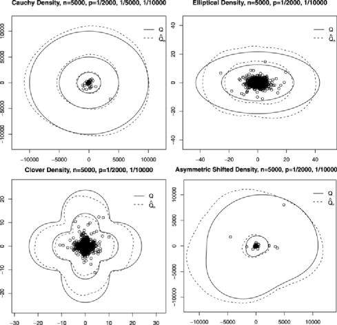
Figure 1: True and estimated risk regions based on one sample of size 5,000 from the bivariate Cauchy distribution, the elliptical distribution in (13), the clover distribution in (14) and the asymmetric shifted distribution in (15).

In addition, we simulated one sample of the bivariate distribution with independent $t_{3}$-components. This distribution does not satisfy condition (a), since the spectral measure is discrete and concentrated on the intersection of the coordinate axes with the unit circle. We also simulated one sample of a bivariate “logarithmic” distribution with $\alpha=1$ and uniform spectral measure, but where the radial distribution satisfies $U(t)/(t\log t)$ tends to a constant and hence $U(t)/t\to\infty$ as $t\to\infty$, that is, this distribution does not satisfy condition (c). Although both distributions do not satisfy our conditions, we see nevertheless satisfactory behavior of the estimator in Figure 2. In the left panel, the estimated region has about the right size and the difficult shape is approximated reasonably well; in the right panel, we see that both the shape and the size are approximated quite well.

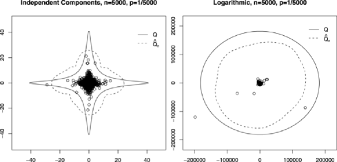
Figure 2: True and estimated risk regions based on one sample of size $5\mbox{,}000$ from the bivariate distribution with independent $t_{3}$-components and the “logarithmic” distribution.

After this visual assessment of our estimator based on one sample at a time, we now investigate its performance based on 100 simulated samples of size 5,000. We will compare our estimator (denoted EVT) to a nonparametric and to a more parametric estimator. The nonparametric estimator is only defined in case $p=1/n$ and tries to mimic the largest order statistic as an estimator of the $(1-1/n)$th quantile in the univariate case. It aims at elliptical level sets. It is defined as follows. First, calculate the smallest ellipsoid containing half of the data, the so-called MVE. Then inflate this ellipsoid, such that the “largest” observation lies on its boundary. Now the region outside this ellipsoid is the estimator.

For $d=2$, the more parametric estimator is defined similarly to $\widehat{Q}_{n}$ in (9), but (only) the estimation of $(\nu(S))^{1/\alpha}S$ is done parametrically. Therefore, this estimator has the same size as $\widehat{Q}_{n}$, but a different shape. (Note that the fully parametric estimator based on multivariate normality would have a very bad performance.) Take the $k$ observations with radius $R_{i}>R_{n-k:n}$ and consider the transformed data $(R_{i}/R_{n-k:n},\mathbf{W}_{i})$. In line with the limit result in (1), assume that these data have a “distribution” $(\cdot)^{-\alpha}\Psi$, where $\Psi$ depends on a parameter $\rho$. To be precise, we assume for the density

$$\psi_{\rho}(\theta)=(4\pi)^{-1}\bigl{(}2+\sin\bigl{(}2(\theta-\rho)\bigr{)}\bigr{)},\qquad 0\leq\theta<2\pi,0\leq\rho<\pi.$$

(Here a point on the unit circle is represented by its angle $\theta\in[0,2\pi)$.) Now $\alpha$ and $\rho$ are estimated by maximum likelihood; observe that this yields the Hill estimator for $1/\alpha$.

=265pt Density EVT p1 Par p1 NP p1 EVT p2 Par p2 Biv. Cauchy $0.28$ $0.29$ $0.72$ $0.31$ $0.32$ Triv. Cauchy $0.22$ – $0.54$ $0.24$ – Elliptical $0.36$ $0.51$ $0.80$ $0.39$ $0.54$ Clover $0.44$ $0.57$ $0.58$ $0.49$ $0.61$ Asymm. shifted $0.26$ $0.27$ $0.61$ $0.30$ $0.32$

Table 1: Median of the relative errors $P(\widehat{Q}_{n}\triangle Q_{n})/p$ of the three estimators, for $p=1/5\mbox{,}000$ (p1) and $1/10\mbox{,}000$ (p2)

Figure 3: Boxplots of ${P(\widehat{Q}_{n}\triangle Q_{n})}/{p}$ for the here proposed estimator and for the parametric and the nonparametric estimator, based on $100$ simulated data sets of size 5,000 from the five presented densities for $p=1/5\mbox{,}000$ (p1) and $1/10\mbox{,}000$ (p2).

Table 1 shows for the three different estimators the median of the 100 relative errors $P(\widehat{Q}_{n}\triangle Q_{n})/p$ for $p=1/5\mbox{,}000$ (p1) and $1/10\mbox{,}000$ (p2). In Figure 3, boxplots are shown of the relative error $P(\widehat{Q}_{n}\triangle Q_{n})/p$ for $p=1/5\mbox{,}000$ (p1) and $1/10\mbox{,}000$ (p2). From this table and figure, we see a good performance of our estimator. Its behavior does not change much if $p$ changes from $1/5\mbox{,}000$ to $1/10\mbox{,}000$. The parametric estimator performs reasonably well, but it is outperformed by our estimator, in particular for the elliptical and clover densities. Recall that this estimator can be seen as a modification of our estimator, since it uses the same estimated inflation factor, but the shape is estimated differently. We see a moderate performance of the nonparametric estimator; also, it cannot be adapted to $p=1/10\mbox{,}000$. Given that the estimation of these extreme risk regions is a statistically difficult problem, we see decent behavior of the three estimation methods. Obviously the parametric and the nonparametric estimator do not perform well if the parametric part of the model is not adequate or if the shape of the region is not elliptical, respectively. The EVT estimator, presented in this paper, does not suffer from these shortcomings and performs well for many multivariate distributions.

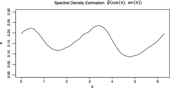
Figure 4: Estimator of $\psi$ of bivariate exchange rate returns.

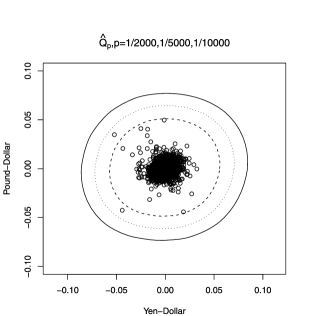
Figure 5: Estimated extreme risk regions of exchange rate returns.

4 Application

In this section, an application of our method to foreign exchange rate data is presented. The data are the daily exchange rates of Yen-Dollar and Pound-Dollar from January 4, 1999 to July 31, 2009. Consider the daily log returns given by $X_{i,j}=\log{({Y_{i+1,j}}/{Y_{i,j}})}$, with $i=1,\ldots,2\mbox{,}664$, $j=1,2$, and $Y_{i,1}$ is the daily exchange rate of the Yen to the Dollar and $Y_{i,2}$ of the Pound to the Dollar. First, we check the equality of the extreme value indices (the reciprocals of the tail indices) of the right and left tails of both marginal distributions and that of the radius. This yields 5 extreme value indices; the 5 estimates in increasing order are: 0.141, 0.191, 0.223, 0.242, 0.256. Hence, the maximal difference is 0.115. Based on the asymptotic normality of the moment estimator of the extreme value index, we compute an approximate upper bound for the maximal difference of the 5 estimators under the null hypothesis of equality: 0.264. Hence, there is no evidence that the 5 extreme value indices are different. Other exchange rate data sets share this property. There are also economic arguments supporting this claim. Therefore, we estimate $\alpha$ based on the radius and find $\widehat{\alpha}=3.90$. As a next step, we estimate the density $\psi$ of the spectral measure. The estimate $\widehat{\psi}_{n}$ is depicted in Figure 4; it is almost periodic with period $\pi$. This yields that the boundary of the estimated extreme risk region is not like a circle, but more like an ellipse. The location of the maxima of $\widehat{\psi}_{n}$ correspond to the major axis of the region. We estimate the extreme risk regions for $p=1/2\mbox{,}000,1/5\mbox{,}000$ and $1/10$,$000$; see Figure 5. For risk management of financial institutions in the U.S., it is important to know which extreme exchange rate returns w.r.t. the Pound and the Yen can occur and which returns essentially never occur. Our estimate answers this question. More specifically, points on the boundary of the estimated extreme risk region can be used as multivariate stress test scenarios. A scenario on the intersection of the major axis of the ellipse-like boundary of the extreme risk region and the boundary itself corresponds to a larger shock than a scenario on the intersection of the minor axis of the ellipse-like boundary and the boundary itself, but our method shows that their “extremeness” is about the same.

5 Proofs

For the proof of the theorem, we need several lemmas and propositions. We assume throughout that the conditions of the theorem are in force. We start with a lemma on regular variation in $\mathbb{R}^{d}$.

Lemma 1

Write $l=1/\int_{\{\|\mathbf{z}\|\geq 1\}}q(\mathbf{z})\,d\mathbf{z}$. For any $\varepsilon>0$,

$$\lim_{t\rightarrow\infty}\sup_{\|\mathbf{z}\|\geq\varepsilon}\biggl{|}\frac{f(t\mathbf{z})}{t^{-d}V(t)}-q(\mathbf{z})\biggr{|}=0.$$ (16)

Moreover

$$\lim_{t\rightarrow\infty}\frac{\mathbb{P}(\mathbf{X}\in tB)}{V(t)}=\int_{B}q(\mathbf{z})\,d\mathbf{z}$$ (17)

for any Borel set $B$ bounded away from the origin. Define $q_{t}(\mathbf{z})=t(U(t))^{d}\times f(U(t)\mathbf{z})$. Then

$$\lim_{t\rightarrow\infty}\sup_{\|\mathbf{z}\|\geq\varepsilon}|q_{t}(\mathbf{z})-lq(\mathbf{z})|=0.$$ (18)

Let $\widetilde{h}$ be the density of $H$, then

$$\lim_{t\rightarrow\infty}\frac{\widetilde{h}(t)}{t^{-1}V(t)}=\frac{\alpha}{l}.$$ (19)

For any $\|\mathbf{z}\|\geq\varepsilon>0$ [cf. Theorem 2.1 in de Haan and Resnick (1987)],

$$\biggl{|}\frac{f(t\mathbf{z})}{t^{-d}V(t)}-q(\mathbf{z})\biggr{|}$$

$$\qquad=\biggl{|}\frac{f(t\|\mathbf{z}\|(\mathbf{z}/{\|\mathbf{z}\|}))}{(t\|z\|)^{-d}V(t\|z\|)}\cdot\frac{(t\|z\|)^{-d}V(t\|z\|)}{t^{-d}V(t)}-q(\mathbf{z})\biggr{|}$$

$$\qquad\leq\|\mathbf{z}\|^{-d-\alpha}\biggl{|}\frac{f(t\|\mathbf{z}\|({\mathbf{z}}/{\|\mathbf{z}\|}))}{(t\|z\|)^{-d}V(t\|z\|)}-q\biggl{(}\frac{\mathbf{z}}{\|\mathbf{z}\|}\biggr{)}\biggr{|}$$

$$\qquad\quad{}+\frac{f(t\|\mathbf{z}\|({\mathbf{z}}/{\|\mathbf{z}\|}))}{(t\|z\|)^{-d}V(t\|z\|)}\biggl{|}\frac{(t\|z\|)^{-d}V(t\|z\|)}{t^{-d}V(t)}-\|\mathbf{z}\|^{-d-\alpha}\biggr{|}$$

Then (16) follows from condition (a).

Let a Borel set $B$ be such that $B\subset\{\|\mathbf{z}\|\geq\gamma\}$, for some $\gamma>0$. Then for $\mathbf{z}\in B$ and sufficiently large $t$, ${f(t\mathbf{z})}/{t^{-d}V(t)}$ is bounded by $q(\|\mathbf{z}\|^{-1}\mathbf{z})\|\mathbf{z}\|^{-a/2-d}$. Hence, (17) holds by Lebesgue’s dominated convergence theorem.

We have from (17), as $t\rightarrow\infty$,

$$tV(U(t))=\frac{V(U(t))}{\mathbb{P}(R\geq U(t))}\rightarrow l.$$

Hence (16) implies, uniformly for $\|\mathbf{z}\|\geq\varepsilon$,

$$q_{t}(\mathbf{z})=tV(U(t))\frac{f(U(t)\mathbf{z})}{(U(t))^{-d}V(U(t))}\rightarrow lq(\mathbf{z}).$$

Note that

$$1-H(t)=\mathbb{P}(R>t)=\int_{t}^{\infty}\int_{\Theta}f(r\mathbf{w})\,d\lambda(\mathbf{w})r^{d-1}\,dr.$$

By taking derivatives, (16) and the homogeneity of $q$, we obtain

$$\lim_{t\rightarrow\infty}\frac{\widetilde{h}(t)}{t^{-1}V(t)}=\int_{\Theta}q(\mathbf{w})\,d\lambda(\mathbf{w})=\alpha\int_{\{\|\mathbf{z}\|\geq 1\}}q(\mathbf{z})\,d\mathbf{z}=\alpha/l.$$

We now see that (5) and (6) hold with $V=1-H$. From now on, we will make the choice $V=1-H$ and hence $l=1$. Note that with this choice the relations (3) [with $\nu(B)=\int_{B}q(\mathbf{z})\,d\mathbf{z}$] and (4) readily follow from (17).

Corollary 1.

For all Borel sets $B$ with positive distance from the origin,

$$\lim_{t\rightarrow\infty}tP(U(t)B)=\nu(B)$$ (20)

and

$$\lim_{n\rightarrow\infty}\frac{\nu(S)}{p}P\biggl{(}U\biggl{(}\frac{n}{k}\biggr{)}\biggl{(}\frac{k\nu(S)}{np}\biggr{)}^{1/{\alpha}}B\biggr{)}=\nu(B).$$ (21)

From $\mathbb{P}(R\geq U(t))=1/t$ and (3), we obtain (20). It follows from (c) that

$$\frac{U({\nu(S)}/{p})}{U({n}/{k})({k\nu(S)}/{(np)})^{{1}/{\alpha}}}\rightarrow 1.$$ (22)

This yields (21).

Lemma 2

For each $\varepsilon>0$, there exists a $\delta>0$ and $t_{0}>0$ such that for $t>t_{0}$

$$\biggl{\{}\mathbf{z}\dvtx\frac{f(t\mathbf{z})}{t^{-d}V(t)}\leq\varepsilon\biggr{\}}\subset\{\mathbf{z}\dvtx\|\mathbf{z}\|>\delta\}.$$

It is sufficient to prove $\{\mathbf{z}\dvtx\|\mathbf{z}\|\leq\delta\}\subset\{\mathbf{z}\dvtx f(t\mathbf{z})/(t^{-d}V(t))>\varepsilon\}$. First, by (6) and the continuity of $q$, for some $c_{1}>0$, there exists $s_{0}>0$ such that for $s>s_{0}$

$$\inf_{\mathbf{w}\in\Theta}\frac{f(s\mathbf{w})}{s^{-d}V(s)}\geq c_{1}$$

and also for $s_{1},s_{2}>s_{0}$ [cf. Proposition B.1.9.5 in de Haan and Ferreira (2006)]

$$\frac{V(s_{1})}{V(s_{2})}>\frac{1}{2}\biggl{(}\frac{s_{1}}{s_{2}}\biggr{)}^{-\alpha/2}.$$

Now for $t>s_{0}$ and any $\mathbf{z}\in\{\mathbf{z}\dvtx\|\mathbf{z}\|\leq\delta\}$, there are two possibilities. [(ii)]

$t\|\mathbf{z}\|>s_{0}$, then

$$\frac{f(t\mathbf{z})}{t^{-d}V(t)}=\frac{f(t\|\mathbf{z}\|(\mathbf{z}/{\|\mathbf{z}\|}))}{(t\|\mathbf{z}\|)^{-d}V(t\|\mathbf{z}\|)}\cdot\frac{(t\|\mathbf{z}\|)^{-d}V(t\|\mathbf{z}\|)}{t^{-d}V(t)}>\frac{1}{2}c_{1}\delta^{-\alpha/2-d}>\varepsilon;$$

$t\|\mathbf{z}\|\leq s_{0}$, then by continuity of $f$ and $f>0$, we have for some $c_{2}>0$, $f(t\mathbf{z})\geq c_{2}$, and hence, since $\lim_{t\to\infty}t^{-d}V(t)=0$, we obtain for $t>t_{0}(\geq s_{0})$

$$\frac{f(t\mathbf{z})}{t^{-d}V(t)}>\varepsilon.$$

Lemma 3

For $\varepsilon>0$ and large $n$,

$$\bar{Q}_{n}\subset U\biggl{(}\frac{\nu(S)}{p}\biggr{)}\{\mathbf{z}\dvtx q(\mathbf{z})\leq 1+\varepsilon\}$$

and

$$\bar{Q}_{n}\supset U\biggl{(}\frac{\nu(S)}{p}\biggr{)}\{\mathbf{z}\dvtx q(\mathbf{z})\leq 1-\varepsilon\}.$$

Recall that $\bar{Q}_{n}=\{\mathbf{z}\dvtx f(\mathbf{z})\leq(\frac{np}{k\nu(S)})^{1+({d}/{\alpha})}\frac{1}{({n}/{k})(U({n}/{k}))^{d}}\}$. It follows from (22) that for $n$ large enough and $\varepsilon_{1}>0$

$$\bar{Q}_{n} = U\biggl{(}\frac{\nu(S)}{p}\biggr{)}\biggl{\{}\mathbf{z}\dvtx f\biggl{(}U\biggl{(}\frac{\nu(S)}{p}\biggr{)}\mathbf{z}\biggr{)}\leq\biggl{(}\frac{np}{k\nu(S)}\biggr{)}^{1+({d}/{\alpha})}\frac{1}{({n}/{k})(U({n}/{k}))^{d}}\biggr{\}}$$

$$= U\biggl{(}\frac{\nu(S)}{p}\biggr{)}\biggl{\{}\mathbf{z}\dvtx q_{\nu(S)/p}(\mathbf{z})\leq\biggl{(}\frac{np}{k\nu(S)}\biggr{)}^{{d}/{\alpha}}\biggl{(}U\biggl{(}\frac{n}{k}\biggr{)}\biggr{)}^{-d}\biggl{(}U\biggl{(}\frac{\nu(S)}{p}\biggr{)}\biggr{)}^{d}\biggr{\}}$$

$$\subset U\biggl{(}\frac{\nu(S)}{p}\biggr{)}\bigl{\{}\mathbf{z}\dvtx q_{\nu(S)/p}(\mathbf{z})\leq 1+\varepsilon_{1}\bigr{\}}.$$

Now Lemma 2 implies $\{\mathbf{z}\dvtx q_{\nu(S)/p}(\mathbf{z})\leq 1+\varepsilon_{1}\}\subset\{\mathbf{z}\dvtx\|\mathbf{z}\|>\delta\}$, hence we have by (18)

$$\bar{Q}_{n}\subset U\biggl{(}\frac{\nu(S)}{p}\biggr{)}\{\mathbf{z}\dvtx q(\mathbf{z})\leq 1+\varepsilon\}.$$

The other inclusion follows in the same way (but Lemma 2 is not needed).

Lemma 4

For $\varepsilon>0$ and large $n$,

$$\widetilde{Q}_{n}\subset U\biggl{(}\frac{\nu(S)}{p}\biggr{)}\{\mathbf{z}\dvtx q(\mathbf{z})\leq 1+\varepsilon\}$$

and

$$\widetilde{Q}_{n}\supset U\biggl{(}\frac{\nu(S)}{p}\biggr{)}\{\mathbf{z}\dvtx q(\mathbf{z})\leq 1-\varepsilon\}.$$

Recall that $\widetilde{Q}_{n}=U(\frac{n}{k})(\frac{k\nu(S)}{np})^{{1}/{\alpha}}\{\mathbf{z}\dvtx q(z)\leq 1\}$.

Put $T_{n}=(U(\frac{\nu(S)}{p}))^{-1}U(\frac{n}{k})(\frac{k\nu(S)}{np})^{{1}/{\alpha}}$, then

$$\widetilde{Q}_{n} = U\biggl{(}\frac{\nu(S)}{p}\biggr{)}\{T_{n}\mathbf{z}\dvtx q(\mathbf{z})\leq 1\}=U\biggl{(}\frac{\nu(S)}{p}\biggr{)}\{T_{n}\mathbf{z}\dvtx q(T_{n}\mathbf{z})\leq T_{n}^{-d-\alpha}\}$$

$$= U\biggl{(}\frac{\nu(S)}{p}\biggr{)}\{\mathbf{z}\dvtx q(\mathbf{z})\leq T_{n}^{-d-\alpha}\}.$$

Since $T_{n}\rightarrow 1$ as $n\rightarrow\infty$ by (22), the result follows.

Proposition 1

We have

$$\lim_{n\rightarrow\infty}\frac{P(Q_{n}\bigtriangleup\widetilde{Q}_{n})}{p}=0.$$

Note that $P(Q_{n}\bigtriangleup\widetilde{Q}_{n})\leq P(Q_{n}\bigtriangleup\bar{Q}_{n})+P(\bar{Q}_{n}\bigtriangleup\widetilde{Q}_{n})$. Observe that $Q_{n}\subset\bar{Q}_{n}$ or $\bar{Q}_{n}\subset Q_{n}$, hence $P(Q_{n}\bigtriangleup\bar{Q}_{n})\leq|p-P(\bar{Q}_{n})|$. By Lemma 3 and Corollary 1, for any $\varepsilon>0$ and large $n$

$$\frac{\nu(S)}{p}P(\bar{Q}_{n}) \leq \frac{\nu(S)}{p}P\biggl{(}U\biggl{(}\frac{\nu(S)}{p}\biggr{)}\{\mathbf{z}\dvtx q(\mathbf{z})\leq 1+\varepsilon\}\biggr{)}$$

$$\rightarrow \nu\bigl{(}\{\mathbf{z}\dvtx q(\mathbf{z})\leq 1+\varepsilon\}\bigr{)}$$

$$= \nu\bigl{(}\bigl{\{}\mathbf{z}\dvtx q\bigl{(}\mathbf{z}(1+\varepsilon)^{1/(d+\alpha)}\bigr{)}\leq 1\bigr{\}}\bigr{)}$$

$$= \nu\bigl{(}\bigl{\{}(1+\varepsilon)^{-1/(d+\alpha)}\mathbf{z}\dvtx q(\mathbf{z})\leq 1\bigr{\}}\bigr{)}$$

$$= (1+\varepsilon)^{\alpha/(d+\alpha)}\nu(S).$$

Thus, $\limsup_{n\rightarrow\infty}\frac{P(\bar{Q}_{n})}{p}\leq(1+\varepsilon)^{\alpha/(2+\alpha)}$.

Similarly, we have $\liminf_{n\rightarrow\infty}\frac{P(\bar{Q}_{n})}{p}\geq(1-\varepsilon)^{\alpha/(2+\alpha)}$. Hence,$\lim_{n\rightarrow\infty}\frac{P(\bar{Q}_{n})}{p}=1$, that is, $\lim_{n\rightarrow\infty}\frac{P(Q_{n}\bigtriangleup\bar{Q}_{n})}{p}=0$.

In the same way, it follows from Lemmas 3 and 4 that

$$\frac{\nu(S)}{p}P(\bar{Q}_{n}\bigtriangleup\widetilde{Q}_{n}) \leq \frac{\nu(S)}{p}P\biggl{(}U\biggl{(}\frac{\nu(S)}{p}\biggr{)}\{\mathbf{z}\dvtx 1-\varepsilon\leq q(\mathbf{z})\leq 1+\varepsilon\}\biggr{)}$$

$$\rightarrow \nu\bigl{(}\{\mathbf{z}\dvtx 1-\varepsilon\leq q(\mathbf{z})\leq 1+\varepsilon\}\bigr{)}$$

$$= \nu(S)\bigl{(}(1+\varepsilon)^{\alpha/(d+\alpha)}-(1-\varepsilon)^{\alpha/(d+\alpha)}\bigr{)}.$$

Hence, $\lim_{n\rightarrow\infty}\frac{P(\bar{Q}_{n}\bigtriangleup\widetilde{Q}_{n})}{p}=0$.

The following proposition shows uniform consistency of $\widehat{\psi}_{n}$ and might be of independent interest. There is an abundant literature on density estimation for directional data. In particular, uniform consistency of density estimators for directional data has been established in Bai, Rao and Zhao (1988). Here, however, the data do not have a fixed probability density on $\Theta$: the density $\psi$ is defined via a limit relation. Hence, $\psi$ is only an approximate model for the directional data. As a consequence, a more general result is required.

Proposition 2

As $n\rightarrow\infty$,

$$\sup_{\mathbf{w}\in\Theta}|\widehat{\psi}_{n}(\mathbf{w})-\psi(\mathbf{w})|\stackrel{{\scriptstyle\mathbb{P}}}{{\rightarrow}}0.$$

It is easy to see that, for any $\eta>0$, there exists a function

$$K^{*}=\sum_{j=1}^{m}\alpha_{j}1_{[r_{j-1},r_{j})}$$

with $1\geq\alpha_{1}\geq\alpha_{2}\geq\cdots\geq\alpha_{m}\geq 0$ and $0=r_{0}<r_{1}<\cdots<r_{m}=1$, such that

$$\sup_{u\in[0,1]}|K(u)-K^{*}(u)|\leq\eta.$$

Write $U_{i}=1-H(R_{i})$, $i=1,\ldots,n$, and denote the corresponding order statistics with $U_{i:n}$. Let $\widetilde{P}$ be the probability measure on $\Theta\times(0,1)$ corresponding to $(\mathbf{W}_{1},U_{1})$ and let $\widetilde{P}_{n}$ be the empirical measure of the $(\mathbf{W}_{i},U_{i})$ $i=1,\ldots,n$. Define

$$\psi_{n}^{*}(\mathbf{w})=\frac{c(h,K)}{k}\sum_{i=1}^{n}K^{*}\biggl{(}\frac{1-\mathbf{w}^{T}\mathbf{W}_{i}}{h}\biggr{)}1_{[R_{i}>R_{n-k:n}]}$$

and

$$\psi_{n,j}^{*}(\mathbf{w})=\frac{nc(h,K)}{k}\widetilde{P}_{n}\bigl{(}D_{\mathbf{w},j}\times(0,U_{k:n}]\bigr{)}$$

with $D_{\mathbf{w},j}=\{\mathbf{v}\in\Theta\dvtx 1-hr_{j}<\mathbf{w}^{T}\mathbf{v}\leq 1-hr_{j-1}\}$. Observe that $\psi_{n}^{*}(\mathbf{w})=\sum_{j=1}^{m}\alpha_{j}\psi_{n,j}^{*}(\mathbf{w})$. Also write

$$\psi_{n,j}(\mathbf{w})=\frac{nc(h,K)}{k}\widetilde{P}\bigl{(}D_{\mathbf{w},j}\times(0,U_{k:n}]\bigr{)}.$$

Let $\varepsilon>0$. It is sufficient to show that for large $n$

$$\mathbb{P}\Biggl{(}\sup_{\mathbf{w}\in\Theta}\Biggl{|}\widehat{\psi}_{n}(\mathbf{w})-\sum_{j=1}^{m}\alpha_{j}\psi_{n,j}(\mathbf{w})\Biggr{|}\geq 2\varepsilon\Biggr{)} \leq 2\varepsilon,$$ (23)

$$\mathbb{P}\Biggl{(}\sup_{\mathbf{w}\in\Theta}\Biggl{|}\sum_{j=1}^{m}\alpha_{j}\bigl{(}\psi_{n,j}(\mathbf{w})-c(h,K)\Psi(D_{\mathbf{w},j})\bigr{)}\Biggr{|}\geq 2\varepsilon\Biggr{)} \leq \varepsilon,$$ (24)

$$\sup_{\mathbf{w}\in\Theta}\Biggl{|}c(h,K)\sum_{j=1}^{m}\alpha_{j}\Psi(D_{\mathbf{w},j})-\psi(\mathbf{w})\Biggr{|} \leq \varepsilon.$$ (25)

For $\mathbf{w}\in\Theta$ and $\delta\in(0,1)$, write $\mathcal{C}_{\delta}=\{C_{\mathbf{w}}(a)\dvtx\mathbf{w}\in\Theta,a\leq\delta\}$. Note that, as $n\rightarrow\infty$,

$$\sup_{C\in\mathcal{C}_{1},0<s\leq 2}\frac{1}{\lambda(C)}\biggl{|}\frac{n}{k}\widetilde{P}\bigl{(}C\times(0,sk/n]\bigr{)}-s\Psi(C)\biggr{|}\rightarrow 0.$$ (26)

This readily follows from

$$\frac{n}{k}\widetilde{P}\bigl{(}C\times(0,sk/n]\bigr{)} = \frac{n}{k}\mathbb{P}\biggl{(}\mathbf{W}\in C,R\geq U\biggl{(}\frac{n}{sk}\biggr{)}\biggr{)}$$

$$= \frac{n}{k}\int_{U({n}/{(sk)})}^{\infty}\int_{C}\frac{f(r\mathbf{w})}{r^{-d}V(r)}\,d\lambda(\mathbf{w})\,r^{-1}V(r)\,dr$$

and (16) and (19).

Now we prove (23). It is easy to show that

$$c(h,K)=\biggl{(}\frac{2\pi^{{(d-1)}/{2}}}{\Gamma({(d-1)}/{2})}\int_{1-h}^{1}K\biggl{(}\frac{1-t}{h}\biggr{)}(1-t^{2})^{{(d-3)}/{2}}\,dt\biggr{)}^{-1}$$

and hence

$$\limsup_{h\downarrow 0}c(h,K)\lambda(C_{\mathbf{w}}(h))<\infty.$$ (27)

We have

$$|\widehat{\psi}_{n}(\mathbf{w})-\psi_{n}^{*}(\mathbf{w})|$$

$$\qquad=\frac{c(h,K)}{k}\Biggl{|}\sum_{i=1}^{n}\biggl{(}K\biggl{(}\frac{1-\mathbf{w}^{T}\mathbf{W}_{i}}{h}\biggr{)}-K^{*}\biggl{(}\frac{1-\mathbf{w}^{T}\mathbf{W}_{i}}{h}\biggr{)}\biggr{)}1_{[R_{i}>R_{n-k:n}]}\Biggr{|}$$

$$\qquad\leq\frac{c(h,K)}{k}\sum_{i=1}^{n}\eta 1_{[\mathbf{W}_{i}\in C_{\mathbf{w}}(h),R_{i}>R_{n-k:n}]}$$ (28)

$$\qquad\leq\eta\frac{nc(h,K)}{k}\widetilde{P}\bigl{(}C_{\mathbf{w}}(h)\times(0,U_{k:n}]\bigr{)}$$

$$\qquad\quad{}+\eta\frac{nc(h,K)}{k}\bigl{|}(\widetilde{P}_{n}-\widetilde{P})\bigl{(}C_{\mathbf{w}}(h)\times(0,U_{k:n}]\bigr{)}\bigr{|}.$$

By (26), for $\eta$ small enough the first term is less than $\varepsilon$, with probability tending to one, uniformly in $\mathbf{w}\in\Theta$. Also,

$$\Biggl{|}\psi_{n}^{*}(\mathbf{w})-\sum_{j=1}^{m}\alpha_{j}\psi_{n,j}(\mathbf{w})\Biggr{|}$$

$$\qquad\leq\sum_{j=1}^{m}\alpha_{j}|\psi_{n,j}^{*}(\mathbf{w})-\psi_{n,j}(\mathbf{w})|$$ (29)

$$\qquad\leq\sum_{j=1}^{m}\alpha_{j}\frac{nc(h,K)}{k}\bigl{|}(\widetilde{P}_{n}-\widetilde{P})\bigl{(}D_{\mathbf{w},j}\times(0,U_{k:n}]\bigr{)}\bigr{|}.$$

From (5), (5) and (27), we see that for a proof of (23) it remains to show that

$$\frac{n}{k\lambda(C_{\mathbf{w}}(h))}\sup_{\mathbf{w}\in\Theta}\sup_{0<a\leq 1}\bigl{|}(\widetilde{P}_{n}-\widetilde{P})\bigl{(}C_{\mathbf{w}}(ah)\times(0,U_{k:n}]\bigr{)}\bigr{|}\stackrel{{\scriptstyle\mathbb{P}}}{{\rightarrow}}0.$$

It can be shown that there exists a constant $c=c(d)$ and finitely many $\mathbf{w}_{l}$, $l=1,\ldots,l_{h}$ such that $l_{h}=O(c(h,K))$ as $h\downarrow 0$, and for every $\mathbf{w}\in\Theta$ and $0<a\leq 1$

$$C_{\mathbf{w}}(ah)\in C_{\mathbf{w}_{l}}(ch)\qquad\mbox{for some }l.$$

Hence for $\varepsilon_{1}>0$,

$$\mathbb{P}\biggl{(}\frac{n}{k\lambda(C_{\mathbf{w}}(h))}\sup_{\mathbf{w}\in\Theta}\sup_{0<a\leq 1}\bigl{|}(\widetilde{P}_{n}-\widetilde{P})\bigl{(}C_{\mathbf{w}}(ah)\times(0,U_{k:n}]\bigr{)}\bigr{|}\geq\varepsilon_{1}\biggr{)}$$

$$\qquad\leq\mathbb{P}\Bigl{(}\max_{1\leq l\leq l_{h}}\mathop{\sup_{C\subset C_{\mathbf{w}_{l}}(ch)}}_{C\in\mathcal{C}_{h}}\sup_{0<s\leq 2}\bigl{|}(\widetilde{P}_{n}-\widetilde{P})\bigl{(}C\times(0,sk/n]\bigr{)}\bigr{|}\geq\varepsilon_{1}k/n\lambda(C_{\mathbf{w}}(h))\Bigr{)}$$

$$\qquad\quad{}+\mathbb{P}(U_{k:n}>2k/n)$$

$$\qquad\leq\sum_{l=1}^{l_{h}}\mathbb{P}\Bigl{(}\mathop{\sup_{C\subset C_{\mathbf{w}_{l}}(ch)}}_{C\in\mathcal{C}_{h}}\sup_{0<s\leq 2}\bigl{|}(\widetilde{P}_{n}-\widetilde{P})\bigl{(}C\times(0,sk/n]\bigr{)}\bigr{|}\geq\varepsilon_{1}k/n\lambda(C_{\mathbf{w}}(h))\Bigr{)}$$

$$\qquad\quad{}+\mathbb{P}(U_{k:n}>2k/n).$$

The latter probability tends to $0$, so it suffices to consider the sum of the $l_{h}$ probabilities. Write $b=\varepsilon_{1}k\lambda(C_{\mathbf{w}}(h))$. Fix $l$ and define $N=n\widetilde{P}_{n}(C_{\mathbf{w}_{l}}(ch)\times(0,2k/n])$, $\mu=n\widetilde{P}(C_{\mathbf{w}_{l}}(ch)\times(0,2k/n])$. Define the conditional probability measure $\widetilde{P}_{c}=\frac{n\widetilde{P}}{\mu}$ on $C_{\mathbf{w}_{l}}(ch)\times(0,2k/n]$ and let $\widetilde{P}_{c,r}$ be the corresponding empirical measure, based on $r$ observations. We have

$$\mathbb{P}\Bigl{(}\mathop{\sup_{C\subset C_{\mathbf{w}_{l}}(ch)}}_{C\in\mathcal{C}_{h}}\sup_{0<s\leq 2}n\bigl{|}(\widetilde{P}_{n}-\widetilde{P})\bigl{(}C\times(0,sk/n]\bigr{)}\bigr{|}\geq b\Bigr{)}$$

$$\qquad\leq\sum_{r=\lceil\mu-b/3\rceil}^{r=\lfloor\mu+b/3\rfloor}\mathbb{P}\Bigl{(}\mathop{\sup_{C\subset C_{\mathbf{w}_{l}}(ch)}}_{C\in\mathcal{C}_{h}}\sup_{0<s\leq 2}n\bigl{|}(\widetilde{P}_{n}-\widetilde{P})\bigl{(}C\times(0,sk/n]\bigr{)}\bigr{|}\geq b\big{|}N=r\Bigr{)}$$

$$\qquad\quad\hphantom{\sum_{r=\lceil\mu-b/3\rceil}^{r=\lfloor\mu+b/3\rfloor}}{}\times\mathbb{P}(N=r)+\mathbb{P}(|N-\mu|\geq b/3)$$

$$\qquad\leq\sum_{r=\lceil\mu-b/3\rceil}^{r=\lfloor\mu+b/3\rfloor}\mathbb{P}\biggl{(}\mathop{\sup_{C\subset C_{\mathbf{w}_{l}}(ch)}}_{C\in\mathcal{C}_{h}}\sup_{0<s\leq 2}n\biggl{|}\biggl{(}\widetilde{P}_{n}-\frac{N}{\mu}\widetilde{P}\biggr{)}\bigl{(}C\times(0,sk/n]\bigr{)}\biggr{|}$$

$$\hskip 252.0pt\geq\frac{b}{2}\Big{|}N=r\biggr{)}\mathbb{P}(N=r)$$

$$\qquad\quad{}+\sum_{r=\lceil\mu-b/3\rceil}^{r=\lfloor\mu+b/3\rfloor}\mathbb{P}\biggl{(}\mathop{\sup_{C\subset C_{\mathbf{w}_{l}}(ch)}}_{C\in\mathcal{C}_{h}}\sup_{0<s\leq 2}n\biggl{|}\frac{(N-\mu)}{\mu}\widetilde{P}\bigl{(}C\times(0,sk/n]\bigr{)}\biggr{|}$$

$$\hskip 255.0pt\geq\frac{b}{2}\Big{|}N=r\biggr{)}\mathbb{P}(N=r)$$

$$\qquad\quad{}+\mathbb{P}(|N-\mu|\geq b/3)$$ (30)

$$\qquad\leq\sum_{r=\lceil\mu-b/3\rceil}^{r=\lfloor\mu+b/3\rfloor}\mathbb{P}\biggl{(}\mathop{\sup_{C\subset C_{\mathbf{w}_{l}}(ch)}}_{C\in\mathcal{C}_{h}}\sup_{0<s\leq 2}r\bigl{|}(\widetilde{P}_{c,r}-\widetilde{P}_{c})\bigl{(}C\times(0,sk/n]\bigr{)}\bigr{|}\geq\frac{b}{2}\biggr{)}$$

$$\qquad\quad\hphantom{\sum_{r=\lceil\mu-b/3\rceil}^{r=\lfloor\mu+b/3\rfloor}}{}\times\mathbb{P}(N=r)$$

$$\qquad\quad{}+\sum_{r=\lceil\mu-b/3\rceil}^{r=\lfloor\mu+b/3\rfloor}\mathbb{P}\biggl{(}|r-\mu|\geq\frac{b}{2}\biggr{)}\mathbb{P}(N=r)+\mathbb{P}(|N-\mu|\geq b/3).$$

Note that the first probability of the second sum in the right side of (5) is equal to 0. From Bennett’s inequality [cf. Shorack and Wellner (1986), page 851], it follows that for some constant $c_{1}$

$$\mathbb{P}(|N-\mu|\geq b/3)\leq 2\exp\biggl{(}-\varepsilon_{1}^{2}c_{1}\frac{k}{c(h,K)}\biggr{)}.$$

Hence, since $l_{h}=O(c(h,K))$,

$$\sum_{l=1}^{l_{h}}\mathbb{P}(|N-\mu|\geq b/3)=O\biggl{(}c(h,K)\exp\biggl{(}-\varepsilon_{1}^{2}c_{1}\frac{k}{c(h,K)}\biggr{)}\biggr{)}=o(1).$$

To complete the proof of (23), we need to consider the first sum in the right side of (5). For the first probability in there, we use Corollary 2.9 in Alexander (1984), a good probability bound for empirical processes on VC classes. We obtain as an upper bound

$$16\exp\biggl{(}-\frac{b^{2}}{4r}\biggr{)}.$$

Using $r\leq\mu+b/3$, we find for some constant $c_{2}$

$$\sum_{l=1}^{l_{h}}\sum_{r=\lceil\mu-b/3\rceil}^{r=\lfloor\mu+b/3\rfloor}\mathbb{P}\biggl{(}\mathop{\sup_{C\subset C_{\mathbf{w}_{l}}(ch)}}_{C\in\mathcal{C}_{h}}\sup_{0<s\leq 2}r\bigl{|}(\widetilde{P}_{c,r}-\widetilde{P}_{c})\bigl{(}C\times(0,sk/n]\bigr{)}\bigr{|}\geq\frac{b}{2}\biggr{)}$$

$$\hphantom{\sum_{l=1}^{l_{h}}\sum_{r=\lceil\mu-b/3\rceil}^{r=\lfloor\mu+b/3\rfloor}}{}\times\mathbb{P}(N=r)$$

$$\qquad\leq 16\sum_{l=1}^{l_{h}}\sum_{r=\lceil\mu-b/3\rceil}^{r=\lfloor\mu+b/3\rfloor}\exp\biggl{(}-\varepsilon_{1}^{2}c_{2}\frac{k}{c(h,K)}\biggr{)}\mathbb{P}(N=r)$$

$$\qquad\leq 16\sum_{l=1}^{l_{h}}\exp\biggl{(}-\varepsilon_{1}^{2}c_{2}\frac{k}{c(h,K)}\biggr{)}$$

$$\qquad=o(1).$$

Next, we show (24). From (27) and (26), we obtain for $\varepsilon_{2}>0$ small enough,

$$\sup_{\mathbf{w}\in\Theta}\Biggl{|}\sum_{j=1}^{m}\alpha_{j}\bigl{(}\psi_{n,j}(\mathbf{w})-c(h,K)\Psi(D_{\mathbf{w},j})\bigr{)}\Biggr{|}$$

$$\qquad=\sup_{\mathbf{w}\in\Theta}\Biggl{|}\sum_{j=1}^{m}\alpha_{j}c(h,K)\bigl{(}n/k\widetilde{P}\bigl{(}D_{\mathbf{w},j}\times(0,U_{k:n}]\bigr{)}-\Psi(D_{\mathbf{w},j})\bigr{)}\Biggr{|}$$

$$\qquad\leq\varepsilon_{2}\sum_{j=1}^{m}\alpha_{j}c(h,K)\lambda(C_{\mathbf{w}}(h))+\sup_{\mathbf{w}\in\Theta}\Biggl{|}\sum_{j=1}^{m}\alpha_{j}c(h,K)(nU_{k:n}/k-1)\Psi(D_{\mathbf{w},j})\Biggr{|}$$

$$\qquad\leq\varepsilon+\biggl{|}\frac{n}{k}U_{k:n}-1\biggr{|}\sum_{j=1}^{m}\alpha_{j}c(h,K)\lambda(C_{\mathbf{w}}(h))\sup_{\mathbf{w}\in\Theta}\psi(\mathbf{w})<2\varepsilon$$

with probability tending to one.

It remains to prove (25). It is readily seen that $\int_{C_{\mathbf{w}}(h)}K^{*}(\frac{1-\mathbf{w}^{T}\mathbf{v}}{h})\,d\lambda(\mathbf{v})=\sum_{j=1}^{m}\alpha_{j}\lambda(D_{\mathbf{w},j})$. Hence, for $\varepsilon_{3}>0$ small enough

$$\sup_{\mathbf{w}\in\Theta}\Biggl{|}c(h,K)\sum_{j=1}^{m}\alpha_{j}\Psi(D_{\mathbf{w},j})-\psi(\mathbf{w})\Biggr{|}$$

$$\qquad\leq\sup_{\mathbf{w}\in\Theta}\psi(\mathbf{w})\Biggl{|}c(h,K)\sum_{j=1}^{m}\alpha_{j}\lambda(D_{\mathbf{w},j})-1\Biggr{|}+\varepsilon_{3}c(h,K)\sum_{j=1}^{m}\alpha_{j}\lambda(D_{\mathbf{w},j})$$

$$\qquad\leq\sup_{\mathbf{w}\in\Theta}\psi(\mathbf{w})\biggl{|}\frac{\int_{C_{\mathbf{w}}(h)}K^{*}({(1-\mathbf{w}^{T}\mathbf{v})}/{h})\,d\lambda(\mathbf{v})}{\int_{C_{\mathbf{w}}(h)}K({(1-\mathbf{w}^{T}\mathbf{v})}/{h})\,d\lambda(\mathbf{v})}-1\biggr{|}$$

$$\qquad\quad{}+\varepsilon_{3}c(h,K)\lambda(C_{\mathbf{w}}(h))\sum_{j=1}^{m}\alpha_{j}$$

$$\qquad\leq\eta c(h,K)\lambda(C_{\mathbf{w}}(h))\sup_{\mathbf{w}\in\Theta}\psi(\mathbf{w})+\varepsilon_{3}c(h,K)\lambda(C_{\mathbf{w}}(h))\sum_{j=1}^{m}\alpha_{j}$$

$$\qquad\leq\varepsilon.$$

From Proposition 2 and the consistency of $\widehat{\alpha}$, we obtain immediately, as $n\rightarrow\infty$,

$$\widehat{\nu(S)}\stackrel{{\scriptstyle\mathbb{P}}}{{\rightarrow}}\nu(S)$$

and, for $\varepsilon>0$,

$$\mathbb{P}\bigl{(}(1+\varepsilon)S\subset\widehat{S}\subset(1-\varepsilon)S\bigr{)}\to 1.$$ (31)

Proposition 3

As $n\rightarrow\infty$,

$$\frac{P(\widetilde{Q}_{n}\triangle\widehat{Q}_{n})}{p}\stackrel{{\scriptstyle\mathbb{P}}}{{\rightarrow}}0.$$

Note that as $n\rightarrow\infty$, we have

$$\widehat{U}\biggl{(}\frac{n}{k}\biggr{)}\Big{/}U\biggl{(}\frac{n}{k}\biggr{)} \stackrel{{\scriptstyle\mathbb{P}}}{{\rightarrow}} 1,$$

$$(\widehat{\nu(S)})^{{1}/{\widehat{\alpha}}} \stackrel{{\scriptstyle\mathbb{P}}}{{\rightarrow}} (\nu(S))^{1/\alpha},$$

$$\biggl{(}\frac{k}{np}\biggr{)}^{1/\widehat{\alpha}-1/\alpha} = \exp\biggl{(}\frac{\sqrt{k}(\alpha-\widehat{\alpha})}{\widehat{\alpha}\alpha}\biggl{(}\frac{\log k}{\sqrt{k}}-\frac{\log(np)}{\sqrt{k}}\biggr{)}\biggr{)}\stackrel{{\scriptstyle\mathbb{P}}}{{\rightarrow}}1.$$

Combining these three limit relations, we obtain

$$\frac{\widehat{U}({n}/{k})({k\widehat{\nu(S)}}/{(np)})^{{1}/{\widehat{\alpha}}}}{U({n}/{k})({k\nu(S)}/{(np)})^{{1}/{\alpha}}}\stackrel{{\scriptstyle\mathbb{P}}}{{\rightarrow}}1.$$

This and (31) yields that with probability tending to one, as $n\to\infty$,

$$(1+\varepsilon)^{2}\widetilde{Q}_{n}\subset\widehat{Q}_{n}\subset(1-\varepsilon)^{2}\widetilde{Q}_{n}.$$

Then,

$$\frac{P(\widetilde{Q}_{n}\triangle\widehat{Q}_{n})}{p}\leq\frac{1}{p}P\biggl{(}U\biggl{(}\frac{n}{k}\biggr{)}\biggl{(}\frac{k\nu(S)}{np}\biggr{)}^{{1}/{\alpha}}\bigl{(}(1-\varepsilon)^{2}S\setminus(1+\varepsilon)^{2}S\bigr{)}\biggr{)},$$

and, by (21), the latter expression tends to

$$\nu\bigl{(}(1-\varepsilon)^{2}S\setminus(1+\varepsilon)^{2}S\bigr{)}/\nu(S)$$

$$\qquad=\nu\bigl{(}(1-\varepsilon)^{2}S\bigr{)}/\nu(S)-\nu\bigl{(}(1+\varepsilon)^{2}S\bigr{)}/\nu(S)$$

$$\qquad=(1-\varepsilon)^{-2\alpha}-(1+\varepsilon)^{-2\alpha},$$

which in turn tends to 0, as $\varepsilon\downarrow 0$.

Proof of Theorem 1 The result follows from Propositions 1 and 3.

References

Alexander (1984){barticle}[mr]
\bauthor\bsnmAlexander, \bfnmKenneth S.\binitsK. S.
(\byear1984).
\btitleProbability inequalities for empirical processes and a law of the
iterated logarithm.
\bjournalAnn. Probab.
\bvolume12
\bpages1041–1067.
\bnote[Corr.: 15 (1987) 428–430.]
\bidissn=0091-1798, mr=0757769
\bptnotecheck related
\endbibitem
Bai, Rao and Zhao (1988){barticle}[mr]
\bauthor\bsnmBai, \bfnmZ. D.\binitsZ. D.,
\bauthor\bsnmRao, \bfnmC. Radhakrishna\binitsC. R. and \bauthor\bsnmZhao, \bfnmL. C.\binitsL. C.
(\byear1988).
\btitleKernel estimators of density function of directional data.
\bjournalJ. Multivariate Anal.
\bvolume27
\bpages24–39.
\biddoi=10.1016/0047-259X(88)90113-3, issn=0047-259X, mr=0971170
\endbibitem
Baíllo, Cuesta-Albertos and
Cuevas (2001){barticle}[mr]
\bauthor\bsnmBaíllo, \bfnmAmparo\binitsA.,
\bauthor\bsnmCuesta-Albertos, \bfnmJuan A.\binitsJ. A. and \bauthor\bsnmCuevas, \bfnmAntonio\binitsA.
(\byear2001).
\btitleConvergence rates in nonparametric estimation of level sets.
\bjournalStatist. Probab. Lett.
\bvolume53
\bpages27–35.
\biddoi=10.1016/S0167-7152(01)00006-2, issn=0167-7152, mr=1843338
\endbibitem
Danielsson et al. (2001){barticle}[mr]
\bauthor\bsnmDanielsson, \bfnmJ.\binitsJ., \bauthor\bparticlede
\bsnmHaan, \bfnmL.\binitsL.,
\bauthor\bsnmPeng, \bfnmL.\binitsL. and \bauthor\bparticlede
\bsnmVries, \bfnmC. G.\binitsC. G.
(\byear2001).
\btitleUsing a bootstrap method to choose the sample fraction in tail index
estimation.
\bjournalJ. Multivariate Anal.
\bvolume76
\bpages226–248.
\biddoi=10.1006/jmva.2000.1903, issn=0047-259X, mr=1821820
\endbibitem
de Haan and Ferreira (2006){bbook}[mr]
\bauthor\bparticlede \bsnmHaan, \bfnmLaurens\binitsL.
and \bauthor\bsnmFerreira, \bfnmAna\binitsA.
(\byear2006).
\btitleExtreme Value Theory: An Introduction.
\bpublisherSpringer, \baddressNew York.
\bidmr=2234156
\endbibitem
de Haan and Resnick (1987){barticle}[mr]
\bauthor\bparticlede \bsnmHaan, \bfnmL.\binitsL. and \bauthor\bsnmResnick, \bfnmS.\binitsS.
(\byear1987).
\btitleOn regular variation of probability densities.
\bjournalStochastic Process. Appl.
\bvolume25
\bpages83–93.
\biddoi=10.1016/0304-4149(87)90191-8, issn=0304-4149, mr=0904266
\endbibitem
Dekkers, Einmahl and
de Haan (1989){barticle}[mr]
\bauthor\bsnmDekkers, \bfnmA. L. M.\binitsA. L. M.,
\bauthor\bsnmEinmahl, \bfnmJ. H. J.\binitsJ. H. J. and \bauthor\bparticlede \bsnmHaan, \bfnmL.\binitsL.
(\byear1989).
\btitleA moment estimator for the index of an extreme-value distribution.
\bjournalAnn. Statist.
\bvolume17
\bpages1833–1855.
\biddoi=10.1214/aos/1176347397, issn=0090-5364, mr=1026315
\endbibitem
Einmahl, Li and Liu (2009){barticle}[mr]
\bauthor\bsnmEinmahl, \bfnmJohn H. J.\binitsJ. H. J.,
\bauthor\bsnmLi, \bfnmJun\binitsJ. and \bauthor\bsnmLiu, \bfnmRegina Y.\binitsR. Y.
(\byear2009).
\btitleThresholding events of extreme in simultaneous monitoring of multiple
risks.
\bjournalJ. Amer. Statist. Assoc.
\bvolume104
\bpages982–992.
\biddoi=10.1198/jasa.2009.ap08329, issn=0162-1459, mr=2562001
\endbibitem
Hall, Watson and
Cabrera (1987){barticle}[mr]
\bauthor\bsnmHall, \bfnmPeter\binitsP.,
\bauthor\bsnmWatson, \bfnmG. S.\binitsG. S. and \bauthor\bsnmCabrera, \bfnmJavier\binitsJ.
(\byear1987).
\btitleKernel density estimation with spherical data.
\bjournalBiometrika
\bvolume74
\bpages751–762.
\biddoi=10.1093/biomet/74.4.751, issn=0006-3444, mr=0919843
\endbibitem
Hashorva (2006){barticle}[mr]
\bauthor\bsnmHashorva, \bfnmEnkelejd\binitsE.
(\byear2006).
\btitleOn the regular variation of elliptical random vectors.
\bjournalStatist. Probab. Lett.
\bvolume76
\bpages1427–1434.
\biddoi=10.1016/j.spl.2006.02.014, issn=0167-7152, mr=2245561
\endbibitem
Hill (1975){barticle}[mr]
\bauthor\bsnmHill, \bfnmBruce M.\binitsB. M.
(\byear1975).
\btitleA simple general approach to inference about the tail of a
distribution.
\bjournalAnn. Statist.
\bvolume3
\bpages1163–1174.
\bidissn=0090-5364, mr=0378204
\endbibitem
Jessen and Mikosch (2006){barticle}[mr]
\bauthor\bsnmJessen, \bfnmAnders Hedegaard\binitsA. H. and \bauthor\bsnmMikosch, \bfnmThomas\binitsT.
(\byear2006).
\btitleRegularly varying functions.
\bjournalPubl. Inst. Math. (Beograd) (N.S.)
\bvolume80(94)
\bpages171–192.
\biddoi=10.2298/PIM0694171J, issn=0350-1302, mr=2281913
\endbibitem
Müller and Sawitzki (1991){barticle}[mr]
\bauthor\bsnmMüller, \bfnmD. W.\binitsD. W. and \bauthor\bsnmSawitzki, \bfnmG.\binitsG.
(\byear1991).
\btitleExcess mass estimates and tests for multimodality.
\bjournalJ. Amer. Statist. Assoc.
\bvolume86
\bpages738–746.
\bidissn=0162-1459, mr=1147099
\endbibitem
Polonik (1995){barticle}[mr]
\bauthor\bsnmPolonik, \bfnmWolfgang\binitsW.
(\byear1995).
\btitleMeasuring mass concentrations and estimating density contour
clusters—an excess mass approach.
\bjournalAnn. Statist.
\bvolume23
\bpages855–881.
\biddoi=10.1214/aos/1176324626, issn=0090-5364, mr=1345204
\endbibitem
Rigollet and Vert (2009){barticle}[mr]
\bauthor\bsnmRigollet, \bfnmPhilippe\binitsP. and \bauthor\bsnmVert, \bfnmRégis\binitsR.
(\byear2009).
\btitleOptimal rates for plug-in estimators of density level sets.
\bjournalBernoulli
\bvolume15
\bpages1154–1178.
\biddoi=10.3150/09-BEJ184, issn=1350-7265, mr=2597587
\endbibitem
Rvačeva (1962){barticle}[mr]
\bauthor\bsnmRvačeva, \bfnmE. L.\binitsE. L.
(\byear1962).
\btitleOn domains of attraction of multi-dimensional distributions.
\bjournalSelect. Transl. Math. Statist. Probab.
\bvolume2
\bpages183–205.
\bidmr=0150795
\endbibitem
Shorack and Wellner (1986){bbook}[mr]
\bauthor\bsnmShorack, \bfnmGalen R.\binitsG. R. and \bauthor\bsnmWellner, \bfnmJon A.\binitsJ. A.
(\byear1986).
\btitleEmpirical Processes with Applications to Statistics.
\bpublisherWiley, \baddressNew York.
\bidmr=0838963
\endbibitem
Smith (1987){barticle}[mr]
\bauthor\bsnmSmith, \bfnmRichard L.\binitsR. L.
(\byear1987).
\btitleEstimating tails of probability distributions.
\bjournalAnn. Statist.
\bvolume15
\bpages1174–1207.
\biddoi=10.1214/aos/1176350499, issn=0090-5364, mr=0902252
\endbibitem
Tsybakov (1997){barticle}[mr]
\bauthor\bsnmTsybakov, \bfnmA. B.\binitsA. B.
(\byear1997).
\btitleOn nonparametric estimation of density level sets.
\bjournalAnn. Statist.
\bvolume25
\bpages948–969.
\biddoi=10.1214/aos/1069362732, issn=0090-5364, mr=1447735
\endbibitem