Parametric Inversion of Spin Currents in Semiconductor Microcavities

Abstract

The optical spin-Hall effect results in the formation of an antisymmetric real space polarization pattern forming spin currents. In this paper, we show that the exciton-polariton parametric scattering allows us to reverse the sign of these currents. We describe the pulsed resonant excitation of a strongly coupled microcavity with a linearly polarized pump at normal incidence. The energy of the pulse is set to be close to the inflexion point of the polariton dispersion and the focusing in real space populates the reciprocal space on a ring. For pumping powers below the parametric scattering threshold, the propagation of the injected polaritons in the effective magnetic field induced by the TE and TM splitting produce the normal optical spin-Hall effect. Keeping the same input polarization but increasing the pump intensity, the parametric scattering towards an idler and a signal state is triggered on the whole elastic circle. The injected particles are scattered toward these states while propagating radially all over the plane, gaining a cross linear polarisation with respect to the pump during the nonlinear process. Eventually, the propagation of the polaritons in the effective field results in the optical spin Hall-effect, but this time with inverted polarization domains.

I Introduction

In the domain of the mesoscopic physics, spintronicsSpintronics is currently one of the most promising areas. The main idea of this discipline is to control the spin of individual carriers, based on their quantum properties, which could have a huge impact on future information technologies. Although currently spintronics rely on giant magneto-resistance effect in metals only, there are good perspectives that in future devices, which now still remain at the stage of the theoretical modeling, other effects will find their way to practical implementations. One of the most serious obstacles resides in the dramatic role played by the processes of spin relaxation.

In this context, it was proposed that the optical counterpart of spintronics, namely spin-optronicsSpinoptronics could represent a valuable alternative, since the corresponding characteristic decoherence times are orders of magnitude longer than those of electrons and holesPolDev . The entities under study in spinoptronics are exciton-polaritonsMicrocavities which are the elementary excitations of semiconductor microcavities within the strong coupling regime. Being a mixture of quantum-well excitons and cavity photons, they possess numerous peculiar properties distinguishing them from other quasi-particles in mesoscopic systems. They inherit a very light effective mass from their photonic component which allows their ballistic propagation at large velocities Wertz ; SpinBullets . Their excitonic part allows them to interact efficiently with each other giving birth to strong nonlinear phenomena such as the bistabilityBistability , the optical parametric oscillations OPO or the formation of an interacting quantum fluid of lightQuantumFluid and its topological excitationsLagoudakisV ; LagoudakisHV ; AmoOS ; AmoOHS .

Importantly, from the point of view of their spin structure, polaritons can be considered as a two-level system, analogous to electronsReviewSpin . The two allowed spin projections $\pm 1$ correspond to the two opposite circular polarizations of the counterpart photons. As for any two-level system, one can introduce the concept of the pseudospin vector $\mathbf{S}$ for the description of the polarization dynamics of polaritons. In full analogy with the case of electrons in the context of spintronics $\mathbf{S}$ undergoes a precession caused by effective magnetic fields, arising from intrinsic or extrinsic polarization splittingsReviewSpin .

Most of the recent developments in spin-optronics and prospects for its future applicationsPolDev are based on the spectacular progresses of the last decades in the engineering of nanoscale systems and experimental investigation of their optical and transport properties, which revealed remarkable novel spin and light polarization effectsReviewSpin . Among them is the optical analog of the spin-Hall effect, proposed in 2005OSHE , later on observed experimentally several timesOSHENPhys ; OSHEOpt ; AOSHE ; Kammann and recently re-investigated theoreticallyNOSHE . The spin-Hall effect (SHE) for electrons consists in the generation of pure spin currents perpendicular to the electric current in 2D electron systemsSHI1 . There exist two variants of this effect: the extrinsic SHESHI2 provided by the spin- dependent Mott scattering of propagating electrons on impurities and the intrinsic SHESHI3 generated by the spin-orbit interaction (SOI) of the Rashba type, which results in the appearance of the $k$-dependent effective magnetic field rotating the spins of the propagating electrons. The optical spin-Hall Effect (OSHE) is analogical to the intrinsic SHE. The role of Rashba SOI in this case is played by TE-TM splitting of the polariton modeBerry that however doesn’t break the time reversal symmetry due to its peculiar wavevector dependence.

In this paper we show that the spin currents created by the OSHE can be fully inverted under proper excitation of the polaritonic states. This phenomenon occurs when the parametric scattering of polaritons is triggered over an elastic circle at the magic angle in reciprocal space. The final signal and idler states gain a linear polarization that is rotated by $\pi/2$ with respect to that of the pump state subsequently inverting the spin domains over the whole cavity plane.

II Optical Spin-Hall effect

It is well known that due to the long-range exchange interaction between an electron and a hole, for excitons having non-zero in-plane wavevectors, the states with dipole moments oriented along and perpendicular to the wavevector are slightly different in energyMaialle . In microcavities, this splitting is amplified due to the exciton coupling with the cavity modePanzarini1999 and can reach values of up to 1 meV. The TE-TM splitting results in the appearance of a $k$-dependent effective magnetic field $\mathbf{H}_{lt}$ provoking the rotation of polariton pseudospin $\mathbf{S}=(S_{x},S_{y},S_{z})^{T}$. It is oriented in the plane of the microcavity and makes a double angle with respect to the wavevector:

$${\mathbf{H}_{lt}}\left(\mathbf{k}\right) = {\Delta_{lt}}\left(\mathbf{k}\right){\left({\cos 2\phi,\sin 2\phi}\right)^{T}}$$ (1)

$${\Delta_{lt}}\left(\mathbf{k}\right) = {E_{t}}\left(\mathbf{k}\right)-{E_{l}}\left(\mathbf{k}\right)$$ (2)

where $\phi$ is the polar angle. We remind that the $S_{x}$ and $S_{y}$ components correspond to linear polarization of the polariton emission while the $S_{z}$ component stands for the circularly polarized states. We measure $\mathbf{H}$ in energy units and $E_{t}$ and $E_{l}$ are the dispersion relations of the TE and TM polarized polaritons [see Eq.(12)]. This orientation is imposed by the symmetry of the TE and TM states over an elastic circle. For example, along the $x$ direction $X$-polarized polaritons are TM while they are TE along the $y$ direction and reciprocally for $Y$-polarized particles. For particles propagating without scattering with a given value of $\mathbf{k}$ and in the absence of spin relaxation, the dynamics of $\mathbf{S}$ is governed by a simple vectorial precession equation :

$$\frac{{\partial\mathbf{S}\left(t\right)}}{{\partial t}}=\frac{{{\mathbf{H}_{lt}}\left(\mathbf{k}\right)\times\mathbf{S}\left(t\right)}}{\hbar}$$ (3)

corresponding to an undamped Landau-Lifshitz equation. The redistribution of the polaritons in the reciprocal space, provoked e.g. by impurity scattering, leads to a change in the direction of the rotation of pseudospin and can result in the formation of polariton spin currents in the plane of the microcavity. As an example, consider the original geometry of the OSHE in which the flux of $X$-polarized particles having a pseudospin $\mathbf{S}_{0}=S_{x}\mathbf{u}_{x}$ and a wavevector $\mathbf{k}=k\mathbf{u}_{x}$ hits an impurity that redistributes the particles over the elastic circle. One can easily see from Eqs.(3,1) that the precession amplitude of $\mathbf{S}$ is maximal when $\mathbf{S}\bot\mathbf{H}_{lt}$, namely in diagonal directions, while there is no precession at all in $x$ and $y$ directions where the vectors $\mathbf{S}$ and $\mathbf{H}_{lt}$ are (anti)parallel. Consequently, the polarization of the emission becomes strongly dependent on the scattering angle $\phi$. This leads to the appearance of alternating centro-symmetric circularly polarized domains in the four quarters of the $(x,y)$ plane (diagonal directions) in both direct and reciprocal spaces OSHE (equivalent for radial fluxes) [see Figs.1(a) and 3(b)]. The formation of these domains is a direct consequence of the onset of spin currentsOSHENPhys that are crucial in the context of designing the future spinoptronic devices.

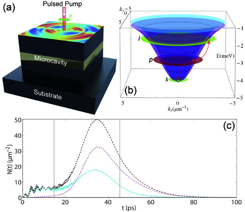
Figure 1: (Color online) (a) Scheme of the microcavity illustrating the pumping geometry. The $X$-polarized (green double arrow) injected polaritons propagate radially outward form the narrow/pulsed pump spot and form circular polarization domains (colormap) [see also Fig.3]. (b) TE (purple surface) and TM (blue surface) lower polariton branches (their energy splitting has been emphasized for clarity). The red disk illustrates the pump ($p$) excitation close to the inflexions of the branches [see Eq.(7)] that are both excited due to the $X$-polarized pump and the smallness of the spot in real space. The green disks mark the signal ($s$) and idler ($i$) states appearing when the OPO is triggered. The red arrows point an example of OPO process occurring along $x$-direction: Two pump polaritons from one branch are scattered toward the signal and idler states of the other branch. (c) Space-integrated densities of the $X$ (solid blue line) $Y$-polarized (dashed pink line) particles and the sum of the two (dashed-dotted black line) revealing the polarization inversion occuring after 25 ps and reaching its maximum at 35 ps. The vertical dashed lines mark the times at which the snapshots of Fig.3 where taken.

Instead of using disorder scattering, it is possible to use a pump spot focused in real space to excite the polariton dispersion on a ringLangbein ; AOSHE ; Sunflower ; NOSHE . The requirement is that the quasi-resonant injection laser, positioned at normal incidence ($\mathbf{k}_{p}=\mathbf{0}$), is blue detuned from the bottom of the polariton branch. The resulting polaritons are then propagating radially outward from the spot with a kinetic energy $E_{k}=\hbar\omega_{p}$, where $\omega_{p}$ is the laser frequency [see Fig.1(a,b)]. This setup allows to obtain a homogeneous and isotropic distribution together with the possibility of investigating nonlinear regimes where disorder is screened.

The asymptotic analytical solution of the Schrödinger equation for a stationary distribution of the polariton spinor field $\bm{\psi}(r,\phi)=(\psi_{+},\psi_{-})^{T}$ can be obtained for the case of a Dirac delta sourceNOSHE at $r=0$:

$${\psi_{+}} = \sqrt{\frac{{2{N_{0}}}}{{\pi{k_{0}}r}}}{e^{-i\phi}}\left[{\cos\phi{e^{i{k_{l}}r}}+i\sin\phi{e^{i{k_{t}}r}}}\right]{e^{-r/{r_{0}}}}$$ (4)

$${\psi_{-}} = \sqrt{\frac{{2{N_{0}}}}{{\pi{k_{0}}r}}}{e^{+i\phi}}\left[{\cos\phi{e^{i{k_{l}}r}}-i\sin\phi{e^{i{k_{t}}r}}}\right]{e^{-r/{r_{0}}}}$$ (5)

Here $N_{0}$ is the population imposed by the source depending on the intensity of the pump. ${r_{0}}=\hbar k_{0}\tau/{m^{*}}$ is a mean decay length where $\tau$, $m^{*}$ and $k_{0}=(k_{l}+k_{t})/2$ are the polaritons lifetime, effective mass and mean excitation wavevector respectively with $k_{l,t}=\sqrt{2m_{l,t}\omega_{P}/\hbar}$ corresponding to the TM ($l$) and TE ($t$) waves respectively. From Eqs.(4,5) we immediately obtain the corresponding distribution of circular polarization degree of the polariton emission $\rho_{c}=(n_{+}-n_{-})/(n_{+}+n_{-})$ where $n_{\pm}=|\psi_{\pm}|^{2}$:

$$\rho_{c}\left(r,\phi\right)=\sin\left[{\left({{k_{l}}-{k_{t}}}\right)r}\right]\sin\left[2\phi\right]$$ (6)

revealing the alternating polarization domains. We see that $\rho_{c}$ is periodic function of both the radial and the angular coordinates. The corresponding radial frequency $\nu_{r}=({k_{l}}-{k_{t}})/2\pi$ is associated with the strength of the TE-TM spitting $\Delta_{lt}$ while the azimuthal one $\nu_{\phi}=\pi$ is imposed by the symmetry of the effective magnetic field $\mathbf{H}_{lt}$. Interestingly, each circular polarization extremum is associated with a phase dislocation while the total density $n_{+}+n_{-}$ remains smooth. This is characteristic of a skyrmion as found in Ref.NOSHE, .

III Polarization inversion

The OSHE is a linear effect which does not involve polariton-polariton scattering. However, taking into account these nonlinear processes can bring qualitative changes to the related polarization textures and spin currents patterns. We have recently shown that in a regime where the interactions are dominant, the polarization currents become strongly focused and the skyrmions turn into half-solitonsNOSHE . This effect is due to the spin-anisotropy of polaritons self-interactions: The polaritons having the same spin projection interact much more efficiently than polaritons with opposite spinsCiuti ; Combescot , the latter process being of the second order. Moreover, the corresponding matrix elements can have opposite signs. This feature is responsible for number of spin dependent nonlinear effects such as polarization multistabilityMultistability , self-induced Larmor precessionSILP , linear polarization build up in polariton condensatesBECPolaritons and the inversion of linear polarization in polariton parametric scatteringRenucci . The latter effect is central for the purposes of the present paper as we will see now.

Due to the their hybrid nature, the shape of the lower polariton branch is strongly non-parabolicMicrocavities , which leads to the appearance of the so-called magic angle close to the inflexion point characterized by the wavenumber $k_{p}$. Two identical polaritons with $\mathbf{k}=\mathbf{k}_{p}$ can scatter to singlet states with $\mathbf{k}_{s}=0$ and $\mathbf{k}_{i}=2\mathbf{k}_{p}$ conserving both the momentum and the energy:

$$E\left({2{\mathbf{k}_{p}}}\right)=2E\left({{\mathbf{k}_{p}}}\right)$$ (7)

Therefore, under quasi-resonant pumping at the magic angle, the system is driven into the so-called optical parametric oscillator regimeOPO (OPO). We note that with increasing pump power, the injected mode becomes more and more blueshifted due to polariton- polariton interactions and therefore the final state selection can be power dependentWhittakerPRB . In polarization resolved OPO experiments under linearly polarized excitation, the final states where found to be cross polarized with respect to the pumpRenucci ; PolInv1D which was theoretically explained using semi-classical spin-dependent kinetic equations containing the terms of spin- anisotropic polariton- polariton scattering SILP ; ShelykhKin ; ReviewSpin . Later on, it was shown that the effect of polarization inversion is universal and can be experimentally observed in other pump geometries, e.g. in two pump horizontal parametric scatteringPolInv . Combined with the pseudospin rotation provided by effective TE-TM field, the effect of parametric polarization inversion can lead to dramatic changes in the pattern of spin currents as we will see in the next section.

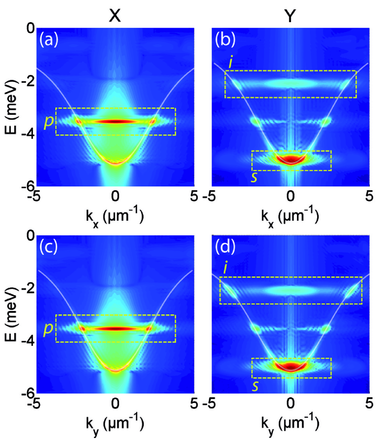
Figure 2: (Color online) Time integrated (over 100 ps) $X$ (a,c) and $Y$ (b,d) dispersions along the $k_{x}$ (a,b) and $k_{y}$ (c,d) directions. The white lines are fits using Eqs.(12) and the dashed yellow frames highlight the signal ($s$), pump ($p$) and idler ($i$) states [see Fig.1(b)].

IV The model

We consider the disorder-free microcavity pumped by a laser spot strongly localized in the real space. Differently from the situation considered in Ref.Langbein, , we take into account nonlinearities provided by spin-anisotropic polariton-polariton interactions and focus on the regime where the system is driven to OPO.

In the absence of the TE-TM splitting, the polaritons eigen modes are degenerated and fully isotropic in the 2D space $E_{l}(k_{r})=E_{t}(k_{r})$. Therefore using the pumping scheme described in Sec.II [Fig.1(a)] while carefully selecting the pump energy $\hbar\omega_{p}$, it should actually be possible to reach the stationary OPO condition over the whole elastic circle (ring OPO) under $cw$ excitation. This would give rise to a trichromatic nonlinear polariton cloud expanding radially from the localized excitation spot. However, when the energy splitting is taken into account, as it should be, the TE and TM modes gain slightly different effective masses $m_{\phi}^{t}$ and $m_{\phi}^{l}$ and on the linear polarization basis, the dispersion branches $E_{X}(\mathbf{k})$ and $E_{Y}(\mathbf{k})$ become anisotropic. This is immediately seen from the basis transformation

$$\left(\begin{array}[]{l}{E_{X}}\left({{k_{r}},{k_{\phi}}}\right)\\ {E_{Y}}\left({{k_{r}},{k_{\phi}}}\right)\end{array}\right)=\left({\begin{array}[]{*{20}{c}}{\cos\left({{k_{\phi}}}\right)}&{\sin\left({{k_{\phi}}}\right)}\\ {-\sin\left({{k_{\phi}}}\right)}&{\cos\left({{k_{\phi}}}\right)}\end{array}}\right)\left(\begin{array}[]{l}{E_{l}}\left({{k_{r}}}\right)\\ {E_{t}}\left({{k_{r}}}\right)\end{array}\right)$$ (8)

It means that exciting the system with a linearly polarized beam, induces a dependence of the OPO condition on azimuthal angle $k_{\phi}$. To overcome this angular anisotropy we propose to use a pulsed excitation providing a sufficient energy broadening to encompass the magic point for any azimuthal directions. We model the quasi-resonant polariton injection with a set of spin-dependent and driven/dissipative equations for the photonic $\phi(\mathbf{r},t)$ and excitonic $\chi(\mathbf{r},t)$ fields coupled via the strong light matter interaction characterized by the Rabi splitting $\Omega_{R}=10$ meV:

$$i\hbar\frac{{\partial{\phi_{\pm}}}}{{\partial t}}= - \frac{{{\hbar^{2}}}}{{2{m_{\phi}}}}\Delta{\phi_{\pm}}+{\Omega_{R}}{\chi_{\pm}}+\beta{\left({\frac{\partial}{{\partial x}}\mp i\frac{\partial}{{\partial y}}}\right)^{2}}{\phi_{\mp}}$$ (9)

$$+ {P_{\pm}}{e^{-i{\omega_{p}}t}}-\frac{{i\hbar}}{{2{\tau_{\phi}}}}{\phi_{\pm}}$$

$$i\hbar\frac{{\partial{\chi_{\pm}}}}{{\partial t}}= - \frac{{{\hbar^{2}}}}{{2{m_{\chi}}}}\Delta{\chi_{\pm}}+{\Omega_{R}}{\phi_{\pm}}$$ (10)

$$+ \left({{\alpha_{1}}{{\left|{{\chi_{\pm}}}\right|}^{2}}+{\alpha_{2}}{{\left|{{\chi_{\mp}}}\right|}^{2}}}\right){\chi_{\pm}}-\frac{{i\hbar}}{{2{\tau_{\chi}}}}\chi_{\pm}$$

Here $\tau_{\chi}=400$ ps and $\tau_{\phi}=20$ ps are the lifetimes of excitons and photons respectively. The functions ${P}_{+}(\mathbf{r},t)={P}_{-}(\mathbf{r},t)$, corresponding to the $X$- linear polarized pump spot, are 2 $\mu$m large and 20 ps long spatio-temporal Gaussians. The energy of the pump $\hbar\omega_{p}$ is blue detuned by an energy $\delta$ (defined below) from the bottom of the lower polariton branch. $m_{\chi}=0.4m_{0}$, $m_{\phi}=5\times 10^{-5}m_{0}$ are the effective masses of the excitons and cavity photons respectively ($m_{0}$ is the electron mass).

The constant $\beta=\hbar^{2}/4(1/m_{\phi}^{l}-1/m_{\phi}^{t})$ defines the magnitude of the photonic TE-TM splitting with $m_{\phi}^{t}=m_{\phi}$ and $m_{\phi}^{l}=0.95m_{\phi}$ being the effective masses of the TE and TM polarized photonic modes. The corresponding terms give rise to the in-plane effective magnetic field $\mathbf{H}_{LT}(\mathbf{k})$. The constants $\alpha_{1}=6\times 10^{-3}$ meV$\cdot\mu$m² and $\alpha_{2}=-0.2\alpha_{1}$ define the strength of the interaction between polaritons of the same and opposite circular polarizations respectively. All the values of the parameters we consider are typical for GaAs based microcavities.

To find the OPO condition we need to know the bare dispersion relations of the linearly polarized modes. We first find the dispersion relations for the TE and TM polariton modes diagonalizing the $2\times 2$ Hamiltonian corresponding to the exciton-photon coupling

$${M_{l,t}}=\left({\begin{array}[]{*{20}{c}}{E_{\phi}^{l,t}\left({{k_{r}}}\right)}&{{\Omega_{R}}}\\ {{\Omega_{R}}}&{E_{\chi}\left({{k_{r}}}\right)}\end{array}}\right)$$ (11)

where $E_{\phi}^{l,t}=\hbar^{2}k_{r}^{2}/2m_{\phi}^{l,t}$ are photonic dispersions for TE and TM polarized modes, and $E_{\chi}=\hbar^{2}k_{r}^{2}/2m_{\chi}$ is the excitonic dispersion, for which we supposed the longitudinal- transverse splitting to be negligibly small. The resulting polariton dispersions are given by the well known expressions

$${E_{l,t}}\left({{k_{r}}}\right)=\frac{E_{\phi}^{l,t}+E_{\chi}}{2}-\frac{1}{2}\sqrt{{{\left({E_{\phi}^{l,t}-E_{\chi}}\right)}^{2}}+4\Omega_{R}^{2}}$$ (12)

which reveal the strong nonparabolicity in the vicinity of the inflexion point. The transformation to the basis of $X$ and $Y$ polarized states can then be done using Eq.(8).

The energy of the angle dependent OPO conditions is found from the solution of Eq.(7). For the previously defined parameters, we obtain that depending on the angle $k_{\phi}$ the magic point lies in the interval of energies ${\Delta E_{OPO}}=\left[{-3.88,-3.78}\right]$ meV and the corresponding interval of wavevectors ${\Delta k_{OPO}}=\left[{1.49,1.58}\right]\mu$m^-1. In the numerical simulations we then impose a detuning $\delta=1.17$ meV. We consider an intermediate pump power slightly above the OPO threshold in order to remain in a regime where the interactions are not dominant and to avoid the onset of the strong spin focusingNOSHE . Finally, we note that Eqs.(9,10) don’t allow for spontaneous scattering by themselves and to trigger the OPO process, we have added to them an additional term corresponding to a weak background gaussian-correlated noise. A weak $Y$ polarized probe at $k=0$ could be used as wellTOPO .

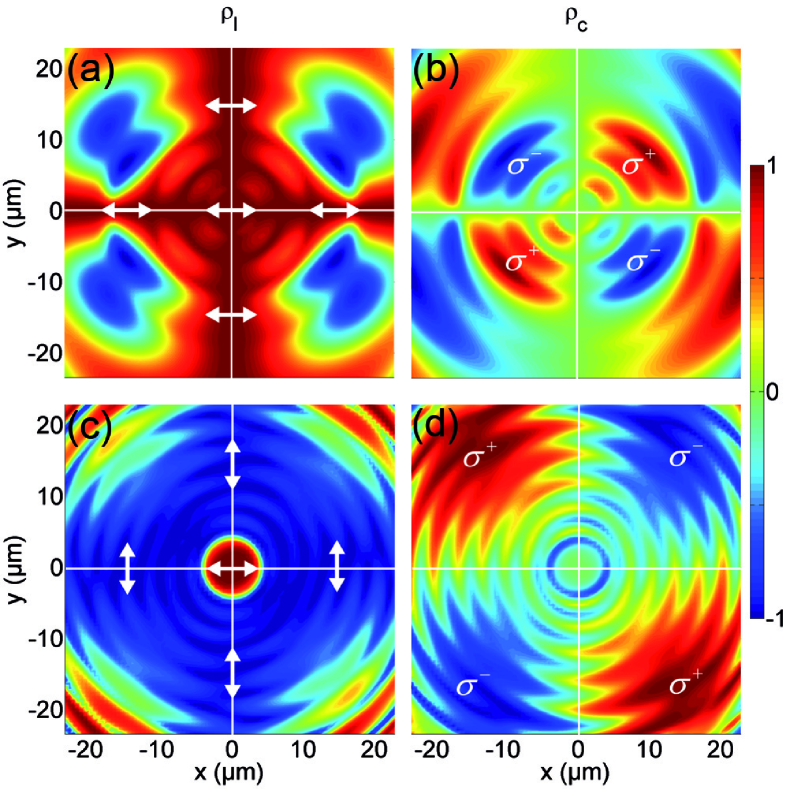
Figure 3: (Color online) Degrees of linear $\rho_{l}$ (a,c) and circular $\rho_{c}$ (b,d) polarization of the photonic polariton components shown before (a,b) ($t=15$ ps) and after (c,d) ($t=45$ ps) the polarization inversion. The double arrows show the polarization directions that are rotated by $\pi/2$ between (a) and (c) in cross directions. In the diagonal directions the circularly polarized domains are inverted between (b) and (d) highlighting the spin current inversion.

V Results and discussion

The results are presented in Figs.1(c), 2 and 3. The panel (c) of Fig.1 shows the space integrated photonic density of the $X$ (solid blue line), $Y$ (solid pink line) polarized polariton and the sum of the two (black line) versus time revealing the $X$-polarized pulsed excitation and the polarization inversion produced by the OPO. Indeed, initially the polariton emission is mainly $X$-polarized until the OPO stimulation becomes strong from about 25 ps, when it starts to be dominated by the $Y$ polarization due to the rotation of the pseudospin of the scattered polaritons.

The Fig.2 shows slices of the $X$ and $Y$ dispersions [panels (a,c) and (b,d) respectively] along the $k_{x}$ and $k_{y}$ direction [panels (a,b) and (c,d)] integrated over 100 ps. These representations capture most of the OPO and inversion features in a single representation. We clearly see the pump ($p$) state in the $X$-component and the signal ($s$) and idler ($i$) states appearing in the $Y$ component. Note that although we pump with $X$-polarized light, the pump state is slightly visible in the $Y$-component as well. This is simply due to the $X$ to $Y$ polarization conversion provided by TE-TM splitting away from the spot prior the inversion [blue regions in Fig.3(a)].

The Fig.3 shows the degrees of linear $\rho_{l}=\Re(\phi_{+}\phi_{-}^{*})/(n_{\phi+}+n_{\phi-})$ [panels (a,c)] and circular $\rho_{c}=(n_{\phi+}-n_{\phi-})/(n_{\phi+}+n_{\phi-})$ [panels (b,d)] polarization of the photonic component (the quantity measured experimentally) at $t=15$ ps and $t=45$ ps respectively (vertical dashed lined in Fig.1(c)). Before the polarization inversion (onset of the OPO) [panels (a,b)] the diagonal polarization domains are those expected for the linear OSHE, while as soon as the OPO is triggered [panels (c,d)], at the edges of the spot the $X$-polarized pump polaritons are instantly converted to the $Y$-polarized polaritons in the signal and idler states. We then have a situation equivalent to the excitation in $Y$ polarization corresponding to $\mathbf{S}_{0}=-S_{x}\mathbf{u}_{x}$. Consequently, as can be seen from Eq.(3) the pseudospin precession is reversed under $\mathbf{S}\rightarrow-\mathbf{S}$ and the circular polarization domains become inverted ($\sigma_{+}\leftrightarrow\sigma_{-}$) which corresponds to an inversion of the spin currents. Importantly, the outgoing nonlinear waves are bichromatic and have two different wavevectors associated to the signal and idler states, which explains the interferences visible in the panel (d). The pump state is emptied due to the pulsed excitation [see Fig.1(c)]. The dominant contribution to the measurable photonic component is the signal state since the $k$-dependent photonic fraction $F_{\phi}(k)$ of polaritons decreases from 0.5 in the signal to less than 0.1 in the idler. It can be easily checked finding the eigenvectors of $M_{l,t}$ and yielding

$${F_{\phi}}=\frac{{4\Omega_{R}^{2}-\Delta{E_{l,t}}\left({\Delta{E_{l,t}}+\sqrt{\Delta E_{l,t}^{2}+4\Omega_{R}^{2}}}\right)}}{{2\Delta E_{l,t}^{2}+8\Omega_{R}^{2}}}$$ (13)

where $\Delta E_{l,t}=E_{\phi}^{l,t}-E_{\chi}$. When the OPO scattering occurs, most of the emission comes from the $Y$-polarized signal state close to $k=0$, which explains why the polarization domains become more extended in real space [compare panels (b) and (d)]. Indeed, the $k$-dependent precession becomes slower [see Eqs.(2,12)] in this state as expected for a reduced value of $\Delta_{lt}(k)$.

We should stress that we worked in a regime where the compression of the polarization domains due to nonlinearities is weak which corresponds to the formation of a skyrmion lattice in terms of Ref.NOSHE, . Therefore, we consider the interval of pump powers intermediate between the linear regime considered in Ref.Langbein, and strongly nonlinear regime considered in Ref.NOSHE, . Interestingly, during the inversion the phase singularity of each skyrmion is transferred from one component to the other. Additionally, one can expect that a further increase of the pump in the OPO regime would lead to the focusing of the inverted spin currents. This would actually compete with the relatively small group velocity in the signal state that makes the polaritons decay before the non-linear effects, that trigger the spin focusing, start to play a strong role.

VI Conclusions

In summary, we have shown that the optical parametric oscillations can be triggered on a whole elastic circle in planar microcavities under pulsed excitation. This regime is associated with the onset of linear polarization inversion leading to the inversion of the spin currents of the optical spin-Hall effect. Together with the effect of nonlinear focusing described earlier in Ref.NOSHE, , we have proposed two mechanisms allowing to control the spin currents in semiconductor microcavities which could be crucial for future spinoptronic applications.

VII Acknowledgments

We acknowledge the support of the FP7 ITN Spin-Optronics (237252) and IRSES ”POLAPHEN” (246912) project. I. A. S. benefited from Rannis ”Center of Excellence in polaritonics” and IRSES ”SPINMET” project.

References

- (1) T. Dieti, D. D. Awschalom, M. Kaminska and H. Ohno, Spintronics, Elsevier (2008).
- (2) I. Shelykh et al., Phys. Rev. B 70, 035320 (2004).
- (3) For a recent review on the topic see: T. C. H. Liew, I. A. Shelykh and G. Malpuech, doi:10.1016/j.physe.2011.04.003.
- (4) A. V. Kavokin, J. J. Baumberg, G. Malpuech, and F. P. Laussy, Microcavities (Oxford University Press, Oxford, 2007).
- (5) E. Wertz, L. Ferrier, D. D. Solnyshkov, R. Johne, D. Sanvitto, A. Lemaître, I. Sagnes, R. Grousson, A. V. Kavokin, P. Senellart, G. Malpuech, and J. Bloch, Spontaneous formation and optical manipulation of extended polariton condensates, Nature Physics 6, 860 (2010).
- (6) C. Adrados, T. C. H. Liew, A. Amo, M. D. Martin, D. Sanvitto, C. Antón, E. Giacobino, A. Kavokin, A. Bramati, and L. Vina, Phys. Rev. B 107, 146402 (2011).
- (7) A. Baas, J.-Ph. Karr, M. Romanelli, A. Bramati, and E. Giacobino, Phys. Rev. B 70, 161307(R) (2004).
- (8) P. G. Savvidis, J. J. Baumberg, R. M. Stevenson, M. S. Skolnick, D. M. Whittaker, and J. S. Roberts, Phys. Rev. Lett. 84, 1547 (2000).
- (9) I. Carusotto, and C. Ciuti, (preprint) arXiv:1205.6500 (2012).
- (10) K. G. Lagoudakis, M. Wouters, M. Richard, A. Baas, I. Carusotto, R. André, Le Si Dang, and B. Deveaud-Plédran, Nature Physic, 4, 706 (2008).
- (11) K. G. Lagoudakis, T. Ostatnický, A. V. Kavokin, Y. G. Rubo, R. André, and B. Deveaud-Plédran, Science 326, 974 (2009).
- (12) A. Amo, S. Pigeon, D. Sanvitto, V. G. Sala, R. Hivet, I. Carusotto, F. Pisanello, G. Leménager, R. Houdré, E Giacobino, C. Ciuti, and A. Bramati, Science 3, 1167 (2011).
- (13) R. Hivet, H. Flayac, D. D. Solnyshkov, D. Tanese, T. Boulier, D. Andreoli, E. Giacobino, J. Bloch, A. Bramati, G. Malpuech, A. Amo, Nat. Phys. 8, 724 728 (2012).
- (14) I. A. Shelykh et al., Semicond. Sci. Technol. 25, 013001 (2010).
- (15) A. Kavokin, G. Malpuech, and M. Glazov, Phys. Rev. Lett. 95, 136601 (2005).
- (16) C. Leyder et al., Nature Phys. 3, 628 (2007).
- (17) A. Amo et al., Phys. Rev. B 80, 165325 (2009).
- (18) M. Maragkou et al., Opt. Lett. 36, 1095 (2011).
- (19) E. Kammann, T. C. H. Liew, H. Ohadi, P. Cilibrizzi, P. Tsotsis, Z. Hatzopoulos, P. G. Savvidis, A. V. Kavokin, and P. G. Lagoudakis, Phys. Rev. Lett. 109, 036404 (2012).
- (20) H. Flayac, D. D. Solnyshkov, I. A. Shelykh, and G. Malpuech, (preprint) arXiv:1207:3533 (2012).
- (21) Y. Kato et al., Science 306, 1910 (2004).
- (22) M. I. Dyakonov and V. I. Perel, Sov. Phys. JETP Lett. 13, 467 (1971).
- (23) S. Murakami, N. Nagaosa, and S.-C. Zhang, Science 301, 1348 (2003).
- (24) I. A. Shelykh, G. Pavlovic, D. D. Solnyshkov, and G. Malpuech, Phys. Rev. Lett. 102, 046407 (2009).
- (25) M. Z. Maialle et al., Phys. Rev. B 47, 15776 (1993).
- (26) G. Panzarini et al., Phys. Rev. B 59, 5082 (1999).
- (27) W. Langbein et al., Phys. Rev. B 75, 075323 (2007).
- (28) G. Christmann, G. Tosi, N. G. Berloff, P. Tsotsis, P. S. Eldridge, Z. Hatzopoulos, P. G. Savvidis, and J. J. Baumberg, Phys. Rev. B 85, 235303 (2012).
- (29) C. Ciuti et al., Phys. Rev. B 58, 7926 (1998).
- (30) M. Combescot and O. Betbeder-Matibet, Phys. Rev. B 74, 125316 (2006).
- (31) N. A. Gippius, I. A. Shelykh, D. D. Solnyshkov, S. S. Gavrilov, Yuri G. Rubo, A. V. Kavokin, S. G. Tikhodeev, and G. Malpuech, Phys. Rev. Lett. 98, 236401 (2007).
- (32) D. N. Krizhanovskii, D. Sanvitto, I. A. Shelykh, M. M. Glazov, G. Malpuech, D. D. Solnyshkov, A. Kavokin, S. Ceccarelli, M. S. Skolnick, and J. S. Roberts, Phys. Rev. B 73, 073303 (2006).
- (33) J. Kasprzak, M. Richard, S. Kundermann, A. Baas, P. Jeambrun, J. M. J. Keeling, F. M. Marchetti, M. H. Szymaska, R. André, J. L. Staehli, V. Savona, P. B. Littlewood, B. Deveaud, and Le Si Dang, Nature 443, 409 (2006).
- (34) P. Renucci et al., Phys. Rev. B 72, 075317 (2005).
- (35) D. M. Whittaker, Phys. Rev. B 71, 115301 (2005).
- (36) G. Dasbach et al., Phys. Rev. B 71, 161308(R) (2005).
- (37) C. Leyder et al., Phys. Rev. Lett. 99, 196402 (2007).
- (38) I. A. Shelykh, M. M. Glazov, D. D. Solnyshkov, N. G. Galkin, A. V. Kavokin, and G. Malpuech, Phys. Stat. Sol. (c) 2, 768 (2005).
- (39) D. Sanvitto, F. M. Marchetti, M. H. Szymanska, G. Tosi, M. Baudisch, F. P. Laussy, D. N. Krizhanovskii, M. S. Skolnick, L. Marrucci, A. Lemaître, J. Bloch, C. Tejedor, and L. Vina, Nature Physics 6, 527 (2010).