Gap-modulated doping effects on indirect exchange interaction between magnetic impurities in graphene

Abstract

A dilute distribution of magnetic impurities is assumed to be present in doped graphene. We calculate the interaction energy between two magnetic impurities which are coupled via the indirect-exchange or Ruderman-Kittel-Kasuva-Yosida (RKKY) interaction by the doped conduction electrons. The current model is a half-filled $AB$-lattice structure. Our calculations are based on the retarded lattice Green’s function formalism in momentum-energy space which is employed in linear response theory to determine the magnetic susceptibility in coordinate space. Analytic results are obtained for gapped graphene when the magnetic impurities are placed on the $A$ and $B$ sublattice sites of the structure. This interaction, which is important in determining spin ordering, has been found to be significantly different for $AA$ and $BB$ exchange energies in doped graphene due to the existence of an energy gap, and is attributed to a consequence of the local fields not being equal on the $A$ and $B$ sublattices. For doped graphene, the oscillations of all three RKKY interactions from ferromagnetic to antiferromagnetic with increasing Fermi energy is significantly modified by the energy gap both in magnitude and phase. Additionally, the $AB$ exchange energy may be modified by the presence of a gap for undoped graphene but not for doped graphene due to the dominance of doped conduction electrons.

I Introduction

Recently, there has been some attention given to the effects arising from the Ruderman-Kittel-Kasuva-Yosida (RKKY) RKKY1 ; RKKY2 ; RKKY3 or indirect-exchange interaction between spins via the host conduction electrons of monolayer free standing graphene, a two-dimensional honeycomb network of carbon atoms RKKYG1 ; RKKYG2 ; RKKYG3 ; RKKYG4 ; RKKYG5 ; RKKYG6 ; RKKYG7 ; RKKYG8 . Such local moments may arise near extended defects. Interest in the RKKY interaction is due partially to the fact that it determines spin ordering. The indirect exchange interaction between local magnetic moments is generally determined by electron excitations near the Fermi level. However, although the RKKY interaction has been considered in intrinsic graphene by several authors, little attention has been given to its role when a gap $2E_{g}$ is opened at the two inequivalent $K$ and $K^{\prime}$ points in momentum space between the valence and conduction bands pavlo ; 7 ; 8 ; kibis ; OR1 ; OR2 . This effective band gap may be generated by spin-orbit interaction RKKYG7 . It may also arise when monolayer graphene is placed on a substrate such as ceramic silicon carbide 7 or graphite 8 or dynamically when it is irradiated by circularly polarized light kibis ; OR1 ; OR2 . Depending on the nature of the substrate on which graphene is placed or the intensity and amplitude of the light, the gap may be a few meV or as large as an eV. In general, the energy gap is attributed to a breakdown in symmetry between the sublattices caused by external perturbing fields from the substrate or photons coupled to the $A$ and $B$ atoms. Furthermore, there still exists a small band gap $2E_{\rm so}\sim 10^{-3}$ meV due to spin-orbit coupling 9 ; 9b even in the absence of a substrate or an external laser field. Despite the formation of an energy band gap, corresponding to a metal-insulator transition, for the half-filled bipartite lattice, the interaction between atoms on the same lattice has still been suggested to be ferromagnetic and antiferromagnetic between atoms on different sublattices in undoped graphene RKKYG6 , even though the energy dispersion is no longer linear and isotropic as it is for gapless Dirac electrons. For undoped graphene, we show that the existence of an energy gap can significantly modify the magnitude of the magnetic interaction between impurities on the sublattices. More interestingly, for doped graphene, we demonstrate that the energy gap can drastically affect the nature of such a magnetic interaction.

In Ref. [RKKYG7, ], with a small gap at the Fermi level due to spin-orbit interaction, the graphene layer was assumed to be undoped. The present paper explores quantitatively the role played by massive relativistic Dirac particles in both doped and undoped graphene on the RKKY indirect-exchange energy. In other words, how the magnetic effects depend on the chirality of the electron states for doped graphene with an energy gap. Analytic results are obtained for gapped graphene when both impurities are located on sites belonging to the $A$ sublattice, both on the $B$ sublattice and when one impurity is on an $A$ while the other is on a $B$ sublattice site. We demonstrate numerically the large asymmetry between the $AA$ and $BB$-exchange-interaction energy for gapped graphene. Our closed-form analytic results make it convenient for our predictions to be compared with experimental data once they become available.

The remainder of this paper is organized as follows. In Sec. II, we obtain the retarded Green’s function matrix elements on the $A$ and $B$ sublattices for gapped graphene. In Sec. III, we use linear response theory to calculate the magnetic susceptibility by making use of our derived results for the Green’s functions on the bipartite sublattices. The interaction energy of two spins at lattice sites $r_{\mu}$ and $r_{\nu}^{\prime}$, where $\mu,\,\nu=A,\,B$, is then deduced for both undoped and doped gapped graphene. We conclude our paper in Sec. IV with some remarks.

II Green-Function Formalism for Graphene

The Hamiltonian for monolayer gaped graphene in the absence of impurities has the form:

$${\cal H}(\mathbf{k})=\left[{\begin{matrix}E_{g}&-\gamma_{0}h_{0}^{\star}(\mathbf{k})\\ -\gamma_{0}h_{0}(\mathbf{k})&-E_{g}\end{matrix}}\right]\ ,$$ (1)

where

$$h_{0}(\mathbf{k})=\exp\left({ik_{y}a}\right)+\exp\left({-\frac{i\sqrt{3}ak_{x}}{2}-\frac{iak_{y}}{2}}\right)+\exp\left({\frac{i\sqrt{3}ak_{x}}{2}-\frac{iak_{y}}{2}}\right)$$ (2)

with the carbon-carbon distance $a=1.14$ Å, $\gamma_{0}=-3.0\,\texttt{eV}$ and $\mathbf{k}=(k_{x},k_{y})$. Here, $2E_{g}$ is the energy gap generated by some means, possibly by a substrate or circularly polarized light, as discussed in the Introduction. The retarded Green’s function matrix in wave vector-energy ($\mathbf{k},E$) space is given by

$$G\left({\mathbf{k},E}\right) = \left[{E-{\cal H}(\mathbf{k})+i0^{+}}\right]^{-1}$$ (3)

$$= \frac{1}{E^{2}-E_{g}^{2}-\gamma_{0}^{2}\,h_{0}(\mathbf{k})h_{0}^{\star}(\mathbf{k})}\left[{\begin{matrix}E_{g}+E&\gamma_{0}h_{0}^{\star}(\mathbf{k})\\ \gamma_{0}h_{0}(\mathbf{k})&-E_{g}+E\end{matrix}}\right]\equiv\left[{\begin{matrix}G_{AA}&G^{\star}_{AB}\\ G_{AB}&G_{BB}\end{matrix}}\right]$$

with

$$G_{AA}\left({\mathbf{k},E}\right) = \frac{1}{E^{2}-E^{2}_{\mathbf{k}}}\,(E_{g}+E)\ ,$$

$$G_{BB}\left({\mathbf{k},E}\right) = \frac{1}{E^{2}-E^{2}_{\mathbf{k}}}\,(-E_{g}+E)\ ,$$

$$G_{AB}\left({\mathbf{k},E}\right) = G^{\star}_{BA}\left({\mathbf{k},E}\right)=\frac{1}{E^{2}-E^{2}_{\mathbf{k}}}\,\gamma_{0}h_{0}(\mathbf{k})\ ,$$

where we introduced the energy dispersion equation $E^{2}_{\mathbf{k}}=\gamma_{0}^{2}\,h_{0}(\mathbf{k})\,h_{0}^{\star}(\mathbf{k})+E^{2}_{g}$.

We may now transform the Green’s function to the real space representation with use of

$$G(\mathbf{r},\mathbf{r}^{\prime},E) = \int\limits_{\texttt{1${}^{\rm st}$\,BZ}}d^{2}\mathbf{k}\ G(\mathbf{k},E)\exp\left[{i\mathbf{k}\cdot\left({\mathbf{r}-\mathbf{r}^{\prime}}\right)}\right]$$ (5)

$$= \frac{S}{4\pi^{2}}\sum\limits_{i=1}^{6}\int\limits dk_{x}dk_{y}\,G(\mathbf{K}_{i}+\mathbf{k},E)\exp\left[{i\left({\mathbf{K}_{i}+\mathbf{k}}\right)\cdot\left({\mathbf{r}-\mathbf{r}^{\prime}}\right)}\right]\ ,$$

where the summation is carried out over the six corners of the Brillouin zone (BZ), so that we may make the approximation $E^{2}_{\mathbf{K}_{i}+\mathbf{k}}=\left({\gamma k}\right)^{2}+E^{2}_{g}$ with $\gamma=3a\gamma_{0}/2$. In that approximation, we also have $\gamma_{0}h_{0}=\gamma k$. Additionally, in our notation, the area of the unit cell is $S=3\sqrt{3}a^{2}/2$.

Using cylindrical coordinates, the matrix elements of the retarded Green’s function may be explicitly written as

$$G_{AA}(\textbf{r}_{A},\textbf{r}^{\prime}_{A};E) = {\frac{2S}{(2\pi)^{2}}}\,\cos[\textbf{K}_{1}\cdot(\textbf{r}_{A}-\textbf{r}^{\prime}_{A})]\int\limits_{0}^{2\pi}d\theta\int\limits_{0}^{k_{c}}dk\ k{G_{AA}(k,E)}\,e^{i\textbf{k}\cdot(\textbf{r}_{A}-\textbf{r}^{\prime}_{A})}\ ,$$

$$G_{BB}(\textbf{r}_{B},\textbf{r}^{\prime}_{B};E) = {\frac{2S}{(2\pi)^{2}}}\,\cos[\textbf{K}_{1}\cdot(\textbf{r}_{B}-\textbf{r}^{\prime}_{B})]\int\limits_{0}^{2\pi}d\theta\int\limits_{0}^{k_{c}}dk\ k{G_{BB}(k,E)}\,e^{i\textbf{k}\cdot(\textbf{r}_{B}-\textbf{r}^{\prime}_{B})}\ ,$$

$$G_{AB}(\textbf{r}_{A},\textbf{r}^{\prime}_{B};E) = G^{\star}_{BA}(\textbf{r}^{\prime}_{B},\textbf{r}_{A};E)$$ (6)

$$= {\frac{S}{(2\pi)^{2}}}\{e^{i\textbf{K}_{1}(\textbf{r}_{A}-\textbf{r}^{\prime}_{B})}\int\limits_{0}^{2\pi}d\theta\int\limits_{0}^{k_{c}}dk\ k(-i\sin\theta-\cos\theta){G_{AB}(k,E)}\,e^{i\textbf{k}\cdot(\textbf{r}_{A}-\textbf{r}^{\prime}_{B})}$$

$$+ e^{-i\textbf{K}_{1}(\textbf{r}_{A}-\textbf{r}^{\prime}_{B})}\int\limits_{0}^{2\pi}d\theta\int\limits_{0}^{k_{c}}dk\ k(-i\sin\theta+\cos\theta){G_{AB}(k,E)}\,e^{i\textbf{k}\cdot(\textbf{r}_{A}-\textbf{r}^{\prime}_{B})}\}\ ,$$

where $k_{c}$ is a cut-off wave vector whose existence is due to the fact that the energy band structure used in the calculation is only valid for a limited range of the first BZ near the $K$ points. However, it is also allowed in such an approximation to take the limit $k_{c}\to\infty$ from a mathematical point of view. In the above expression, we have $\textbf{K}_{1}=(4\pi/3\sqrt{3}a,0)$.

We now make use of the following identity involving the series of the first kind of Bessel function $J_{n}(x)$

$$e^{i\textbf{k}\cdot(\textbf{r}_{\mu}-\textbf{r}^{\prime}_{\nu})}=J_{0}(k|\textbf{r}_{\mu}-\textbf{r}^{\prime}_{\nu}|)+2\,{\sum\limits_{n=1}^{\infty}}\,i^{n}J_{n}(k|\textbf{r}_{\mu}-\textbf{r}^{\prime}_{\nu}|)\cos(n\varphi_{r_{\mu},r^{\prime}_{\nu}})\ ,$$ (7)

where $(\mu,\nu)\equiv(A,B)$ and $\varphi_{r_{\mu},r^{\prime}_{\nu}}$ is the angle between k and $\textbf{r}_{\mu}-\textbf{r}^{\prime}_{\nu}$. We may calculate the above integrals and simplify the real-space Green’s function matrix elements as

$$G_{AA}(\textbf{r}_{A},\textbf{r}_{A}^{\prime};E) = \cos[\textbf{K}_{1}\cdot(\textbf{r}_{A}-\textbf{r}^{\prime}_{A})]\,F_{1}(|\textbf{r}_{A}-\textbf{r}^{\prime}_{A}|,E)\ ,$$

$$G_{BB}(\textbf{r}_{B},\textbf{r}_{B}^{\prime};E) = \cos[\textbf{K}_{1}\cdot(\textbf{r}_{B}-\textbf{r}^{\prime}_{B})]\,F_{2}(|\textbf{r}_{B}-\textbf{r}^{\prime}_{B}|,E)\ ,$$

$$G_{AB}(\textbf{r}_{A},\textbf{r}_{B}^{\prime};E) = G^{\star}_{BA}(\textbf{r}_{B}^{\prime},\textbf{r}_{A};E)=\sin[\textbf{K}_{1}\cdot(\textbf{r}_{A}-\textbf{r}^{\prime}_{B})+\alpha_{r_{A},r^{\prime}_{B}}]\,F_{3}(|\textbf{r}_{A}-\textbf{r}^{\prime}_{B}|,E)\ .$$ (8)

In this notation, $\cos(\varphi_{r_{\mu},r^{\prime}_{\nu}})=\cos(\theta-\alpha_{r_{\mu},r^{\prime}_{\nu}})$, where $\theta$ is the angle which k makes with the $x$-axis, and $\alpha_{r_{\mu},r^{\prime}_{\nu}}$ is the angle between $\textbf{r}_{\mu}-\textbf{r}^{\prime}_{\nu}$ and the $x$-axis. Three position-dependent complex functions $F_{j}(|\textbf{r}_{\mu}-\textbf{r}^{\prime}_{\nu}|,E)$ for $j=1,\,2,\,3$ are defined as follows:

$$F_{1}(|\textbf{r}_{\mu}-\textbf{r}^{\prime}_{\nu}|,E) = \frac{S}{\pi}{\int\limits_{0}^{\infty}}dk\ kJ_{0}(k|\textbf{r}_{\mu}-\textbf{r}^{\prime}_{\nu}|)\,\frac{E_{g}+E}{E^{2}-(\gamma k)^{2}-E^{2}_{g}}$$

$$= -\frac{S}{\pi\gamma^{2}}\left[{(E+E_{g})K_{0}\left({\frac{i\sqrt{E^{2}-E_{g}^{2}}}{\gamma}|\textbf{r}_{\mu}-\textbf{r}^{\prime}_{\nu}|}\right)}\right]\ ,$$

$$F_{2}(|\textbf{r}_{\mu}-\textbf{r}^{\prime}_{\nu}|,E) = \frac{S}{\pi}{\int\limits_{0}^{\infty}}dk\ kJ_{0}(k|\textbf{r}_{\mu}-\textbf{r}^{\prime}_{\nu}|)\,\frac{-E_{g}+E}{E^{2}-(\gamma k)^{2}-E^{2}_{g}}$$

$$= -\frac{S}{\pi\gamma^{2}}\left[{(E-E_{g})K_{0}\left({\frac{i\sqrt{E^{2}-E_{g}^{2}}}{\gamma}|\textbf{r}_{\mu}-\textbf{r}^{\prime}_{\nu}|}\right)}\right]\ ,$$

$$F_{3}(|\textbf{r}_{\mu}-\textbf{r}^{\prime}_{\nu}|,E) = \frac{S}{\pi}{\int\limits_{0}^{\infty}}dk\ kJ_{1}(k|\textbf{r}_{\mu}-\textbf{r}^{\prime}_{\nu}|)\,\frac{\gamma k}{E^{2}-(\gamma k)^{2}-E^{2}_{g}}$$ (9)

$$= -\frac{S}{\pi\gamma^{2}}\left[{i\sqrt{E^{2}-E_{g}^{2}}K_{1}\left({\frac{i\sqrt{E^{2}-E_{g}^{2}}}{\gamma}|\textbf{r}_{\mu}-\textbf{r}^{\prime}_{\nu}|}\right)}\right]\ ,$$

where $K_{m}(x)$ for integer $m$ is the modified Bessel function. In addition, we have used the formula for the $m^{\texttt{th}}$ order Hankel transform

$$\int\limits_{0}^{\infty}\ xdx\ \frac{x^{m}}{x^{2}+\alpha^{2}}\,J_{m}(xE)=\alpha^{m}K_{m}(\alpha E)\ ,$$ (10)

where $\alpha$ is an arbitrary constant.

III Indirect-Exchange Interaction Energy

Let us now assume that we have two magnetic impurities with spins $\mathbf{S}_{1}$ and $\mathbf{S}_{2}$) located at $\mathbf{r}_{\mu}$ and $\mathbf{r^{\prime}}_{\nu}$, respectively. According to linear response theory, the energy needed to exchange (mediated by the Dirac electrons) their positions may be written in the matrix form

$${\cal V}_{\mu\nu}(|\textbf{r}_{\mu}-\textbf{r}^{\prime}_{\nu}|)={\cal J}_{\mu\nu}(|\textbf{r}_{\mu}-\textbf{r}^{\prime}_{\nu}|)\,\mathbf{S}_{1}\cdot\mathbf{S}_{2}\ ,$$ (11)

where the exchange-integral matrix is proportional to the matrix of spin-independent susceptibility

$${\cal J}_{\mu\nu}(|\textbf{r}_{\mu}-\textbf{r}^{\prime}_{\nu}|)=\frac{4\lambda^{2}}{\hbar^{2}}\,\chi_{\mu\nu}(|\textbf{r}_{\mu}-\textbf{r}^{\prime}_{\nu}|)\ .$$ (12)

Here, $\lambda$ is the contact interaction between the magnetic impurities and the Dirac electrons. The magnetic susceptibility may be expressed in terms of the Green’s functions in the standard RKKY form RKKY1 ; RKKY2 ; RKKY3 .

III.1 Undoped Graphene with a Gap

For undoped graphene, we take the Fermi energy $E_{F}=0$. For this case, we obtain the matrix of spin-independent susceptibility

$$\chi_{\mu\nu}(|\textbf{r}_{\mu}-\textbf{r}^{\prime}_{\nu}|)=-\frac{2}{\pi}\int\limits_{-\infty}^{-E_{g}}dE\ \texttt{Im}\left[{G(\textbf{r}_{\mu},\textbf{r}_{\nu}^{\prime};E)\,G(\textbf{r}_{\nu}^{\prime},\textbf{r}_{\mu};E)}\right]\ .$$ (13)

Making use of the expressions for the Green’s functions from the preceding section, it is a simple matter to obtain the following matrix elements:

$$\chi_{AA}(|\textbf{r}_{A}-\textbf{r}^{\prime}_{A}|) = -\frac{1}{\pi}\left({1+\cos[2\textbf{K}_{1}\cdot(\textbf{r}_{A}-\textbf{r}^{\prime}_{A})]}\right)\,\texttt{Im}\int\limits_{-\infty}^{-E_{g}}dE\left[{F_{1}(|\textbf{r}_{A}-\textbf{r}^{\prime}_{A}|,E)}\right]^{2}\ ,$$

$$\chi_{BB}(|\textbf{r}_{B}-\textbf{r}^{\prime}_{B}|) = -\frac{1}{\pi}\left({1+\cos[2\textbf{K}_{1}\cdot(\textbf{r}_{B}-\textbf{r}^{\prime}_{B})]}\right)\,\texttt{Im}\int\limits_{-\infty}^{-E_{g}}dE\left[{F_{2}(|\textbf{r}_{B}-\textbf{r}^{\prime}_{B}|,E)}\right]^{2}\ ,$$

$$\chi_{AB}(|\textbf{r}_{A}-\textbf{r}^{\prime}_{B}|) = -\frac{1}{\pi}\left({\cos[2\textbf{K}_{1}\cdot(\textbf{r}_{A}-\textbf{r}^{\prime}_{B})+2\alpha_{r_{A},r^{\prime}_{B}}]-1}\right)$$ (14)

$$\times \texttt{Im}\int\limits_{-\infty}^{-E_{g}}dE\left[{F_{3}(|\textbf{r}_{A}-\textbf{r}^{\prime}_{B}|,E)}\right]^{2}\ .$$

We first consider the case when both impurities are located on $A$ atomic sites. That is, we need to calculate

$${\cal P}_{1}(E_{g},R_{AA})\equiv\texttt{Im}\int\limits_{-\infty}^{-E_{g}}dE\left[{F_{1}(|\textbf{r}_{A}-\textbf{r}^{\prime}_{A}|,E)}\right]^{2}$$ (15)

$$= \frac{S^{2}}{2\gamma^{4}}\int\limits_{-\infty}^{-E_{g}}dE\ \left({E+E_{g}}\right)^{2}J_{0}\left({\frac{-\sqrt{E^{2}-E_{g}^{2}}}{\gamma}\,|\textbf{r}_{A}-\textbf{r}^{\prime}_{A}|}\right)N_{0}\left({\frac{-\sqrt{E^{2}-E_{g}^{2}}}{\gamma}\,|\textbf{r}_{A}-\textbf{r}^{\prime}_{A}|}\right)$$

$$= \frac{2}{3\gamma_{0}}\int\limits_{-\infty}^{-E_{g}}dE\ \left({E+E_{g}}\right)^{2}J_{0}\left({-\frac{2}{3}\sqrt{E^{2}-E_{g}^{2}}\,R_{AA}}\right)N_{0}\left({-\frac{2}{3}\sqrt{E^{2}-E_{g}^{2}}\,R_{AA}}\right)\ ,$$

where $N_{0}(x)$ is the Neumann function. For convenience, in the last expression, we measure energy in units of $\gamma_{0}$ and distance in units of $R_{AA}=|\textbf{r}_{A}-\textbf{r}^{\prime}_{A}|/a$. In the gapless case, $E_{g}=0$, we are able to calculate the integral analytically, obtaining

$${\cal P}^{0}_{1}(R_{AA})\equiv{\cal P}_{1}(0,R_{AA})=\texttt{Im}\int\limits_{-\infty}^{0}dE\ \left[{F_{1}(|\textbf{r}_{A}-\textbf{r}^{\prime}_{A}|,E)}\right]^{2}$$ (16)

$$= \frac{9}{4\gamma_{0}R^{3}_{AA}}\int\limits_{0}^{\infty}dx\,x^{2}\,J_{0}\left({x}\right)N_{0}\left({x}\right)=\frac{9}{64\gamma_{0}R^{3}_{AA}}\ .$$

The last integral may be evaluated through

$$\lim_{x_{0}\rightarrow 0}\int\limits_{0}^{\infty}dx\,x^{2}\exp(-x_{0}x)\,J_{0}\left({x}\right)N_{0}\left({x}\right)$$ (17)

$$= \lim_{x_{0}\to 0}\frac{4\left({4+3x^{2}_{0}}\right){\cal E}(-x_{0}^{2}/4)-2\left({8+6x_{0}^{2}+x_{0}^{4}}\right){\cal K}(-x_{0}^{2}/4)}{\pi x_{0}^{2}\left({4+x_{0}^{2}}\right)^{2}}=\frac{1}{16}\ ,$$

where ${\cal K}(x)$, ${\cal E}(x)$ are the complete elliptic integrals of the first and second kind, respectively.

In a similar fashion, we have for the $AB$ exchange interaction

$${\cal P}_{3}(E_{g},R_{AB}) = \texttt{Im}\int\limits_{-\infty}^{-E_{g}}dE\left[{F_{3}(|\textbf{r}_{A}-\textbf{r}^{\prime}_{B}|,E)}\right]^{2}=-\frac{2}{3\gamma_{0}}\int\limits_{-\infty}^{-E_{g}}dE\,\left(\sqrt{E^{2}-E_{g}^{2}}\right)^{2}$$ (18)

$$\times J_{1}\left({-\frac{2}{3}\sqrt{E^{2}-E_{g}^{2}}R_{AB}}\right)N_{1}\left({-\frac{2}{3}\sqrt{E^{2}-E_{g}^{2}}R_{AB}}\right)\ ,$$

where $N_{1}(x)$ is also the Neumann function. For $E_{g}=0$, the integral may be evaluated analytically, yielding

$$\lim_{x_{0}\to 0}\int\limits_{0}^{\infty}dx\ x^{2}\exp(-x_{0}x)\,J_{1}\left({x}\right)N_{1}\left({x}\right)$$ (19)

$$= \lim_{x_{0}\rightarrow 0}\frac{-4\left({-4+x^{2}_{0}}\right){\cal E}(-x_{0}^{2}/4)-4\left({4+x_{0}^{2}}\right){\cal K}(-x_{0}^{2}/4)}{\pi x_{0}^{2}\left({4+x_{0}^{2}}\right)^{2}}=-\frac{3}{16}\ ,$$

so that we have

$${\cal P}^{0}_{3}(R_{AB})\equiv{\cal P}_{3}(0,R_{AB})=\texttt{Im}\int\limits_{-\infty}^{0}dE\left[{F_{3}(|\textbf{r}_{A}-\textbf{r}^{\prime}_{B}|,E)}\right]^{2}=-\frac{27}{64\gamma_{0}R^{3}_{AB}}\ .$$ (20)

The effects of doping on the indirect-exchange interaction for a graphene layer without a gap have been studied in detail. In this case, a sign change of the indirect-exchange interaction was discovered when the doping concentration was varied. There is a switching from inverse cubic to inverse square power law for the spatial dependence. RKKYG5 However, the doping effect for a graphene layer with a gap remains largely unexplored. To demonstrate the doping effect for gaped graphene, we write ${\cal P}_{j}(E_{g},R_{\mu\nu})={\cal P}^{0}_{j}(R_{\mu\nu})+\Delta{\cal P}_{j}(E_{g},R_{\mu\nu})$ with $\mu,\,\nu=A,\,B$ and $j=1,\,2,\,3$.

In Fig. 1, we present our calculated results for ${\cal P}_{j}(E_{g},R_{\mu\nu})$ (left panel) and $\Delta{\cal P}_{j}(E_{g},R_{\mu\nu})$ (right panel) in an undoped graphene layer as functions $E_{g}$ with $R_{AA}=R_{BB}=R_{AB}=0.5$. From the left panel of this figure, we find that the positive exchange interactions ${\cal P}_{1}$ and ${\cal P}_{2}$ between two intra-sublattice impurities (intra-SIs) decrease with $E_{g}$ while the negative exchange interaction ${\cal P}_{3}$ between two inter-sublattice impurities (inter-SIs) increases with $E_{g}$ at the same time. We further observe that the degenerate ${\cal P}_{1}$ and ${\cal P}_{2}$ at $E_{g}=0$, due to the presence of symmetry with respect to two sublattices, is now lifted for $E_{g}>0$. Compared with the results when $E_{g}=0$. We see from the right panel of this figure that the gap-induced changes $\Delta{\cal P}_{1}$ and $\Delta{\cal P}_{2}$ become more and more negative with increasing $E_{g}$. Additionally, the decrease of $\Delta{\cal P}_{1}$ is more rapid than for $\Delta{\cal P}_{2}$. This behavior reflects a modulation in the exchange interaction by an energy gap in graphene. Also, it suggests a possible gap-induced ferromagnetic-to-antiferromagnetic phase transition due to the intra-SI exchange interaction. In contrast, a distinctly opposite behavior is found in the inter-SI exchange interaction $\Delta{\cal P}_{3}$.

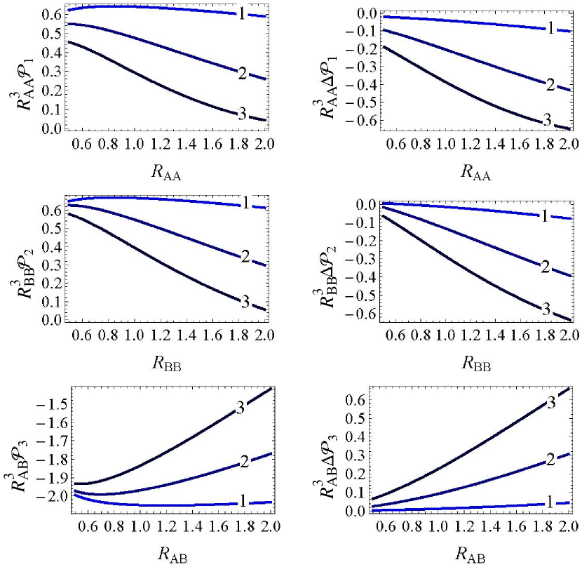
Figure 2: (Color online) Exchange interaction energies $R_{AA}^{3}{\cal P}_{1}$ (top panel), $R_{BB}^{3}{\cal P}_{2}$ (middle panel) and $R_{AB}^{3}{\cal P}_{3}$ (bottom panel) on the left column, as well as the changes of them $R_{AA}^{3}\Delta{\cal P}_{1}$ (top panel), $R_{BB}^{3}\Delta{\cal P}_{2}$ (middle panel) and $R_{AB}^{3}\Delta{\cal P}_{3}$ (bottom panel) on the right column, in undoped graphene as functions of the distance between two magnetic impurities. Curves $1,\,2,\,3$ correspond to gap energy parameter $E_{g}=0.1,\ 0.3,\ 0.5$, respectively. Here, we measure energy in units of $\gamma_{0}$ and distance in units of $R_{\mu\nu}=|\textbf{r}_{\mu}-\textbf{r}^{\prime}_{\nu}|/a$ for $\mu,\,\nu=A,\,B$.

We display in Fig. 2 the calculated results for $R^{3}_{\mu\nu}{\cal P}_{j}(E_{g},R_{\mu\nu})$ (left column) and $R^{3}_{\mu\nu}\Delta{\cal P}_{j}(E_{g},R_{\mu\nu})$ (right column) as functions of the distance $R_{\mu\nu}$ between two magnetic impurities for various values of $E_{g}$ in undoped graphene. From the left column of this figure, we observe clear deviations of the exchange interactions ${\cal P}_{1}$, ${\cal P}_{2}$ and ${\cal P}_{3}$ from $1/R^{3}_{\mu\nu}$ dependence (at $E_{g}=0$) with increasing $E_{g}$ (from curve-1 to curve-3). These results also indicate a possible gap-induced phase transition which may be driven by either the intra-SI or the inter-SI exchange interaction at a relatively large distance between two magnetic impurities in a graphene layer. Additionally, we find from the right column of this figure that changes in $\Delta{\cal P}_{1}$ and $\Delta{\cal P}_{2}$ in the intra-SI exchange interactions drop more rapidly as a function of $R_{\mu\mu}$ when $E_{g}$ is increased. Again, a completely opposite behavior is observed in this case for $\Delta{\cal P}_{3}$ which is associated with the inter-SI exchange interaction.

III.2 Doped Graphene with a Gap

We now turn to the case of doped graphene which has a finite Fermi energy $E_{F}>0$. It is convenient to introduce a dimensionless f the Fermi energy as $X_{F}\equiv\frac{2}{3}E_{F}R_{AA}/\gamma_{0}$. The Fermi energy makes the integration limits in Eqs. (16) and (20) raised to include the part $\int\limits_{E_{g}}^{E_{g}+E_{F}}dE$. In the case when $E_{g}=0$ those integrals assume the analytical forms:

$${\cal P}^{0}_{1}\left({R_{AA}}\right)=\frac{9}{4\gamma_{0}R^{3}_{AA}}\left[{\frac{1}{16}+\frac{{\cal G}_{2,4}^{2,1}\left(X_{F}^{2}\bigg{|}{\begin{array}[]{c}1,2\\ \frac{3}{2},\frac{3}{2},0,\frac{3}{2}\\ \end{array}}\right)}{2\sqrt{\pi}}}\right]\ ,$$ (23)

$${\cal P}^{0}_{3}\left({R_{AB}}\right)=\frac{9}{4\gamma_{0}R^{3}_{AB}}\left[{-\frac{3}{16}-\frac{{\cal G}_{2,4}^{2,1}\left(X_{F}^{2}\bigg{|}{\begin{array}[]{c}1,2\\ \frac{3}{2},\frac{5}{2},0,\frac{1}{2}\\ \end{array}}\right)}{2\sqrt{\pi}}}\right]\ .$$ (26)

Here, ${\cal G}^{m,n}_{p,q}$ is the Meijer’s $G$-function. It has oscillating behavior  thus switching the nature of ${\cal J}_{AA}$ and ${\cal J}_{AB}$ between ferromagnetic and antiferromagnetic. In the long distance limit $R_{AA}\approx R_{AB}\approx R_{BB}$, we can use the mean field approximation as in the work of Sherafati and Satpathy RKKYG3 .

In Fig. 3, we present our calculated results for ${\cal P}_{j}(E_{g},R_{\mu\nu})$ (left panel) and $\Delta{\cal P}_{j}(E_{g},R_{\mu\nu})$ (right panel) as well as functions of $E_{g}$ with $R_{AA}=R_{BB}=R_{AB}=1$ and $E_{F}-E_{g}=1$ in doped graphene. The left panel of this figure shows that the intra-SI exchange interaction ${\cal P}_{1}$ (${\cal P}_{2}$) decreases (increases) with $E_{g}$ while the inter-SI exchange interaction ${\cal P}_{3}$ is almost independent of $E_{g}$ at the same time. The anomalous increasing ${\cal P}_{2}$ with $E_{g}$ is in strong contrast with the results shown in the left panel of Fig. 1 and is indicative of the band-filling effect on the gap-modulation of the indirect exchange interaction between two magnetic impurities. Moreover, from the right panel of this figure, we observe that the gap-induced changes $\Delta{\cal P}_{1}$ and $\Delta{\cal P}_{2}$ acquire a linear dependence on $E_{g}$ in the presence of doping, which is also in contrast with the results presented in the right panel of Fig. 1 where a nonlinear dependence on $E_{g}$ is obtained.

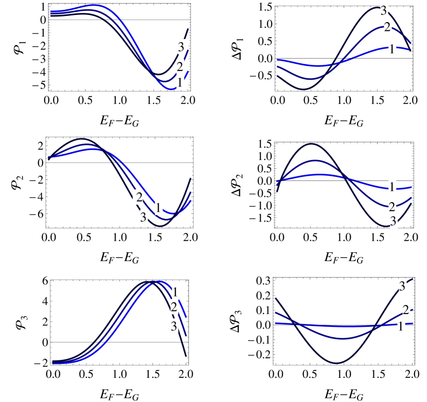
Figure 4: (Color online) Exchange interaction energies ${\cal P}_{1}$ (top panel), ${\cal P}_{2}$ (middle panel) and ${\cal P}_{3}$ (bottom panel) on the left column, as well as the changes of them $\Delta{\cal P}_{1}$ (top panel), $\Delta{\cal P}_{2}$ (middle panel) and $\Delta{\cal P}_{3}$ (bottom panel) on the right column, in doped graphene as functions of the Fermi energy $E_{F}-E_{g}$ for fixed $R_{AA}=R_{BB}=R_{AB}=1.0$. Curves $1,\,2,\,3$ correspond to the gap energy parameter $E_{g}=0.1,\,0.3,\,0.5$ respectively. Here, we measure energy in units of $\gamma_{0}$ and distance in units of $R_{\mu\nu}=|\textbf{r}_{\mu}-\textbf{r}^{\prime}_{\nu}|/a$ for $\mu,\,\nu=A,\,B$.

Figure 4 presents the calculated results for ${\cal P}_{j}(E_{g},R_{\mu\nu})$ (left column) and $\Delta{\cal P}_{j}(E_{g},R_{\mu\nu})$ (right column) as functions of $E_{F}-E_{g}$ with $R_{AA}=R_{BB}=R_{AB}=1$ and various values of $E_{g}$ in doped graphene. From the left column of this figure, as predicted before RKKYG5 we find that the band-filling introduces an oscillation between positive (ferromagnetic) and negative (antiferromagnetic) signs in ${\cal P}_{1}$, ${\cal P}_{2}$ and ${\cal P}_{3}$. In addition, the zeros (non-magnetic) in ${\cal P}_{1}$, ${\cal P}_{2}$ and ${\cal P}_{3}$ are shifted leftward by increasing the values of $E_{g}$. From $\Delta{\cal P}_{1}$, $\Delta{\cal P}_{2}$ and $\Delta{\cal P}_{3}$ displayed in the right column of this figure, we further discover that the magnitude of such oscillations is enhanced significantly in the presence of an energy gap for a graphene layer.

We exhibit in Fig. 5 our numerical results for $R_{\mu\nu}^{2}{\cal P}_{j}(E_{g},R_{\mu\nu})$ (left column) and $R_{\mu\nu}^{2}\Delta{\cal P}_{j}(E_{g},R_{\mu\nu})$ (right column) as functions of the distance $R_{\mu\nu}$ between two magnetic impurities with $E_{F}-E_{g}=1$ and various values of $E_{g}$ in doped graphene. From the left column of this figure, we find that both positive intra-SI exchange interactions ${\cal P}_{1}$ and ${\cal P}_{2}$ decrease with $R_{\mu\mu}$ but the increase of $E_{g}$ suppresses (enhances) ${\cal P}_{1}$ (${\cal P}_{2}$), respectively. The mixed $1/R^{2}_{\mu\mu}$ and $1/R^{3}_{\mu\mu}$ dependence in ${\cal P}_{1,2}(E_{g},R_{\mu\nu})$, as predicted in Ref. [RKKYG5, ] for doped graphene, is modified dramatically. This clearly demonstrates the gap modulation of the doping effect on the intra-SI indirect exchange interaction between magnetic impurities in graphene. Moreover, ${\cal P}_{3}$ is found to increase with $R_{AB}$ with a negligible effect from $E_{g}$, which is accompanied by a switching from antiferromagnetic (negative) to ferromagnetic (positive) beyond a threshold distance between a pair of magnetic impurities in the inter-SI exchange interaction. From the right-hand column of this figure, we find that these exists a negative minimum (positive maximum) for the gap-induced change $\Delta{\cal P}_{1}$ ($\Delta{\cal P}_{2}$) as a function of $R_{\mu\mu}$, respectively. Interestingly, the gap-induced change $\Delta{\cal P}_{3}$ for the inter-SI exchange interaction shows up a sign change with increasing $R_{AB}$ for all chosen finite values of $E_{g}$.

IV Concluding Remarks

The RKKY interaction between a pair of magnetic impurities located on lattice sites of monolayer half-filled gapped graphene is theoretically investigated based on the lattice Green’s function formalism. In contrast with the case for gapless monolayer graphene, the RKKY interaction in gapped graphene possesses distinctive properties. Our numerical results in Fig. 3 showed that although the presence of a gap does not change the ferromagnetic nature of the interaction within a chosen sublattice, it introduces an asymmetry between these two sublattices. We find that the larger the band gap, the smaller is the ferromagnetic energy for one of the two sublattices and the opposite behavior for another sublattice at the same time. The antiferromagnetic interaction is also reduced as the gap is increased for undoped graphene but not for doped graphene. Moreover, we found the gap modulation to the distance dependence of the RKKY interaction for both undoped ($1/R^{3}$) and doped (mixed $1/R^{2}$ and $1/R^{3}$) graphene, where $R$ is the distance between two magnetic impurities on sublattice sites. Additionally, we showed that the doping-induced oscillations in the magnetization within a sublattice or between sublattices can be substantially modified by an energy gap in both magnitude and phase. Some time ago, Gumbs and Glasser Gumbs-Glasser showed that the RKKY interaction in a metal is modified by the presence of a surface and its long-distance behavior is not given by a simple power law as in the bulk. The results in the present paper again confirm that the RKKY interaction may be significantly influenced by chemical composition or the local environment of the material.

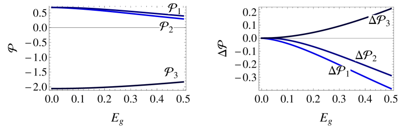
Figure 1: (Color online) Exchange interaction energies ${\cal P}_{1}$, ${\cal P}_{2}$ and ${\cal P}_{3}$ (left panel), as well as the changes of them $\Delta{\cal P}_{1}$, $\Delta{\cal P}_{2}$ and $\Delta{\cal P}_{3}$ (right panel), in undoped graphene as functions of the half-gap $E_{g}$ for fixed $R_{AA}=R_{BB}=R_{AB}=0.5$. Here, we measure energy in units of $\gamma_{0}$ and distance in units of $R_{\mu\nu}=|\textbf{r}_{\mu}-\textbf{r}^{\prime}_{\nu}|/a$ for $\mu,\,\nu=A,\,B$.

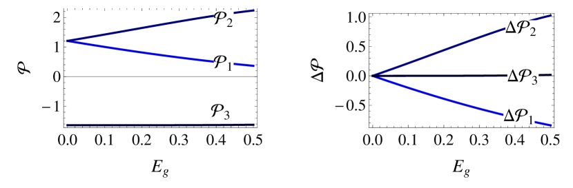
Figure 3: (Color online) Exchange interaction energies ${\cal P}_{1}$, ${\cal P}_{2}$ and ${\cal P}_{3}$ (left panel), as well as the changes of them $\Delta{\cal P}_{1}$, $\Delta{\cal P}_{2}$ and $\Delta{\cal P}_{3}$ (right panel), in doped graphene as functions of the half-gap $E_{g}$ for fixed $R_{AA}=R_{BB}=R_{AB}=1$ and $E_{F}-E_{g}=1$. Here, we measure energy in units of $\gamma_{0}$ and distance in units of $R_{\mu\nu}=|\textbf{r}_{\mu}-\textbf{r}^{\prime}_{\nu}|/a$ for $\mu,\,\nu=A,\,B$.

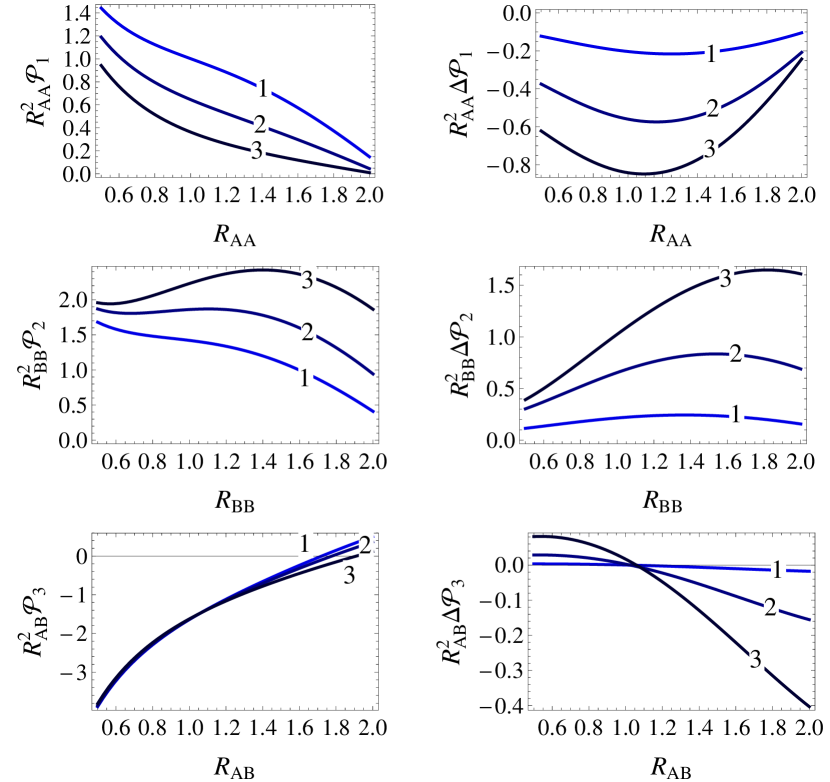
Figure 5: (Color online) Exchange interaction energies $R^{2}_{AA}{\cal P}_{1}$ (top), $R^{2}_{BB}{\cal P}_{2}$ (middle) and $R^{2}_{AB}{\cal P}_{3}$ (bottom) on the left column, as well as the changes of them $R^{2}_{AA}\Delta{\cal P}_{1}$ (top), $R^{2}_{BB}\Delta{\cal P}_{2}$ (middle) and $R^{2}_{AB}\Delta{\cal P}_{3}$ (bottom) on the right column, in doped graphene at $E_{F}-E_{g}=1$ as functions of the distance between two magnetic impurities. Curves $1,\,2,\,3$ correspond to gap energy parameter $E_{g}=0.1,\ 0.3,\ 0.5$, respectively. Here, we measure energy in units of $\gamma_{0}$ and distance in units of $R_{\mu\nu}=|\textbf{r}_{\mu}-\textbf{r}^{\prime}_{\nu}|/a$ for $\mu,\,\nu=A,\,B$.

- (1) M. A. Ruderman and C. Kittel, Phys. Rev. 96, 99 (1954).
- (2) T. Kasuya, Prog. Theor. Phys. 16, 45 (1956).
- (3) K. Yosida, Phys. Rev. 106, 893 (1957).
- (4) E. Kogan, Phys. Rev. B 84, 115119 (2011).
- (5) B. Uchoa, T. G. Rappoport, and A. H. Castro Neto, Phys. Rev. Lett. 106, 016801 (2011).
- (6) M. Sherafati and S. Satpathy, Phys. Rev. B 83, 165425 (2011).
- (7) A. M. Black-Schaffer, Phys. Rev. B 81, 205416 (2010).
- (8) L. Brey, H. A. Fertig, and S. Das Sarma, Phys. Rev. Lett. 99, 116802 (2007).
- (9) S. Saremi, Phys. Rev. B 76, 184430 (2007).
- (10) V. K. Dugaev, V. I. Litvinov, and J. Barnas, Phys. Rev. B 74, 224438 (2006).
- (11) M. A. H. Vozmediano, M. P. Lopez-Sancho, T. Stauber, and F. Guinea, Phys. Rev. B 72, 155121 (2005).
- (12) P. K. Pyatkovskiy, J. Phys.: Condens. Matt. 21, 025506 (2009).
- (13) S. Y. Zhou, G-H. Gweon, A. V. Fedorov, P. N. First, W. A. de Heer, D-H. Lee, F. Guinea, A. H. Castro Neto, and A. Lanzara, Nat. Mater. 6, 770 (2007).
- (14) G. Li, A. Luican and E. Y. Andrei, 2008 arXiv:0803.4016
- (15) O. V. Kibis, Phys. Rev. B 81, 165433 (2010).
- (16) O. Roslyak, G. Gumbs, S. Mukamel, J. Chem. Phys. 136, 194106 (2012).
- (17) A. Iurov, G. Gumbs, O. Roslyak, and D. H. Huang, J. Phys.: Condens. Matt. 24, 015303 (2012).
- (18) D. Huertas-Hernando, F. Guinea, and A. Brataas, Phys. Rev. B 74 155426 (2006).
- (19) Y. Yao, F. Ye, X-L. Qi, S-C. Zhang, and Z. Fang, Phys. Rev. B 75, 041401 (2007).
- (20) G. Gumbs and M. L. Glasser, Phys. Rev. B 33, 6739 (1986).