High Power Microwave and Optical Volume Free Electron Lasers (VFELs)

Abstract

The use of a non-one-dimensional distributed feedback, arising through Bragg diffraction in spatially periodic systems (natural and artificial (electromagnetic, photonic) crystals), forms the foundation for the development of volume free electron lasers (VFELs). The present review addresses the basic principles of VFEL theory and describes the promising potential of VFELs as the basis for the development of high-power microwave and optical sources.

1 Introduction

Research and development of microwave generators using radiation from an electron beam in a periodic slow–wave circuit (traveling–wave tube, backward wave oscillator, etc.) has a long history (see e.g. [1, 2, 3]). One of the characteristic features of such generators is the use of distributed feedback (DFB) where the electromagnetic waves produced by the electron beam are collinear with the direction of the beam motion (one-dimensional distributed feedback; see Fig. 1).

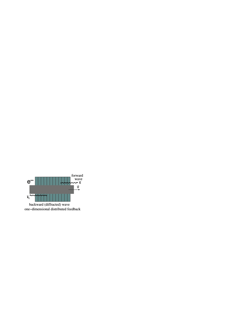
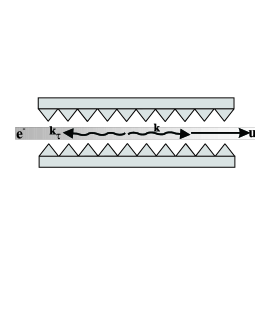
Figure 1:

It is well known that every radiating system is defined by its eigenmodes and by the so-called dispersion equation, which describes the relation between the frequency $\omega$ and the wave vector $\vec{k}$ ($\omega=\omega(\vec{k})$ or $\vec{k}=\vec{k}(\omega)$). A thorough analysis of the dispersion equation shows that:

1. dispersion equation for a FEL [4] in the Compton regime coincides with that for a conventional traveling wave tube amplifier (TWTA);

2. FEL gain (increment of electron beam instability) in the Compton regime is proportional to $n_{0}^{1/3}$, where $n_{0}$ is the electron beam density.

It was first shown in [5, 6] that the law of electron beam instability can change significantly under the conditions of a non-one-dimensional distributed feedback formed in a two– or three–dimensional periodic resonator (natural or artificial (electromagnetic, photonic) crystal); see Fig. 2.

Figure 2:

It was shown that the gain of electromagnetic waves changes sharply in the vicinity of the points where the roots of the dispersion equation coincide. In particular, according to [5, 6], in the case when the DFB in a spatially periodic resonator is formed by the two waves participating in the Bragg diffraction, the increment of instability is proportional to $n_{0}^{1/4}$. If the DFB is formed by $N$ number of waves (as a result of Bragg diffraction $s=N-1$ number of extra waves are produced (see Fig. 3)), then the increment of instability appears to be proportional to $n_{0}^{\frac{1}{3+s}}$, provided that the roots of the dispersion equation coincide (e.g., for two–wave Bragg diffraction, $N=2$ and $s=1$, for three–wave diffraction, $N=3$ and $s=2$ ).

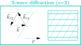
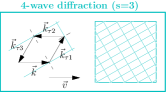
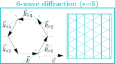
Figure 3:

This result is also valid for electron beams moving in vacuum near the surface of a spatially periodic medium, in a vacuum slot made inside a periodic medium, or between the diffraction gratings of the resonator. The explicit expressions for the starting current $j$ were obtained for the conditions of a non-one-dimensional DFB, and it was shown that the threshold currents in this case can be sharply reduced.

The advantages of VFEL are pronounced in a wide spectral range – from microwaves to X-rays [5, 6, 7, 8, 9, 10].

Providing the capabilities for frequency tuning, using wide electron beams (several e-beams), and reducing the threshold current density, required to initiate lasing, VFELs offer a more promising potential for the development of more compact, high-power and tunable radiation sources than conventional electron vacuum devices.

In particular, experimental investigation of the properties of electromagnetic crystals formed by periodically spaced dielectric threads (wires) demonstrates that the quality factor of such structures can be as high as $\sim 10^{6}\div 10^{8}$ [9]. First experiments have been performed on exciting generation in different types of periodic structures (resonators made of diffraction gratings with two different periods, resonators based on a photonic crystal formed by metallic wires and foils) (for details, see [7]).

Let us note that in [11, 12, 13], published some years after [5, 6], the authors, considering a particular case of using a two-dimensional DFB for the synchronization of radiation across a wide sheet electron beam, also came to the conclusion that such distributed feedback can be used for developing microwave generators.

Benefits given by VFELs:

1. volume FELs provide frequency tuning by rotation of the diffraction grating;

2. use of a non-one-dimensional DFB reduces the generation threshold and the size of the generation zone. It appeared that if $N=1+s$ number of waves participate in the formation of a non-one-dimensional DFB, then there are $N$ number of connected waves propagating in the electromagnetic (photonic) crystal (see Fig.3 ). This set of $N$ number of connected waves has $N$ number of stationary states characterized by wave numbers $k_{i}(\omega)$, ($i=1,...N$). If the relationship $(k_{i}-k_{j})L=2\pi m_{ij}$ ($m_{ij}$ are the integers, which in the general case are not the same) between these waves holds, then a significant change in the threshold current value is possible. Let us note that in the case of a one-dimensional DFD (see Fig. 1), these conditions transform into the requirement for the efficiency of a one-dimensional DFB [15];

3. VFELs allow the use of a wide electron beam (or several beams) and diffraction gratings of large volumes. Two- or three-dimensional diffraction gratings (artificial crystals, now often called the electromagnetic or photonic crystals) allow distributing the interaction over a large volume and overcoming the power restrictions on resonators (see Fig. 2);

4. VFELs can simultaneously generate radiation at several frequencies;

5. VFELs enable effective mode selection in oversized systems, where the radiation wave length is significantly smaller than the resonator dimensions;

6. use of electromagnetic (photonic) crystals with a spatially variable period allows increasing the efficiency of lasing [7, 14].

2 Radiative instability of beams moving in a spatially periodic non-one-dimensional resonator (two- or three-dimensional electromagnetic (photonic) crystal)

Let a relativistic electron beam of velocity $\vec{u}$ enter the resonator having a form of a photonic crystal with length $L$ (the $z$-axis is perpendicular to the crystal surface). Let this photonic crystal have infinite transverse dimensions (crystal plate) and lie in the interval ($0<z<L$). The set of equations describing the interaction of electromagnetic waves with the ”crystal-beam” system consists of Maxwell’s equations and the equations of particle motion in the electromagnetic field. The dielectric susceptibility of a crystal has the form $\varepsilon(\vec{r};\omega)=\sum_{\vec{\tau}}\varepsilon_{\tau}(\omega)\exp(-i\vec{\tau}\vec{r})$, where $\vec{\tau}$ is the reciprocal lattice vector, $\varepsilon_{\tau}$ is the Fourier expansion coefficient of $\varepsilon(\vec{r},\omega)$ and $\varepsilon(\vec{r},\omega)=1+\chi(\vec{r},\omega)$, where $\chi(\vec{r},\omega)$ is the space-periodic crystal polarizability, $\chi(\vec{r},\omega)=\sum_{\tau}\,\chi_{\tau}e^{-i\vec{\tau}\,\vec{r}}$. We assume here for simplicity that $\varepsilon(\vec{r},\omega)$ is the scalar function. For concretness, let us further assume that radiation is excited by quasi-Cherenkov (diffraction) radiation (for details, see [7, 8]). We also let $|\chi_{\tau}\ll 1|$. Perturbations of the current and charge densities in the linear field approximation may be written in the form:

$$\delta\vec{j}(\vec{k};\omega)=e\sum\limits_{\alpha}\exp(-i\vec{k}\vec{r}_{\alpha 0})\left\{\delta\vec{v}_{\alpha}(\omega-\vec{k}\vec{u})-i\vec{u}[\vec{k}\delta\vec{r}_{\alpha}(\omega-\vec{k}\vec{u})]\right\}\delta n(\vec{k};\omega)$$

$$=e\sum\limits_{\alpha}\exp(-i\vec{k}\delta\vec{r}_{\alpha 0})\left\{-i[\vec{k}\vec{r}_{\alpha}(\omega-\vec{k}\vec{u})]\right\}.$$ (1)

Here $\delta\vec{j}(\vec{k};\omega)$ and $\delta n(\vec{k};\omega)$ are the Fourier transformations of the expressions

$$\vec{j}(\vec{r};t)=e\sum\limits_{\alpha}\vec{v}_{\alpha}(t)\delta[\vec{r}-\vec{r}_{\alpha}(t)]\qquad\mbox{and}\qquad n(\vec{r};t)=\sum\limits_{\alpha}\delta[\vec{r}-\vec{r}_{\alpha}(t)]\,;$$

$\vec{u}$ is the unperturbed electron (positron) velocity; $\delta\vec{v}_{\alpha}$ and $\delta\vec{r}_{\alpha}$ are perturbations of the velocity and radius vectors, respectively, arising due to the interaction with the radiation field:

$$\vec{v}_{\alpha}(t)=\vec{u}+\delta\vec{v}_{\alpha}(t)\qquad\vec{r}_{\alpha}(t)=\vec{r}_{\alpha 0}+\vec{u}t+\delta\vec{r}_{\alpha}(t).$$

The subscript $\alpha$ denotes the number of the particle.

Using the equation of particle motion and formula (2) for current density, one can obtain a set of Maxwell’s equations that describes the interaction of electromagnetic waves and particles in crystals:

$$k^{2}_{\tau}\vec{E}(\vec{k}_{\tau^{\prime}},\omega)-\vec{k}_{\tau^{\prime}}[\vec{k}_{\tau^{\prime}}\vec{E}(\vec{k}_{\tau^{\prime}},\omega)]-\frac{\omega^{2}}{c^{2}}\sum\limits_{\tau}\varepsilon_{\tau}(\vec{k}_{\tau^{\prime}},\vec{\omega})\vec{E}(\vec{k}_{\tau+\tau^{\prime}},\omega)$$

$$=-\frac{\omega^{2}_{L}}{\gamma c^{2}}\vec{E}(\vec{k}_{\tau^{\prime}},\omega)-\left(\frac{\omega^{2}_{L}\vec{k}_{\tau^{\prime}}}{\gamma c^{2}(\omega-\vec{k}_{\tau^{\prime}}\vec{u})}+\frac{\omega^{2}_{L}(\vec{k}_{\tau^{\prime}}C^{2}-\omega^{2})}{\gamma C^{4}(\omega-\vec{k}_{\tau^{\prime}}\vec{u})^{2}}\right)$$

$$\times\left[(\vec{u}\vec{E}(\vec{k}_{\tau^{\prime}},\omega))-\left(\frac{\omega^{2}_{L}\vec{u}}{\gamma c^{2}(\omega-\vec{k}_{\tau^{\prime}}\vec{u})}\right)(\vec{k}_{\tau^{\prime}}\vec{E}(\vec{k}_{\tau^{\prime}},\omega))\right],$$

$$\vec{\tau}\,^{\prime}=0,\vec{\tau}_{1},\vec{\tau}_{2},...,\qquad\vec{k}_{\tau}=\vec{k}+\vec{\tau}\,.$$ (2)

The set of equations (2) describes a situation when the DFB is formed by many diffracted waves (note that in the absence of an electron beam, the case of multi-wave diffraction was studied in detail; see e.g. [16]). However, the analysis of such a general situation is very complicated, and so here we consider only a two-wave distributed feedback. This allows us to obtain all the main characteristics of VFELs analytically and show the advantages of non-one-dimensional geometry of distributed feedback over the one-dimensional one.

So let us consider specifically the generation of a $\sigma$-polarized wave (the wave with the polarization vector orthogonal to the diffraction plane, i.e., the plane where vectors $\vec{k}$ and $\vec{\tau}$ lie) for the geometry of the so-called two-beam Bragg diffraction [17], where two strong waves are excited, and diffraction occurs by the set of crystallographic planes, determined by the reciprocal lattice vector  $\vec{\tau}$ (see Figs 4, 5). In this case, the set of Maxwell’s equations, describing two-wave diffraction in crystals traversed by the beam, can be written as

$$\left(k^{2}c^{2}-\omega^{2}\varepsilon_{0}+\frac{\omega^{2}_{L}}{\gamma}+\frac{\omega^{2}_{L}}{\gamma}\frac{(\vec{u}\vec{e}\,^{\prime}_{\sigma})^{2}}{c^{2}}\frac{k^{2}c^{2}-\omega^{2}}{(\omega-\vec{k}\vec{u})^{2}}\right)E_{\sigma}-\omega^{2}\varepsilon_{\tau}E_{\sigma}^{\tau}=0$$

$$-\omega^{2}\varepsilon_{-\tau}E_{\sigma}+\left(K^{2}_{\tau}c^{2}-\omega^{2}\varepsilon_{0}+\frac{\omega^{2}_{L}}{\gamma}+\frac{\omega^{2}_{L}}{\gamma}\frac{(\vec{u}\vec{e}_{\sigma})^{2}}{e^{2}}\frac{k^{2}_{\tau}c^{2}-\omega^{2}}{(\omega-\vec{k}_{\tau}\vec{u})^{2}}\right)\vec{E}_{\sigma}^{\tau}=0.$$

In equation (2), $E_{\sigma}=\vec{E}(\vec{k},\omega)\cdot\vec{e}_{\sigma}$, $E_{\sigma}^{\tau}=\vec{E}(\vec{k}+\vec{\tau},\omega)\cdot\vec{e}_{\sigma}$, $\vec{e}_{\sigma}\parallel[\vec{k}\vec{\tau}]$, and $\omega^{2}_{L}=4\pi e^{2}n_{0}/m$, where $n_{0}$ is the average electron density in the beam. According to (2), the system ”crystal-particle beam” may be considered as an active medium with dielectric susceptibility

$$\tilde{\varepsilon}_{0}(\vec{k},\omega)-1=\varepsilon_{0}-1-\frac{\omega^{2}_{L}}{\gamma\omega^{2}}-\frac{\omega^{2}-L}{\gamma\omega^{2}}\frac{(\vec{u}\vec{e}_{\sigma})^{2}}{c^{2}}\frac{k^{2}c^{2}-\omega^{2}}{(\omega-\vec{k}\vec{u})^{2}},\leavevmode\nobreak\ \tilde{\varepsilon}_{\tilde{\tau}}=\varepsilon_{\tau}=\chi_{\tau}$$

$$\tilde{\varepsilon}_{0}(\vec{k}_{\tau},\omega)-1=\varepsilon_{0}-1-\frac{\omega^{2}_{L}}{\gamma\omega^{2}}-\frac{\omega^{2}_{L}}{\gamma\omega^{2}}\frac{(\vec{u}\vec{e}_{\sigma})^{2}}{c^{2}}\frac{\vec{k}^{2}_{\tau}c^{2}-\omega^{2}}{(\omega-\vec{k}_{\tau}\vec{u})^{2}},\leavevmode\nobreak\ \tilde{\varepsilon}_{-\tau}=\varepsilon_{-\tau}=\chi_{-\tau}$$

Further, we shall analyze the generation of a wave with wave vector $\vec{k}$, making a small angle with the particle velocity vector $\vec{u}$. In this case, the wave vector $\vec{k}_{\tau}=\vec{k}+\vec{\tau}$ is directed at a large angle relative to $\vec{u}$, and consequently the magnitude of $(\omega-\vec{k}_{\tau}\vec{u})$ cannot become small. As a result, the terms containing the expression $(\omega-\vec{k}_{\tau}\vec{u})$ in their denominators will be small and can be ignored. We shall also neglect the term $\omega^{2}_{L}/\gamma$ – this is justified for real beam densities.

It is well known that the equation set (2) has nonzero solutions when its determinant equals zero. This defines the dispersion equation, which can be written in the form

$$(\omega-\vec{k}\vec{u})^{2}\left[(k^{2}c^{2}-\omega^{2}\varepsilon_{0})(k^{2}_{\tau}c^{2}-\omega^{2}\varepsilon_{0})-\omega^{4}\varepsilon_{\tau}\varepsilon_{-\tau}\right]=$$ (4)

$$-\frac{\omega^{2}_{L}}{\gamma}\frac{(\vec{u}\vec{e}_{\sigma})^{2}}{c^{2}}(k^{2}c^{2}-\omega^{2})(k^{2}_{\tau}c^{2}-\omega^{2}\varepsilon_{0}).$$

Dispersion equation (4) yields the relationship for $\omega=\omega(\vec{k})$ or $\vec{k}=\vec{k}(\omega)$.

3 Generation equations and threshold conditions in the case of two-wave Bragg diffraction

In order to determine the structure of the fields and describe the instability evolution in the systems, one needs to know the dispersion equations and their solutions, as well as the boundary conditions.

Now we shall formulate the boundary problem. Let an electron beam with mean velocity $\vec{u}$ be incident onto a plane-parallel spatially periodic plate of thickness $L$. The electron beam is oriented so that it generates radiation under Bragg diffraction conditions. Under two-wave diffraction, two fundamentally different geometries are possible.

In the first case (Laue geometry (see Fig.4), both waves are emitted through one and the same boundary of the periodic structure ($\gamma_{0}=\frac{{\left({\vec{k}\vec{n}}\right)}}{{k}}>0$ and $\gamma_{1}=\frac{{\left({\vec{k}_{\tau}\vec{n}}\right)}}{{k}}>0$, here $\vec{n}$ is the unit normal vector to the entrance surface).

Figure 4: Geometry of two-wave Laue diffraction; $\vec{k},\vec{k}_{\tau}$ are the wave vectors of the incident and diffracted waves, respectively, and $\vec{\tau}$ is the reciprocal lattice vector of the periodic structure. The projections of both wave vectors onto the direction of the normal to the surface have the same sign.

In the second case (Bragg geometry, see Fig. 5), the incident and diffracted waves leave the plate through the opposite surfaces ($\gamma_{0}>0$ and $\gamma_{1}<0$).

Figure 5: Geometry of two-wave Bragg diffraction; $\vec{k},\vec{k}_{\tau}$ are the wave vectors of the incident and diffracted waves, respectively and $\vec{\tau}$ is the reciprocal lattice vector of the periodic structure. The projection of the wave vectors onto the direction of the normal to the surface are opposite in sign.

Let us consider the Bragg case in more detail

The general solution for the field in a crystal is written as

$$\vec{E}=\sum\limits_{i=1}^{4}\vec{e}_{\sigma}c_{i}\exp(i\vec{k_{i}}\vec{r})[1+s_{i}\exp(i\vec{\tau}\vec{r})],$$ (5)

where $\vec{k}_{i}$ is the i-th solution to dispersion equation (4) and $\vec{k}_{i\tau}=\vec{k}_{i}+\vec{\tau}$, with $\vec{\tau}$ being the reciprocal lattice vector corresponding to the planes of diffraction reflection. In writing (5), we used four roots of dispersion equation (4), instead of six. Two roots can be discarded because at $|\chi_{\tau}|\ll 1$, mirror-reflected waves can be ignored.

The boundary conditions, necessary for defining the fields in a crystal, may be written as [7, 8]

$$c_{1}+c_{2}+c_{3}+c_{4}=1,$$

$$f_{1}c_{1}+f_{2}c_{2}+f_{3}c_{3}+f_{4}c_{4}=0,$$

$$g_{1}c_{1}+g_{2}c_{2}+g_{3}c_{3}+g_{4}c_{4}=0,$$ (6)

$$s_{1}c_{1}e^{iK_{1z}L}+s_{2}c_{2}e^{iK_{2z}L}+s_{3}c_{3}e^{iK_{3z}L}+s_{4}c_{4}e^{iK_{4z}L}=0,$$

$$s_{i}=\frac{\omega^{2}\varepsilon_{-\tau}}{k^{2}_{i_{\tau}}c^{2}-\omega^{2}\varepsilon_{0}},\qquad f_{i}=\frac{(\vec{u}\vec{e}_{\sigma})^{2}}{(\omega-\vec{k}_{i}\vec{u})},\qquad g_{i}=\frac{k^{2}_{i}c^{2}-\omega^{2}}{(\omega-\vec{k}_{i}\vec{u})^{2}}\frac{(\vec{u}\vec{e}_{\sigma})^{2}}{c^{2}}.$$

The first equation in (3) corresponds to the continuity of the incident wave at the boundary $z=0$ (the wave incident on the crystal is assumed to have a unit amplitude). The last equation in (3) reflects the fact that behind the crystal, no waves move in the diffraction direction (they appear due to diffraction in space before the entrance surface of the crystal; the general case, which is true for both Bragg and Laue geometries, is considered in [7]). Here $i=1\div 4$ are the solutions to dispersion equation (4). The second and the third conditions correspond to the continuity of the beam density and the beam current density at the crystal entrance. Here we apply the expressions obtained from the equations of particle motion and the expression for the particle beam current

$$\delta j_{\sigma}=\frac{ie^{2}n_{0}}{m\gamma\omega}\frac{(\vec{u}\vec{e}_{\sigma})^{2}}{c^{2}}\frac{k^{2}c^{2}-\omega^{2}}{(\omega-\vec{k}\vec{u})^{2}}E_{\sigma}$$

$$j_{\sigma}=e(\vec{u}\vec{e}_{\sigma})n_{0}-\frac{ie^{2}n_{0}}{m\gamma}\frac{(\vec{u}\vec{e}_{\sigma})^{2}}{c^{2}(\omega-\vec{k}\vec{u})}E_{\sigma}.$$ (7)

The linear system (3), defining the coefficients $c_{i}$, has the solution $c_{i}=\Delta_{i}/\Delta$, where $\Delta$ is the determinant of the system (3) and $\Delta_{i}$ is the $i$-th minor, obtained as a result of replacement of the $i$-th column by

$$\left(\begin{array}[]{c}1\\ 0\\ 0\\ 0\end{array}\right).$$

Hence, at $\Delta\rightarrow 0$, the field amplitudes inside the crystal increase, and as a result, the field in the crystal is nonzero, even when the amplitude of the incident wave vanishes. The condition $\Delta=0$ with $\Delta_{i}\neq 0$ is called the generation threshold condition [18]. Substituting the expressions

$$\vec{k}_{i}=\vec{k}_{0}+\vec{k}\delta_{i}\vec{n},\qquad k_{0z}=\frac{\omega-\vec{k}_{\perp}\vec{u}_{\perp}}{u_{z}},$$

$$k=\omega/c,\qquad\delta_{i}\ll 1,$$ (8)

(where $\vec{n}$ is the normal to the crystal surface and $\vec{k}_{0}=(k_{0z},\vec{k}_{\perp})$) into the determinant $\Delta$, we can represent the generation threshold condition $\Delta=0$ as

$$\frac{(\delta_{1}-\delta_{2})(\delta_{1}-\delta_{3})(\delta_{2}-\delta_{3})}{\delta_{1}^{2}\delta_{2}^{2}\delta_{3}^{2}}s_{4}e^{ik\delta_{4}L}-\frac{(\delta_{1}-\delta_{2})(\delta_{1}-\delta_{4})(\delta_{2}-\delta_{4})}{\delta_{1}^{2}\delta_{2}^{2}\delta_{4}^{2}}s_{3}e^{ik\delta_{3}L}$$ (9)

$$+\frac{(\delta_{1}-\delta_{3})(\delta_{1}-\delta_{4})(\delta_{3}-\delta_{4})}{\delta_{1}^{2}\delta_{3}^{2}\delta_{4}^{2}}s_{2}e^{ik\delta_{2}L}-\frac{(\delta_{2}-\delta_{3})(\delta_{2}-\delta_{4})(\delta_{3}-\delta_{4})}{\delta_{2}^{2}\delta_{3}^{2}\delta_{4}^{2}}s_{1}e^{ik\delta_{1}L}=0\,.$$

In eq. (9), the terms containing nonresonant $f_{i}$ and $g_{i}$ ($i=1\div 4$) were neglected.

Upon solving (9), one may determine the threshold generation conditions, i.e., the values of the electron current and other parameters of the beam, at which radiation begins to exceed the losses [7, 8].

In the case of low-gain regime, for instance, the formula for the generation threshold under the conditions of two–wave diffraction was obtained in the form [8]:

$$-\frac{\pi^{2}n^{2}}{4\gamma}\left(\frac{\omega_{L}}{\omega}\right)^{2}k^{3}L_{*}^{3}\left(\chi_{0}^{\prime}+|\chi_{\tau}|/\sqrt{-\beta}-\gamma^{-2}\right)\left(\chi_{0}^{\prime}+|\chi_{\tau}|/\sqrt{-\beta}\right)\sin^{2}\varphi\times f(y)$$

$$=\left(\frac{\gamma_{0}c}{\vec{u}\vec{n}}\right)^{3}\frac{16(-\beta)\pi^{2}n^{2}}{(k|\chi_{\tau}|L_{*})^{2}}+k\chi_{0}^{\prime\prime}L_{*}\left(\frac{1}{\sqrt{-\beta}}-1\right)^{2}.$$ (10)

Here $\omega$ is the radiation frequency; $\omega_{L}=\sqrt{4\pi e^{2}n_{0}/m_{e}}$ is the Langmuir frequency of the beam; $n_{0}$ is the average electron density in the beam; $e$ and $m_{e}$ are the electron charge and mass, respectively; $\gamma$ is the beam Lorentz factor; $L_{*}=Lu/(\vec{u}\,\vec{n})$ is the distance traveled by the beam in the crystal; $\vec{u}$ is the unperturbed velocity vector of the beam particles; $\vec{n}$ is the unit normal vector to the crystal surface (directed toward the interior); $L$ is the crystal thickness; $\chi_{0}$ and $\chi_{\tau}$ are the Fourier expansion coefficients of the crystal dielectric susceptibility (their real and imaginary parts are denoted by prime and double prime, respectively); $\beta=\gamma_{1}/\gamma_{0}$ is the diffraction asymmetry factor; $\gamma_{0}$ and $\gamma_{1}$ are the cosines of the angles between the normal vector $\vec{n}$ and the wave vectors of the transmitted $\vec{k}$ and diffracted $\vec{k}+\vec{\tau}$ waves, respectively; $\varphi$ is the angle between the vectors $\vec{k}_{\perp}$ and $\vec{\tau}_{\perp}$ (here the subscript $\perp$ denotes the projection of the vector on the plane perpendicular to $\vec{u}$); $n$ is the integer; $f(y)$ is the spectral function depending on detuning from the synchronism conditions:

$$f(y)=\sin y\frac{(2y+\pi n)\sin y-y(y+\pi n)\cos y}{y^{3}(y+\pi n)^{3}},$$ (11)

where $y=kx_{2}^{\prime}L/2$ and $x_{2}$ is the root of the dispersion equation in the absence of the electron beam:

$$x_{1,2}=a\pm\sqrt{a^{2}+b}\,.$$ (12)

Here

$$a = -\frac{1}{4}(l/\gamma_{0}+l_{\tau}/\gamma_{1})\,,\qquad b=-\frac{1}{4\gamma_{0}\gamma_{1}}(ll_{\tau}-\chi_{\tau}\chi_{-\tau})\,,$$

$$l = \theta^{2}-\chi_{0}+\gamma^{-2}\,,\qquad\quad l_{\tau}=l+\alpha\,,$$

where $\theta$ is the angle between the vectors $\vec{k}$ and $\vec{u}$ and $\alpha=\vec{\tau}(2\vec{k}_{0}+\vec{\tau})/k_{0}^{2}$ characterizes deviation from the exact Bragg condition.

Let us note that (10) is obtained in the vicinity of the condition imposed on the phase difference between the waves in the crystal

$$\texttt{Re}\,(k_{1z}-k_{2z})L=2\pi n,$$ (13)

which in the considered case has the form

$$kL\sqrt{a^{2}+b}=\pi n.$$ (14)

and it is assumed that the following inequalities hold:

$$k|\chi_{\tau}|L\gg 1\,,\qquad|\chi_{\tau}|\ll 1\,,\qquad|\chi_{0}|\ll 1\,.$$

The condition (10) has a clear physical meaning: the left-hand side of (10) contains the term describing generation of radiation by the electron beam, and the right-hand side includes the terms describing losses at the boundaries (the first term) and absorption losses (the second term) in the medium. It is obvious that if the absorption is small, then at fixed values of $y$ (e.g. if $y=0$, then f(y)=1), eq. (10) yields the following dependence of the threshold generation current on the target length (the left-hand side of (10) is proportional to $\omega_{L}^{2}\sim n_{0}$, i.e., $\sim j$):

$$j_{th}\sim\frac{1}{(kL_{*})^{5}}.$$ (15)

It also follows from (10) that the value of the threshold current in the case of a non-one-dimensional DFB depends appreciably on the parameter $\beta$ and the effective photon path length $L_{*}$ in the resonator (recall that $L_{*}=L\,u/(\vec{u}\vec{n})$).

4 VFEL based on an electromagnetic undulator

Similar considerations enable finding generation thresholds for the beams moving in an electromagnetic undulator [19, 20, 21].

Let an electron beam move with average velocity $\vec{u}_{0}$ through a two- or three-dimensional periodic medium (electromagnetic (photonic) crystal) placed in an external field. Vector potential of the external field can be written as

1. $$\vec{A}=A_{w}\vec{x}\sin k_{w}z\qquad\mbox{(a magnetostatic wiggler)}\,,$$

   where $A_{w}=B_{w}/k_{w}$, $k_{w}=2\pi/\lambda_{w}$, and $\vec{x}\cdot\vec{u}_{0}=0$, with $B_{w}$ being the magnetic field strength and $\lambda_{w}$ being the wiggler wavelength ($\vec{x}$, $\vec{y}$, and $\vec{z}$ are the unit vectors of the Cartesian coordinate system)($c=1$);

2. $$A=A_{em}\vec{x}\sin(\vec{k}_{em}\vec{r}-\omega_{em}t)\,,$$

   where $A_{em}=E_{em}/\omega_{em}$. Here $E_{em}$ is the amplitude of the electric field of the electromagnetic wave and $\omega_{em}$, $\vec{k}_{em}$ are its frequency and wave vector, respectively. The external field excites oscillations of electrons, having the transverse velocity $\vec{v}_{\perp}=e\vec{A}/m\gamma$, where $\gamma=(1-v^{2})^{-1/2}$ is the Lorentz factor of the electron. A moving oscillator emits electromagnetic radiation, whose frequency $\omega$ and wave vector $\vec{k}$ satisfy the condition of synchronism:

   $$\noindent\omega-\vec{k}\vec{u}_{\parallel}=\Omega,\Omega=\left\{\begin{array}[]{l}\vec{k}_{w}\vec{u}_{\parallel}\quad(\mbox{for a magnetic wiggler})\,,\\ \\ \omega_{em}-\vec{k}_{em}\vec{u}\quad(\mbox{for an electromagnetic wiggler})\,,\end{array}\right.$$ (19)

   where the longitudinal velocity of the electron $u_{\parallel}=u_{0}\left(1-\frac{a^{2}_{w}}{\gamma^{2}}\right)$ (the corresponding longitudinal Lorentz factor $1/\gamma^{2}_{\parallel}=(1+a^{2}_{w})/\gamma^{2}$, $a_{w}=eA_{w}/m$ is the undulator parameter; $k=n(\omega)\omega$, $k_{em}=n(\omega_{em})\omega_{em}$, and $|n(\omega)-1|\ll 1$). We shall further consider the case of forward scattering.

Let us write Maxwell’s equation in the Fourier space in the two-wave approximation of the dynamical diffraction theory (when the Bragg condition is satisfied only for one reciprocal lattice vector). For the field of $\sigma$-polarization, we have:

$$[k^{2}-\omega^{2}(1+\chi_{0})]E-\omega^{2}\chi_{-\tau}E_{\tau}=4\pi i\omega j\,,$$ (20)

$$-\omega^{2}\chi_{\tau}E+[k_{\tau}^{2}-\omega^{2}(1+\chi_{0})]E_{\tau}=4\pi i\omega j_{\tau}\,,$$ (21)

where $E=\vec{E}(\vec{k},\,\omega)\cdot\vec{e}_{\sigma}$ and $E_{\tau}=\vec{E}(\vec{k}_{\tau}\,,\omega)\cdot\vec{e}_{\sigma}$ are the Fourier components of the electromagnetic field of $\sigma$-polarization, $\vec{k}_{\tau}=\vec{k}+\vec{\tau}$, $\vec{e}_{\sigma}=\vec{k}\times\vec{k}_{\tau}/|\vec{k}\times\vec{k}_{\tau}|$ is the $\sigma$-polarization unit vector, $j=\vec{j}(\vec{k}\,,\omega)\cdot\vec{e}_{\sigma}$ and $j_{\tau}=\vec{j}(\vec{k}_{\tau}\,,\omega)\cdot\vec{e}_{\sigma}$ are the projections of the Fourier components of the current density vector onto the $\sigma$-polarization unit vector, and $\chi_{0}$ and $\chi_{\tau}$ are the Fourier components of the periodic tensor of crystal polarizability.

Let us use the linear approximation for solving the equations

$$\frac{\partial f}{\partial t}+\vec{v}\frac{\partial f}{\partial\vec{r}}+\frac{\partial\vec{p}}{\partial t}\,\frac{\partial f}{\partial\vec{p}}=0\,,\qquad\frac{\partial\vec{p}}{\partial t}=e(\vec{E}+\vec{v}\times\vec{B})\,.$$ (22)

In this case, we can write

$$f(\vec{r}\,,\vec{p}\,,t)=f_{0}(\vec{p})+\delta f(\vec{r}\,,\vec{p}\,,t),\quad\delta f\sim E,\quad\delta f\ll f_{0}\,.$$ (23)

From (22) and (23) follows

$$\left(\frac{\partial}{\partial t}+\vec{v}\frac{\partial}{\partial\vec{r}}\right)\delta f+\frac{\partial\vec{p}}{\partial t}\,\frac{\partial f_{0}}{\partial\vec{p}}=0\,.$$ (24)

In the equation of motion (24) and the expression $\vec{j}=e\int\vec{v}f(\vec{r}\,,\vec{p}\,,t)d^{3}p$ for the current density, we shall go over to the Fourier components. Let us express the perturbation of the distribution function in (24) in terms of $E(\vec{k}\,,\omega)$ and then substitute it into (20) and (21). If the beam’s velocity distribution $v_{th}$ satisfies the relationships $\vec{k}\cdot\vec{v}_{th}\ll\Omega$ and $\vec{k}\cdot\vec{v}_{th}\ll\vec{\tau}\cdot\vec{u}$, then one can obtain the dispersion equation in the form:

$$D_{0}(\vec{k},\omega)=-4\pi e^{2}\omega(k^{2}_{\tau}-\omega^{2}(1+\chi_{0}))\frac{a^{2}_{w}}{\gamma^{2}}I\,,$$

$$D_{0}(\vec{k},\omega)=(k^{2}-\omega^{2}(1+\chi_{0}))(k^{2}_{\tau}-\omega^{2}(1+\chi_{0}))-\omega^{4}\chi_{\tau}\chi_{-\tau}\,,$$ (25)

$$I=\int\frac{df_{0}}{dp}\,\frac{dp}{\vec{k}\vec{u}_{\parallel}-\omega+\Omega}\,,\qquad p=\vec{p}\cdot\vec{s}\,,\qquad\vec{s}=\frac{\vec{u}_{\parallel}}{u_{\parallel}}\,.$$ (26)

Let a crystal have a form of a plane-parallel plate of thickness $L$, then $L_{*}$ denotes the particle path length in the crystal (see Sec. 3). Here we shall consider only the case of weak amplification, when $k^{\prime\prime}L_{*}\ll 1$, with $k^{\prime\prime}$ being the imaginary part of the solution to dispersion equation (4). There are two characteristic limiting cases for which (4) can be reduced to the algebraic equation.

1. If the inequality

   $$\vec{k}\vec{v}_{th}\ll 1/L_{*}$$ (27)

   is fulfilled, then we can neglect the beam dispersion and set the initial distribution function to be $f_{0}(p)=n_{0}\delta(p-p_{0})$, where $n_{0}$ is the beam’s spatial density. As a result, we can write the dispersion equation for a cold-beam regime.

   $$D_{0}(\vec{k}\,,\omega)(\omega-\vec{k}\vec{u}_{\parallel}-\Omega)^{2}=-2\omega^{4}(k^{2}_{\tau}-\omega^{2}(1+\chi_{0}))F\,.$$ (28)

   Here $F=\frac{\omega^{2}_{p}a_{w}^{2}}{2\gamma^{3}\gamma^{3}_{\parallel}\omega^{2}}$ and $\omega^{2}_{p}=\frac{4\pi e^{2}n_{0}}{m}$ is the plasma frequency of the beam.

2. If inequality (29), inverse to (27), is fulfilled:

   $$\vec{k}\vec{v}_{th}\gg 1/L_{*}\,,$$ (29)

   then we can speak of a ”hot” beam regime. To evaluate the integral in (26), we use the Gaussian distribution function $f_{0}(p)=\frac{n_{0}}{\sqrt{\pi}p_{th}}e^{-(p-p_{0})^{2}/p^{2}_{th}}$ and obtain the dispersion equation in the ”hot” beam regime:

   $$D_{0}(\vec{k}\,,\omega) = -2\omega^{2}(k^{2}_{\tau}-\omega^{2}(1+\chi_{0}))\frac{F}{v^{2}_{th}}\,\frac{2}{\sqrt{\pi}}\left(1+i\sqrt{\pi}\frac{u_{f}-u_{\parallel 0}}{v_{th}}\right)\,,$$ (30)

   $$u_{f} = \left\{\begin{array}[]{l}\frac{\omega}{k_{\parallel}+k_{w}}\,\mbox{(for a magnetic wiggler)}\,,\\ \frac{\omega-\omega_{em}}{k_{\parallel}+k_{em}}\quad\mbox{(for an electromagnetic wiggler)}\,.\end{array}\right.$$

4.1 Boundary Conditions

Let a wave vector of the incident wave be $\vec{k}_{0}=\omega\vec{s}$. From the continuity of the wave field at the boundary follows that inside the crystal, the wave vector $\vec{k}=\vec{k}_{0}+\omega\delta\vec{n}$ ($\delta\ll 1$ because $|\chi_{0}|$, $|\chi_{\tau}|\ll 1$). Let us introduce the following notations: $\gamma_{0}=\vec{k}_{0}\cdot\vec{n}/\omega$, $\gamma_{1}=(\vec{k}_{0}+\vec{\tau})\cdot\vec{n}/\omega$, $\beta_{1}=\gamma_{0}/\gamma_{1}$, $\alpha=((\vec{k}_{0}+\vec{\tau})^{2}-\omega^{2})/\omega^{2}$, $\chi_{1}=\chi_{0}-\alpha$, $\varepsilon=\gamma_{0}\delta$, and $\xi=-\frac{1}{2\gamma^{2}_{\parallel}}-\frac{F}{\omega}$ and recast dispersion equations (28), (30) in a more convenient form:

$$(\varepsilon-\varepsilon_{1}^{(0)})(\varepsilon-\varepsilon_{2}^{(0)})(\varepsilon-\varepsilon_{k})=-\left(\varepsilon+|\beta_{1}|\frac{\chi_{1}}{2}\right)F\,,$$ (33)

$$(\varepsilon-\varepsilon_{1}^{(0)})(\varepsilon-\varepsilon_{2}^{(0)})=-\left(\varepsilon+|\beta_{1}|\frac{\chi_{1}}{2}\right)\frac{F}{v^{2}_{th}}\,\frac{2}{\sqrt{\pi}}\,\left(1+i\sqrt{\pi}\frac{(u_{f}-u_{0})}{v_{th}}\right)\,,$$ (34)

$$\varepsilon_{1}^{(0)}=\frac{1}{4}\left[\chi_{0}-|\beta_{1}|\chi_{1}+\sqrt{(\chi_{0}+|\beta_{1}|\chi_{1})^{2}-4|\beta_{1}|\chi_{\tau}\chi_{-\tau}}\right]\,,$$

$$\varepsilon_{2}^{(0)}=\frac{1}{4}\left[\chi_{0}-|\beta_{1}|\chi_{1}-\sqrt{(\chi_{0}+|\beta_{1}|\chi_{1})^{2}-4|\beta_{1}|\chi_{\tau}\chi_{-\tau}}\right]\,.$$ (35)

In writing (33) and (34), we have taken into account that in the case of Bragg geometry considered here (the diffracted wave leaves the crystal through the entrance surface), $\beta_{1}<0$. The general solution describing scattering of the external wave with the field strength $\vec{E}=E_{0}\vec{x}e^{i(\vec{k}_{0}\vec{r}-\omega t)}$ by the system ”crystal-beam” is as follows:

$$\vec{E}=\vec{x}e^{i(\vec{k}_{0}\vec{r}-\omega t)}\sum_{j=1}^{N}(E_{j}+e^{i\vec{\tau}\vec{r}}E_{\tau j})e^{i\varepsilon_{j}\omega z/\gamma_{0}}\,,$$ (36)

and, according to (21), $\vec{E}_{\tau j}=\vec{E}_{j}\frac{\chi_{\tau}}{2\varepsilon_{j}+|\beta_{1}|\chi_{1}}$; $N=4$ and $N=2$ for a ”cold” and a ”hot” beam, respectively. To determine the amplitudes of the fields inside the crystal, the boundary conditions must be used. In Bragg geometry, they are as follows:

1. the continuity of field $E$ at the entrance boundary

   $$\sum_{j=1}^{N}E_{j}=E_{0}\,,$$ (37)

2. the continuity of field $E_{\tau}$ at the exit boundary

   $$\sum_{j=1}^{N}\frac{E_{j}e^{i\varepsilon_{j}\omega L}}{\varepsilon_{j}+|\beta_{1}|\frac{\chi_{1}}{2}}=0\,,$$ (38)

3. the continuity of the beam’s density at the entrance boundary

   $$\int\delta fdp|_{z=0}=0\,,$$ (39)

4. the continuity of the beam’s current density at the entrance boundary

   $$\int u\delta fdp|_{z=0}=0\,.$$ (40)

Using the expression for the Fourier components $df$, which follows from (24), let us express (39) and (40) in terms of the amplitude $E_{j}$ in the crystal. It can be shown that for the case of a ”cold” beam, expressions (39) and (40) yield the equations:

$$\sum_{j=1}^{4}\frac{E_{j}}{\xi-\varepsilon_{j}}=0\,,\qquad\sum_{j=1}^{4}\frac{E_{j}}{(\xi-\varepsilon_{j})^{2}}=0\,.$$ (41)

These equations, together with equations (37) and (38), give four independent conditions that are necessary to define the four amplitudes $E_{j}$ of the field. For a ”hot” beam, both of the conditions (39) and (40) can be reduced to (37), i.e., only the conditions (37) and (38) are independent and sufficient for defining the two amplitudes of the field. Let $g_{ij}$ denote the elements of the fundamental matrix of the system (37), (38), and (41). The boundary conditions enable one to determine the field amplitudes, which can be written in the form $E_{j}=E_{0}\bar{g}_{j1}/G$, where $\bar{g}_{j1}$ is the cofactor of the element $g_{j1}$, and $G=\det\|g_{i1}\|$. If $G$ vanishes, then the amplitudes $E_{j}$ in the crystal can be nonzero, even when the amplitude $E_{0}$ of the external incident field equals zero. This correlates with the phenomenon of self-excitation (generation), arising due to the existence of the distributed feedback. On this account, we shall call the equation $G=0$ the generation condition. Calculating the determinant of the matrix $\|g_{i}j\|$, one can reduce the generation condition to the form:

$$\sum_{j=1}^{4}\frac{e^{i(\varepsilon_{j}-\xi)\omega L}(\varepsilon_{j}-\xi)^{2}}{\left(\varepsilon_{j}+|\beta_{1}|\frac{\chi_{1}}{2}\right)\prod_{i\neq j}(\varepsilon_{i}-\varepsilon_{j})}=0$$ (42)

for a ”cold” beam and

$$\frac{e^{i\varepsilon_{1}\omega L_{*}}}{\varepsilon_{1}+|\beta_{1}|\frac{\chi_{1}}{2}}=\frac{e^{i\varepsilon_{2}\omega L_{*}}}{\varepsilon_{1}+|\beta_{1}|\frac{\chi_{1}}{2}}$$ (43)

for a ”hot” beam.

4.2 Generation Thresholds

Recall that the Fourier components of crystal polarizability have the form:

$$\chi_{0}=-|\chi_{0}^{\prime}|+i|\chi_{0}^{\prime\prime}|\,,\quad\chi_{\pm\tau}=-|\chi_{\pm\tau}^{\prime}|+i|\chi_{\pm\tau}^{\prime\prime}|\,,\quad|\chi_{0}^{\prime\prime}|\,,|\chi_{\pm\tau}^{\prime\prime}|\ll|\chi_{0}^{\prime}|\,,|\chi_{\tau}^{\prime}|.$$

Now, let us analyze the case when

$$\sqrt{|\chi_{0}^{\prime\prime}|\,|\chi_{\tau}^{\prime}|}\ll\varepsilon_{1}^{(0)}-\varepsilon_{2}^{(0)}\ll|\chi_{\tau}^{\prime}|\,.$$ (44)

As is seen from (4.1), this occurs at small deviations from $\alpha\simeq\frac{1}{|\beta_{1}|}(\pm 2\sqrt{|\beta_{1}|}|\chi_{\tau}^{\prime}|-|\chi_{0}^{\prime}|(1+|\beta_{1}|))$, i.e., in the vicinity of the absorption edges. The solutions to (33) at $\texttt{Re}\,\varepsilon_{1}^{(0)}=\xi$ or $\texttt{Re}\,\varepsilon_{2}^{(0)}=\xi$ are of particular interest and correspond to the synchronism between the beam and one of the DFB resonator modes. In Table I, the possible cases are labelled with numbers and letters for convenience.

Table 1:

Synchronism condition	$\alpha=\frac{1}{|\beta_{1}|}\left(2\sqrt{|\beta_{1}|}|\chi^{\prime}_{\tau}|-|\chi^{\prime}_{0}|(1+|\beta_{1}|)\right)$	$\alpha=\frac{1}{|\beta_{1}|}\left(-2\sqrt{|\beta_{1}|}|\chi^{\prime}_{\tau}|-|\chi^{\prime}_{0}|(1+|\beta_{1}|)\right)$
$\texttt{Re}\,\varepsilon_{1}^{(0)}=\xi$	1a)	2a)
$\texttt{Re}\,\varepsilon_{2}^{(0)}=\xi$	1b)	2b)

In cases 1a) and 2b), equation (42) does not have a solution.

The condition (42) can be satisfied when the following equalities hold:
in case 1b)

$$\frac{F(\omega L_{*})^{3}}{8\pi n}=\omega\left(|\chi_{0}^{\prime\prime}|\frac{(1+|\beta_{1}|)}{2}-|\chi_{\tau}^{\prime\prime}|\sqrt{|\beta_{1}|}\right)L_{*}+\frac{8\pi^{2}n^{2}}{\omega^{2}\chi_{\tau}L_{*}^{2}}\,;$$ (45)

in case 2a)

$$\frac{F(\omega L_{*})^{3}}{8\pi n}=\omega\left(|\chi_{0}^{\prime\prime}|\frac{(1+|\beta_{1}|)}{2}+|\chi_{\tau}^{\prime\prime}|\sqrt{|\beta_{1}|}\right)L_{*}+\frac{8\pi^{2}n^{2}}{\omega^{2}\chi_{\tau}L_{*}^{2}}\,.$$ (46)

Let us recall that $F=\frac{\omega^{2}_{p}a_{w}^{2}}{2\gamma^{3}\gamma^{3}_{\parallel}\omega^{2}}$. The solutions to (43) in the case of a ”hot” beam have the form

1. $$\omega\frac{F}{v^{3}_{th}}(u_{\parallel\,0}-u_{f})L_{*} = \omega\left(|\chi_{0}^{\prime\prime}|\frac{(1+|\beta_{1}|)}{2}-|\chi_{\tau}^{\prime\prime}|\sqrt{|\beta_{1}|}\right)L_{*}+\frac{8\pi^{2}n^{2}}{\omega^{2}\chi_{\tau}L_{*}^{2}}\,,$$

   $$\alpha = \frac{1}{|\beta_{1}|}\left(2\sqrt{|\beta_{1}|}|\chi^{\prime}_{\tau}|-|\chi^{\prime}_{0}|(1+|\beta_{1}|)\right)\,,$$

   $$n = 1,\,2\,...$$ (47)

2. $$\alpha = \frac{1}{|\beta_{1}|}\left(-2\sqrt{|\beta_{1}|}|\chi^{\prime}_{\tau}|-|\chi^{\prime}_{0}|(1+|\beta_{1}|)\right)\,,$$

   $$\frac{\omega F}{v^{3}_{th}}(u_{\parallel\,0}-u_{f})L_{*} = \omega\left(|\chi_{0}^{\prime\prime}|\frac{(1+|\beta_{1}|)}{2}-|\chi_{\tau}^{\prime\prime}|\sqrt{|\beta_{1}|}\right)L_{*}+\frac{8\pi^{2}n^{2}}{\omega^{2}\chi_{\tau}L_{*}^{2}}\,,$$

   $$n = 1,\,2\,...$$ (48)

Since $F\sim\omega_{p}^{2}\sim n_{0}\sim j$, the value of the threshold current can be found using equations (45)–(2).

Again, we have $j_{th}\sim\frac{1}{L_{*}^{5}}$ for a ”cold” beam. Equations (45)–(2) are the amplitude conditions of generation. To satisfy the generation conditions, one more condition must be fulfilled - the phase condition, common for all the cases:

$$\texttt{Re}\,\varepsilon_{1}^{(0)}-\varepsilon_{2}^{(0)}=2\pi n/\omega L_{*}\,.$$ (49)

The condition (49) leads to the fact that the longitudinal structure of the eigenmodes $|E|^{2}$ and $|E_{\tau}|^{2}$ appears to be close in form to a standing wave. Thus, this condition is similar to a well-known condition of standing wave formation in a mirror resonator.

Formulas (45)–(2) are similar in form. On the left-hand sides, they contain the gain of the free electron laser in the appropriate mode. Their right-hand sides describe the losses related to energy absorption in crystals and its leakage through the boundaries of a DFD resonator.

It should be noted that in view of the above, the value of the threshold current in the case of a non-one-dimensional DFB depends appreciably on the parameter $\beta_{1}$ and the effective photon path length $L_{*}$ in the resonator (recall that $L_{*}=L\,u/(\vec{u}\vec{n})$).

Let us consider the equation defining the threshold conditions for backward Bragg diffraction ($|\beta|,|\beta_{1}|=1$ and $\vec{u}\parallel\vec{n}$). In this case, we go over to a one-dimensional DFB. The implicit form of the equation for the threshold current was obtained in [22] (see eq. (10) in [22]). From this equation, one can also derive the expressions for the threshold current. To do this, let us take eqs. (9) and (10), derived in [22], and substitute eq. (9) for the quality factor $Q$ into eq. (10). Then we can write

$$(CL^{\prime})^{3}\varphi^{\prime}(\Phi)=\frac{2\pi^{2}n^{2}}{(\sigma L^{\prime})^{2}},$$ (50)

where $n$ is the integer; $L^{\prime}$ is the dimensionless length of the structure, e.g., the waveguide with shallow corrugations ($L^{\prime}=\frac{\omega}{c}L$); $\sigma$ is the so-called wave coupling coefficient due to corrugations, whose physical meaning is similar to that of the quantity $\chi_{\tau}$. Here $C=(eI\kappa^{2}\mu/m\gamma\omega^{2}N_{s})^{1/3}$ is the generalized Pierce parameter, where $I$ is the current of the electron beam, $\kappa$ is the coupling coefficient between the direct wave and and the electron beam, $\mu$ is the electron bunching parameter, and $N_{s}$ is the norm of the wave in a smooth wavequide. In (50), $\Phi=-\Gamma_{e}L^{\prime}$, where $\Gamma_{e}=-(\Delta+\delta)$. Here $\Delta=(\omega-\omega_{B})/\omega_{B}\approx(h-h_{B})/h_{B}$ is detuning from the exact Bragg condition; $h_{B}=\pi/d$, $\omega_{B}=c\sqrt{g^{2}+h_{B}^{2}}$, $d$ is the corrugation period, $h$ and $g$ are the longitudinal and transversal wavenumbers, respectively, and $\delta$ is the resonance detuning between the synchronous wave and the electrons.

The function $\varphi^{\prime}(\Phi)$ has the form:

$$\varphi^{\prime}(\Phi)\equiv\frac{d}{d\Phi}\left\{2\pi^{2}n^{2}\frac{1-(-1)^{n}\cos\Phi}{(\Phi^{2}-\pi^{2}n^{2})^{2}}\right\}\,.$$ (51)

Now let us write the explicit form of the derivative of $\varphi^{\prime}(\Phi)$

$$\varphi^{\prime}(\Phi)=2\pi^{2}n^{2}\frac{(-1)^{n}\sin\Phi(\Phi^{2}-\pi^{2}n^{2})-4\Phi(1-(-1)^{n}\cos\Phi)}{(\Phi^{2}-\pi^{2}n^{2})^{3}}\,.$$ (52)

At first glance, the spectral functions in (11) and (51) differ. It can be shown, however, that virtually they are one and the same function, but of different arguments. Indeed, in the case of a symmetric backward Bragg diffraction, we have $\beta\approx-1$, and the quantity $a$ in (12) is $a=\alpha/4\approx\Delta$. Then assuming that $\delta=0$ and considering the condition (14), we get $2y\approx\Phi+\pi n$. Substituting this equality for the arguments into (51), we obtain $\varphi^{\prime}(\Phi)=\varphi^{\prime}(2y+\pi n)=-\frac{\pi^{2}n^{2}}{4}f(y)$. Thus the condition (50) takes the form:

$$-\frac{\pi^{2}n^{2}}{4}(CL^{\prime})^{3}f(y)=\frac{2\pi^{2}n^{2}}{(\sigma L^{\prime})^{2}},$$ (53)

which is equivalent to (10) (note, however, that in (53), the radiation absorption is ignored). Recalling that $C^{3}\sim I$, we immediately obtain that the condition (53) yields the same dependence of the threshold current density on $L$ as in eq. (10).

We may note in conclusion that in contrast to a one-dimensional case, where Laue geometry does not occur, in a non-one-dimensional case it occurs along with the generation in Bragg geometry. A more detailed analysis of the radiation process in Laue geometry can be found in [7] and the references there.

5 Generation equations and threshold conditions in the geometry of three-wave Bragg diffraction

Above, we have discussed the theory of the volume distributed feedback formation in the geometry of a non-one-dimensional two-wave Bragg diffraction. Let us proceed now to the consideration of multi-wave DFB in a two(three)-dimensional periodic resonator. Multi-wave DFB arises when $N$ number of waves simultaneously satisfy the conditions of Bragg diffraction.

Use of multi-wave Bragg diffraction in a VFEL for the formation of a volume distributed feedback enables one, on the one hand, to appreciably reduce the length of the generation area (at a given operating current) or the operating current (at a given length of the generation area), and on the other hand, to apply electron beams with a large transverse cross section (or several electron beams) for generating radiation, which improves the electrical endurance of the generator.

Application of multi-wave diffraction for generating in a microwave range has one more remarkable feature – the possibility of selecting modes in oversized waveguides and resonators.

Production of high-power microwave pulses requires high electric strength of the generator and radiation resistance of the output window. To reduce the load on these elements, the transversal (with respect to the direction of the electron beam velocity) dimension of the resonator should be large (much larger than the wavelength). As a rule, this leads to a multi-mode generation regime and low efficiency. When $N$ number of waves are diffracted, the modes can be effectively selected due to the requirement to satisfy the Bragg condition $N-1$ .

To illustrate the potential of multi-wave distributed feedback, let us consider three-wave diffraction in more depth (for details, see Section 13 in [7]). In this case, the distributed feedback can be realized in three different geometries:

(1) Laue-Laue diffraction when the three waves exit through the same surface ($\gamma_{0},\gamma_{1},\gamma_{2}>0$, here $\gamma_{i}$ is the cosine of the angle between the wave vector $\vec{k}_{i}$ and the normal to the crystal surface (see e.g. [16]); Fig. 6);

Figure 6: Three-wave diffraction in Laue-Laue geometry. Projections of wave vectors $\vec{k},\vec{k}_{\tau 1}$, and $\vec{k}_{\tau 2}$ onto the surface normal $\vec{n}$ have the same sign; $\vec{\tau}_{1}$ and $\vec{\tau}_{2}$ are the reciprocal lattice vectors of the periodic structure.

(2) diffraction in Bragg-Bragg geometry when $\gamma_{0}>0$, while $\gamma_{1},\gamma_{2}<0$;

(3) Bragg-Laue diffraction when $\gamma_{0},\gamma_{1}>0$, and $\gamma_{2}<0$; see Figure 7.

Figure 7: Three-wave diffraction in Laue-Bragg geometry. Projections of wave vectors $\vec{k}$ and $\vec{k}_{\tau 1}$ onto the surface normal are opposite in sign to the projection of vector $\vec{k}_{\tau 2}$; $\vec{\tau}_{1}$ and $\vec{\tau}_{2}$ are the reciprocal lattice vectors of the periodic structure.

Similarly to the two-wave case, the problem of the beam interaction with the resonator (photonic crystal) can be reduced to the problem of three-wave diffraction of an electromagnetic wave incident onto the active medium. The active medium here is the system ”spatially–periodic structure + electron beam”.

The dependence of the threshold conditions on the length of the interaction area at the point of threefold degeneration changes appreciably

$$G=A\chi_{0}^{\prime\prime}+\frac{{B}}{{kL}}\left({\frac{{2\pi}}{{klL}}}\right)^{4}\,.$$ (54)

Here in the regime of a ”cold” electron beam, $G\sim jL^{2}$, with $j$ being the beam current density. Realization of this regime requires the fulfillment of the phase condition $\left({k_{1z}-k_{2z}}\right)L=2\pi n$, $\left({k_{2z}-k_{3z}}\right)L=2\pi m$, $n\neq m$. The coefficients $A$ and $B$ in (54) depend on the diffraction geometry, the value of $\chi_{\tau}$, and the indices $m$ and $n$. According to (54), for a ”cold” electron beam, when absorption is not important, $j_{\mathrm{thr}}\sim\frac{{1}}{{\left({kL}\right)^{3}}}\left({\frac{{2\pi}}{{klL}}}\right)^{4}$. Under dynamical diffraction, when the inequality $\frac{{4\pi}}{{klL}}\ll 1$ holds, this dependence leads to an appreciable reduction in the threshold current. The analysis shows that when a multi-wave ($N$-wave) DFB is excited, the threshold current depends on $L$ as

$$j_{thr}\sim\frac{1}{\left(kL\right)^{3}}\left(\frac{2\pi}{klL}\right)^{2s}\,,$$ (55)

that is,

$$j_{th}\sim\frac{1}{L^{3+2s}}\,,$$

where $s=N-1$ is the number of extra waves appearing through diffraction in the crystal.

So, the transition to multi-wave diffraction enables one to significantly reduce the operating current and the longitudinal dimensions of the generating system.

As follows from the above results, the volume distributed feedback (non-one-dimensional feedback) has a number of advantages that make its application beneficial for generating stimulated radiation in a wide spectral range (with wavelengths from microwave and optical to angström). Moreover, in a short-wave spectral range, where the requirements for the current density and the quality of the beam are very strict, it becomes possible to noticeably reduce the threshold current for a given beam propagation area. In this case, the VFEL is a unique system providing lasing at relatively small interaction lengths. When producing high-power radiation pulses in oversized generators in a microwave range, VFELs are beneficial for the reduction of the threshold current, generator size, and for mode selection.

6 Use of a dynamical undulator mechanism to produce short wavelength radiation in VFELs

Numerous applications can benefit from the development of powerful electromagnetic generators with frequency tuning in millimeter, sub-millimeter and terahertz wavelength range, using low-relativistic electron beams. Low-relativistic electron beams in the undulator system can be used for radiating in a short-wavelength range, but in this case the undulators period must be small. For example, to obtain radiation with the wavelength of $0.3-1\leavevmode\nobreak\$ mm at the beam energy $E=800$ KeV$-1$ MeV, the undulator period must be $\sim 0.3-1\leavevmode\nobreak\$cm. Development of such undulators is a very complicated task. The use of a two-stage FEL with a dynamical wiggler generated by the electron beam [4] is a possible solution to this problem.

The above-described potentialities to significantly reduce the threshold currents and resonator dimensions by using a non-one-dimensional distributed feedback, which arises due to Bragg diffraction in a two– or three–dimensional spatially-periodic resonator (electromagnetic (photonic) crystal) and serves as a foundation for designing Volume Free Electron Lasers (VFELs), enable the development of two-stage VFELs with a dynamical wiggler generated by electron beams. A dynamical wiggler can be created with the help of any radiation mechanism: Cherenkov, Smith-Purcell, quasi-Cherenkov [8], or undulator. VFEL principles offer the advantage of a two-stage generation scheme and, in particular, allow one to smoothly tune the period of the dynamical wiggler by rotating the diffraction grating. There is a possibility of smooth frequency tuning for both the pump and the signal waves by either varying the geometric parameters of the volume diffraction grating or by rotating the diffraction grating or the beam. Moreover, the VFEL allows one to create a dynamical wiggler in a large volume, which is hard to achieve with a static wiggler.

There are two stages in the generation scheme proposed above (see Section 16, Fig. 16 [7]):

(a) creation of a dynamical wiggler in a system with two-dimensional (three-dimensional) gratings (in other words, during this stage the electromagnetic field, which exists inside the VEFL resonator, is used to create a dynamical wiggler). Smoothly varying the orientation of the diffraction grating in the VEFL resonator, one can smoothly change the dynamical wiggler parameters;

(b) radiation is generated by the electron beam interacting with the dynamical wiggler, which has been created during the previous stage (stage a).
Both stages evolve in the same volume.

7 Conclusion

Thus,

1. volume FELs provide frequency tuning by rotation of the diffraction grating;

2. use of a non-one-dimensional DFB reduces the generation threshold and the size of the generation zone;

3. VFELs allow the use of a wide electron beam (or several beams) and diffraction gratings of large volumes. Two- or three-dimensional diffraction gratings (artificial crystals, now often called the electromagnetic or photonic crystals) allow distributing the interaction over a large volume and overcoming the power restrictions on resonators and thus open up the possibility of developing powerful generators with wide electron beams (or system of beams);

4. VFELs enable effective mode selection in oversized systems, where the radiation wave length is significantly smaller than the resonator dimensions;

5. principles of VFEL can be used for creation of a dynamical wiggler with a variable period in a large volume;

6. two-stage scheme of generation, based on a non-one-dimensional distributed feedback, can be applied for lasing in the teraHertz frequency range using low-relativistic beams;

7. two-stage scheme of generation combined with the volume distributed feedback can also form the basis for the development of powerful generators with wide electron beams (or system of beams);

8. use of a hybrid system composed of several phase-locked vircator arrays generating modulated beams that enter the VFEL resonator enables further increase of the generator’s power output [7, 23]. Moreover, a VFEL resonator composed of periodically-arranged metallic elements aids in preventing the Coulomb repulsion of electrons. The maximum limiting current that can be transmitted through such a resonator is greater than the limiting current that can be transmitted through a vacuum drift space of a conventional BWO or TWT (compare with the methods of increasing the current transmitted through the resonator, suggested in [24, 25, 26]).

   To achieve this, two(three)-dimensional electromagnetic crystals formed by periodically arranged screens with periodically spaced holes for beam transmission can also be used along with those formed by periodically arranged wires, wire arrays and cylinders.

Let us note in conclusion that inverse free electron lasers are known to be used for particle acceleration. Similarly, VFELs with a non-one-dimensional distributed feedback, arising in electromagnetic (photonic) crystals, can be operated in the inverse mode for accelerating particle beams [6]. In this case, the acceleration rate is appreciably higher than that achieved in conventional FELs.

References

• [1] J.R.Pierci. Travelling wave tubes (Van Nostrand, Princeton 1950).
• [2] S.H. Gold and G.S. Nusinovich, Rev. Sci. Instrum. 68, 11 (1997) pp. 3945–3974.
• [3] J. Benford, J.A. Swegle, E. Schamiloglu, High Power Microwaves, 2-nd ed. (Taylor and Francis Group, New York, London, 2007).
• [4] T.C. Marshall, Free-Electron Lasers (Macmillan Publishing Company, London, 1985).
• [5] V.G. Baryshevsky, I.D. Feranchuk, Phys. Lett. A 102 (1984) 141.
• [6] V.G. Baryshevsky, Doklady Akad. Nauk SSSR 299 (1988) 19.
• [7] V. G. Baryshevsky, LANL e-print arXiv:1101.0783 [physics.acc-ph, physics.optics].
• [8] V.G. Baryshevsky, K.G. Batrakov, I.Ya. Dubovskaya Journ. Phys. D 24 (1991) pp. 1250–1257.
• [9] V.G. Baryshevsky, K.G. Batrakov, I.Ya. Dubovskaya, V.A. Karpovich, V.M. Rodionova, Volume quasi-Cherenkov FEL in mm-spectral range, in G. Dattoli and A. Renieri (eds.) Free Electron Lasers (Elsiver Science B.V., 1997) pp. II-75-II-76.
• [10] V.G. Baryshevsky, K.G. Batrakov, I.Ya. Dubovskaya, Nucl. Instrum. Methods A 358 (1995) pp. 493–496.
• [11] N.S. Ginzburg, N.Iu. Peskov, A.S. Sergeev, Pis’ma Zh. Tekh. Fiz. 18, 9 (1992) pp. 23–28 (In Russian).
• [12] N.S. Ginzburg, N.Yu. Peskov, A.S. Sergeev, A.V. Arzhannikov, S.L. Sinitsky, Nucl. Instrum. Methods A 358, 1 3 (1995) pp. 189–192
• [13] N.S. Ginzburg, K.E. Dorfman, A.M. Malkin, A.S. Sergeev, Pis’ma Zh. Tekh. Fiz. 35, 12 (2009) pp. 9–17 (In Russian).
• [14] V.G. Baryshevsky, A.A. Gurinovich, Experimental study of a volume free electron laser with a ”grid” resonator, in Proceedings of FEL2006, Aug. 2006 (Berlin, Germany) p. 335.
• [15] H. Kogelnik and C. Shank, J. Appl. Phys. 43(1972) pp. 2327–2335.
• [16] Chang Shih-Lin, Multiple Diffraction of X-Rays in Crystals (Springer-Verlag Berlin Heidelberg New-York Tokyo, 1984).
• [17] Z. G. Pinsker, Dynamical Scattering of X-rays in Crystals (Springer-Verlag Berlin, Heidelberg, New York, 1978).
• [18] A. Yariv and P. Yeh, Optical Waves in Crystals (Wiley, 1984).
• [19] V.G. Baryshevsky, I.Ya. Dubovskaya, A.V. Zege, Phys. Lett. A 149, 1, (1990) pp. 30–34.
• [20] V.G. Baryshevsky, I.Ya. Dubovskaya, A.V. Zege, Vesti Akad. Nauk. BSSR, ser. fiz.-energ. 3 (1990) pp. 49–56.
• [21] V.G. Baryshevsky, I.Ya. Dubovskaya, A.V. Zege, Nucl. Instrum. Methods B 51 (1990) pp. 368–382.
• [22] V.L. Bratman, N.S. Ginzburg, G.G. Denisov, Sov. Tech. Phys. Lett. 7, 11 (1981) pp. 565–567. (Pis’ma Zh. Tekh. Fiziki 7, 21, (1981) pp. 1320–1324).
• [23] V.G. Baryshevsky, A.A. Gurinovich, LANL e-print arXiv:0903.0300 [physics.acc- ph].
• [24] D.D. Ryutov, Pis’ma Zh. Tekh. Fiziki 1, 12 (1975) pp. 581–584.
• [25] V.K. Grishin, Zh. Tekh. Fiziki 43, 10 (1973) 2209.
• [26] R.A.Richardson, J. Denavit, M. S. Di Capua, and P. W. Rambo, J. Appl. Phys. 69, 9 (1991) pp. 6261–6272.