Analytical and numerical calculations of spectral and optical characteristics of spheroidal quantum dots

Abstract

In the effective mass approximation for electronic (hole) states of a spheroidal quantum dot with and without external fields the perturbation theory schemes are constructed in the framework of the Kantorovich and adiabatic methods. The eigenvalues and eigenfunctions of the problem, obtained in both analytical and numerical forms, were applied for the analysis of spectral and optical characteristics of spheroidal quantum dots in homogeneous electric fields.

I Introduction

Quantum dots(QDs) are considered to be promising as the elementary basis for the new generation of semiconductor devices 1A ; Harrison . The unique opportunity to perform the energy level control and flexible manipulation in QDs is due to the full quantization of charge carrier energy spectra in these systems. This allows design and manufacturing of artificial structures with prescribed quantum physical characteristics 2A . That is why the scope of QDs potential applications is very wide, from heterostructure lasers to nanomedicine and nanobiology. An impressive example of such application is represented by QD lasers possessing low threshold current and high efficiency 2A .

The peculiarities of physical processes in QDs are caused by both their composition and geometry. Electronic, kinetic, optical and other properties of QDs have been investigated experimentally and theoretically in many papers 11A ; LL94 ; Hayk02 ; 79a ; 79 ; 13A ; 14A ; 15 ; Suslov1 ; Suslov2 . Particularly, the optical absorption characteristics of QDs have been shown to be strongly correlated with their geometry, on one hand, and with their physical–chemical properties, on the other hand. In one of the first publications on optical transitions in QD Efros1982 the interband absorption of light was considered in the ensemble of weakly interacting spherical QDs implanted in a dielectric matrix. The dispersion of QD sizes was characterized in the framework of Lifshitz–Slezov theory LS1958 . It was shown that in the absence of size dispersion, due to the full quantization of charge carriers energy spectra in QD, the absorption coefficient behaves like a delta function, and the absorption threshold frequencies depend on the peculiarities of electron and hole energy spectra. When the QD size dispersion is taken into account, the averaging procedure yields the absorption profile having finite width and height.

Recently several reports concerning the experimental implementation of narrow-band InSb QDs have appeared 17A ; 18A , in which the dispersion law for electrons and light holes is non-parabolic and described according to the double-band mirror Kane model Kane ; Askerov . For non-interacting band of heavy holes the dispersion law is considered as quadratic. The investigation of optical absorption peculiarities in InSb QDs with the transitions from light and heavy hole bands to the conduction band taken into account is an interesting problem. Interband transitions in an ensemble of cylindrical or spherical InSb QDs were considered theoretically in the dipole approximation with and without magnetic field, including exciton effects, by means of the perturbation theory and the adiabatic methods20A ; 21A ; Hayk11 . In our earlier work we elaborated the calculation schemes, symbolic-numerical algorithms (SNAs) and programs, based on the generalized Kantorovich method (KM) for numerical solving with required accuracy the boundary-value problems (BVPs) of discrete and continuous spectra describing the axial-symmetric models of quantum wells(QWs), quantum wires(QWrs) and quantum dots(QDs) in external fields within the framework of the effective mass approximation  Yu2 ; CASC10 ; JPCONF ; Yaf10 ; Yaf12 ; kantbp ; ODPEVP ; Yu3 ; Yu4 ; Yu5 ; Yu8 ; Yu9 ; progr07 . Meanwhile, for the analysis and estimations of the appropriate range of material parameters, spectral and optical characteristic of quantum dots at the first stage of investigation, conventionally, approximate eigenvalues and eigenfunctions evaluated in the analytical form were applied  Efros1982 ; Hayk02 ; Hayk11 ; 79 ; 79a . However, it is a real challenge to specify the range of applicability of such approximations in the problems, depending on a few parameters Harrison , e.g., for impurity states of quantum wires in a homogeneous magnetic field  JPCONF .

With this aim in the present paper we report the formulation and MAPLE- environment implementation of algebraic schemes of the perturbation theory (PT) of the Lennard-Jones (LJ) and Rayleigh-Schrödinger (RS) MottSneddon , permissive in the nondiagonal and diagonal adiabatic approximations, respectively, to evaluate in numerical and in analytic forms the eigenvalues and eigenfunctions of models of spheroidal QDs in homogeneous magnetic and electric fields. To construct the required perturbation schemes, we choose such models of spheroidal QDs, in which the basis functions depending upon fast variables can be expressed in the analytic form. The region of the model parameters, for which the PT asymptotic series are applied, is estimated using the results of numerical calculations carried out with required accuracy. The efficiency of the schemes is demonstrated by the analysis of spectral characteristics of oblate and prolate spheroidal QDs and also spherical QDs with corresponding shape of confinement well with walls of infinite height under the influence of homogeneous electric fields (HEFs). We apply the developed approach to the analysis of spectral characteristics of oblate and prolate spheroidal QDs with parabolic and non-parabolic dispersion laws under the influence of HEFs, i.e., the quantum-confined Stark effect.

The paper is organized as follows. In Section 2 the calculation scheme for solving elliptic BVP describing spheroidal QDs in homogeneous electric fields using the Kantorovich method is presented. Section 3 is devoted to the description of the PT schemes by slow variables in nondiagonal adiabatic approximation and the comparison of the results with those of numerical calculation with given accuracy. In section 4 the explicit PT scheme for evaluation of the basis functions of the fast variable for oblate spheroidal QDs in a homogeneous electric field is derived. Section 5 is devoted to the description of PT schemes by slow variables in the diagonal adiabatic approximation for spheroidal QDs in electric fields. The results evaluated here in the analytic form are compared with numerical ones to establish the range of their applicability. In Section 6 the absorption coefficient for an ensemble of spheroidal QDs with random dimensions of minor semiaxis and with parabolic and non-parabolic dispersion laws for holes and electrons under the influence of HEFs is found using the calculated eigenvalues and eigenfunctions. In conclusion we summarize the results and discuss further applications.

II Statement of the problem

Let us consider an impurity localized in the center of a quantum dot and take the electron-hole interaction into account. Then in the effective mass approximation of the ${\bf{k}}\cdot{\bf{p}}$-theory the Schrödinger equation for the slow-varying envelope wave function $\tilde{\Psi}(\tilde{\mathbf{r}_{e}},{\tilde{\mathbf{r}_{h}}})$ of an electron (e) and a hole (h) in a uniform magnetic field $\bf{H}$ with the vector-potential ${\mathbf{A}}=\frac{1}{2}{\mathbf{H}}\times\tilde{{\mathbf{r}}}$ and electric field $\mathbf{F}$ in oblate and prolate QDs reads as 79 :

$$\left\{\tilde{H}(\tilde{\mathbf{r}_{e}},{\tilde{\mathbf{r}_{h}}})-{\tilde{E}}\right\}\tilde{\Psi}(\tilde{\mathbf{r}_{e}},{\tilde{\mathbf{r}_{h}}})=0,$$ (1)

$$\tilde{H}(\tilde{\mathbf{r}_{e}},{\tilde{\mathbf{r}_{h}}})=\sum_{i=e,h}\left\{\frac{1}{2\mu_{i}}\left(\tilde{\hat{\mathbf{p}_{i}}}-\frac{q_{i}}{c}{\mathbf{A}}\right)^{2}-{q_{i}}(\mathbf{F}\cdot\tilde{\mathbf{r}_{i}})+\tilde{U}_{conf}(\tilde{\mathbf{r}_{i}})-\frac{q_{i}q_{c}}{\kappa|{\mathbf{\tilde{r}}_{i}}|}\right\}+\frac{q_{e}q_{h}}{\kappa|{\mathbf{\tilde{r}}_{e}-\mathbf{\tilde{r}}_{h}}|}.$$

Here $\tilde{{\mathbf{r}_{i}}}$ is the radius-vector, $|\tilde{{\mathbf{r}_{i}}}|=\sqrt{\tilde{x_{i}}^{2}+\tilde{y_{i}}^{2}+\tilde{z_{i}}^{2}}$, $\tilde{\hat{{\bf p}_{i}}}=-\imath\hbar\nabla_{\tilde{{\mathbf{r}_{i}}}}$ is the momentum, $\tilde{E}$ is the energy of the particles, $q_{e}=-e$, $q_{h}=+e$, and $q_{c}$ are the Coulomb charges of the electron, the hole, and the impurity center, $\kappa$ is the dc permittivity, $\mu_{i}=\beta_{e(h)}m_{0}$ is the effective mass of electron or hole, $m_{0}$ is the mass of electron. For the model under consideration, $\tilde{U}(\tilde{\bf{r}})$ is the potential of a spherical or axially-symmetric well

$$\tilde{U}(\tilde{{\bf r}_{i}})=\{0,S(\tilde{{\bf r}_{i}})<0;\tilde{U}_{0},S(\tilde{{\bf r}_{i}})\geq 0\},$$ (2)

bounded by the surface $S(\tilde{\bf{r}_{i}})=0$ with walls of infinite height (infinite potential barrier model, IPBM) or finite height $1\ll\tilde{U}_{0}<\infty$ (finite potential barrier model, FPBM). In Eq. (2) $S(\tilde{{\bf r}_{i}})$ depends on the parameters $\tilde{a}$, $\tilde{c}$, which are semiaxes of a spheroidal QD,

$$S(\tilde{{\bf r}_{i}})\equiv({\tilde{x}_{i}^{2}+\tilde{y}_{i}^{2}})/{\tilde{a}^{2}}+{\tilde{z}_{i}^{2}}/{\tilde{c}^{2}}-1.$$ (3)

Below we restrict ourselves to IPBMs of spheroidal quantum dots with possible influence of the uniform electric field ${\bf F}=(0,0,F)$, the magnetic field being switched off, ${\bf H}=0$, and the Coulomb interaction of the electron and the hole with the impurity center being absent, $q_{c}=0$. In this case the wave function $\tilde{\Psi}(\tilde{\mathbf{r}_{e}},{\tilde{\mathbf{r}_{h}}})=\tilde{\Psi}^{e}(\tilde{\mathbf{r}_{e}})\tilde{\Psi}^{h}({\tilde{\mathbf{r}_{h}}})$ is factorized. So, we arrive at the 3D BVPs for unknowns $\tilde{\Psi}^{e}(\tilde{\mathbf{r}_{e}})$ and ${\tilde{E}}^{e}$ or $\tilde{\Psi}^{h}({\tilde{\mathbf{r}_{h}}})$ and ${\tilde{E}}^{h}$. The eigenvalues and eigenfunctions needed to evaluate the absorption coefficients (ACs) were calculated with prescribed accuracy by means of the program packages ODPEVP and KANTBP kantbp ; ODPEVP ; Yu3 . The models with nonzero values of these parameters were announced in JPCONF ; 79 . Throughout the paper we make use of the reduced atomic units Harrison ; LL94 : $a_{B}^{*}={\kappa\hbar^{2}}/{\mu_{p}e^{2}}$ is the reduced Bohr radius, $\tilde{E}_{R}\equiv Ry^{*}={\hbar^{2}}/({2\mu_{p}{a_{B}^{*}}^{2}})$ is the reduced Rydberg unit of energy, and the following dimensionless quantities are introduced: $\tilde{\Psi}(\tilde{\bf r})={a_{B}^{*}}^{-3/2}\Psi({\bf r})$, $2{\hat{H}}=\tilde{\hat{H}}/{Ry^{*}}$, ${\cal E}\equiv 2{E}={\tilde{E}}/{Ry^{*}}$, $2{U({\bf r})}={\tilde{U}(\tilde{\bf r})}/{Ry^{*}}$, ${\bf r}=\tilde{\bf r}/a_{B}^{*}$, $a=\tilde{a}/a_{B}^{*}$, $c=\tilde{c}/a_{B}^{*}$, $2\gamma_{F}=F/F_{0}^{*}$, $F_{0}^{*}=Ry^{*}/(ea_{B}^{*})=e/(2\kappa(a_{B}^{*})^{2})$.

II.1 The BVP for SQDs in the effective mass approximation

In cylindrical coordinates $z,\rho,\varphi$ the solution of Eq. (1), periodical with respect to the azimuthal angle $\varphi$, is sought in the form of a product $\Psi(\rho,z,\varphi)=\Psi^{m}(\rho,z){\exp{(im\varphi)}}/{\sqrt{2\pi}}$, where $m=0,\pm 1,\pm 2,...$ is the magnetic quantum number. The 3D BVP for SQDs at fixed values of $m$ is reduced to 2D BVP with respect to fast $x_{f}$ and slow $x_{s}$ variables: oblate $x_{f}=z$ (minor axis), $x_{s}=\rho$ (major axis) and prolate $x_{f}=\rho$ (minor axis), $x_{s}=z$ (major axis) Yaf12 :

$$\left(\hat{H}_{f}(x_{f};x_{s})+\hat{H}_{s}(x_{s})+{\check{V}_{fs}(x_{f},{x_{s}})}-{{\cal E}_{t}^{m}}\right)\Psi_{t}^{m}(x_{f},x_{s})=0.$$ (4)

Here $\hat{H}_{s}(x_{s})$ is the operator of slow subsystem

$$\hat{H}_{s}(x_{s})=-\frac{1}{g_{1s}(x_{s})}\frac{\partial}{\partial x_{s}}g_{2s}(x_{s})\frac{\partial}{\partial x_{s}}+\check{V}_{s}(x_{s}),$$ (5)

and $\hat{H}_{f}(x_{f};{x_{s}})$ is the operator of fast subsystem

$$\hat{H}_{f}(x_{f};{x_{s}})=-\frac{1}{g_{1f}(x_{f})}\frac{\partial}{\partial x_{f}}g_{2f}(x_{f})\frac{\partial}{\partial x_{f}}+\check{V}_{f}(x_{f};{x_{s}}).$$ (6)

For OSQD $g_{1s}(x_{s})=g_{2s}(x_{s})=1$, $g_{1f}(x_{s})=g_{2f}(x_{s})=\rho$, $\check{V}_{f}(x_{f};{x_{s}})=0$, $\check{V}_{s}(x_{s})=m^{2}/\rho^{2}$, ${\check{V}_{fs}(x_{f},{x_{s}})=2\gamma_{F}z}$, while for PSQD $g_{1s}(x_{s})=g_{2s}(x_{s})=\rho$, $g_{1f}(x_{s})=g_{2f}(x_{s})=1$, $\check{V}_{f}(x_{f};{x_{s}})=m^{2}/\rho^{2}$, $\check{V}_{s}(x_{s})=2\gamma_{F}z$, ${\check{V}_{fs}(x_{f},{x_{s}})=0}$. From (2) the boundary conditions for the eigenfunctions $\Psi_{t}^{m}(x_{f},x_{s})$ of SQDs, corresponding to a well with walls of infinite height, have the form

$$\mathrel{\mathop{\lim}\limits_{\rho\rightarrow 0}}\left(\rho\frac{\partial\Psi^{m}_{t}(\rho,z)}{\partial\rho}\delta_{0m}+\Psi^{m}_{t}(\rho,z)(1-\delta_{0m})\right)=0,\Psi^{m}_{t}(\rho,z)\biggl{|}_{\partial\Omega_{2}}=0,$$

$$\Omega_{2}=\left(\{\rho,z\}\biggl{|}\displaystyle\frac{\rho^{2}}{a^{2}}+\displaystyle\frac{z^{2}}{c^{2}}<1\right),\quad\partial\Omega_{2}=\left(\{\rho,z\}\biggl{|}\displaystyle\frac{\rho^{2}}{a^{2}}+\displaystyle\frac{z^{2}}{c^{2}}=1\right).$$

The eigenfunctions $\Psi_{t}^{m}(x_{f},x_{s})$ corresponding to the eigenvalues ${\cal E}_{t}^{m}={\cal E}_{1}^{m}<{\cal E}_{2}^{m},...$ are subject to the normalization and orthogonality conditions

$$\int_{\Omega_{2}}\rho d\rho dz\Psi_{t}^{m}(\rho,z)\Psi_{t^{\prime}}^{m}(\rho,z)=\delta_{tt^{\prime}}.$$

Note, that at $\gamma_{F}=0$ the solutions are separated by the z-parity $\sigma=\pm 1$ into two invariant subspaces $\Psi_{t}^{m\sigma}$ corresponding to the eigenvalues ${\cal E}_{t}^{m\sigma}={\cal E}_{1}^{m\sigma}<{\cal E}_{2}^{m\sigma},...$ , while at $\gamma_{F}\neq 0$ the z-parity is broken.

II.2 Kantorovich or adiabatic reduction of the BVP

The solution $\Psi_{t}(x_{f},x_{s})\equiv\Psi^{m}_{t}(x_{f},x_{s})$ of the above problem at fixed $m$ is sought in the form of Kantorovich expansion

$$\Psi_{t}(x_{f},x_{s})=\sum_{j=1}^{j_{\max}}B_{j}(x_{f};x_{s})\chi_{jt}(x_{s}).$$ (7)

The set of appropriate trial functions is chosen as the set of eigenfunctions $B_{j}(x_{f};x_{s})$ corresponding to the eigenvalues $\hat{E}_{j}(x_{s})$ of the Hamiltonian $\hat{H}_{f}(x_{f};x_{s})$, Eq. (6), depending parametrically on $x_{s}\in\Omega(x_{s})$:

$$\hat{H}_{f}(x_{f};{x_{s}})B_{j}(x_{f};x_{s})=\hat{E}_{j}(x_{s})B_{j}(x_{f};x_{s}).$$

The eigenfunctions $B_{j}(x_{f};x_{s})$ corresponding to the eigenvalues $\hat{E}_{j}(x_{s})=\hat{E}_{1}(x_{s})<\hat{E}_{2}(x_{s}),...$ are subject to the normalization and orthogonality conditions with the weighting function $g_{1f}(x_{f})$ in the same interval $x_{f}\in\Omega_{x_{f}}(x_{s})$:

$$\int\nolimits_{x_{f}^{\min}(x_{s})}^{x_{f}^{\max}(x_{s})}B_{i}(x_{f};x_{s})B_{j}(x_{f};x_{s})g_{1f}(x_{f})dx_{f}=\delta_{ij}.$$ (8)

The BVP for a set of ODEs of the slow subsystem with respect to the unknown vector functions ${\mbox{\boldmath$\chi$}}_{t}(x_{s})=(\chi_{1;t}(x_{s}),...,\chi_{j_{\max;t}}(x_{s}))^{T}$ corresponding to the unknown eigenvalues $2E_{t}\equiv{\cal E}_{t}$,

$$\biggl{(}\mathbf{D}+{\bf E}({x_{s}})+{\rm{\bf W}}({x_{s}})-{\rm{\bf I}}{\cal E}_{t}\biggr{)}{\mbox{\boldmath$\chi$}}_{t}({x_{s}})=0,$$

$$\mathbf{D}=-\frac{1}{g_{1s}(x_{s})}{\rm{\bf I}}\frac{d}{d{x_{s}}}g_{2s}(x_{s})\frac{d}{d{x_{s}}}+{\rm{\bf I}}\check{V}_{s}(x_{s}),$$ (9)

$${\rm{\bf W}}({x_{s}})={{\rm{\bf U}}({x_{s}})}+\frac{g_{2s}(x_{s})}{g_{1s}(x_{s})}{\rm{\bf H}}({x_{s}})+\frac{1}{g_{1s}(x_{s})}\frac{dg_{2s}(x_{s}){\rm{\bf Q}}({x_{s}})}{d{x_{s}}}+\frac{g_{2s}(x_{s})}{g_{1s}(x_{s})}{\rm{\bf Q}}({x_{s}})\frac{d}{dx_{s}}$$

satisfy the orthogonality and normalization conditions

$$\int\nolimits_{x_{s}^{\min}}^{x_{s}^{\max}}({\mbox{\boldmath$\chi$}}_{t}(x_{s}))^{T}{\mbox{\boldmath$\chi$}}_{t^{\prime}}(x_{s})g_{1s}(x_{s})dx_{s}=\delta_{tt^{\prime}}.$$ (10)

Here the effective potentials $H_{ij}(x_{s})$ and $Q_{ij}(x_{s})$ are defined by the formula

$$U_{ij}(x_{s})=U_{ji}(x_{s})=\int\nolimits_{x_{f}^{\min}(x_{s})}^{x_{f}^{\max}(x_{s})}B_{i}(x_{f};x_{s}){\check{V}_{fs}(x_{f},{x_{s}})}B_{j}(x_{f};x_{s})g_{1f}(x_{f})dx_{f},$$

$$H_{ij}(x_{s})=H_{ji}(x_{s})=\int\nolimits_{x_{f}^{\min}(x_{s})}^{x_{f}^{\max}(x_{s})}\frac{\partial B_{i}(x_{f};x_{s})}{\partial x_{s}}\frac{\partial B_{j}(x_{f};x_{s})}{\partial x_{s}}g_{1f}(x_{f})dx_{f},$$ (11)

$$Q_{ij}(x_{s})=-Q_{ji}(x_{s})=-\int\nolimits_{x_{f}^{\min}(x_{s})}^{x_{f}^{\max}(x_{s})}B_{i}(x_{f};x_{s})\frac{\partial B_{j}(x_{f};x_{s})}{\partial x_{s}}g_{1f}(x_{f})dx_{f}.$$

Here the basis functions of the fast subsystem and the matrix elements are calculated analytically. For oblate spheroidal QDs ($x_{f}=z$, $x_{s}=\rho$)

$$B_{i}\left({x_{f};x_{s}}\right)=B_{i}^{\sigma}\left({x_{f};x_{s}}\right)\!=\!\sqrt{\frac{a}{c\sqrt{{a^{2}}-{x_{s}^{2}}}}}\sin\left(\frac{\pi n_{o}}{2}\left(\frac{x_{f}}{c\sqrt{1-{x_{s}^{2}}/{a^{2}}}}-1\right)\right),$$

$$E_{i}(x_{s})=E_{i}^{\sigma}(x_{s})=E_{i;0}\frac{a^{2}}{(a^{2}-x_{s}^{2})},\quad E_{i;0}=\frac{\pi^{2}i^{2}}{4c^{2}},\quad{U_{ii}(x_{s})=0,}$$ (12)

$${U_{ij}(x_{s})=U_{ij;0}(x_{s})\frac{\sqrt{a^{2}-x_{s}^{2}}}{a},\quad U_{ij;0}(x_{s})=\frac{8\gamma_{F}cij{(-1+(-1)^{i+j})}}{(i^{2}-j^{2})^{2}\pi^{2}},}$$

$$H_{ii}(x_{s})=H_{ii;0}(x_{s})\frac{a^{2}x_{s}^{2}}{(a^{2}-x_{s}^{2})^{2}},\quad H_{ii;0}(x_{s})=\frac{3+\pi^{2}i^{2}}{12a^{2}},$$

$$H_{ij}(x_{s})=H_{ij;0}(x_{s})\frac{a^{2}x_{s}^{2}}{(a^{2}-x_{s}^{2})^{2}},\quad H_{ij;0}(x_{s})=\frac{2ij(i^{2}+j^{2}){(1+(-1)^{i+j})}}{a^{2}(i^{2}-j^{2})^{2}},$$

$$Q_{ij}(x_{s})=Q_{ij;0}(x_{s})\frac{ax_{s}}{a^{2}-x_{s}^{2}},\quad Q_{ij;0}(x_{s})=\frac{ij{(1+(-1)^{i+j})}}{a(i^{2}-j^{2})},\quad j\neq i.$$

For prolate spheroidal QDs ($x_{f}=\rho$, $x_{s}=z$) (at $m=0$ for nondiagonal potentials $i\neq j$)

$$B^{m}_{n_{\rho p}}(x_{s})=\frac{\sqrt{2}c}{a\sqrt{{c^{2}}-{x_{s}^{2}}}}\frac{J_{|m|}(\sqrt{2E_{n_{\rho p}+1,|m|}\left(x_{s}\right)}x_{f})}{|J_{|m|+1}(\alpha_{n_{\rho p}+1,|m|})|},$$

$$E_{i}\left(x_{s}\right)=E_{i;0}\frac{c^{2}}{(c^{2}-x_{s}^{2})},\quad E_{i;0}=\frac{(\bar{J}_{|m|}^{i})^{2}}{a^{2}},$$ (13)

$${U_{ii}(x_{s})=0,}\quad{U_{ij}(x_{s})=0,}$$

$$H_{ii}(x_{s})=H_{ii;0}(x_{s})\frac{c^{2}x_{s}^{2}}{(c^{2}-x_{s}^{2})^{2}},\quad H_{ii;0}(x_{s})=\frac{(1+(\bar{J}_{|m|}^{i})^{2})}{3c^{2}},$$

$$H_{ij}(x_{s})=H_{ij;0}(x_{s})\frac{c^{2}x_{s}^{2}}{(c^{2}-x_{s}^{2})^{2}},\quad H_{ij;0}(x_{s})=\frac{2}{c^{2}}\left(\bar{J}_{0}^{i}\bar{J}_{0}^{j}\int_{0}^{1}\frac{J_{1}(\bar{J}_{0}^{i}x)}{J_{1}(\bar{J}_{0}^{i})}\frac{J_{1}(\bar{J}_{0}^{j}x)}{J_{1}(\bar{J}_{0}^{j})}x^{3}dx\right.$$

$$\left.\qquad\qquad-\bar{J}_{0}^{i}\int_{0}^{1}\frac{J_{1}(\bar{J}_{0}^{i}x)}{J_{1}(\bar{J}_{0}^{i})}\frac{J_{0}(\bar{J}_{0}^{j}x)}{J_{1}(\bar{J}_{0}^{j})}x^{2}dx-\bar{J}_{0}^{j}\int_{0}^{1}\frac{J_{0}(\bar{J}_{0}^{i}x)}{J_{1}(\bar{J}_{0}^{i})}\frac{J_{1}(\bar{J}_{0}^{j}x)}{J_{1}(\bar{J}_{0}^{j})}x^{2}dx\right),$$

$$Q_{ij}(x_{s})=Q_{ij;0}(x_{s})\frac{cx_{s}}{c^{2}-x_{s}^{2}},\quad Q_{ij;0}(x_{s})=\frac{2}{c}\bar{J}_{0}^{j}\int_{0}^{1}\frac{J_{0}(\bar{J}_{0}^{i}x)}{J_{1}(\bar{J}_{0}^{i})}\frac{J_{1}(\bar{J}_{0}^{j}x)}{J_{1}(\bar{J}_{0}^{j})}x^{2}dx,\quad j\neq i,$$

where $\alpha_{n_{\rho p}+1,|m|}=\bar{J}^{n_{\rho p}+1}_{|m|}$ are positive zeros of the Bessel function of the first kind stigun .

For the interesting lower part of the spectrum ${\cal E}_{t}:~{}{\cal E}_{1}<{\cal E}_{2}<...$, the number $j_{max}$ of the equations solved should be at least not less than the number of the energy levels of the problem (9) at $a=c=r_{0}$. To ensure the prescribed accuracy of calculation of the lower part of the spectrum discussed below with eight significant digits we used $j_{max}=16$ basis functions in the expansion (8) and the discrete approximation of the desired solution by Lagrange finite elements of the fourth order with respect to the grid pitch $\Omega^{p}_{h_{s}}(x_{s})=[x_{s;\min};x_{s;k}=x_{s;k-1}+h_{s};x_{s;\max}]$. The details of the corresponding computational scheme are given in CASC10 .

Table 1: The convergence of eigenenergy ${\cal E}_{t}$ vs number $j_{\max}$ of basis functions at $\gamma_{F}=0$ . Fast and slow variables $x_{f}=z$ and $x_{s}=\rho$ (oblate SQD and spherical QD), number of nodes $i=(n_{zo}=n_{o}-1,n_{\rho o})$, ^∗ notes diagonal approximation at $j=2$

$j_{\max}$	$a=2.5$, $c=0.5$			$a=2.5$, $c=2.5$
$(n_{zo},n_{\rho o})$	(0,0)	(0,1)	(2,0)	(0,0)	(0,1)	(2,0)
C	12.737 41	19.936 21	96.696 83∗	1.468 496	5.445 665∗	5.589 461
1	12.765 48	20.046 02	96.753 17∗	1.590 238	5.766 612∗	6.004 794
2	12.764 90	20.041 33	96.754 27	1.580 243	5.340 214	6.329 334
4	12.764 82	20.040 74	96.752 15	1.579 273	5.316 872	6.317 204
16	12.764 81	20.040 65	96.752 01	1.579 140	5.314 832	6.316 562
Exact				1.579 136	5.314 793	6.316 546

Table 2: The convergence of eigenenergy ${\cal E}_{t}$ vs number $j_{\max}$ of basis functions at $\gamma_{F}=0$ . Fast and slow variables $x_{f}=\rho$ and $x_{s}=z$ (prolate SQD and spherical QD), number of nodes $i=(n_{\rho p},n_{zp})$, ^∗ notes diagonal approximation at $j=2$

$j_{\max}$	$c=2.5$, $a=0.5$			$c=2.5$, $a=2.5$
$(n_{\rho p},n_{zp})$	(0,0)	(0,2)	(1,0)	(0,0)	(0,2)	(1,0)
C	25.184 73	34.428 85	126.424 5∗	1.493 612	5.131 784	5.898 668∗
1	25.201 74	34.530 30	126.456 5∗	1.584 433	5.680 831	6.071 435∗
2	25.201 29	34.525 78	126.457 3	1.579 860	5.331 101	6.324 717
4	25.201 21	34.525 12	126.456 1	1.579 239	5.316 732	6.317 058
16	25.201 20	34.525 02	126.456 1	1.579 138	5.314 828	6.316 554
Exact				1.579 136	5.314 793	6.316 546

The convergence of eigenenergies ${\cal E}_{t}$ vs number $j_{\max}$ of basis functions for oblate and prolate spheroidal QDs, and for spherical QD is shown on Tables 1 and 2 at $\gamma_{F}=0$ and $m=0$. The considered QDs having the size comparable with De Broglie wavelength of composed particles with small effective masses are referred as quantum-size systems. In the spheroidal QDs having different length of minor and major axes the quantization procedure leads to different transversal and longitudinal spectra. Moreover, for PSQD ($c=2.5$, $a=0.5)$ the confinement in two variables ($xy$) with the minor semiaxis $a=0.5$ leads to greater eigenvalues, than the confinement in one variable ($z$) with the size-for-size minor semiaxis $a=0.5$ for PSQD ($c=2.5$, $a=0.5)$. Tables 1 and 2 show that the expansions in basis functions (12) and (13) in cylindrical coordinates have better rate of convergence in the adiabatic limit of strongly oblate and prolate QDS, than for the benchmark spherical QDs with the known spectrum, which is not surprising. For lower states the crude adiabatic approximation (without $H_{jj}(x_{s})$) (CAA) provides a lower estimate, while the adiabatic approximation (AA) (with $H_{jj}(x_{s})$) (1) gives an upper estimate, such that at the ratio of minor to major semiaxis equal to 1/5 the bracket is approximated with the accuracy of $\sim 0.1$%.

Below we present the analysis of the spectrum under the variation of parameters, which opens the questions about the additional symmetry of the problem, connected with the existence of exact and approximate integrals of motionHELFRICH1972 ; Yaf12 .

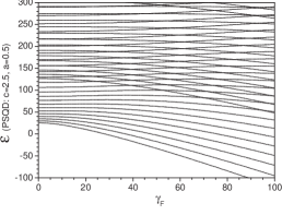
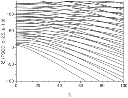
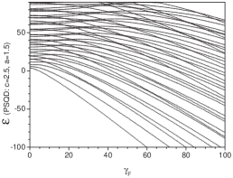
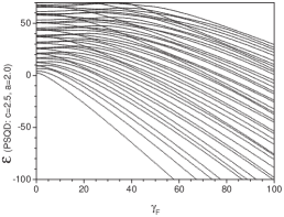
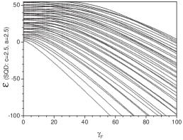
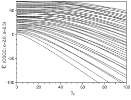
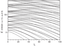
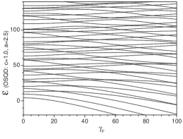
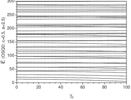
Figure 1: Dependence of eigenenergies ${\cal E}$ (in units of $E_{e}$) of lower part of spectrum of electronic states of QDs at $m=0$ on electric field strength $\gamma_{F}$ (in units of $F_{0}^{*}$): for spherical quantum dot (SQD) with radius $a=c=2.5$, oblate and prolate spheroidal quantum dots (OSQD and PSQD) at different minor semiaxis (for OSQD $c=0.5,1,1.5,2$, $a=2.5$, for PSQD $c=2.5$, $a=0.5,1,1.5,2$).

In Fig. 1 we show the eigenenergies of the lower part of the spectrum ${\cal E}_{t}$, $t=1,...,40$ at $m=0$ for OSQD $(c=0.5,1,1.5,2,a=2.5)$, SQD $(c=2.5,a=2.5)$ and PSQD $(c=2.5,a=0.5,1,1.5,2)$ as functions of the dimensionless strength $\gamma_{F}$ of the electric field. In spite of the fact that at $\gamma_{F}=0$ the eigenfunctions of SQD, OSQD and PSQD have definite z-parity, and, therefore, exhibit additional integrals of motion and separation of variables in spherical and spheroidal coordinates systems, the spectrum of eigenvalues at fixed $m$ is simple, i.e., nondegenerate, similar to the case $\gamma_{F}\neq 0$, when the eigenfunctions have no definite z-parity. At $\gamma_{F}=0$ a one-to-one correspondence rule $n_{\rho p}+1=n_{p}=i=n=n_{r}+1$, $i=1,2,...$ and $n_{zp}=l-|m|$ holds between the quantum numbers $(n,l,m,\hat{\sigma}={(-1)^{|m|}\sigma})$ of SQD with the radius $r_{0}=a=c$, the spheroidal quantum numbers $\{n_{\xi}=n_{r},n_{\eta}=l-|m|,m,\sigma\}$ of PSQD with the major $c$ and the minor $a$ semiaxes, and the adiabatic set of quantum numbers $[n_{p}=n_{\rho p}+1,n_{zp},m,\sigma]$ under the continuous variation of the parameter $\zeta_{ac}=a/c$. At $\gamma_{F}=0$ there is a one-to-one correspondence rule $n_{o}=n_{zo}+1=2n-(1+\sigma)/2$, $n=1,2,3,...$ and $n_{\rho o}=(l-|m|-(1-\sigma)/2)/2$, between the sets of spherical quantum numbers $(n,l,m,\hat{\sigma}={(-1)^{|m|}\sigma})$ of SQD with the radius $r_{0}=a=c$ and spheroidal ones $\{n_{\xi}=n_{r},n_{\eta}=l-|m|,m,\sigma\}$ of OSQD with the major $a$ and the minor $c$ semiaxes, and the adiabatic set of cylindrical quantum numbers $[n_{o}=n_{zo}+1,n_{\rho o},m,\sigma]$ under the continuous variation of the parameter $\zeta_{ca}=c/a$.

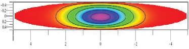
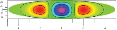
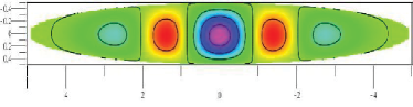
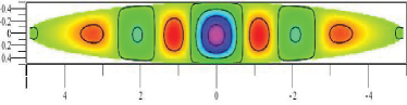
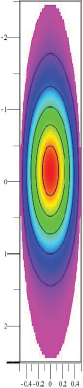
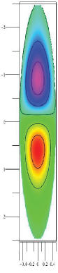
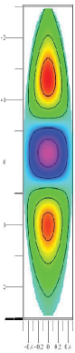
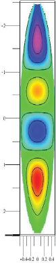
Figure 2: Eigenfunctions of sixth order of PT of 2D BVP for oblate SQD $a=5$, $c=0.5$, $[t=n_{zo}=0$, $n=n_{o}=1,2,3,4$, $m=0$] in electric field $\gamma_{F}=-10$ (weak asymmetry by $z$ - axis i.e. by minor ellipsoid axis).Eigenfunctions of sixth order of PT of 2D BVP for prolate SQD $c=2.5$, $a=0.5$,[$t=n_{\rho p}=0$, $n=n_{p}=0,1,2,3,4$, $m=0$] in electric field $\gamma_{F}=-1$ (asymmetry by $z$ - axis i.e. by major ellipsoid axis).

One can see that when the parameter $\gamma_{F}$ increases the eigenvalues ${\cal E}_{t}$ decrease faster for SQD, slower for PSQD and even more slower for OSQD, because the influence of the electric field for OSQD at $c=0.5$ is essentially weaker than for PSQD at $c=2.5$. With increasing $\gamma_{F}$ a series of exact crossings of eigenenergies with different values of quantum numbers for PSQD and OSQD occur at $\gamma_{F}\gtrsim 20$ and a series of avoided crossings for SQD occur at $\gamma_{F}\gtrsim 10$. With further growth of the parameter they first increase and then begin to decrease. Indeed, with the growth of $\gamma_{F}$ the eigenfunctions with smaller number of nodes in the longitudinal variable $z$ are localized (see Fig.2) in the vicinity of the equilibrium point, and the corresponding eigenenergies decrease. Increasing the number of nodes is accompanied with delocalization of the wave functions, and the corresponding eigenenergies increase and then decrease again. For PSQD the density of states per unit energy for the eigenfunction with the same number of nodes $n_{\rho p}$ in the transverse variable $\rho$ is greater (i.e., the separation between the adjacent energy levels is smaller) than the density of states for the function having the same number of nodes $n_{zp}$ in the longitudinal variable $z$. For this reason in Fig. 1 one can see three crossing series of curves with different number of $\rho$-nodes $n_{\rho p}=0,1,2$, the lower of them (e.g., with $a=0.5$, $n_{\rho p}=0$, and $n_{zp}$ from $0$ to $12$) are decreasing at all $\gamma_{F}\geq 0$, while the upper ones (e.g., with $a=0.5$, $n_{\rho p}=0$, and $n_{zp}$ starting from 13) with the energies, exceeding that of the state ($n_{\rho p}=1$) without $z$-nodes ($n_{zp}=0$), increase from the beginning and then start to decrease. Thus, at small $\gamma_{F}$ the energy levels for the groups of states with even $n_{\rho p}=0,2...$ and odd $n_{\rho p}=1,3...$ number of nodes are repulsing and crossing.

For OSQD, on the contrary, the number of energy levels per unit energy for the eigenfunctions having the same number $n_{\rho o}$ of $\rho$-nodes is smaller (i.e., the separation between the adjacent levels is larger) than that for the eigenfunctions having the same number $n_{zo}$ of $z$-nodes. Therefore, in Fig. 1 one can see four crossing series of almost ’parallel’ curves with different number $n_{zo}=0,1,2,3$ of $z$-nodes.

For OSQD and PSQD the crossings of the energy levels that occur with increasing $\gamma_{F}$ are similar to the exact crossings of the energy levels with decreasing $c$ semiaxis in OSQD and PSQD without electric field ($\gamma_{F}=0$), i.e., we observe the accidental degeneracy, which is known to be generally associated with the existence of an additional integral of motionYaf12 and with the separability of variables in oblate and prolate spheroidal coordinate systems. Thus, from our observations it follows that an additional approximate integral of motion should exist.

For SQD eigenfunction with different numbers of $\rho$- and $z$-nodes, $n_{\rho}$ and $n_{z}$, and with increasing $\gamma_{F}$ the series of crossings become mixed. Note, that the eigenenergies of the states with the same z-parity at $\gamma_{F}=0$ are repulsed with increasing $\gamma_{F}$ (e.g., [$t=9$, $n=1$, $l=5$, ${\cal E}_{9}(\gamma_{F}=0)=14.01$] and [$t=10$, $n=3$, $l=0$, ${\cal E}_{10}(\gamma_{F}=0)=14.21$]), but the states with different z-parity are attracted (e.g., [$t=7$, $n=1$, $l=4$, ${\cal E}_{7}(\gamma_{F}=0)=10.71$] and [$t=8$, $n=2$, $l=2$, ${\cal E}_{8}(\gamma_{F}=0)=13.24$]). This fact should be also associated with the existence of approximate integrals of motion. Indeed, from Fig 1 one can see that for SQD at $a=c=2.5$ with increasing $\gamma_{F}$ the series of exact crossings appear.

III The PTLJ in nondiagonal adiabatic approximation

We expand the potentials (12) and (13) of the BVP (9) and (10) in Taylor series in the vicinity of $x_{s}=0$:

$$E_{i}(x_{s})=E_{i;0}+\sum_{k=1}^{k_{\max}}\frac{E_{i;0}}{\tau^{2k}}x_{s}^{2k},\quad U_{ij}(x_{s})=U_{ij;0}+\sum_{k=1}^{k_{\max}}\frac{\tilde{U}_{ij;k}}{\tau^{2k}}x_{s}^{2k},$$ (14)

$$H_{ij}(x_{s})=\sum_{k=1}^{k_{\max}}k\frac{H_{ij;0}}{\tau^{2k}}x_{s}^{2k},Q_{ij}(x_{s})=\sum_{k=1}^{k_{\max}}\frac{Q_{ij;0}}{\tau^{2k-1}}x_{s}^{2k-1},$$

where $\tilde{U}_{ij;k}=\frac{(2k-3)!!}{(2k)!!}U_{ij;0}$ and the parameter $\tau$ equals $\tau=a$ for OSQD, and $\tau=c$ for PSQD. Substitution of expansions (14) into Eq. (9) leads to the BVP for a set of ODEs of slow subsystem with respect to the unknown vector functions ${\mbox{\boldmath$\chi$}}_{t}(x_{s})=(\chi_{1;t}(x_{s}),...,\chi_{j_{\max;t}}(x_{s}))^{T}$ corresponding to the unknown eigenvalues $2E_{t}\equiv{\cal E}_{t}$:

$$\left(\mathbf{D}^{(0)}+(E_{i;0}-{\cal E}_{t})+\check{V}_{s}(x_{s})+\sum_{k=1}^{k_{\max}}\frac{E_{i;0}+kH_{ii;0}}{\tau^{2k}}x_{s}^{2k}\right)\chi_{i;t}(x_{s})$$ (15)

$$+\sum_{j\neq i}^{j_{\max}}\sum_{k=1}^{k_{\max}}\left(\frac{\tilde{U}_{ij;k}}{\tau^{2k}}x_{s}^{2k}+k\frac{H_{ij;0}}{\tau^{2k}}x_{s}^{2k}+(2k-1)\frac{Q_{ij;0}}{\tau^{2k-1}}x_{s}^{2k-2}+2\frac{Q_{ij;0}}{\tau^{2k-1}}x_{s}^{2k-1}\frac{d}{dx_{s}}\right)\chi_{j;t}(x_{s})=0,$$

where $\tilde{U}_{ij;k}$ is given by the expansion (14) and $\check{V}_{s}(x_{s})=0$ for OSDQ; $U_{ij}(x_{s})=0$ and $\check{V}_{s}(x_{s})={\gamma_{F}}z$ for PSDQ. We choose the unperturbed operator to have the eigenvalues and basis functions of 2D and 1D oscillators. For the OSQD (2D oscillator) with respect to the scaled slow variable $x$ we have: $x_{s}=\rho=\sqrt{x/\sqrt{E_{f}})}$, where $E_{f}=(E_{i^{\prime};0}+H_{i^{\prime}i^{\prime};0})/(4a^{2})={\omega_{i^{\prime}}^{2}/4}$, i.e., the adiabatic frequency, at given $i^{\prime}=n_{o}$

$$L\left(n\right)=\mathbf{D}^{(0)}-E^{(0)},\quad\mathbf{D}^{(0)}=-\left({\frac{d}{dx}x\frac{d}{dx}-\frac{x}{4}-\frac{m^{2}}{4x}}\right),\quad E^{\left(0\right)}\equiv E_{n,m}^{(0)}=n+(|m|+1)/2,$$

$$\Phi_{q}^{{}^{\left(0\right)}}(x)=\frac{\sqrt{q!}x^{|m|/2}\exp(-x/2)L_{q}^{|m|}(x)}{\sqrt{(q+|m|)!}},\quad\int_{0}^{\infty}\Phi_{q}^{{}^{\left(0\right)}}(x)\Phi_{q^{\prime}}^{{}^{\left(0\right)}}(x)dx=\delta_{qq^{\prime}}.$$ (16)

Therefore, the action of the operators $L(n)$ and $x$ on the function $\Phi_{q}^{(0)}(x)\equiv\Phi_{q,m}^{(0)}(x)$ is determined by the recurrence relations stigun

$$L(n)\Phi_{q,m}^{(0)}(x)=(q-n)\Phi_{q,m}^{(0)}(x),$$

$$x\Phi_{q,m}^{(0)}(x)=-\sqrt{q+|m|}\sqrt{q}\Phi_{q-1,m}^{(0)}(x)+$$

$$+(2q+|m|+1)\Phi_{q,m}^{(0)}(x)-\sqrt{q+|m|+1}\sqrt{q+1}\Phi_{q+1,m}^{(0)}(x),$$ (17)

$$x\frac{d\Phi_{q,m}^{(0)}(x)}{dx}=-\sqrt{q+|m|}\sqrt{q}\Phi_{q-1,m}^{(0)}(x)/2$$

$$-\Phi_{q,m}^{(0)}(x)/2+\sqrt{q+|m|+1}\sqrt{q+1}\Phi_{q+1,m}^{(0)}(x)/2.$$

For PSQD (1D oscillator) with respect to the scaled slow variable $x$ $x_{s}=x/\sqrt[4]{E_{f}}$, where $E_{f}=(E_{i^{\prime};0}+H_{i^{\prime}i^{\prime};0})/c^{2}=\omega_{i^{\prime}}^{2}$, i.e., the adiabatic frequency, at given $i^{\prime}=n_{p}$, we have

$$L\left(n\right)=\mathbf{D}^{(0)}-E^{\left(0\right)},\quad\mathbf{D}^{(0)}=-\frac{d^{2}}{dx^{2}}+x^{2},\quad E^{\left(0\right)}\equiv E_{n}^{(0)}=2n+1,\quad n=0,1,....,$$

$$\Phi_{q}^{{}^{\left(0\right)}}(x)=\frac{\exp(-x^{2}/2)H_{q}(x)}{\sqrt[4]{\pi}\sqrt{2^{q}}\sqrt{q!}},\quad\int_{-\infty}^{\infty}\Phi_{q}^{{}^{\left(0\right)}}(x)\Phi_{q^{\prime}}^{{}^{\left(0\right)}}(x)dx=\delta_{qq^{\prime}}.$$ (18)

Correspondingly action of operators $L(n)$, $x$ and $\frac{d}{dx}$ on function$\Phi_{q}^{(0)}(x)$is determined by recurrence relations stigun

$$L(n)\Phi_{q}^{(0)}(x)=2(q-n)\Phi_{q}^{(0)}(x),$$

$$x\Phi_{q}^{(0)}(x)=\frac{\sqrt{q}}{\sqrt{2}}\Phi_{q-1}^{(0)}(x)+\frac{\sqrt{q+1}}{\sqrt{2}}\Phi_{q+1}^{(0)}(x),$$ (19)

$$\frac{d}{dx}\Phi_{q}^{(0)}(x)=\frac{\sqrt{q}}{\sqrt{2}}\Phi_{q-1}^{(0)}(x)-\frac{\sqrt{q+1}}{\sqrt{2}}\Phi_{q+1}^{(0)}(x).$$

The eigenfunctions (15)as functions of the new scaled variable $x$ are sought in the form of expansion over the basis of the normalized functions $\Phi^{(0)}_{q}(x)$, $q=0,1,....$ of the 2D or 1D oscillators with unknown coefficients $b_{j,s}$:

$$\chi_{j;t}(x)=\sum_{q=0}^{q_{\max}}b_{j,q;t}\Phi^{(0)}_{q}(x),\quad b_{j,q<0;t}=b_{j,q>q_{\max};t}=0.$$ (20)

Below we demonstrate that such expansions are appropriate for getting approximate solutions in the lower part of the BVP spectrum (9) and (10). Substitution of the expansion (20) into (15) yields the set of equations

$$\!\!\!\!\!\!\!\!\sum_{q=0}^{q_{\max}}{\hat{\bf A}}_{ii}b_{i,q;t}\Phi^{(0)}_{q}(x)+\sum_{j\neq i=1}^{j_{\max}}\sum_{q=0}^{q_{\max}}{\hat{\bf A}}_{ij}b_{j,q;t}\Phi^{(0)}_{q}(x)=\sum_{q=0}^{q_{\max}}\kappa^{-2}{\cal E}_{t}E_{f}^{-1/2}b_{i,q;t}\Phi^{(0)}_{q}(x),$$ (21)

$$\!\!\!\!\!\!\!\!{\hat{\bf A}}_{ii}=\left(\mathbf{D}^{(0)}+\check{V}_{s}(x)E_{f}^{-3/4}+\kappa^{-2}E_{i;0}E_{f}^{-1/2}+\kappa^{-2}\sum_{k=1}^{k_{\max}}\frac{E_{i;0}+kH_{ii;0}}{{\tau}^{2k}E_{f}^{(k+1)/2}}x^{2k}\right),$$

$$\!\!\!\!\!\!\!\!{\hat{\bf A}}_{ij}=\kappa^{-2}\sum_{k=1}^{k_{\max}}\left(\frac{\tilde{U}_{ij;k}+kH_{ij;0}}{\tau^{2k}E_{f}^{(k+1)/2}}x_{s}^{2k}+\frac{Q_{ij;0}}{{\tau}^{2k-1}E_{f}^{k/2}}\left((2k-1)x^{2k-2}+2x^{2k-1}\frac{d}{dx}\right)\right),$$

where $\kappa=2$ and $\check{V}_{s}(x_{s})=0$ for OSQD; $\kappa=1$ and $\check{V}_{s}(x)={\gamma_{F}}x$ for PSQD. Applying the relations (17) or (19) to get first derivatives of the basis functions, we get the expressions for the action of operators ${\hat{\bf A}}_{ij}$:

$${\hat{\bf A}}_{ij}\Phi^{(0)}_{q}(x)=\sum_{q^{\prime}=0}^{q_{\max}}\alpha_{ij;qq^{\prime}}\Phi^{(0)}_{q^{\prime}}(x)$$ (22)

and, hence, the algebraic eigenvalue problem with respect to the unknown $E_{t}$ and $b_{j,q;t}$

$$\sum_{q=0}^{q_{\max}}\alpha_{ii;q^{\prime}q}b_{i,q;t}+\sum_{j\neq i=1}^{j_{\max}}\sum_{q=0}^{q_{\max}}\alpha_{ij;q^{\prime}q}b_{j,q;t}=\kappa^{-2}{\cal E}_{t}E_{f}^{-1/2}b_{i,q;t}.$$ (23)

In the matrix form it reads as

$$\textbf{AB}_{t}=\kappa^{-2}{\cal E}_{t}E_{f}^{-1/2}\textbf{B}_{t},\quad\textbf{B}_{t^{\prime}}^{T}\textbf{B}_{t}=\delta_{tt^{\prime}},$$

where $\textbf{B}_{t}=(b_{1,0;t},b_{1,1;t},...,b_{1,q_{\max};t},b_{2,0;t},...,b_{j_{\max},q_{\max};t})^{T}$ is a vector with dimension of $j_{\max}(q_{\max}+1)$, and A is a positive defined symmetric matrix having the dimensions $(j_{\max}(q_{\max}+1))\times(j_{\max}(q_{\max}+1))$ with the elements $A_{(q_{\max}+1)(i-1)+q+1,(q_{\max}+1)(j-1)+q^{\prime}+1}=\alpha_{ij;qq^{\prime}}$.

Note, that the approximation with nonzero elements on the diagonal of the matrix $\textbf{A}=\{\alpha_{ii;q^{\prime}q}\}_{q^{\prime},q=0}^{(q_{\max})}\delta_{i=i_{0},j=i_{0}}$, obtained by the action of the diagonal operator ${\hat{\bf A}}_{ii}$, Eq. (21), on the basis function $\Phi^{(0)}_{q}(x)$, Eq.(22), gives the diagonal adiabatic approximation (AA) of PTLJ solution (23), i.e., ${\cal E}_{t}\approx{\cal E}_{i;n},n=0,1,...$ at each fixed $i$. Such adiabatic classification of the eigenenergies is used in Tables discussed below.

Table 3: The convergence of eigenenergies ${\cal E}_{t}$ of Eq. (23) vs order $k_{\max}$ of approximation of effective potentials from (14) for $j_{\max}=4$ and $q_{\max}=60$ basis functions at $\gamma_{F}=0$. Fast and slow variables $x_{f}=z$ and $x_{s}=\rho$ (oblate SQD and spherical QD), number of nodes $i=(n_{zo}=n_{o}-1,n_{\rho o})$.

$k_{\max}$	$a=2.5$, $c=0.5$			$a=2.5$, $c=2.5$
$(n_{zo},n_{\rho o})$	(0,0)	(0,1)	(2,0)	(0,0)	(0,1)	(2,0)
8	12.668 20	19.067 45	96.714 86	1.192 415	2.998 982	5.325 360
12	12.749 67	19.813 83	96.750 70	1.377 572	4.088 539	5.868 629
20	12.784 07	19.838 42	96.751 72	1.132 323	5.084 082	6.735 687
N$(j_{\max}=4)$	12.764 82	20.040 74	96.752 15	1.579 273	5.316 872	6.317 204

Table 4: The convergence of eigenenergies ${\cal E}_{t}$ of Eq. (23) vs order $k_{\max}$ of approximation of effective potentials from (14) for $j_{\max}=4$ and $q_{\max}=60$ basis functions at $\gamma_{F}=0$. Fast and slow variables $x_{f}=\rho$ and $x_{s}=z$ (prolate SQD and spherical QD), number of nodes $i=(n_{\rho p},n_{zp})$.

$k_{\max}$	$c=2.5$, $a=0.5$			$c=2.5$, $a=2.5$
$(n_{\rho p},n_{zp})$	(0,0)	(0,2)	(1,0)	(0,0)	(0,2)	(1,0)
8	25.179 14	34.076 77	126.445 9	1.471 911	4.270 174	5.614 892
12	25.199 62	34.468 84	126.456 0	1.536 121	4.716 984	6.188 144
20	25.201 16	34.522 02	126.456 1	1.563 492	5.182 198	6.266 533
N$(j_{\max}=4)$	25.201 21	34.525 12	126.456 1	1.579 239	5.316 732	6.317 058

The convergence of eigenenergies of Eq. (23) vs the order $k_{\max}$ of approximation of the effective potentials (14) for $j_{\max}=4$ and $q_{\max}=60$ is shown in Tables 3 and 4 for OSDD, PSQD, and SQD at $\gamma_{F}=0$ and in Table 5 at $\gamma_{F}=-10$ for PSQD and SQD. Table 4 shows that for PSQD we have upper estimate and monotonic convergence with increasing $k_{\max}$ to the numerical results at $j_{\max}=4$. Similar behavior is observed for OSQD, however the accuracy of approximation of the effective potentials is worse, especially for the lowest effective potential $i^{\prime}=1$, corresponding to the ground state of the fast subsystem, because the upper estimates are violated. These Tables show also that such expansions have faster convergence for strongly oblate or prolate spheroidal QDs than for spherical ones.

Table 5: The convergence of eigenenergies ${\cal E}_{t}$ of Eq. (23) vs order $k_{\max}$ of approximation of effective potentials from (14) for $j_{\max}=4$ and $q_{\max}=60$ basis functions at $\gamma_{F}=-10$. Fast and slow variables $x_{f}=\rho$ and $x_{s}=z$ (prolate SQD and spherical QD), number of nodes $i=(n_{\rho p},n_{zp})$.

$k_{\max}$	$c=2.5$, $a=0.5$, $\gamma_{F}=-10$			$c=2.5$, $a=2.5$, $\gamma_{F}=-10$
$(n_{\rho p},n_{zp})$	(0,0)	(0,2)	(1,0)	(0,0)	(0,2)	(1,0)
8	20.221 65	30.913 36	125.306 2	-19.673 98	-5.378 707	-1.784 110
12	20.607 33	32.375 40	125.331 6	-15.348 50	-6.881 266	-2.605 091
20	20.658 46	32.674 45	125.332 2	-12.194 45	-2.204 160	-1.336 853
N$(j_{\max}=4)$	20.6620̇3	32.708 77	125.332 2	-10.844 02	-1.511 063	1.129 039

IV PTRS for BVP for OSQD in electric field by fast variables

To have an analytic representation of the matrix elements (11) for small $\gamma_{F}$, one can use $\check{V}_{f}(x_{f};{x_{s}})=2\gamma_{F}z$, ${\check{V}_{fs}(x_{f},{x_{s}})=0}$ as potentials for OSQD instead of the potentials (12) introduced in Section 2.1. Then we arrive at the Sturm-Lioville problem for the OSQD in fast variable expressed in the form

$$\left(-\frac{d^{2}}{dz^{2}}-\epsilon z-E_{j}(\rho)\right)B_{j}(z;\rho)=0,$$ (24)

$$\langle B_{i}(\rho)|B_{j}(\rho)\rangle=\int_{-L(\rho)/2}^{L(\rho)/2}B_{i}(z;\rho)B_{j}(z;\rho)dz=\delta_{ij},$$

where $\epsilon=\gamma_{F}$ is the electric field strength considered here as a formal parameter of the PT, implying a small interval $\rho\in(0,L(\rho)=2c\sqrt{1-\rho^{2}/a^{2}})$ of the scalar product $\langle B_{i}(\rho)|B_{j}(\rho)\rangle$. The solutions $B_{j}^{(0)}(z;\rho)$ and $E_{j}^{(0)}(\rho)$ of the unperturbed equation (at $\epsilon=0$) have the form

$$\{B_{j}^{(0)}(z;\rho),E_{j}^{(0)}(\rho)\}=\left\{\begin{array}[]{ll}\{B_{j}^{s}(z;\rho),E_{j}^{s}(\rho)\},&\mbox{ for even }j=2,4,...;\\ \{B_{j}^{c}(z;\rho),E_{j}^{c}(\rho)\},&\mbox{ for odd }j=1,3,...\end{array}\right\},$$ (27)

where

$$B_{j}^{s}(z;\rho)=\sqrt{2/L(\rho)}\sin(\pi jz/L(\rho)),\quad B_{j}^{c}(z;\rho)=\sqrt{2/L(\rho)}\cos(\pi jz/L(\rho)),$$

$$E_{j}^{s}(\rho)=(\pi j/L(\rho))^{2},\quad E_{j}^{c}(\rho)=(\pi j/L(\rho))^{2}.$$

We seek for the eigenfunctions $B_{j}(z;\rho)$ and the eigenvalues $E_{j}(\rho)$ in the form of power expansions

$$B_{j}(z;\rho)=\sum_{k=0}^{k_{\max}}\epsilon^{k}B_{j}^{(k)}(z;\rho),\quad E_{j}(\rho)=\sum_{k=0}^{k_{\max}}\epsilon^{k}E_{j}^{(k)}(\rho).$$ (28)

Substituting Eq. (28) into Eqs. (24) and equating the coefficients at the same powers of $\epsilon$, we arrive at the system of inhomogeneous differential equations with respect to corrections $E_{j}^{(k)}$ and $B_{j}^{(k)}(z;\rho)$:

$$\!\!\!\!\!\!\!\!\!\!\!\left(-\frac{d^{2}}{dz^{2}}-E_{j}^{(0)}(\rho)\right)B_{j}^{(k)}(z;\rho)=\left(z+E_{j}^{(1)}(\rho)\right)B_{j}^{(k-1)}(z;\rho)+\sum_{p=2}^{k}E_{j}^{(p)}(\rho)B_{j}^{(k-p)}(z;\rho),$$ (29)

$$\sum_{p=0}^{k}\langle B_{j}^{(p)}(\rho)|B_{j}^{(k-p)}(\rho)\rangle=0.$$

In each $k$-th order of the perturbation theory (PT) the solutions becoming zero at the boundary points $(z=\pm L(\rho)/2$ are sought in the form

$$B_{j}^{(k)}(z;\rho)=\left\{\begin{array}[]{ll}\sum\limits_{\nu=0}^{\nu_{\max}}B_{j}^{s}(z;\rho)S^{(k)}_{\nu}z^{\nu}+(z^{2}-(L(\rho)/2)^{2})\sum\limits_{\nu=0}^{\nu_{\max}-2}B_{j}^{c}(z;\rho)C^{(k)}_{\nu+2}z^{\nu},&j=2,4,...\\ \sum\limits_{\nu=0}^{\nu_{\max}}B_{j}^{s}(z;\rho)C^{(k)}_{\nu}z^{\nu}+(z^{2}-(L(\rho)/2)^{2})\sum\limits_{\nu=0}^{\nu_{\max}-2}B_{j}^{c}(z;\rho)S^{(k)}_{\nu+2}z^{\nu},&j=1,3,...\end{array}\right\}.$$ (32)

Substituting Eq. (32) into the corresponding equation (29) of the $k$-th order of the PT, and extracting the coefficients at $B_{j}^{s}(z;\rho)z^{\nu}$ and $B_{j}^{c}(z;\rho)z^{\nu}$, $\nu=0,...,\nu_{\max}$, we arrive at the set of algebraic equations with respect to unknowns $E_{j}^{(k)}(\rho)$, $S^{(k)}_{\nu}$ and ${}^{(k)}_{\nu}$, for even $j$:

$$-(-1)^{j}(\nu+1)(L(\rho)/2)\pi jC^{(k)}_{\nu+3}-(\nu+2)(\nu+1)S^{(k)}_{\nu+2}+(-1)^{j}2(\nu+1)\pi jC^{(k)}_{\nu+1}$$

$$\quad-E_{j}^{(1)}(\rho)S^{(k-1)}_{\nu}-S^{(k-1)}_{\nu-1}-\sum_{p=2}^{k-1}E_{j}^{(p)}(\rho)S^{(k-p)}_{\nu}-E_{j}^{(k)}(\rho)\delta_{\nu,0}=0,$$

$$+(\nu+1)(\nu+2)(L(\rho)/2)^{2}C^{(k)}_{\nu+4}-(\nu+2)(\nu+1)C^{(k)}_{\nu+2}-(-1)^{j}2(\nu+1)\pi jS^{(k)}_{\nu+1}$$

$$\quad-E_{j}^{(1)}(\rho)(C^{(k-1)}_{\nu}-(L(\rho)/2)^{2}C^{(k-1)}_{\nu+2})-C^{(k-1)}_{\nu-1}+(L(\rho)/2)^{2}C^{(k-1)}_{\nu+1})$$

$$\quad-\sum_{p=2}^{k-1}E_{j}^{(p)}(\rho)(C^{(k-p)}_{\nu}-(L(\rho)/2)^{2}C^{(k-p)}_{\nu+2})=0.$$

For odd $j$ the same unknowns are calculated using the equations (IV) (IV) with the replacement $C^{(p)}\leftrightarrows S^{(p)}$. The unknowns ${}^{(k)}_{0}$ for even $j$ and $S^{(k)}_{0}$ for odd $j$ are determined from the respective conditions:

$$\sum_{p=0}^{k}\sum_{\nu,\nu^{\prime}}\left(S^{(p)}_{\nu}S^{(k-p)}_{\nu^{\prime}}\langle B_{j}^{s}(\rho)|z^{\nu+\nu^{\prime}}|B_{j}^{s}(\rho)\rangle\right.$$ (33)

$$\left.+[(C^{(p)}_{\nu}S^{(k-p)}_{\nu^{\prime}}+S^{(p)}_{\nu}C^{(k-p)}_{\nu^{\prime}})+(L(\rho)/2)^{2}(C^{(p)}_{\nu+1}S^{(k-p)}_{\nu^{\prime}+1}+S^{(p)}_{\nu+1}C^{(k-p)}_{\nu^{\prime}+1})]\langle B_{j}^{s}(\rho)|z^{\nu+\nu^{\prime}}|B_{j}^{c}(\rho)\rangle\right.$$

$$\left.+[(C^{(p)}_{\nu}C^{(k-p)}_{\nu^{\prime}})-2(L(\rho)/2)^{2}C^{(p)}_{\nu+1}C^{(k-p)}_{\nu^{\prime}+1}+(L(\rho)/2)^{4}C^{(p)}_{\nu+2}C^{(k-p)}_{\nu^{\prime}+2}]\langle B_{j}^{c}(\rho)|z^{\nu+\nu^{\prime}}|B_{j}^{c}(\rho)\rangle\right),$$

and $S^{(k)}_{0}$ for odd $j$ is calculated from the equation (33) with the replacement $C^{(p)}\leftrightarrows S^{(p)}$. This algorithm was implemented using the Maple environment. The run was performed until the maximal order of the PT $k_{max}=8$. Below we present the first few coefficients of the eigenvalue expansion, truncated by the terms proportional to $\epsilon^{6}=\gamma_{F}^{6}$

$$E_{j}(\rho)=\frac{\pi^{2}j^{2}}{((L(\rho))^{2}}+\frac{((L(\rho))^{4}(\pi^{2}j^{2}-15)}{48\pi^{4}j^{4}}\epsilon^{2}+\frac{(L(\rho))^{10}(1980-210\pi^{2}j^{2}+\pi^{4}j^{4})}{2304\pi^{10}j^{10}}\epsilon^{4},$$ (34)

the eigenfunctions truncated by the terms proportional to $\epsilon^{2}=\gamma_{F}^{2}$

$$B_{j}(z;\rho)=\left\{\begin{array}[]{ll}B_{j}^{s}(z;\rho)+\left(-\frac{(L(\rho))^{2}zB_{j}^{s}(z;\rho)}{4\pi^{2}j^{2}}+\frac{L(\rho)(z^{2}-(L(\rho)/2)^{2})B_{j}^{c}(z;\rho)}{4\pi j}\right)\epsilon,&j=2,4,...\\ B_{j}^{c}(z;\rho)+\left(-\frac{(L(\rho))^{2}zB_{j}^{c}(z;\rho)}{4\pi^{2}j^{2}}-\frac{L(\rho)(z^{2}-(L(\rho)/2)^{2})B_{j}^{s}(z;\rho)}{4\pi j}\right)\epsilon,&j=1,3,...\end{array}\right\},$$

and the diagonal effective potentials, truncated by the terms proportional to $\epsilon^{6}=\gamma_{F}^{6}$

$$H_{jj}(z)=\left(\frac{dL(\rho)}{d\rho}\right)^{2}\left(\frac{\pi^{2}j^{2}+3}{12(L(\rho))^{2}}+\frac{(L(\rho))^{4}(-2880+258\pi^{2}j^{2}+7\pi^{4}j^{4})}{576\pi^{6}j^{6}}\epsilon^{2}\right.$$

$$\left.+\frac{L(\rho)^{10}(3510000-389880\pi^{2}j^{2}+3321\pi^{4}j^{4}+13\pi^{6}j^{6})}{27648\pi^{12}j^{12}}\epsilon^{4}\right).$$ (36)

V The PTRS in the diagonal adiabatic approximation

The desired solutions ofthe original 2D BVP (4) are determined by the diagonal approximation of the Kantorovich expansion(7) at fixed $m$

$$\Psi_{i;n}^{m}(x_{f},x_{s})\approx B_{i}(x_{f};x_{s})\chi_{i;n}(x_{s}).$$

The diagonal approximation of the BVP (9) and (10) in the slow variable has the form

$$\left(-\frac{1}{x_{s}^{d}}\frac{d}{dx_{s}}x_{s}^{d}\frac{d}{dx_{s}}+\frac{\tilde{m}}{x_{s}^{2}}+V_{i}(x_{s})-{\cal E}_{i;n}\right)\chi_{i;n}(x_{s})=0.$$ (37)

and the eigenfunctions satisfy the orthonormalization conditions on the semiaxis $[x_{s}^{\min}=0,{x_{s}^{\max}}=\infty)$ at $d=1$ for the OSQD and on the axis $(x_{s}^{\min}=-\infty,{x_{s}^{\max}}=\infty)$ at $d=0$ for the OSQD

$$\int\nolimits_{x_{s}^{\min}}^{x_{s}^{\max}}\chi_{i;n}(x_{s}))\chi_{i,n^{\prime}}(x_{s})(x_{s})^{d}dx_{s}=\delta_{nn^{\prime}}.$$ (38)

Here $V_{i}(x_{s})=\check{V}_{s}(x_{s})+E_{i}(x_{s})+DH_{ii}(x_{s})$, where the parameter $D$ is $D=0$ for the crude adiabatic approximation and $D=1$ for the adiabatic approximation; $\check{V}_{s}(x_{s})=0$, $E_{i}(x_{s})$ and $H_{ii}(x_{s})$, Eqs. (34)–(36), for OSQD and $\check{V}_{s}(x_{s})=2\gamma_{F}z$, $E_{i}(x_{s})$ and $H_{ii}(x_{s})$, Eq. (13), for PSQD; ${\cal E}_{i;n}$ are the eigenenergies of a lower part of thespectrum ${\cal E}_{i;0}<{\cal E}_{i;1}<...<{\cal E}_{i;n}$ enumerated in the ascending order by the number of nodes $n=0,1,2,...$ of the eigenfunctions $\chi_{i;n}(x_{s})$ at fixed adiabatic quantum numbers $i=n_{o}$ for OSQD and $i=n_{p}$ for PSQD. The potential function $V_{i}(x_{s})$ is expanded in powers of the small parameter $\varepsilon$

$$V_{i}^{[j_{{\max}}]}(x_{s})=V_{i}^{(0)}+\kappa^{-2}\omega_{i}^{2}x_{s}^{2}+\kappa^{-2}\sum_{j=1}\nolimits^{j_{max}}V_{i}^{(j)}(x_{s})\varepsilon^{j}.$$ (39)

For OSQD at the values of the parameters $d=1$, $\varepsilon=c^{-2},\quad\kappa=2,\quad\tilde{m}=m$ the coefficients $V_{i}^{(j)}$ are determined by Taylor expansion of the effective potentials (34), (36) in the vicinity of the equilibrium point $x_{s}=0$. With the accuracy up to order of $O(\gamma_{F}^{6})$ the coefficients $V_{i}^{(j)}$ and $\omega_{i}^{2}$ are expressed as:

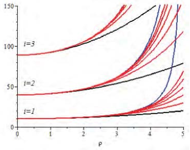
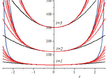
Figure 3: Three potential functions $V_{i}(x_{s})$ for oblate $x_{s}=\rho$ and prolate $x_{s}=z$ spheroids and their power expansions till sixth order with account of adiabatic frequencies $\omega_{i}$ and lower bound shifts $V_{i}^{(0)}$.

$$V_{i}^{(0)}=\frac{\pi^{2}n_{o}^{2}}{4c^{2}}+{\gamma_{F}^{2}}\frac{c^{4}(\pi^{2}n_{o}^{2}-15)}{3\pi^{4}n_{o}^{4}}+{\gamma_{F}^{4}}\frac{4c^{10}(\pi^{4}n_{o}^{4}-210\pi^{2}n_{o}^{2}+1980)}{9\pi^{10}n_{o}^{10}},$$ (40)

$$\omega_{i}^{2}=\frac{\pi^{2}n_{o}^{2}}{(ac)^{2}}+D\frac{3+\pi^{2}n_{o}^{2}}{a^{4}}+\gamma_{F}^{2}\left(-\frac{8c^{4}(\pi^{2}n_{o}^{2}-15)}{3a^{2}\pi^{4}n_{o}^{4}}+D\frac{4c^{6}(7\pi^{4}n_{o}^{4}+258\pi^{2}n_{o}^{2}-2880)}{9a^{4}\pi^{6}n_{o}^{6}}\right)$$

$$+\gamma_{F}^{4}\left(-\frac{80c^{10}(\pi^{4}n_{o}^{4}-210\pi^{2}n_{o}^{2}+1980)}{9a^{2}\pi^{10}n_{o}^{10}}+D\frac{16c^{12}(13\pi^{6}n_{o}^{6}+3321\pi^{4}n_{o}^{4}-389880\pi^{2}n_{o}^{2}-3510000)}{27a^{4}\pi^{12}n_{o}^{12}}\right),$$

$$V_{i}^{(j)}=\left(\frac{\pi^{2}n_{o}^{2}}{(ac)^{2}}+jD\frac{3+\pi^{2}n_{o}^{2}}{a^{4}}+\gamma_{F}^{2}\left(-\frac{4c^{4}(\pi^{2}n_{o}^{2}-15)}{3a^{4}\pi^{4}n_{o}^{4}}\delta_{i2}-D\frac{4c^{6}(7\pi^{4}n_{o}^{4}+258\pi^{2}n_{o}^{2}-2880)}{9a^{6}\pi^{6}n_{o}^{6}}\delta_{i2}\right)\right.$$

$$\left.+\gamma_{F}^{4}\left(\frac{16c^{10}(\pi^{4}n_{o}^{4}-210\pi^{2}n_{o}^{2}+1980)}{9a^{4}\pi^{10}n_{o}^{10}}(10\delta_{i2}-10\frac{\delta_{i3}}{a^{2}}+5\frac{\delta_{i4}}{a^{4}}-\frac{\delta_{i5}}{a^{6}})\right.\right.$$

$$\left.\left.+D\frac{16c^{12}(13\pi^{6}n_{o}^{6}+3321\pi^{4}n_{o}^{4}-389880\pi^{2}n_{o}^{2}-3510000)}{27a^{6}\pi^{12}n_{o}^{12}}(-4\delta_{i2}+6\frac{\delta_{i3}}{a^{2}}-4\frac{\delta_{i4}}{a^{4}}+\frac{\delta_{i5}}{a^{6}})\right)\right)x_{s}^{2j+2}.$$

For PSQD at the values of the parameters $d=0$, $\varepsilon=1$, $\kappa=1$, $\tilde{m}=0$ the coefficients $V_{i}^{(j)}$ are sought in the form of a Taylor expansion in powers of $\bar{x}_{s}=(x_{s}-x_{0})$ and $\gamma_{F}$ of the effective potentials $V_{i}(x_{s},\gamma_{F})=E_{j}(x_{s})+DH_{jj}(x_{s})+\gamma_{F}x_{s}$, Eq. (13). The expansion coefficients $x_{0}=\sum_{k}\tau_{2k+1}\gamma_{F}^{2k+1}$ are sought from the equilibrium condition $\left.\frac{\partial V_{i}(x_{s},\gamma_{F})}{\partial x_{s}}\right|_{x_{s}=x_{0}}=0$ at fixed $\gamma_{F}$. With the accuracy up to $O(\gamma_{F}^{5})$ the coefficients $V_{i}^{(j)}$ and $\omega_{i}^{2}$ are expressed as:

$$V_{i}^{(0)}=-2\tau_{1}\gamma_{F}^{2}-2\tau_{3}\gamma_{F}^{4}+\alpha_{n_{p},|m|}^{2}/(a^{2})+D(1+\alpha_{n_{p},|m|}^{2})/(3c^{4})$$

$$+\gamma_{F}^{2}\tau_{1}^{2}(\alpha_{n_{p},|m|}^{2}/(a^{2}c^{2})+D(1+\alpha_{n_{p},|m|}^{2})2/(3c^{4}))$$

$$+\gamma_{F}^{4}\tau_{1}(\alpha_{n_{p},|m|}^{2}(\tau_{1}^{3}+2c^{2}\tau_{3})/(a^{2}c^{4})+2D(1+\alpha_{n_{p},|m|}^{2})(\tau_{1}^{3}+\tau_{3}c^{2})/(3c^{6}),$$

$$\omega_{i}^{2}=\left(\alpha_{n_{p},|m|}^{2}/(a^{2}c^{2})+D(1+\alpha_{n_{p},|m|}^{2})/(3c^{4})\right.$$ (41)

$$\left.+\gamma_{F}^{2}\tau_{1}^{2}6(\alpha_{n_{p},|m|}^{2}/(a^{2}c^{4})+D(1+\alpha_{n_{p},|m|}^{2})2/(3c^{6}))\right.$$

$$\left.+\gamma_{F}^{4}\tau_{1}(\alpha_{n_{p},|m|}^{2}(15\tau_{1}^{3}+12c^{2}\tau_{3})/(a^{2}c^{6})+D(1+\alpha_{n_{p},|m|}^{2})(15\tau_{1}^{3}+8\tau_{3}c^{2})/(c^{8})\right),$$

$$V_{i}^{(j)}=\left(+2\gamma_{F}\tau_{1}((i+1)\alpha_{n_{p},|m|}^{2}/(a^{2}c^{2i+2})+D(i+1)^{2}(1+\alpha_{n_{p},|m|}^{2})/(3c^{2i+4}))\right.$$

$$\left.+2\gamma_{F}^{3}(i+1)(\alpha_{n_{p},|m|}^{2}((2i^{2}+7i+6)\tau_{1}^{3}+3\tau_{3}c^{2})/(3a^{2}c^{2i+4})\right.$$

$$\left.\qquad+D(1+\alpha_{n_{p},|m|}^{2})((2i^{3}\tau_{1}^{3}+11i^{2}+20i+12)\tau_{1}^{3}+3(i+1)\tau_{3}c^{2})/(9c^{2i+6})\right)\bar{x}_{s}^{2i+1}$$

$$+\left(\alpha_{n_{p},|m|}^{2}/(a^{2}c^{2i+2})+D(1+\alpha_{n_{p},|m|}^{2})(i+1)/(3c^{2i+4})\right.$$

$$\left.+\gamma_{F}^{2}\tau_{1}^{2}(i+2)(2i+3)(\alpha_{n_{p},|m|}^{2}\/(a^{2}c^{2i+4})+D(1+\alpha_{n_{p},|m|}^{2})(i+2)/(3c^{2i+6}))\right.$$

$$\left.+\gamma_{F}^{4}\tau_{1}(i+2)(2i+3)(\alpha_{n_{p},|m|}^{2}((2i^{2}+11i+15)\tau_{1}^{3}+12c^{2}\tau_{3})/(6a^{2}c^{2i+6})\right.$$

$$\left.\qquad+D(1+\alpha_{n_{p},|m|}^{2})((2i^{3}+17i^{2}+48i+45)\tau_{1}^{3}+12(i+2)\tau_{3}c^{2})/(18c^{2i+8})\right)\bar{x}_{s}^{2i+2},$$

where $\tau_{2k+1}$ is determined from the condition that the coefficient at $\bar{x}_{s}$ is zero:

$$\tau_{1}=\frac{3a^{2}c^{4}}{3c^{2}\alpha_{n_{p},|m|}^{2}+Da^{2}(1+\alpha_{n_{p},|m|}^{2})},\quad\tau_{3}=-\frac{54a^{6}c^{10}(3c^{2}\alpha_{n_{p},|m|}^{2}+2Da^{2}(1+\alpha_{n_{p},|m|}^{2}))}{(3c^{2}\alpha_{n_{p},|m|}^{2}+Da^{2}(1+\alpha_{n_{p},|m|}^{2}))^{4}}.$$

In Fig 3 we show three potential functions $V_{i}(x_{s})$ for oblate $x_{s}=\rho$ and prolate $x_{s}=z$ spheroids and the convergence of the corresponding power expansions till the sixth order with account of adiabatic frequencies $\omega_{i}$ and lower bound shifts $V_{i}^{(0)}$.

We choose the unperturbed operators of Eq. (37) at $\varepsilon=0$ in the expansion (39) in the form (16)–(19) with the eigenvalues and the basis functions of 2D- and 1D- oscillators given in Section 3 with respect to the scaled coordinate $x$, $x_{s}=\sqrt{2x/\omega_{i}}$ and $\bar{x}_{s}=x/\sqrt{\omega}_{i}$, where the adiabatic frequencies $\omega_{i}$ are defined by Eqs. (40) and (41) (at fixed $i^{\prime}=n+1$), respectively. According to (39), we seek for the eigenfunctions $\chi_{i;n}(x_{s})$ and the eigenvalues ${\cal E}_{i;n}$ in the form of expansions in powers of $\varepsilon$ with unknowns $\Phi_{n}^{(k)}$ and $E^{(k)}_{n}$, omitting the notation $m$ for brevity:

$$\chi_{i;n}(x_{s})=\Phi_{n}^{(0)}+\sum_{k=1}^{k_{\max}}\Phi_{n}^{(k)}(x_{s})\varepsilon^{k},\quad$$ (42)

$${\cal E}_{i;n}=V_{i}^{(0)}+\sum_{k=0}^{k_{\max}}{\cal E}_{i;n}^{(k)}=V_{i}^{(0)}+\kappa\omega_{i}\left(E_{i}^{(0)}+\sum_{k=1}^{k_{\max}}E_{n}^{(k)}\varepsilon^{k}\right).$$ (43)

Substituting the expansions (39), (42) and (43) into Eq. (37) and equating the terms with the same power of the parameter $\varepsilon$, we arrive at the recurrence set of inhomogeneous equations of the PT with respect to the unknowns $E^{(k)}_{n}$ and $\Phi^{(p)}_{n}(x)$:

$$L(n)\Phi^{(0)}_{n}(x) = 0\equiv f^{(0)}(x),$$ (44)

$$L(n)\Phi^{(k)}_{n}(x) = \sum_{p=0}^{k-1}(E^{(k-p)}_{n}-V^{(k-p)}_{i})\Phi^{(p)}_{n}(x)\equiv f^{(k)}(x),\quad k\geq 1.$$

with the initial conditions (16) and (18) for OSQD and PSQD, respectively. The solution of this problem is implemented in four steps.

Applying the relations (17) and (19), we expand the right-hand side $f^{(k)}(x)$ and the solutions $\Phi^{(k)}(x)$ of Eqs. (44) over the basis of normalized states $\Phi_{n+s}^{(0)}(x)$, Eqs. (16) and (18):

$$\Phi_{n}^{(k)}(x)=\sum_{s=-{s_{max}}}^{s_{max}}b_{s}^{(k)}\Phi_{n+s}^{(0)}(x),\quad f^{(k)}(x)=\sum_{s=-{s_{max}}}^{s_{max}}f_{s}^{(k)}\Phi_{n+s}^{(0)}(x).$$ (45)

Then a recurrent set of linear algebraic equations for unknown coefficients $b_{s}^{(k)}$ and corrections $E^{(k)}$ is obtained

$$s^{\prime}b^{(k)}_{s}-f^{(k)}_{s}=0,\quad s=-{s_{max}},\ldots,{s_{max}},$$ (46)

where $s^{\prime}=s$ for OSQD and $s^{\prime}=2s$ for PSQD. These equations are solved sequentially for $k=1,2,\ldots,k_{\max}$:

$$f^{(k)}_{0}=0\quad\to E^{(k)};\quad b^{(k)}_{s}=f^{(k)}_{s}/s^{\prime},\quad s=-{s_{max}},\ldots,{s_{max}},\quad s\neq 0.$$ (47)

The initial conditions for this procedure are

$$b^{(0)}_{s}=\delta_{s0},\quad E^{\left(0\right)}=(n+(|\tilde{m}|+1)/2)\quad\mbox{or}\quad E^{\left(0\right)}=(n+1)/2).$$

To obtain the normalized wave function $\Phi_{j}(x)$ up to the $k$-th order, the coefficients $b^{(k)}_{0}$ are determined by the following relation:

$$b_{0}^{(k)}=-\frac{1}{2\langle 0|0\rangle}\sum_{p=1}^{k-1}\sum_{s^{\prime}=-{s_{max}}}^{{s_{max}}}\sum_{s=-{s_{max}}}^{{s_{max}}}b^{(k-p)}_{s}\langle s|s^{\prime}\rangle b^{(p)}_{s^{\prime}}.$$ (48)

The above scheme implemented in Maple was applied to the evaluations of solutions in the analytical form up to the order $k_{\max}=6$ of the PTRS. The first four nonzero coefficients for the energy (43) in the analytic form, truncated by the terms proportional to the sixth power of the electric field strength, $\gamma_{F}^{6}$, in the crude adiabatic approximation (CAA) take the form:

1) For OSQD in terms of minor $c$ and major $a$ semiaxes; the set of adiabatic quantum numbers $[m,n_{o}=n_{zo}+1,n_{\rho o}]$

$$\!\!\!\!\!\!\!\!\!\!\!\!\!\!\!\!V^{(0)}_{n_{o}}=\frac{\pi^{2}n_{o}^{2}}{4c^{2}}+{\gamma_{F}^{2}}\frac{c^{4}(\pi^{2}n_{o}^{2}-15)}{3\pi^{4}n_{o}^{4}}+{\gamma_{F}^{4}}\frac{4c^{10}(\pi^{4}n_{o}^{4}-210\pi^{2}n_{o}^{2}+1980)}{9\pi^{10}n_{o}^{10}},$$ (49)

$$\!\!\!\!\!\!\!\!\!\!\!\!\!\!\!\!{\cal E}^{(0)}_{n_{o};n_{\rho o}}=\left[\frac{\pi n_{o}}{ac}-{\gamma_{F}^{2}}\frac{4c^{5}(\pi^{2}n_{o}^{2}-15)}{3a\pi^{5}n_{o}^{5}}-{\gamma_{F}^{4}}\frac{8c^{11}(2\pi^{4}n_{o}^{4}-360\pi^{2}n_{o}^{2}+3375)}{3a\pi^{11}n_{o}^{11}}\right](2n_{\rho o}+|m|+1),$$

$$\!\!\!\!\!\!\!\!\!\!\!\!\!\!\!\!{\cal E}^{(1)}_{n_{o};n_{\rho o}}=\left[\frac{1}{a^{2}}+{\gamma_{F}^{2}}\frac{4c^{6}(\pi^{2}n_{o}^{2}-15)}{\pi^{6}n_{o}^{6}a^{2}}+{\gamma_{F}^{4}}\frac{16c^{12}(7\pi^{4}n_{o}^{4}-1110\pi^{2}n_{o}^{2}+10350)}{3\pi^{12}n_{o}^{12}a^{2}}\right]\times$$

$$\times(2+6n_{\rho o}+3|m|+6n_{\rho o}^{2}+|m|^{2}+6n_{\rho o}|m|),$$

$$\!\!\!\!\!\!\!\!\!\!\!\!\!\!\!\!{\cal E}^{(2)}_{n_{o};n_{\rho o}}=(2n_{\rho o}+|m|+1)\left[\frac{3c}{2\pi a^{3}n_{o}}(2+2n_{\rho o}+|m|+2n_{\rho o}^{2}+2n_{\rho o}|m|)\right.$$

$$\left.-{\gamma_{F}^{2}}\frac{2c^{7}(\pi^{2}n_{o}^{2}-15)}{3\pi^{7}n_{o}^{7}a^{3}}(54+118n_{\rho o}+16|m|^{2}+59|m|+118n_{\rho o}^{2}+118n_{\rho o}|m|)\right.$$

$$\left.-{\gamma_{F}^{4}}\left(\frac{4c^{13}(1874\pi^{4}n_{o}^{4}-273120\pi^{2}n_{o}^{2}+2536425)}{9\pi^{13}n_{o}^{13}a^{3}}(2n_{\rho o}+|m|+2n_{\rho o}^{2}+2n_{\rho o}|m|)\right.\right.$$

$$\left.\left.+\frac{224c^{13}(8\pi^{4}n_{o}^{4}-1140\pi^{2}n_{o}^{2}+10575)}{9\pi^{13}n_{o}^{13}a^{3}}|m|^{2}+\frac{8c^{13}(326\pi^{4}n_{o}^{4}-48480\pi^{2}n_{o}^{2}+450675)}{3\pi^{13}n_{o}^{13}a^{3}}\right)\right],$$

2) For PSQD in terms of minor $a$ and major $c$ semiaxes, the set of adiabatic quantum numbers $[m,n_{p}=n_{\rho p}+1,n_{zp}]$ and positive zeros $\alpha_{n_{p},|m|}$ of the Bessel functions of the first kind stigun

$$\!\!\!\!\!\!\!\!\!\!\!\!\!\!\!\!V^{(0)}_{n_{p};n_{zp}}=\frac{\alpha_{n_{p},|m|}^{2}}{a^{2}}-{\gamma_{F}^{2}}\frac{a^{2}c^{2}}{4\alpha_{n_{p},|m|}^{2}}+{\gamma_{F}^{4}}\frac{a^{6}c^{4}}{16\alpha_{n_{p},|m|}^{6}},$$ (50)

$$\!\!\!\!\!\!\!\!\!\!\!\!\!\!\!\!{\cal E}^{(0)}_{n_{p};n_{zp}}=\left[\frac{\alpha_{n_{p},|m|}}{ac}+{\gamma_{F}^{2}}\frac{3a^{3}c}{4\alpha_{n_{p},|m|}^{3}}-{\gamma_{F}^{4}}\frac{9a^{7}c^{3}}{16\alpha_{n_{p},|m|}^{7}}\right](2n_{zp}+1),$$

$$\!\!\!\!\!\!\!\!\!\!\!\!\!\!\!\!{\cal E}^{(1)}_{n_{p};n_{zp}}=\left[\frac{3}{4c^{2}}+{\gamma_{F}^{2}}\frac{27a^{4}}{16\alpha_{n_{p},|m|}^{4}}-{\gamma_{F}^{4}}\frac{105a^{8}c^{2}}{64\alpha_{n_{p},|m|}^{8}}\right](2n_{zp}^{2}+2n_{zp}+1),$$

$$\!\!\!\!\!\!\!\!\!\!\!\!\!\!\!\!{\cal E}^{(2)}_{n_{p};n_{zp}}=\frac{3a}{16c^{3}\alpha_{n_{p},|m|}}(2n_{zp}+1)(n_{zp}^{2}+n_{zp}+3)$$

$$+\gamma_{F}^{2}\left(\frac{5a^{5}}{64c\alpha_{n_{p},|m|}^{5}}(2n_{zp}+1)(25n_{zp}^{2}+25n_{zp}+51)-\frac{a^{4}}{4\alpha_{n_{p},|m|}^{4}}(30n_{zp}^{2}+30n_{zp}+11)\right)$$

$$-\gamma_{F}^{4}\left(\frac{45a^{9}c}{256\alpha_{n_{p},|m|}^{9}}(2n_{zp}+1)(23n_{zp}^{2}+23n_{zp}+37)-\frac{3a^{8}c^{2}}{8\alpha_{n_{p},|m|}^{8}}(30n_{zp}^{2}+30n_{zp}+11)\right).$$

Table 6: Convergence of eigenvalues ${\cal E}^{(k_{max})}_{n_{zo},n_{\rho o}}=V^{(0)}_{n_{zo}}+\sum_{k=0}^{k_{max}}{\cal E}^{(k)}_{n_{zo},n_{\rho o}}$ for oblate spheroid $c=0.5$, $a=5$ vs PT order $k_{\max}$ at $\gamma_{F}=0$ . First line ^∗ notes adiabatic shift $V^{(0)}_{n_{zo},n_{\rho o}}$. Last line are results of numerical calculations (Num).

$k_{\max}$	$n_{zo}=0$,$n_{\rho o}=0$	$n_{zo}=0$,$n_{\rho o}=1$	$n_{zo}=0$,$n_{\rho o}=2$	$n_{zo}=0$,$n_{\rho o}=3$	$n_{zo}=0$,$n_{\rho o}=4$
*	11.12624146	13.63951558	16.15278970	18.66606383	21.17933795
0	11.20624146	14.19951558	17.67278970	21.62606383	26.05933795
1	11.21006118	14.23389305	17.80647986	21.97365822	26.78126477
2	11.21026382	14.23433886	17.80254859	21.95100281	26.71094787
3	11.21028027	14.23441723	17.80242765	21.94908610	26.70256215
4	11.21028227	14.23443790	17.80265195	21.95065251	26.70959163
5	11.21028259	14.23444049	17.80264785	21.95052291	26.70875037
Num	11.21028268	14.23444147	17.80265065	21.95050805	26.70857727
$k_{\max}$	$n_{zo}=2$,$n_{\rho o}=0$	$n_{zo}=2$,$n_{\rho o}=1$	$n_{zo}=2$,$n_{\rho o}=2$	$n_{zo}=2$,$n_{\rho o}=3$	$n_{zo}=2$,$n_{\rho o}=4$
*	92.59635079	100.1361731	107.6759955	115.2158178	122.7556402
0	92.67635079	100.6961731	109.1959955	118.1758178	127.6356402
1	92.67762403	100.7076323	109.2405589	118.2916826	127.8762825
2	92.67764654	100.7076818	109.2401221	118.2891654	127.8684695
3	92.67764715	100.7076847	109.2401176	118.2890944	127.8681589
4	92.67764718	100.7076850	109.2401203	118.2891137	127.8682457
5	92.67764718	100.7076850	109.2401203	118.2891132	127.8682422
Num	92.67764718	100.7076850	109.2401204	118.2891132	127.8682419

Table 7: Convergence of eigenvalues ${\cal E}^{(k_{max})}_{n_{\rho_{p}},n_{zp}}=V^{(0)}_{n_{\rho_{p}}}+\sum_{k=0}^{k_{max}}{\cal E}^{(k)}_{n_{\rho_{p}},n_{zp}}$ for prolate spheroid $c=2.5$, $a=0.5$ vs PT order $k_{\max}$ at $\gamma_{F}=0$ . First line ^∗ notes adiabatic shift $V^{(0)}_{n_{\rho_{p}},n_{zp}}$. Last line are results of numerical calculations (Num).

$k_{\max}$	$n_{\rho p}=0$,$n_{zp}=0$	$n_{\rho p}=0$,$n_{zp}=2$	$n_{\rho p}=0$,$n_{zp}=4$	$n_{\rho p}=0$,$n_{zp}=6$	$n_{\rho p}=0$,$n_{zp}=8$
*	25.05660430	32.75204608	40.44748787	48.14292965	55.83837144
0	25.17660430	34.31204608	45.36748787	58.34292965	73.23837144
1	25.18408925	34.42432034	45.88394944	59.80249498	76.41947535
2	25.18465987	34.42810718	45.87103269	59.69485535	76.04779441
3	25.18472054	34.42867746	45.87114189	59.68460238	75.99436976
4	25.18472960	34.42880826	45.87257549	59.69618640	76.05191800
5	25.18473139	34.42883580	45.87259458	59.69511288	76.04351256
Num	25.18472985	34.42884694	45.87265876	59.69512314	76.04210082
$k_{\max}$	$n_{\rho p}=1$,$n_{zp}=0$	$n_{\rho p}=1$,$n_{zp}=2$	$n_{\rho p}=1$,$n_{zp}=4$	$n_{\rho p}=1$,$n_{zp}=6$	$n_{\rho p}=1$,$n_{zp}=8$
*	126.3011119	143.9653618	161.6296118	179.2938617	196.9581117
0	126.4211119	145.5253618	166.5496118	189.4938617	214.3581117
1	126.4243727	145.5742742	166.7746086	19 0.1297223	215.7439616
2	126.4244810	145.5749929	166.7721571	190.1092932	215.6734198
3	126.4244860	145.5750400	166.7721661	190.1084455	215.6690025
4	126.4244863	145.5750447	166.7722178	190.1088627	215.6710754
5	126.4244864	145.5750452	166.7722181	190.1088459	215.6709435
Num	126.4244896	145.5750487	166.7722220	190.1088484	215.6709278

In Tables 6 and 7 we demonstrate how the approximate eigenvalues in the lower part of spectrum for OSQD and PSQD at $m=0$ and $\gamma_{F}=0$ converge to the values calculated numerically with required accuracy in the crude adiabatic approximation with increasing of the PT order $k$. The accuracy was from 8 to 5 digits at $n_{zo}=0$, from 10 to 8 digits at $n_{zo}=2$, from 6 to 4 digits at $n_{\rho p}=0$, and from 8 to 7 digits at $n_{\rho p}=1$, respectively. Note, that the difference between the adiabatic shift $V_{i}^{(0)}$ and the eigenvalues ${\cal E}_{i;n}=V^{(0)}_{i}+{\cal E}^{(0)}_{i;n}$ in the zero order $k=0$ of the PT is small, but increases with growing $n_{\rho o}$ and $n_{zp}$ for OSQD and PSQD, respectively. The shifts $V_{i}^{(0)}$ give the main contribution and provide the lower adiabatic estimate of each set of eigenvalues, generated by the perturbed harmonic oscillator terms with adiabatic frequency $\omega_{i}$. From Tables 6 and 7 one can see that with increasing quantum numbers $n_{zo}$ (or $n_{\rho p}$), related to the fast variable, the accuracy of approximation of the lower part of the spectrum is increasing. This is because the accuracy of the Taylor approximations of potential function (39) in Eq. (37) is improved with increasing the number $i=n_{zo}+1>2$ (or $i=n_{\rho p}+1>2$), which is demonstrated in Fig. 3.

Figure 4: Dependence of eigenenergies ${\cal E}$ (in units of $E_{e}$) of lower part of spectrum of electronic states of OSQDs ($a=2.5$, $c=0.5$) at $m=0$ on electric field strength $\gamma_{F}$ (in units of $F_{0}^{*}$): Solid and dashed lines are eigenenergies calculated by PTRS till 5 order in crude adiabatic approximation: seven solid lines ($n_{zo}=0$, $n_{\rho o}=0,1,...,6$) and four dashed lines ($n_{zo}=1$, $n_{\rho o}=0,1,2,3$) are shown on left panel in interval $\gamma_{F}\in(0,1)$; the first three of solid lines ($n_{zo}=1$, $n_{\rho o}=0,1,2$) and the first two of dashed lines ($n_{zo}=1$ , $n_{\rho o}=0,1$) are shown on lower-right and upper-right panel, respectively, in bigger intervals $\gamma_{F}\in(0,20)$ and $\gamma_{F}\in(0,10)$. Numerical solutions of Eqs. (4) at $j_{\max}=4$ are shown by points.

Figure 5: Dependence of eigenenergies ${\cal E}$ (in units of $E_{e}$) of lower part of spectrum of electronic states of PSQDs ($a=0.5$, $c=2.5$) at $m=0$ on electric field strength $\gamma_{F}$ (in units of $F_{0}^{*}$): Solid and dashed lines are eigenenergies calculated by PTRS till 5 order in crude adiabatic approximation: fifteen solid lines ($n_{\rho p}=0$, $n_{zp}=0,1,...,14$) and three dashed lines ($n_{\rho p}=1$ , $n_{zp}=0,1,2$) are shown on left panel in interval $\gamma_{F}\in(0,0.1)$; the first six of solid lines ($n_{\rho p}=0$, $n_{zp}=0,1,...,5$) are shown on lower-right panel and the dashed lines ($n_{\rho p}=1$ , $n_{zp}=0,1,2$) are shown on upper-right panel in bigger interval $\gamma_{F}\in(0,3)$. Numerical solutions of Eqs. (4) at $j_{\max}=4$ are shown by points.

In Figs. 4 and 5 we show the eigenvalues ${\cal E}$ of the lower part of the spectrum of oblate and prolate QDs versus the electric field strength within small (left panels) and large (right panels) intervals of $\gamma_{F}$, calculated in the crude adiabatic approximation (solid and dashed lines) to compare them with the numerical results (dotted lines). One can see that the eigenvalues calculated using the PT (solid and dashed lines), corresponding to the eigenfunctions with smaller number of nodes along the electric field (i.e., with smaller $n_{zo}$ for OSQD and $n_{zp}$ for PSQD) and with greater number of nodes across the electric field (i.e., with greater $n_{\rho o}$ for OSQD and $n_{\rho p}$ for PSQD), provide better approximation of the eigenvalues, calculated numerically with required accuracy (dotted lines). This property follows from the fact that such functions have better localization in the vicinity of the plane, passing through the QD center transverse to the electric field, i.e., in the region with minimal contribution of the electric field potential to the Hamiltonian of the system. As shown in the right panels of Figs. 4 and 5, the differences between the egienvalues, calculated using the PT and the numerical method, increase faster in a smaller interval of $\gamma_{F}$ for larger PSQD than for smaller OSQD, the size being measured along the direction of the electric field.

The range of the parameter values, for which the PT algorithms are valid, was estimated by means of numerical calculations using the KANTBP program Yu3 , as well as the condition that the mean value of the slow variable is smaller than the size of the major axis of OSQD or PSQD, i.e., $\rho\leq a$ or $z\leq c$, or known estimates of the distribution of nodes of Laguerre or Hermite polynomials stigun . To calculate also the approximate eigenfunctions of the lower part of the spectrum $n=0,...,n_{\max}$ with required numbers $n$ of nodes in the interval $\rho\in(0,a)$ (or $z\in(-c,c)$) for OSQD (or PSQD), one should choose such value of parameter $a=\sqrt{2x_{0}/\omega_{i}}$ (or $c=x_{0}/\sqrt{\omega_{i}}$), that outside this interval $x\in(x_{0}=4n+2|m|+2,\infty)$ (or $|x|\in(x_{0}=(2n+1)^{1/2},\infty)$) the Laguerre (or Hermite) polynomials have no nodes. As an example, in Fig. 2 we show contour plots in zx and xz plane of the first four eigenfunctions of OSQD and PSQD, respectively, that have a required number of nodes (crossings of the function plot with zero plane) in the interval $\rho\in(0,a)$ and $z\in(-c,c)$ at the values $c=0.5$, $a=5$, $c=2.5$, $a=0.5$. One can see that the asymmetry with respect to z-axis of the eigenfunctions of PSQD is greater than that of OSQD, because the variation of well depth of PSQD is greater than of OSQD.

VI Absorption coefficient for an ensemble of QDs

One can use the differences in the energy spectra to verify the considered models of QDs by calculating the absorption coefficient $K(\tilde{\omega}^{ph},\tilde{a},\tilde{c},)$ of an ensemble of identical semiconductor QDs Efros1982 . Since we do not discuss exciton effects in the present paper, the absorption coefficient may be approximately expressed as

$$\tilde{K}(\tilde{\omega}^{ph},\tilde{a},\tilde{c},u)=\sum_{\nu,\nu^{\prime}}\tilde{K}_{\nu,\nu^{\prime}}(\tilde{\omega}^{ph},\tilde{a},\tilde{c},u)=\tilde{A}\sum_{\nu,\nu^{\prime}}\tilde{I}_{\nu,\nu^{\prime}}(u)\delta(\hbar\tilde{\omega}^{ph}-\tilde{W}_{\nu\nu^{\prime}}),$$ (51)

$$\tilde{I}_{\nu,\nu^{\prime}}(u)=\left|\int\tilde{\Psi}^{e}_{\nu}(\tilde{\bf r};\tilde{a},\tilde{c},F,\mu_{e})\tilde{\Psi}^{h}_{\nu^{\prime}}(\tilde{\bf r};\tilde{a},\tilde{c},F,\mu_{h})d^{3}\tilde{\bf r}\right|^{2},\,\,\,\,$$

where $\tilde{A}$ is proportional to the square of the matrix element in the Bloch decomposition, $\tilde{\Psi}^{e}_{\nu}(u)$ and $\tilde{\Psi}^{h}_{\nu^{\prime}}$ are the eigenfunctions of the electron ($e$) and the heavy hole ($h$), $\tilde{E}^{e}_{\nu}$ and $\tilde{E}^{h}_{\nu^{\prime}}$ are the energy eigenvalues for the electron ($e$) and the heavy hole ($h$), depending on the semiaxis size $\tilde{c},\tilde{a}$ for OSQD (or $\tilde{a},\tilde{c}$ for PSQD) and the adiabatic set of quantum numbers $\nu=[n_{zo},n_{\rho o},m]$ and $\nu^{\prime}=[n_{zo}^{\prime},n_{\rho o^{\prime}},m^{\prime}]$ ($\nu=[n_{\rho p},n_{zp},m]$ and $\nu^{\prime}=[n_{\rho p}^{\prime},n_{zp}^{\prime},m^{\prime}]$), where $m^{\prime}=-m$, $\tilde{E}_{g}$ is the band gap width in the bulk semiconductor, $\tilde{\omega}^{ph}$ is the incident light frequency, $\tilde{W}_{\nu\nu^{\prime}}=\tilde{E}_{g}+\tilde{E}^{e}_{\nu}(\tilde{a},\tilde{c})+\tilde{E}^{h}_{\nu^{\prime}}(\tilde{a},\tilde{c})$ is the inter-band transition energy for which $\tilde{K}(\tilde{\omega}^{ph})$ has the maximal value. We rewrite the expression (51) in the terms of frequency shift of the incident light $\Delta\omega^{ph}/(2\pi)=(\hbar\tilde{\omega}^{ph}-\tilde{E}_{g})/(2\pi\hbar)$ corresponding to the inter-band transition energy shift $\Delta\tilde{W}_{\nu\nu^{\prime}}=\tilde{W}_{\nu\nu^{\prime}}-\tilde{E}_{g}=\tilde{E}^{e}_{\nu}(\tilde{a},\tilde{c})+\tilde{E}^{h}_{\nu^{\prime}}(\tilde{a},\tilde{c})$ for which $\tilde{K}(\Delta\tilde{\omega}^{ph})$ has the maximal value, using dimensionless variables in the reduced atomic units

$$\tilde{K}(\Delta\tilde{\omega}^{ph},\tilde{a},\tilde{c})=\tilde{A}\tilde{E}_{g}^{-1}\sum_{\nu,\nu^{\prime}}\tilde{I}_{\nu,\nu^{\prime}}(u)\delta[f_{\nu,\nu^{\prime}}(u)],\quad f_{\nu,\nu^{\prime}}(u)=\lambda_{1}-\frac{2E^{e}_{\nu}(a,c)+2E^{h}_{\nu^{\prime}}(a,c)(\mu_{h}/\mu_{e})}{2E_{g}},$$ (52)

where the parameter $u$ will be defined below, $\lambda_{1}=(\hbar\tilde{\omega}^{ph}-\tilde{E}_{g})/\tilde{E}_{g}$ is the energy of the optical interband transitions scaled to $\tilde{E}_{g}$, $2E_{g}=\tilde{E}_{g}/\tilde{E}^{e}_{R}$ is the dimensionless band gap width.

For GaAs the functions $f_{\nu,\nu^{\prime}}^{h\to e}(u)$ describing the ($h\to e$) interband transitions have the form

$$f_{\nu,\nu^{\prime}}^{h\to e}(u)=\lambda_{1}-(2E_{g})^{-1}(2E^{e}_{\nu}(a,c,\gamma_{F})+2E^{e}_{\nu^{\prime}}(a,c,-(\mu_{h}/\mu_{e})\gamma_{F})(\mu_{e}/\mu_{h})),$$ (53)

where $\mu_{e}=0.067m_{0}$ and $\mu_{h}\equiv\mu_{hh}=0.558m_{0}$ are the masses of electron and hole, respectively, $\tilde{E}_{g}=1430$ meV is the band gap width and $\kappa=13.18$ is the dc permittivity and $E_{R}^{e}=e^{2}/(2\kappa a_{B}^{e})=5.275$ meV, $a_{B}^{e}=\hbar^{2}\kappa/(\mu_{e}e^{2})=104$Å, $E_{R}^{h}=e^{2}/(2\kappa a_{B}^{h})=49$ meV, $a_{B}^{h}=\hbar^{2}\kappa/(\mu_{h}e^{2})=15$Å, $2\gamma_{F}\!=\!F/F_{0}^{*}$, $F_{0}^{*}=E^{e}_{R}/(ea_{B}^{e})=e/(2\kappa(a_{B}^{e})^{2})=5.04$kV/cm.

For InSb the dispersion law for heavy holes ($hh$) is parabolic while for electrons ($e$) and light holes ($lh$) it is non-parabolic and may be described by the Kane model Kane ; Askerov ; Hayk11 at $\gamma_{F}=0$. The energy values in our notation are:

$$2\tilde{E}^{hh}_{\nu}{(InSb)}=2\tilde{E}^{h}_{\nu^{\prime}}(\tilde{a},\tilde{c}),$$ (54)

$$2\tilde{E}^{e}_{\nu}{(InSb)}=2\tilde{E}^{lh}_{\nu}{(InSb)}=-\tilde{E}_{g}/2+\sqrt{\tilde{E}_{g}^{2}/4+\tilde{E}_{g}(2\tilde{E}^{e}_{\nu}(\tilde{a},\tilde{c}))}.$$ (55)

As follows from Eqs. (54) and (55), to determine the energy spectrum and the wave function of the light hole and the electron one should solve the Klein-Gordon equation (Ref1 ; Ref2 ), while for heavy hole the Schrödinger equation is applicable. The functions $f_{\nu,\nu^{\prime}}^{hh\to e}(u)$ and $f_{\nu,\nu^{\prime}}^{hh\to e}(u)$ describing the ($hh\to e$) and the ($lh\to e$) interband transitions have the forms

$$f_{\nu,\nu^{\prime}}^{hh\to e}(u)=\lambda_{1}-(1/2+\sqrt{1/4+(2E^{e}_{\nu}(a,c)/(2E_{g}))}+(2E_{g})^{-1}2E^{e}_{\nu^{\prime}}(a,c)(\mu_{e}/\mu_{h})),$$ (56)

$$f_{\nu,\nu^{\prime}}^{lh\to e}(u)=\lambda_{1}-2(\sqrt{1/4+(2E^{e}_{\nu}(a,c)/(2E_{g}))}),$$ (57)

where $\mu_{e}=\mu_{lh}=0.15m_{0}$ and $\mu_{h}\equiv\mu_{hh}=0.5m_{0}$ are the masses of electron, light and heavy holes, respectively, $\tilde{E}_{g}=180$ meV is the band gap width, $\kappa=16$ is the dc permittivity, and $E_{R}^{e}=E_{R}^{lh}=e^{2}/(2\kappa a_{B}^{e})=7.972$ meV, $a_{B}^{e}=a_{B}^{lh}=\hbar^{2}\kappa/(\mu_{e}e^{2})=56.44$Å, $E_{R}^{h}=E_{R}^{hh}=e^{2}/(2\kappa a_{B}^{hh})=26.57$ meV, $a_{B}^{h}=a_{B}^{hh}=\hbar^{2}\kappa/(\mu_{h}e^{2})=16.93$Å.

For both electron and hole carriers the dimensionless energies $2E_{\nu}^{e}=\tilde{E}_{\nu}^{e}/\tilde{E}^{e}_{R}$ and $2E_{\nu}^{h}(\mu_{h}/\mu_{e})=\tilde{E}_{\nu}^{h}/\tilde{E}^{e}_{R}$ are expressed in the same reduced atomic units $\tilde{E}^{e}_{R}$, and the overlap integral (51) between the eigenfunctions, corresponding to $E_{\nu}^{e}(\gamma_{F})$ and $E_{\nu}^{h}(\gamma_{F})=(\mu_{e}/\mu_{h})E_{\nu}^{e}(-(\mu_{h}/\mu_{e})\gamma_{F})$, takes the form

$$\tilde{I}_{\nu,\nu^{\prime}}(u)=\left|\int(a_{B}^{e})^{3}\Psi^{e}_{\nu}({\bf r};a,c,\gamma_{F},\mu_{e})\Psi^{e}_{\nu^{\prime}}({\bf r};a,c,-(\mu_{h}/\mu_{e})\gamma_{F},\mu_{e})d^{3}{\bf r}\right|^{2}.$$ (58)

Now consider an ensemble of OSQDs (or PSQDs), differing in the minor semiaxis values $c=u_{o}\bar{c}$ (or $a=u_{p}\bar{a}$), determined by the random parameter $u=u_{o}$ (or $u=u_{p}$). The corresponding minor semiaxis mean value is $\bar{c}$ at fixed major semiaxis $a$ (or $\bar{a}$ at fixed major semiaxis $c$), and the appropriate distribution function is $P(u_{o})$ (or $P(u_{p})$). Commonly, in this case the normalized Lifshits-Slezov distribution function LS1958 is used:

$$P(u)=\{3^{4}eu^{2}\exp(-1/(1-2u/3))/2^{5/3}/(u+3)^{7/3}/(3/2-u)^{11/3},u\in(0,3/2);0,\mbox{otherwise}\}$$

having conventional properties $\int P(u)du=1$, $\bar{u}=\int uP(u)du=1$. The absorption coefficients $\tilde{K}^{o}(\tilde{\omega}^{ph},\bar{\tilde{a}},\tilde{c})$ or $\tilde{K}^{p}(\tilde{\omega}^{ph},\tilde{a},\bar{\tilde{c}})$ of an ensemble of semiconductor OSQDs or PSQDs with different dimensions of minor semiaxes are expressed as

$$\tilde{K}^{o}(\tilde{\omega}^{ph},\bar{\tilde{a}},\tilde{c})=\int\tilde{K}(\tilde{\omega}^{ph},\bar{\tilde{a}},\tilde{c},u_{o})P(u_{o})du_{o},~{}~{}\tilde{K}^{p}(\tilde{\omega}^{ph},\tilde{a},\bar{\tilde{c}})=\int\tilde{K}(\tilde{\omega}^{ph},\tilde{a},\bar{\tilde{c}},u_{p})P(u_{p})du_{p}.$$ (59)

Substituting (52) into (59) and taking into account the known properties of the $\delta$-function, we arrive at the analytical expression for the absorption coefficient $\tilde{K}(\tilde{\omega}^{ph},\tilde{a},\tilde{c})$ of a system of semiconductor QDs with a distribution of random minor semiaxes:

$$\frac{\tilde{K}(\tilde{\omega}^{ph})}{\tilde{K}_{0}}=\sum_{\nu,\nu^{\prime},s}\frac{\tilde{K}_{\nu,\nu^{\prime}}(\tilde{\omega}^{ph})}{\tilde{K}_{0}},\quad\frac{\tilde{K}_{\nu,\nu^{\prime}}(\tilde{\omega}^{ph})}{\tilde{K}_{0}}=\tilde{I}_{\nu,\nu^{\prime}}\left(u_{s}\right)\left|\left.\frac{df_{\nu,\nu^{\prime}}(u)}{du}\right|_{u=u_{s}}\right|^{-1}P\left(u_{s}\right),$$ (60)

where $\tilde{K}_{0}=\tilde{A}^{-1}\tilde{E}_{g}$ is the normalization factor, $u_{s}$ are the roots of the equation $f_{\nu,\nu^{\prime}}(u_{s})=0$.

At $\gamma_{F}=0$ for IPBM we have the interband overlap $\tilde{I}_{\nu,\nu^{\prime}}=\delta_{n_{\rho o},n_{\rho o}^{\prime}}\delta_{n_{zo},n_{zo}^{\prime}}\delta_{m,-m^{\prime}}$ for OSQD, or $\tilde{I}_{\nu,\nu^{\prime}}=(J_{1+|m|}(\alpha_{n_{\rho p}+1,|m|})/J_{1-|m|}(\alpha_{n_{\rho p}+1,|m|}))^{2}\delta_{n_{zp},n_{zp}^{\prime}}\delta_{n_{\rho p},n_{\rho p}^{\prime}}\delta_{m,-m^{\prime}}$ for PSQD, where $\alpha_{n_{\rho p}+1,|m|}$ is the positive root of the Bessel function, and the selection rules $m=-m^{\prime}$, $n_{zo}=n_{zo}^{\prime}$, $n_{\rho o}=n_{\rho o}^{\prime}$, or $n_{\rho p}=n_{\rho p}^{\prime}$, $n_{zp}=n_{zp}^{\prime}$ Yaf12 , while at $\gamma_{F}\neq 0$ one should calculate the interband overlap (58) in accordance with the selection rules $m=-m^{\prime}$, $n_{\rho o}=n_{\rho o}^{\prime}$, or $n_{\rho p}=n_{\rho p}^{\prime}$, respectively. Note,that in the adiabatic limit and at small $\gamma_{F}$ the contributions of non-diagonal matrix elements to the energy values are about 1% for IPBM of OSQD and PSQD; then in the Born-Oppenheimer approximation of the order $b_{max}$ for the AC we get

$$f_{\nu,\nu^{\prime}}(u)=\lambda_{1}-\sum_{j=0}^{f_{max}}f^{(j)}_{\nu,\nu^{\prime}}u^{j-2}.$$ (61)

The coefficients of the expansion (61) for parabolic dispersion law for small $\gamma_{F}\neq 0$ were constructed using the expansions (49) and (50) and at $\gamma_{F}=0$ they are given in Yaf12 . In general case for the calculation $f_{\nu,\nu^{\prime}}(u)$ by formula (53), (56), or (57) we used the eigenvalues $E^{e}_{\nu}(a,c)$ and $E^{h}_{\nu^{\prime}}(a,c)$ calculated numerically with given accuracy. After that we evaluated the coefficients of expansion like (61) by the method of least squares and by the polynomial interpolation in the case of parabolic and non-parabolic dispersion laws, respectively. Because of monotonic behavior of function $f_{\nu,\nu^{\prime}}(u)$ vs $u$ in the case under consideration, we have only one root $u_{s}$ of the equation $f_{\nu,\nu^{\prime}}(u_{s})=0$, which was used in formula (60).

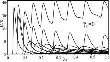
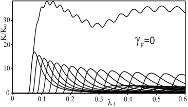
Figure 6: Absorption coefficient $K/K_{0}$, Eq. (60), consisting of a sum of the first partial contributions vs the energy $\lambda=\lambda_{1}$ of the optical interband transitions for the Lifshits-Slezov distribution, using the functions $f_{\nu,\nu^{\prime}}^{h\to e}(u)$ for GaAs $(h\to e)$ without electric field: for ensemble of OSQDs $\bar{c}=0.5$, $a=2.5$ (left panel) and for ensemble of PSQDs $\bar{a}=0.5$, $c=2.5$ (right panel).

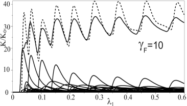
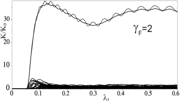
Figure 7: The same as in Fig. 6, but in the presence of electric field $2\gamma_{F}\!=\!F/F_{0}^{*}$. For comparison, the corresponding absorption coefficient without electric field is given by dashed line.

For the Lifshits-Slezov distribution Figs. 6 and 7 display the total absorption coefficients ${\tilde{K}(\tilde{\omega}^{ph})}/{\tilde{K}_{0}}$ and the partial absorption coefficients ${\tilde{K}_{\nu,\nu}(\tilde{\omega}^{ph})}/{\tilde{K}_{0}}$, that form the corresponding partial sum (60) over a fixed set of quantum numbers $\nu,\nu^{\prime}$ at $m=-m^{\prime}=0$. As a result of averaging (59) a series of curves with finite with and height are observed instead of a series of $\delta$-functions. One can see that the summation over the quantum numbers $n_{o}=n_{zo}+1=1,2,3,4,5$ (or $n_{p}=n_{\rho p}+1=1,2,3$) enumerating the nodes of the wave function with respect to the fast variable gives the corresponding principal maxima of the total AC for the ensemble of QDs with distributed dimensions of minor semiaxis, while the summation over the quantum number $n_{\rho o}=0,1,2,3,...,8$ (or $n_{zp}=0,1,2,...,15$) that labels the nodes of the wave function with respect to the slow variable leads to the increase of amplitudes of these maxima and to secondary maxima arising in the case of sparer energy levels of IPBM of OSQDs (or PSQDs).

In the regime of strong dimensional quantization the frequencies of the interband transitions ($h\to e$) in GaAS between the levels $n_{o}=1,n_{\rho o}=0,m=0$ for OSQD or $n_{p}=1,n_{zp}=0,m=0$ for PSQD at the fixed values $\tilde{a}=2.5a_{e}$ and $\tilde{c}=0.5a_{e}$ for OSQD or $\tilde{a}=0.5a_{e}$ and $\tilde{c}=2.5a_{e}$ for PSQD, are equal to $\Delta\tilde{\omega}^{ph}_{100}/(2\pi)=16.9$THz at $\gamma_{F}=0$ and $\Delta\tilde{\omega}^{ph}_{100}/(2\pi)=15.9$THz at $\gamma_{F}=10$, or $\Delta\tilde{\omega}^{ph}_{100}/(2\pi)=33.3$THz at $\gamma_{F}=0$ and $\Delta\tilde{\omega}^{ph}_{100}/(2\pi)=31.5$THz at $\gamma_{F}=2$, where $\Delta\tilde{\omega}^{ph}_{100}/(2\pi)=(2\pi\hbar)^{-1}(\tilde{W}_{100,100}-\tilde{E}_{g})$ corresponds to the IR spectral region 79 ; 79a , taking the band gap value $(2\pi\hbar)^{-1}\tilde{E}_{g}=346$ THz into account. In Fig. 7 one can see the quantum-confined Stark effect that consist in the reduction of the absorption energy (light frequency) at the expense of lowering the energy of both (e) and (h) bound states due to the electric field effect. The total ACs at $F\neq 0$, shown by solid lines, qualitatively correspond to the total AC at $F=0$, shown by dashed lines, but have lower magnitudes and smooth behavior, in spite of the additional contribution to the partial ACs of the overlap integral (58) from the interband transition $n_{zo}\neq n_{zo}^{\prime}$ or $n_{zp}\neq n_{zp}^{\prime}$ in OSQD or PSQD, also shown in Fig. 7.

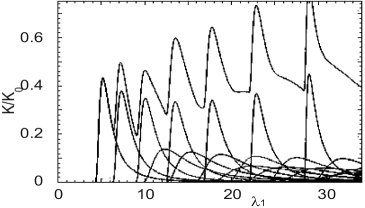
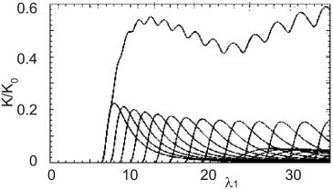
Figure 8: The same as in Fig. 6, but for InSb $(hh\to e)$ interband transition.

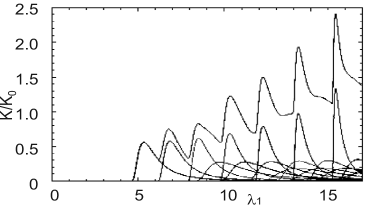
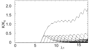
Figure 9: The same as in Fig. 6, but for InSb $(lh\to e)$ interband transition.

At the same parameters of the QDs the frequencies of the interband transitions ($lh\to e$) in InSb are equal to $\Delta\tilde{\omega}^{ph}_{100}/(2\pi)=68.5$THz for OSQD or $\Delta\tilde{\omega}^{ph}_{100}/(2\pi)=87.2$THz for PSQD, while the frequencies of the interband transitions ($hh\to e$) in InSb are equal to $\Delta\tilde{\omega}^{ph}_{100}/(2\pi)=78.6$THz for OSQD or $\Delta\tilde{\omega}^{ph}_{100}/(2\pi)=102$THz for PSQD. These values correspond to the infrared spectral region with longer wavelength, similar to  Hayk11 , with the band gap value $(2\pi\hbar)^{-1}\tilde{E}_{g}=44$THz taken into account. One can see that the behavior of total ACs for parabolic dispersion law for IPBM of InSb, shown in Fig. 8, is similar to that for GaAs (Fig. 6), while the behavior of AC for nonparabolic dispersion law, shown in Fig. 9, is essentially different. In particular, for OSQDs it grows faster with increasing $\lambda_{1}$, while for PSQDs it goes to a plateau before starting to grow. Indeed, with increasing quantum numbers $n_{\rho o}$ or $n_{zp}$ that characterize the excitation of slow motion, the maxima of partial ACs decrease for parabolic dispersion law, while for the nonparabolic one the maxima of partial ACs increase.

With decreasing semiaxis the threshold energy increases, because the “effective” band gap width increases, which is a consequence of the dimensional quantization enhancement. Therefore, the above frequency is greater for PSQD than for OSQD, because the SQ implemented in two direction of the plane (x,y) is effectively larger than that in the direction of the $z$ axis solely at similar values of semiaxes. Higher-accuracy calculations reveal an essential difference in the frequency behavior of the AC for interband transitions in systems of semiconductor OSQDs or PSQDs having a distribution of minor semiaxes, which can be used to verify the above models.

VII Conclusion

The 3-D BVP for spheroidal quantum dots with respect to fast and slow variables of cylindrical coordinates was reduced by Kantorovich or adiabatic method to BVP for set of second-order differential equations (ODE) with effective potentials given in the analytic form with respect to the slow variable, using the basis function of fast variables, that depended on the slow variable as a parameter. Separation of variables of 3D BVP in spheroidal coordinates provides exact classification of energy eigenvalues by means of nodes of eigenfunctions which transforms exactly to an adiabatic classification of eigensolutions of a diagonal approximation of ODE at small parameter, i.e. ratio of minor and major semiaxes of oblate or prolate spheroid. The effective potential of a crude diagonal adiabatic approximation (CDAA) of the ODE has been approximated by power expansions by slow variable. Energy eigenvalues and eigenfunctions of the BVP for CDAA were sought in expansions over eigenfunctions of 2D or 1D oscillator with adiabatic frequencies and power of small parameter by the PT. Required coefficients of these expansion were calculated in analytical form as polynomials of the sets of adiabatic quantum numbers.

To specify the region of the model parameters, in which the PT asymptotic series are valid, we we compared the PT results with those of numerical calculations carried out with required accuracy. The PT eigensolutions were used in analytic evaluation of the photoabsorption coefficient for ensembles of oblate and prolate spheroidal QDs with given random distribution of small semiaxes without and with small values of external electric fields. In general case for calculation $f_{\nu,\nu^{\prime}}(u)$ by formula (53), (56), or (57) we used eigenvalues calculated numerically with given accuracy and we evaluated the coefficients of expansion like (61) by the method of least squares and by the polynomial interpolation in the case of parabolic and nonparabolic dispersion laws, respectively. Note, in the case of numerical calculations of the photoabsorption coefficient the required derivatives of eigenenergies and eigenfunctions with respect to a parameter, e.g., the small semiaxis, can be calculated also with the help of the numerical algorithms ODPEVP ; progr07 .

The elaborated methods, symbolic-numerical algorithms (SNAs) and programs  Yu2 ; CASC10 ; JPCONF ; Yaf10 ; Yaf12 ; kantbp ; ODPEVP ; Yu3 ; Yu4 ; Yu5 ; progr07 ; Yu8 ; Yu9 can be applied for solving the BVPs of discrete and continuous spectra of the Schrödinger-type equations and the analysis of spectral and optical characteristics of QWs, QWr’s and QD’s in external fields, as well as the spectra of models of deformed nuclei DGZ2011 .

This work was partially supported by the RFBR Grants No 10-02-00200 and 11-01-00523.

References

- (1) D. Bimberg, M. Grundman, and N. Ledentsov, Quantum Dot Heterostructures (Wiley, New-York, 1999).
- (2) P. Harrison, Quantum Well, Wires and Dots. Theoretical and Computational Physics of Semiconductor Nanostructures (Wiley, New York, 2005).
- (3) Zh. Alferov, Semiconductors 32, 1 (1998).
- (4) Li Bin et al, Phys. Lett. A 367, 493 (2007).
- (5) G. Lamouche and Y Lépine, Phys. Rev. B 49, 13452 (1994).
- (6) H.A. Sarkisyan, Mod. Phys. Lett. B 16, 835 (2002).
- (7) K.G. Dvoyan et al, Nanoscale Res. Lett. 4, 106 (2009); Proc. SPIE 7998, 79981F (2010).
- (8) K.G. Dvoyan et al, Nanoscale Res. Lett. 2, 601 (2007).
- (9) S. López et al, Physica E 40 , 1383 (2008).
- (10) M. Barseghyan, A. Kirakosyan, and C. Duque Eur. Phys. J. B 72, 521 (2009).
- (11) A. Gharaati and R. Khordad, Superlattices Microstruct 48, 276 (2010).
- (12) I. Filikhin, V. M. Suslov, and B. Vlahovic Phys. Rev. B 73, 205332 (2006).
- (13) I. Filikhin el al, Physica E 41, 1358 (2009).
- (14) Al.L. Efros, A.L. Efros, Sov. Phys. Semicond. 16, 772 (1982).
- (15) I.M. Lifshits and V.V. Slezov, Sov. Phys. JETF. 35, 479 (1958).
- (16) K. Moiseev et al, Tech. Phys. Lett. 33, 295 (2007).
- (17) K. Moiseev et al, Semiconductors 43, 1102 (2009).
- (18) E.O. Kane, J. Phys. Chem. Sol. 1, 249 (1957).
- (19) B. Askerov, Electronic Transport Phenomena in Semiconductors (Nauka, Moscow ,1985).
- (20) E. Kazaryan, A. Meliksetyan, and H. Sarkisyan, Tech.Phys.Lett. 33, 964 (2007).
- (21) E. Kazaryan, A. Meliksetyan, and H. Sarkisyan, J. Comput. Theor. Nanosci. 7, 486 (2010).
- (22) M.S. Atonyan et al, Physica E 43, 1592 (2011).
- (23) V.L. Derbov et al Izvestia Saratov University, Serie Fizika 10, 4 (2010)(in Russian)
- (24) A.A. Gusev et al, Lect. Notes Comp. Sci. 6244, 106 (2010).
- (25) A.A. Gusev et al, J. Phys. Conf. Ser. 248, 012047–1–8 (2010).
- (26) A.A. Gusev et al, Phys. Atom. Nucl. 73, 352 (2010).
- (27) A.A. Gusev et al, Phys. Atom. Nucl. 75, (2012) accepted.
- (28) O. Chuluunbaatar et al, Comput. Phys. Commun. 177, 649 (2007).
- (29) O. Chuluunbaatar et al, Comput. Phys. Commun. 180, 1358 (2009).
- (30) O. Chuluunbaatar et al, Comput. Phys. Commun. 179, 685 (2008).
- (31) V. Gerdt et al, Lect. Notes Comp. Sci. 4194, 194 (2006).
- (32) O. Chuluunbaatar et al, Comput. Phys. Commun. 178, 301 (2008).
- (33) O. Chuluunbaatar et al, Lect. Notes Comp. Sci. 4770, 118 (2007).
- (34) A.A. Gusev et al, Lect. Notes Comp. Sci. 6885, 175 (2011).
- (35) S. Vinitsky et al, Progr. Comp. Software 33, 105 (2007).
- (36) J.E. Lennard-Jones, Proc. Roy. Soc. A 129, 598 (1930); J. Lond. Math. Soc. 6, 290 (1931); N. Mott and I. Sneddon, Wave Mechanics and its Applications (Clarendon, Oxford, 1948).
- (37) M. Abramowitz and I.A. Stegun, Handbook of Mathematical Functions (Dover, New York, 1965); http://dlmf.nist.gov/ NIST Digital Library of Mathematical Functions.
- (38) K. Helfrich, Theoret. chim. Acta (Berl.) 24,271 (1972).
- (39) E. M. Kazaryan, L. S. Petrosyan, and H. A. Sarkisyan, Physica E 16, 174 (2003).
- (40) M. Zoheir, A. Kh. Manaselyan, and H. A. Sarkisyan, Physica E 40, 2945 (2008).
- (41) M. Dobrowolski et al, Int. J. Mod. Phys. E. 20, 500 (2011).