Abstract

A model of a cloud formed by massive strings is used as a source of Bianchi type II. We assumed that the expansion $(\theta)$ in the model is proportional to the shear $(\sigma)$. To get exact solution, we have considered the equation of state of the fluid to be in the stiff form. It is found that the bulk viscosity plays a very important rule in the history of the universe. In presence of bulk viscosity the particles dominate over strings whereas in absence of it, strings dominate over the particles which is not in consistence with the recent observations. Also we observe that the viscosity caused the expansion of the universe to be accelerating. Our models are evolving from an early decelerating phase to a late time accelerating phase. The physical and geometrical behavior of these models are discussed.

keywords: LRS Bianchi type II models, Stiff Fluid, Massive String
PACS: 98.80.-k, 98.80.Cq, 04.20.-q, 04.20.Jb

1 Introduction

In recent years, there has been considerable interest in the study of the role of cosmic strings in the evolution of the universe, specially at it’s early epoches. One of the predictions of Grand Unified Theories (GUT) is that the universe underwent a phase transition as the temperature falls down below the $T_{GUT}\backsim 10^{28}K$ when the age of universe was $t_{GUT}\backsim 10^{-36}s$ (Zel’dovich et al. 1975; Kibble. 1980; Everett. 1981; Vilenkin. 1981). There is a loss of symmetry when the universe undergoes the GUT phase transition at $t_{GUT}$. At $T<T_{GUT}$, the symmetry between the strong and electro-weak forces spontaneously broken. The phase transitions associated with loss of symmetry leads to the formation of topological defects such as domain walls, cosmic strings, monopoles, etc. As mentioned by Kibble (1976), cosmic strings which are important topologically stable defects, might be created during a phase transition in the early universe. Although at the present time the existence of the cosmic strings can not be detected through our observations, their existence in the early epoches of cosmic evolutions is a well established fact. Zel’dovich (1980) was believed that the vacuum strings may generate density fluctuations sufficient to explain the galaxy formation. Since the cosmic strings have coupled stress-energy to the gravitational field, the study of gravitational effects of such strings seems to be interesting. The general relativistic treatment of strings was initiated by Letelier (1979, 1983). Here we have considered gravitational effects, arisen from strings by coupling of stress energy of strings to the gravitational field. Letelier (1979) defined the massive strings as the geometric strings (massless) with particles attached along its expansions.
As noted by Belinchon (2009), the string that form the cloud are the generalization of Takabayasi s relativistic model of strings (called $p$-strings). Therefore, a cloud model of strings is a model in which we have particles and strings together. However, since there is not any observational evidence for the exitance of the cosmic strings at the present time, one can eliminate the strings and end up with a cloud of particles at the present time of evolution of the universe (Banerjee et al. 1990; Yadav et al. 2007; Saha and Visinescu. 2008, 2010).

Most cosmological models assume that the matter in the universe can be describe by ’dust’ (a pressure-less distribution) or at best a perfect fluid. To have realistic cosmological models we should consider the presence of a material distribution other than a perfect fluid. Cosmological models of a fluid with viscosity play a significant role in the study of evolution of universe. The viscosity mechanism in cosmology can account for high entropy per baryon of the present universe (Weinberg. 1972). It is well known that at an early stage of the universe when neutrino decoupling occurs, the matter behaves like a viscous fluid (Kolb and Turner. 1990). Weinberg (1971, 1972) derived general formulae for bulk and shear viscosity and used these to evaluate the rate of cosmological entropy production. He deduced that the most general form of the energy-momentum tensor allowed by rotational and space-inversion invariance, contains a bulk viscosity term proportional to the volume expansion of the model. Padmanbhan and Chitre (1987) have also noted that viscosity may be of relevance for the future evolution of the Universe. If the coefficient of bulk viscosity decays sufficiently slowly, i.e., $\xi\sim\rho^{n},~{}n<\frac{1}{2}$, then the late epochs of the Universe will be viscosity dominated, and the Universe will enter a final inflationary era with steady-state character. Cosmological models with viscous fluid in early universe have been widely discussed in the literatures (for example see Pradhan et al. 2012; Pradhan and Lata. 2011; Pradhan. 2009; Pradhan and Shyam. 2009; Pradhan et al. 2008; Pradhan et al 2007; Pradhan et al. 2005 Yadav. 2011 a, b; Yadav et al. 2012 ).

The equation of state of a cosmic fluid is defined as the ratio of it’s pressure and energy density i.e $\omega=\frac{p}{\rho}$. A fluid in which $p=\rho$, is called “stiff fluid”. In this case, the speed of light is equal to speed of sound and its governing equations have the same characteristics as those of gravitational field (Zel’dovich. 1970). The relevance of stiff equation of state $\rho=p$ to the matter content of the universe in the early state of evolution of universe has first discussed by Barrow (1986). An exact solution of Einstein s field equation with stiff equation of state has investigated by Wesson (1978). Mohanty et al. (1982) have investigated cylindrically symmetric Zel dovich fluid distribution in General Relativity. Götz (1988) obtained a plane symmetric solution of Einstein s field equation for stiff perfect fluid distribution. Pradhan and Kumhar (2009) have investigated LRS Bianchi type II bulk viscous universe with decaying vacuum energy density in General Relativity. Recently A. K. Yadav et al. (2011) have investigated string L.R.S Bianchi type II universe in general relativity.

Bianchi type II space-time has a fundamental role in constructing cosmological models suitable for describing the early stages of evolution of universe. Asseo and Sol (1987) emphasized the importance of Bianchi type II universe. In the present paper we have considered a locally rotationally symmetric (LRS) model of spatially homogeneous Bianchi type-II cosmology. To obtain exact solutions, the field equations have been solved for the case when the equation of state of the fluid is in the stiff form. The paper is organized as follows. The metric and the field equations are presented in Section 2. In Section 3, we deal with solution of the field equations with cloud of strings. In Subsect. 3.1, we describe some physical and geometric properties of the model . In Subsect. 3.2, we give the solution in absence of bulk viscosity. A dark energy interpretation of the derived models is given in Section 4. Finally, in Section 5, concluding remarks are given.

2 The Metric and Field Equations

We consider the Bianchi type II metric in the form

$$ds^{2}=-dt^{2}+B^{2}(dy+xdz)^{2}+A^{2}(dx^{2}+dz^{2})$$ (1)

where $A$ , $B$ are functions of $t$ only. The energy-momentum tensor for a cloud of strings in presence of bulk viscosity is taken as

$$T_{ij}=(p+\rho)u_{i}u_{j}+pg_{ij}-\lambda x_{i}x_{j}+\xi\theta(g_{ij}+u_{i}u_{j}),$$ (2)

where $u_{i}$ and $x_{i}$ satisfy condition

$$u_{i}u^{i}=-x^{i}x_{i}=-1,\quad u^{i}x_{i}=0,$$ (3)

$p$ is the isotropic pressure, $\rho$ is the proper energy density for a cloud string with particles attached to them, $\lambda$ is the string tension density, $u^{i}$ the four-velocity of the particles, and $x^{i}$ is a unit space-like vector representing the direction of string. In a co-moving coordinate system, we have

$$u^{i}=(0,0,0,1),\quad x^{i}=(\frac{1}{B},0,0,0).$$ (4)

The particle density of the configuration is given by

$$\rho_{p}=R_{ij}u^{i}u^{j},$$ (5)

where $\rho_{p}$ is the rest energy density of the particles attached to the strings. The string tension density,$\lambda$, can take positive or negative values. Negative value of $\lambda$ represents a universe filled with no strings but only an anisotropic fluid whereas its positive value represents strings loaded with particles forming the surface of world sheet [8].

The Einstein’s field equations (with $8\pi G=1$ and $c=1$)

$$R_{ij}-\frac{1}{2}Rg_{ij}=-T_{ij}$$ (6)

for the metric (1) leads to the following system of equations:

$$G_{22}=2\frac{\ddot{A}}{A}+\frac{\dot{A}^{2}}{A^{2}}-\frac{3}{4}\frac{B^{2}}{A^{4}}=-p+\xi\theta+\lambda$$ (7)

$$G_{11}=G_{33}=\frac{\ddot{A}}{A}+\frac{\ddot{B}}{B}+\frac{\dot{A}\dot{B}}{AB}+\frac{1}{4}\frac{B^{2}}{A^{4}}=-p+\xi\theta$$ (8)

$$G_{00}=2\frac{\dot{A}\dot{B}}{AB}+\frac{\dot{A}^{2}}{A^{2}}-\frac{1}{4}\frac{B^{2}}{A^{4}}=\rho$$ (9)

where an overdot stands for the first and double overdot for second derivative with respect to $t$.
The spatial volume for LRS B-II is given by

$$V=A^{2}B.$$ (10)

We define $S=(A^{2}B)^{\frac{1}{3}}$ as the average scale factor of LRS B-II model (1) so that the Hubble’s parameter is given by

$$H=\frac{\dot{S}}{S}=\frac{1}{3}\left(\frac{2\dot{A}}{A}+\frac{\dot{B}}{B}\right).$$ (11)

We define the generalized mean Hubble’s parameter H as

$$H=\frac{1}{3}(H_{x}+H_{y}+H_{z}),$$ (12)

where $H_{x}=\frac{\dot{A}}{A}$, $H_{y}=\frac{\dot{B}}{B}$ and $H_{z}=H_{x}$ are the directional Hubble’s parameters in the directions of $x$, $y$ and $z$ respectively.

The deceleration parameter $q$ is conventionally defined by

$$q=-\frac{S\ddot{S}}{\dot{S}^{2}}.$$ (13)

The scalar expansion $\theta$, shear scalar $\sigma^{2}$ and the average anisotropy parameter $Am$ are defined by

$$\theta=\frac{2\dot{A}}{A}+\frac{\dot{B}}{B},$$ (14)

$$\sigma^{2}=\frac{1}{2}\left(\sum_{i=1}^{3}H_{i}^{2}-\frac{1}{3}\theta^{2}\right),$$ (15)

$$A_{m}=\frac{1}{3}\sum_{i=1}^{3}{\left(\frac{\triangle H_{i}}{H}\right)^{2}},$$ (16)

where $\triangle H_{i}=H_{i}-H(i=1,2,3).$

The Raychaudhuri equation reads

$$3\frac{\ddot{S}}{S}=-2\sigma^{2}+\frac{3}{2}\xi\theta-\frac{1}{2}(\rho+3p).$$ (17)

3 Solution of the Field Equations

The field equations (11)-(13) are a system of three equations with five unknown parameters $A,B,p,\rho,\lambda$. two additional constraints relating these parameters are required to obtain explicit solutions of the system. Firstly, we assume that the expansion $\theta$ in the model is proportional to the shear $\sigma$. This condition leads to

$$\frac{1}{\sqrt{3}}\left(\frac{\dot{A}}{A}-\frac{\dot{B}}{B}\right)=b\left(\frac{\dot{A}}{A}+2\frac{\dot{B}}{B}\right)$$ (18)

which yields to

$$\frac{\dot{A}}{A}=m\frac{\dot{B}}{B}$$ (19)

where $m=\frac{2b\sqrt{3}+1}{1-b\sqrt{3}}$ and $b$ are constants. Eq. (19), after integration, reduces to

$$A=B^{m},$$ (20)

Secondly, we assume that the fluid obeys the stiff fluid equation of state i.e

$$p=\rho.$$ (21)

Using eqs. (8) and (9) in eq. (21) we get

$$\frac{\ddot{A}}{A}+\frac{\ddot{B}}{B}+3\frac{\dot{A}\dot{B}}{AB}+\frac{\dot{A}^{2}}{A^{2}}-\xi\theta=0.$$ (22)

In view of eq. (20), eq. (21) is taken as

$$2\ddot{B}+4m\frac{\dot{B}^{2}}{B}=\frac{\chi}{(m+1)}B.$$ (23)

where I have assumed that the coefficient of bulk viscosity is inversely proportional to expansion i.e $\xi\theta=\chi$ (say) = constant.
Let $\dot{B}=f(B)$ which implies that $\ddot{B}=ff^{\prime}$, where $f^{\prime}=\frac{df}{dB}$. Hence (23) can be written as

$$\frac{d}{dB}(f^{2})+4m\frac{f^{2}}{B}=\frac{\chi}{(m+1)}B,$$ (24)

which on integration gives

$$dt=\frac{dB}{\sqrt{aB^{2}+bB^{-4m}}}.$$ (25)

Here, $a=\frac{\chi}{(2m^{2}+3m+1)}$ and $b$ is a positive integrating constant. Hence the model (1) is reduced to

$$ds^{2}=-\frac{dB^{2}}{aB^{2}+bB^{-4m}}+B^{2}(dx+zdy)^{2}+B^{2m}(dy^{2}+dz^{2}).$$ (26)

After using a suitable transformation of coordinates the model (26) reduces to

$$ds^{2}=-\frac{dT^{2}}{aT^{2}+bT^{-4m}}+T^{2}(dx+zdy)^{2}+T^{2m}(dy^{2}+dz^{2}).$$ (27)

3.1 The Geometric and Physical Significance of Model

Here we discuss some physical and kinematic properties of string model (27).
The pressure $(p)$, the energy density $(\rho)$, the string tension $(\lambda)$, and the particle density $(\rho_{p})$ for the model (27) are given by

$$p=\rho=\frac{m(m+2)}{2}\left[\frac{\chi}{(2m^{2}+3m+1)}+2bT^{-2(1+2m)}\right]-\frac{1}{4}\frac{1}{T^{2(2m-1)}},$$ (28)

$$\lambda=\frac{1}{2}\left(\frac{2m^{2}-3m+1}{2m^{2}+3m+1}\right)\chi-\frac{1}{T^{2(2m-1)}},$$ (29)

$$\rho_{p}=-\frac{1}{2}\left(\frac{m^{2}-5m+1}{2m^{2}+3m+1}\right)\chi+m(m+2)bT^{-2(1+2m)}+\frac{3}{4}\frac{1}{T^{2(2m-1)}}.$$ (30)

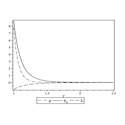
Figure 1: The plot of energy density $\rho$, particle density $\rho_{p}$ and tension density $\lambda$ Vs. $T$ for $m=2$, $\chi=0.1$ and $b=1$

From Eqs. (28) and (30), we observe that the energy density $\rho$ and the particle density $\rho_{p}$ are decreasing functions of time. This behavior of $\rho$ and $\rho_{p}$ is shown in figure 1. Also the energy conditions, $\rho\geq 0$ and $\rho_{p}\geq 0$ are satisfied under conditions

$$T^{-4}\left[4b+\frac{2\chi}{(2m^{2}+3m+1)}T^{2(2m+1)}\right]\geq\frac{1}{m(m+2)},$$ (31)

and

$$T^{-4}\left[-4m(m+2)b+\left(\frac{m^{2}-5m+1}{2m^{2}+3m+1}\right)\chi T^{2(2m+1)}\right]\geq\frac{3}{2},$$ (32)

respectively. Also $\lambda>0$ under

$$T>\left[2\left(\frac{2m^{2}+3m+1}{m^{2}-5m+1}\right)\frac{1}{\chi}\right]^{\frac{1}{2(2m-1)}}.$$ (33)

From Eq. (29), it is observed that $\lambda$ is an increasing function of time which is always negative and tends to zero at late time. It is pointed out by Letelier (1979) that $\lambda$ may be positive or negative. When $\lambda<0$, the string phase of the universe disappears i.e. we have an anisotropic fluid of particles. This behavior of tension density $\lambda$ is also depicted in figure 1.

To study the behavior of strings and particles in the universe here we define the following parameter

$$\frac{\rho_{p}}{|\lambda|}=\frac{-\frac{1}{2}\left(\frac{m^{2}-5m+1}{2m^{2}+3m+1}\right)\chi+m(m+2)bT^{-2(1+2m)}+\frac{3}{4}\frac{1}{T^{2(2m-1)}}}{|\frac{1}{2}\left(\frac{2m^{2}-3m+1}{2m^{2}+3m+1}\right)\chi-\frac{1}{T^{2(2m-1)}}|}.$$ (34)

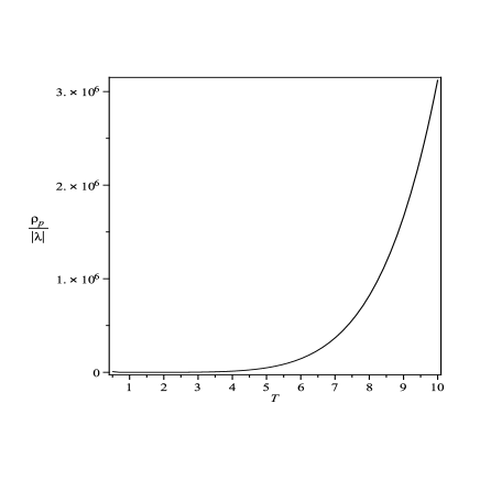
Figure 2: The plot of $\frac{\rho_{p}}{|\lambda|}$ Vs. $T$ for $m=2$, $\chi=0.1$ and $b=1$

As mentioned before, since strings are not observed at the present time of evolution of the universe, in principle we can eliminate the strings and end up with a cloud of particles. In other word, we can say the particles dominate over the strings at the present time of the evolution of the universe. Figure 2 is clearly shows that in the universe which is describe by the model (27) the strings dominate over the particle at initial time whereas the particles dominate over the strings at late time. Also it is worth to mention that from figures 2 and 3 we observe that at the initial time, when the universe is in the decelerating phase, the strings dominate over the particles ($\rho_{p}<\lambda$) whereas when the universe is in the accelerating phase particles dominate over the strings ($\rho_{p}>\lambda$). This is in agreement with the results obtained in Ref (Weinberg. 1976) and (Belinchon. 2009) and also with the astronomical observations which predict that there is no direct evidence of strings in the present-day universe.

The expressions for the scalar of expansion $\theta$, the average generalized Hubble’s parameter $H$, magnitude of shear $\sigma^{2}$, proper volume $V$, deceleration parameter $q$ and the average anisotropy parameter $A_{m}$ for the model (27) are given by

$$\theta=3H=(1+2m)\left[\frac{\chi}{2(2m^{2}+3m+1)}+bT^{-2(1+2m)}\right]^{\frac{1}{2}},$$ (35)

$$\sigma^{2}=\frac{(m-1)^{2}}{3}\left[\frac{\chi}{2(2m^{2}+3m+1)}+bT^{-2(1+2m)}\right],$$ (36)

$$V=T^{2m+1},$$ (37)

$$q=\frac{3}{2m+1}\left[\frac{2bT^{-2(1+2m)}-\frac{\chi}{2(2m^{2}+3m+1)}}{bT^{-2(1+2m)}+\frac{\chi}{2(2m^{2}+3m+1)}}\right],$$ (38)

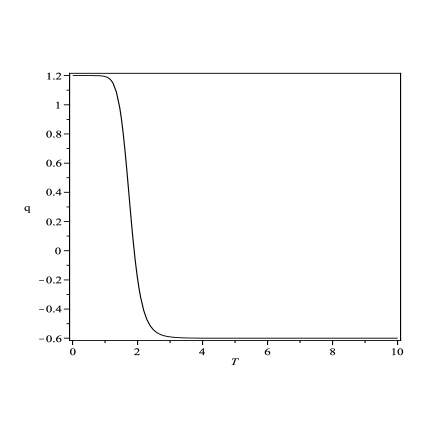
Figure 3: The plot of deceleration parameter $q$ Vs. $T$ for $m=2$, $\chi=0.1$ and $b=1$

$$A_{m}=2\left(\frac{1-m}{1+2m}\right)^{2}.$$ (39)

From (37) we observe that

$$q>0~{}~{}if~{}m>-\frac{1}{2}~{}\&~{}T<\left(\frac{2b}{a}\right)^{\frac{1}{2(1+2m)}}~{}~{}or~{}~{}m<-\frac{1}{2}~{}\&~{}T>\left(\frac{2b}{a}\right)^{\frac{1}{2(1+2m)}},$$ (40)

and

$$q<0~{}~{}if~{}m>-\frac{1}{2}~{}\&~{}T>\left(\frac{2b}{a}\right)^{\frac{1}{2(1+2m)}}~{}~{}or~{}~{}m<-\frac{1}{2}~{}\&~{}T<\left(\frac{2b}{a}\right)^{\frac{1}{2(1+2m)}}.$$ (41)

A positive sign of $q$ corresponds to the standard decelerating model whereas the negative sign $-1\leq q<0$ indicates the inflation. Recent observations show that the deceleration parameter of the universe is in the range $-1\leq q<0$ and the present day universe is undergoing an accelerated expansion. From figure 3 we observe that the model (27) successfully describes the expansion of our universe from decelerating to accelerating phase.
Also we note that for

$$T=\left[\frac{(1-m)\chi}{b(2m+7)(2m^{2}+3m+1)}\right]^{-\frac{1}{2(1+2m)}},$$

$q=-1$ as in the case of de-Sitter universe.

In absence of any curvature, matter energy density ($\Omega_{m}$) and dark energy ($\Omega_{\Lambda}$) are related by the equation

$$\Omega_{m}+\Omega_{\Lambda}=1,$$ (42)

where $\Omega_{m}=\frac{\rho}{3H^{2}}$ and $\Omega_{\Lambda}=\frac{\Lambda}{3H^{2}}$. Thus equation (42), reduce to

$$\frac{\rho}{3H^{2}}+\frac{\Lambda}{3H^{2}}=1.$$ (43)

Using equations (28) and (35), in equation (43), the cosmological constant is obtained as

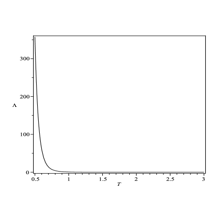
Figure 4: The plot of cosmological constant $\Lambda$ Vs. $T$ for $m=2$, $\chi=0.1$ and $b=1$

$$\Lambda=\left[\frac{(m-1)^{2}}{2(2m^{2}+3m+1)}\chi\right]+\frac{(m-1)^{2}}{3}bT^{-2(1+2m)}+\frac{1}{4}\frac{1}{T^{2(2m-1)}}.$$ (44)

From (44) we observe that $\Lambda$ is a decreasing function of time and is always positive for $m>-0.5$ and $m<-1$. This behavior of cosmological constant $\Lambda$ is clearly depicted in figure 4. Recent cosmological observations suggest the existence of a positive cosmological constant $\Lambda$ with the magnitude $\Lambda(G\hbar/c^{3})\approx 10^{-123}$. These observations on magnitude and red-shift of type Ia supernova suggest that our universe may be an accelerating one with induced cosmological density through the cosmological $\Lambda$-term. Thus, our model is consistent with the results of recent observations.
It is worth to mention that for $m=1$ from (44) we find

$$\Lambda=\frac{1}{4}\frac{1}{T^{2}}.$$ (45)

This supports the views in favor of the dependence $\Lambda\varpropto T^{-2}$ first expressed by Bertolami (1986 a, b) and later on observed by several authors (Rahman. 1990; Chen and Wu. 1990; Berman. 1990 a, b; Berman and Som. 1990; Pradhan and Kumar 2001). A relation like equation (45) also can be found in Brans-Dicke theories when one supposes variable gravitational and cosmological “constant” (Peebles and Ratra. 2003; Carmeli and Kuzmenko. 2002; Gasperini. 1987). We have derived the same variation of $\Lambda$ with time in string viscous cosmology in this article.

From the above results, it can be seen that the spatial volume is zero at $T=0$ and it increases with the increase of $T$ . This shows that the universe starts evolving with zero volume at $T=0$ and expands with cosmic time $T$ . In derived model, The energy density $\rho$, particle density $\rho_{p}$, tension density $\lambda$ and the cosmological constant $\Lambda$ become zero at $T\to\infty$ and tend to infinity at $T=0$. The model has the point-type singularity at $T=0$ (MacCallum. 1971). The expansion scalar and shear scalar all tend to zero as $T\to\infty$. The mean anisotropy parameter is uniform throughout whole expansion of the universe when $m\neq-\frac{1}{2}$ but for $m=-\frac{1}{2}$ it tends to infinity. This shows that the universe is expanding with the increase of cosmic time but the rate of expansion and shear scalar decrease to zero and tend to isotropic. Since $\frac{\sigma}{\theta}=$constant provided $m\neq-\frac{1}{2}$, the model does not approach isotropy at any time. But for $m=1$ our solution provide a totally isotropic universe.

3.2 Solutions in Absence of Bulk Viscous

In absence of bulk viscosity, i.e. $\chi\to 0$ or $a\to 0$, the metric (26) reduces to

$$ds^{2}=-\frac{dT^{2}}{bT^{-4m}}+T^{2}(dx+zdy)^{2}+T^{2m}(dy^{2}+dz^{2}).$$ (46)

The pressure $(p)$, the energy density $(\rho)$, the string tension $(\lambda)$, and the particle density $(\rho_{p})$ for the model (46) are given by

$$p=\rho=m(m+2)bT^{-2(1+2m)}-\frac{1}{4}\frac{1}{T^{2(2m-1)}},$$ (47)

$$\lambda=-\frac{1}{T^{2(2m-1)}},$$ (48)

$$\rho_{p}=m(m+2)bT^{-2(1+2m)}+\frac{3}{4}\frac{1}{T^{2(2m-1)}}.$$ (49)

Figure 5: The plot of energy density $\rho$, particle density $\rho_{p}$ and tension density $\lambda$ Vs. $T$ for $m=2$ and $b=1$

From eqs. (47) - (49) we observe that $\rho$, $\lambda$ and $\rho_{p}$ are decreasing functions of time and $\lambda$ is always negative. The energy conditions, $\rho\geq 0$ and $\rho_{p}\geq 0$ are satisfied under

$$T\geq\left(4bm(m+2)\right)^{\frac{1}{4}},$$ (50)

and

$$m>0~{}\&m>-2~{}~{}or~{}m<0~{}\&m<-2.$$ (51)

respectively. The behavior of $\rho$, $\lambda$ and $\rho_{p}$ are clearly depicted in Figures 5 as a representative case with appropriate choice of constants of integration and other physical parameters using reasonably well known situations.

From eqs. (48) and (49) we obtain

$$\frac{\rho_{p}}{|\lambda|}=bm(m+2)T^{-4}+3/4.$$ (52)

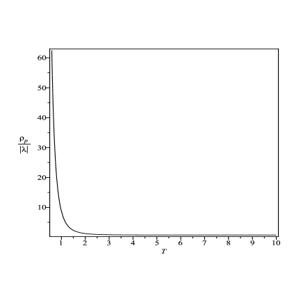
Figure 6: The plot of $\frac{\rho_{p}}{|\lambda|}$ Vs. $T$ for $m=2$ and $b=1$

Equation (52) obviously shows that $\frac{\rho_{p}}{|\lambda|}$ is a decreasing function of time i.e as time goes on, the strings dominate over the particles which in contradict with the result obtained in the first case in presence of bulk viscosity. This result is of course is not consistent with the astronomical observations, which predict that there is no direct evidence of strings in the present-day universe. Therefore, we conclude that the bulk viscosity may plays an important rule in creation of the particles from strings.

The expressions for the scalar of expansion $\theta$, the average generalized Hubble’s parameter $H$, magnitude of shear $\sigma^{2}$, proper volume $V$, deceleration parameter $q$ and the average anisotropy parameter $A_{m}$ for the model (46) are given by

$$\theta=3H=(1+2m)\sqrt{b}T^{-(1+2m)},$$ (53)

$$\sigma^{2}=\frac{(m-1)^{2}}{3}bT^{-2(1+2m)},$$ (54)

$$V=T^{2m+1},$$ (55)

$$q=\frac{6}{2m+1},$$ (56)

$$A_{m}=2\left(\frac{1-m}{1+2m}\right)^{2}.$$ (57)

From (56) we observe that $q>0$ if $m>-\frac{1}{2}$ and $q<0$ if $m<-\frac{1}{2}$. But from eq. (55) we observe that, $m<-\frac{1}{2}$ represents an accelerating collapsing universe with high blue shift. Since the recent observations (Riess et al. 2001) indicate that we live in an accelerating expanding universe with red shift, we conclude that in absence of bulk viscosity a universe with decreasing rate of expansion is the only possible scenario.

4 Dark Energy Interpretation of The Models

Fig. $3$ clearly shows that the presence of bulk viscosity in the cosmic fluid causes a decelerating to accelerating expansion of the universe. Also from Raychaudhuri’s equation. (17), we observe that that bulk viscosity can play the role of an agent that derive the present acceleration of the Universe.
In Eckart’s theory (1940) a viscous pressure is specified by

$${p}^{eff}=p+\Pi.$$ (58)

Here $\Pi=-\xi\theta$ is the viscous pressure. Therefore in our models the effective pressure (stiff fluid plus viscous fluid) can be written as

$$p^{eff}=p-\chi=\frac{m(m+2)}{2}\left[\frac{\chi}{(2m^{2}+3m+1)}+2bT^{-2(1+2m)}\right]-\frac{1}{4}\frac{1}{T^{2(2m-1)}}-\chi.$$ (59)

Using eqs. (28) and (59) the effective equation of state of the net fluid is obtained as

$$\omega^{eff}=\frac{p^{eff}}{\rho}=1-\frac{\chi}{\frac{m(m+2)}{2}\left[\frac{\chi}{(2m^{2}+3m+1)}+2bT^{-2(1+2m)}\right]-\frac{1}{4}\frac{1}{T^{2(2m-1)}}}.$$ (60)

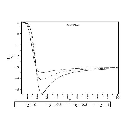
Figure 7: The plot of effective equation of state $\omega^{eff}$ Vs. $T$ for $m=1$ and $b=1$

The behavior of effective equation of state, $\omega^{eff}$, in terms of cosmic time $T$ is shown in Fig. $7$. It is observed that the $\omega^{eff}$ parameter is a decreasing function of $T$ and the rapidity of its decrease depends on the value of $\chi$. We see that in absence of bulk viscosity the models do not exhibit accelerating expansion (solid line) whereas in presence of viscosity our models exhibit a decelerating to an accelerating expansion. From both eq. (60) and Fig. 7 we observe that at the later stage of evolution, effective equation of state tends to the same constant value i.e $\omega^{eff}=1-\frac{2(2m^{2}+3m+1)}{m(m+2)}$ independent of the value of $\chi$.

5 Concluding Remarks

In this paper we have presented a new exact solution of Einstein s field equations for LRS Bianchi type II space-time with cloud of strings which is different from the other author s solution. In general the models are expanding, shearing and non-rotating. It is found that in present of bulk viscosity particles dominate over the strings at late time whereas in absence of viscosity strings dominate over the particles which is a contradictory result. In other hand, from Raychaudhuri’s equation (17) we observe that that bulk viscosity can play the role of an agent that derive the present acceleration of the Universe. Hence we conclude that the bulk viscosity plays an important role on the evolution of the universe. For a universe which was decelerating in past and accelerating at the present time, the deceleration parameter must show signature flipping (see the Refs. Padmanabhan and Roychowdhury. 2003; Amendola. 2003; Caldwell et al. 2006). Our models are evolving from an early decelerating phase to a late time accelerating phase (see, Figure 3) which is in good agreement with recent observations (Riess et al. 2001).

References

- [1] Abdel-Rahman, A.-M. M. 1990, Gen. Rel. Grav, 22, 655
- [2] Amendola, L. 2003, Mon. Not. R. Astron. Soc, 342, 221
- [3] Asseo, E., Sol, H. 1987, Phys. Rep, 148, 307
- [4] Banerjee, A., Sanyal, A. K., Chakraborty, S. 1990, Pramana. J. Phys, 34, 1
- [5] Barrow, J. D. 1986, Phys. Lett. B, 180, 335
- [6] Belinchon, J. A. 2009, Astrophys. Space Sci, 323, 307
- [7] Berman, M. S., Som, M. M. 1990, Int. J. Theor. Phys, 29, 1411
- [8] Berman, M. S, 1990, Int. J. Theor. Phys, 29, 567
- [9] Berman, M. S, 1990, Int. J. Theor. Phys, 29, 1419
- [10] Bertolomi, O. 1986, Nuovo Cimento, 93, 36
- [11] Bertolomi, O. 1986, Fortschr. Phys, 34, 829
- [12] Caldwell, R. R., Komp, W., Parker, L., Vanzella, D. A. T. 2006, Phys. Rev. D, 73, 023513
- [13] Carmeli, M., Kuzmenko, T. 2002, Int. J. Theor. Phys, 41, 131
- [14] Chen, W., Wu, Y. S. 1990, Phys. Rev. D, 41, 695
- [15] Eckart, C. 1940, Phys. Rev, 58, 919
- [16] Everett, A. E. 1981, Phys. Rev, 24, 858
- [17] Gasperini, M. 1987, Phys. Lett. B, 194, 347
- [18] Götz, G. 1988, Gen. Relativ. Gravit, 20, 23
- [19] Kibble, T. W. B. 1976, J. Phys. A: Math. Gen, 9, 1387
- [20] Kibble, T. W. B. 1980, Phys. Rep, 67, 183
- [21] Kolb, E. W., Turner, M. S. 1990, The Early Universe, Addison-Wesley
- [22] Letelier, P. S. 1979, Phys. Rev. D, 20, 1294
- [23] Letelier, P. S. 1983, Phys. Rev. D, 28, 2414
- [24] MacCallum, M. A. H. 1971, Commun. Math. Phys, 20, 57
- [25] Mohanty, G., Tiwari, R. N., Rao, J. R. 1982, Int. J. Theo. Phys, 21, 105
- [26] Padmanabhan, T., Roychowdhury. 2003, Mon. Not. R. Astron. Soc, 344, 823
- [27] Padmanabhan, T., Chitre, S. M. 1987, Phys. Letters A. 120, 433
- [28] Peebles, P. J. E., Ratra, B. 2003, Rev. Mod. Phys, 75, 559
- [29] Pradhan, A., Kumar, A. 2001, Int. J. Mod. Phys. D, 10, 291
- [30] Pradhan, A., Kumhar, S. S., Jotania, K. 2012, Polestin. J. Mathematics, 1 (2), 118
- [31] Pradhan, A., Lata, S. 2011, Elect. J. Theor. Phys, 8, 153
- [32] Pradhan, A. 2009, Comm. Theor. Phys, 51, 367
- [33] Pradhan, A., Shyam, S. S. 2009, Int. J. Theor. Phys, 48, 1466
- [34] Pradhan, A., Kumhar, S. S. 2009, Int. J. Theor. Phys, 48, 1466
- [35] Pradhan, A., Jotania, K., Singh, A. 2008, Braz. J. Phys, 38, 167
- [36] Pradhan, A., Rai, A., Singh, S. K. 2007, Astrophys. Space Sci, 312, 261
- [37] Pradhan, A., Yadav, A. K., Yadav, L. 2005, Czch, J. Phys, 55, 503
- [38] Riess, A. G., et al. 2001, Astrophys. J, 560, 49
- [39] Saha, B., Rikhvitsky, V., Visinescu, M. 2010, Cent. Eur. J. Phys, 8, 113
- [40] Saha, B., Visinescu, M. 2008, Astrophys. Space Sci, 315, 99
- [41] Vilenkin, A. 1981, Phys. Rev. D, 24, 2082
- [42] Weinberg, S. 1972, Gravitation and Cosmology, Wiley and Sons, New York
- [43] Weinberg, S. 1971, Astrophys. J, 168, 175
- [44] Wesson, P. S. 1978, J. Math. Phys, 19, 2283
- [45] Yadav, A. K. 2011, Rom. Rep. Phys, 63, 862
- [46] Yadave, A. K. 2011, arXiv: 1009.3867v2
- [47] Yadav, A. K., Pradhan, A., Singh, A. K. 2012, Astrophys. Space Sci, 337,379
- [48] Yadav, A. k., Pradhan, A., Singh, A. 2011, Roman. J. Phys, 56, 1019
- [49] Yadav, M. K., Rai, A., Pradhan, A. 2007, Int. J. Theor.Phys, 46, 2677
- [50] Zel’dovich, Ya. B. 1980, Mon. Not. R. Astron. Soc, 192, 663
- [51] Zel’dovich, Ya. B., Kobzarev, I. Yu., Okun, L.B. 1975, Eksp. Teor. Fiz, 67, 3
- [52] Zel’dovich, Ya. B. 1970, Mon. Not. R. Astron. Soc, 160