Pattern formation driven by cross–diffusion
in a 2D domain

Abstract

In this work we investigate the process of pattern formation in a two dimensional domain for a reaction-diffusion system with nonlinear diffusion terms and the competitive Lotka-Volterra kinetics. The linear stability analysis shows that cross-diffusion, through Turing bifurcation, is the key mechanism for the formation of spatial patterns . We show that the bifurcation can be regular, degenerate non-resonant and resonant. We use multiple scales expansions to derive the amplitude equations appropriate for each case and show that the system supports patterns like rolls, squares, mixed-mode patterns, supersquares, hexagonal patterns.

1 Introduction

The aim of this paper is to study the pattern formation for the reaction-diffusion system:

$$\begin{split}\frac{\partial u}{\partial t}=&\mathbf{\nabla}\cdot\mathbf{J}_{1}+\Gamma u(\mu_{1}-\gamma_{11}u-\gamma_{12}v),\\ \frac{\partial v}{\partial t}=&\mathbf{\nabla}\cdot\mathbf{J}_{2}+\Gamma v(\mu_{2}-\gamma_{21}u-\gamma_{22}v).\end{split}$$ (1.1a)

where the fluxes $\mathbf{J}_{i}$ have the following nonlinear expressions:

$$\begin{split}\mathbf{J}_{1}=&\mathbf{\nabla}(u(c_{1}+a_{1}u+bv)),\\ \mathbf{J}_{2}=&\mathbf{\nabla}(v(c_{2}+a_{2}v+b_{2}u)).\end{split}$$ (1.1b)

Here $u(\mathbf{x},t)$ and $v(\mathbf{x},t)$ are the population densities of two competing species, and $\mathbf{x}\in\Omega$ with $\Omega=[0,L_{x}]\times[0,L_{y}]$. The above system is supplemented with initial data and following Neumann boundary conditions:

$$\mathbf{n}\cdot\mathbf{J}_{1}=\mathbf{n}\cdot\mathbf{J}_{2}=0\qquad\mbox{when}\quad\mathbf{x}\in\partial\Omega\;.$$

The nonlinear diffusion terms describe the tendency of the species to diffuse, when densities are high, faster than predicted by the usual linear diffusion towards lower density areas. The parameters $a_{i}$ and $c_{i}$ are the self-diffusion and the linear diffusion coefficients respectively, while the parameters $b$ and $b_{2}$ are the cross-diffusion coefficients. For two competing species it is natural to suppose all these parameters to be non negative.

The constants $\gamma_{ij}\geq 0$ are the competitive interaction coefficients, the constants $\mu_{i}$ are the rates at which each species would grow in absence of competition, while the parameter $\Gamma$ regulates the size of the spatial domain (or the relative strength of reaction terms).

Since the seminal paper of Turing [45], reaction-diffusion equations are one of the best-known theoretical models explaining self-regulated pattern formation in many different areas of physics, chemistry, biology, geology, etc. Turing showed that the interplay of diffusion and kinetics can destabilize the uniform steady state and generate stable, stationary concentration patterns. However, if the model has a trivializing kinetics, as it is the case for competitive Lotka-Volterra kinetics, classical diffusion is not sufficient to destabilize the equilibria, no matter what the diffusion rates are, and no pattern formation can be observed. Thus, in order to model segregation keeping a simple form for the kinetic term, Shigesada, Kawasaki and Teramoto [43] proposed the nonlinear evolution system (1.1).

Strongly coupled parabolic systems with nonlinear diffusion terms of the form given in (1.1) have been used to model different physical phenomena and appeared in many context like chemotaxis [31, 2], ecology [27, 44, 30, 51, 24, 21, 40], social systems [35, 50, 19], turbulent transport in plasmas [17], drift-diffusion in semiconductors [11, 7, 16], granular materials [4, 23] and cell division in tumor growth [42].

The system (1.1) has been extensively investigated from the mathematical point of view. In [9, 10, 47] global existence and regularity results have been obtained, while in [32] the existence of non constant steady state solutions in the time independent case was investigated. The proof of existence and stability of traveling wave solutions has been obtained in [49]. The existence of positive steady-state solutions in relation to large cross-diffusion coefficients has been discussed in [39]. Some families of exact solutions have been constructed in [12] using the Lie symmetry approach while Lyapunov functionals have been used in [20, 36] to obtain stability and instability criteria of the zero solutions of cross-diffusion systems. From the numerical viewpoint different numerical schemes have been proposed to solve reaction-diffusion systems with nonlinear diffusion, see [3, 5, 22, 25, 8, 28].

The importance of the cross-diffusion, relatively to pattern formation, is extensively discussed in [1, 46] from both the experimental and the theoretical point of view. In these papers the authors report many experiments of interest to chemists where cross-diffusion effects can be significant: they obtain the minimal conditions for pattern formation in the presence of linear cross-diffusion terms, demonstrating that relatively small values of cross-diffusion parameters can lead to spatiotemporal pattern formation provided that the kinetics is sufficiently nonlinear.

The focus of this work is to describe the mechanisms of pattern formation for the system (1.1) with homogeneous Neumann boundary conditions in a 2D domain. The crucial difference with the 1D case analyzed in [26] consists in the possibility that bifurcation occurs via a simple or a multiple eigenvalue, see below and [33, 38, 15]. We shall perform a weakly nonlinear analysis close to the bifurcation state using the multiple scales analysis: this will give the equations which rule the evolution of the pattern amplitude near the threshold. A systematic approach to derive the normal forms and the correspondent amplitude equations for flows at local bifurcations can be found in [14, 34, 29, 13, 28]. A comparison between different methods of weakly nonlinear analysis for several prototype reaction-diffusion equations is given in [48].

The paper is organized as follows: in Section 2 a linear stability analysis of the system (1.1) is performed and the cross-diffusion is proved to be responsible for the initiation of spatial patterns. In Section 3 the amplitude and the form of the pattern close to the bifurcation threshold are investigated by using a weakly nonlinear multiple scales analysis. In particular, when the homogeneous steady state bifurcates to spatial pattern at a simple eigenvalue, we derive the cubic and the quintic Stuart-Landau equation which rules the evolution of the amplitude of the most unstable mode in the supercritical and subcritical case respectively. In these cases the system supports patterns such rolls and squares. On the other hand, when the bifurcation occurs via a double eigenvalue more complex patterns arise due to the interaction of different modes (for this reason they are called mixed mode patterns). The corresponding evolution systems for the amplitudes of the pattern are obtained and analyzed. A particular type of mixed mode patterns are the hexagonal patterns, which arise when a resonance condition holds. The evolution system for the amplitudes of the hexagonal patterns is proved to show bi-stability and the phenomenon of hysteresis can be observed.

In all the considered cases the solutions predicted by the weakly nonlinear analysis are compared with the numerical solutions of the original system. Close to the threshold they show a good agreement.

2 Cross-diffusion driven instability

In this section we shall investigate the possibility of pattern appearance for the system (1.1). In Subsection 2.1 we shall determine the critical value for the bifurcation parameter and the critical wavenumber via linear stability analysis. This will be done ignoring the geometry of the domain and the role played by the boundary conditions.

This role will be considered in Subsection 2.2 where we shall obtain the range of the unstable wavenumbers of allowable patterns strictly depending on the domain geometry. Since the degeneracy phenomenon can occur, the situation is much more involved than in the 1-D domain treated in [26] .

2.1 Main results on the destabilization mechanism

In order to stress the role played by the cross diffusion term in the pattern forming process, the kinetics is chosen of the simplest form, namely the competitive Lotka-Volterra, i.e. all $\gamma_{ij}>0$. We shall only analyze the coexistence equilibrium:

$$(u_{0},v_{0})\equiv\left(\displaystyle\frac{\mu_{1}\gamma_{22}-\mu_{2}\gamma_{12}}{\gamma_{11}\gamma_{22}-\gamma_{12}\gamma_{21}},\displaystyle\frac{\mu_{2}\gamma_{11}-\mu_{1}\gamma_{21}}{\gamma_{11}\gamma_{22}-\gamma_{12}\gamma_{21}}\right),$$ (2.1)

as this is the only steady state relevant for pattern formation. Therefore in this paper we shall assume the following conditions:

$$\mu_{1}\gamma_{22}-\mu_{2}\gamma_{12}>0,\qquad\mu_{2}\gamma_{11}-\mu_{1}\gamma_{21}>0,\qquad\gamma_{11}\gamma_{22}-\gamma_{12}\gamma_{21}>0\,.$$ (2.2)

The third condition (weak interspecific competition) is necessary for the stability of the equilibrium (2.1).

Upon linearization of the system (1.1) in a neighborhood of $(u_{0},v_{0})$, namely:

$$\dot{\textbf{w}}=\Gamma K\textbf{w}+D\nabla^{2}\textbf{w},\ \ \ \qquad\textrm{where}\qquad\textbf{w}=\left(\begin{array}[]{c}{u-u_{0}}\\ {v-v_{0}}\end{array}\right),$$ (2.3)

and where:

$$K = \left(\begin{array}[]{cc}-\gamma_{11}u_{0}&-\gamma_{12}u_{0}\\ -\gamma_{21}v_{0}&-\gamma_{22}v_{0}\end{array}\right),$$ (2.6)

$$D = \left(\begin{array}[]{cc}c_{1}+2a_{1}u_{0}+bv_{0}&bu_{0}\\ b_{2}v_{0}&c_{2}+2a_{2}v_{0}+b_{2}u_{0}\end{array}\right),$$ (2.9)

we look for solutions in the form $e^{i\mathbf{k}\cdot\mathbf{x}+\sigma t}$. Substitution in (2.3) leads to the following dispersion relation, which gives the eigenvalue $\sigma$ as a function of the wavenumber $k=|\mathbf{k}|$:

$$\sigma^{2}-g(k^{2})\sigma+h(k^{2})=0\;,$$ (2.10)

where

$$g(k^{2})=k^{2}\,{\rm tr}(D)-\Gamma\,{\rm tr}(K)\,,\qquad h(k^{2})={\rm det}(D)k^{4}+\Gamma qk^{2}+\Gamma^{2}{\rm det}(K)\;,$$ (2.11)

and

$$\begin{split}q=&\ \gamma_{11}u_{0}(2a_{2}v_{0}+c_{2})+\gamma_{22}v_{0}(2a_{1}u_{0}+c_{1})+bv_{0}(\gamma_{22}v_{0}-\gamma_{21}u_{0})\\ &+b_{2}u_{0}(\gamma_{11}u_{0}-\gamma_{12}v_{0})\;.\end{split}$$ (2.12)

For the Turing instability to be realized and spatial patterns to form, $Re(\sigma)$ must be greater than zero for some $k\neq 0$. Since the polynomial $g(k^{2})>0,\forall k\neq 0$ (in fact ${\rm tr}(K)<0$ being $(u_{0},v_{0})$ stable and ${\rm tr}(D)>0$), $Re(\sigma)$ will be positive for that $k\neq 0$ at which $h(k^{2})<0$. The steady state is marginally stable at some $k=k_{c}$ where:

$${\rm min}(h(k_{c}^{2}))=0.$$ (2.13)

As the minimum of $k$ is obtained when:

$$k_{c}^{2}=-\frac{\Gamma q}{2\,{\rm det}(D^{b^{c}})},$$ (2.14)

one has to require that $q$ can become negative. In the above formula the matrix $D^{b^{c}}$ is the matrix $D$ defined in (LABEL:2.3) evaluated at $b=b^{c}$.

From the expression (2.12) of $q$ where it is apparent that the first two terms are non negative, it follows that the only potential destabilizing mechanism is the presence of the cross-diffusion terms. Moreover only one of the last two terms in (2.12) can be negative, due to the conditions on positiveness and stability of $(u_{0},v_{0})$. Therefore when $\gamma_{22}v_{0}-\gamma_{21}u_{0}<0$ (verified in the hyperbolic sector $P_{1}$ on the left of Fig. 2.1), $b$ has a destabilizing effect and $b_{2}$ acts as a stabilizer. Alternatively, when $\gamma_{11}u_{0}-\gamma_{12}v_{0}<0$ (region $P_{2}$ on the left of Fig. 2.1), $b$ and $b_{2}$ exchange their role. In the remainder of this paper we shall choose the kinetic parameter set in the first case and the cross-diffusion coefficient $b$ as the bifurcation parameter.

Let us now write $q=-\alpha b+\beta$, where the positive quantities $\alpha$ and $\beta$ are defined as:

$$\begin{split}\alpha&=v_{0}(\gamma_{21}u_{0}-\gamma_{22}v_{0})\,,\\ \beta&=\gamma_{11}u_{0}(2a_{2}v_{0}+c_{2})+\gamma_{22}v_{0}(2a_{1}u_{0}+c_{1})+b_{2}u_{0}(\gamma_{11}u_{0}-\gamma_{12}u_{0})\,.\end{split}$$

Substituting $b=\beta/\alpha+\xi$ in the condition for the marginal stability (2.13) leads to the following equation for $\xi$:

$$\begin{split}\frac{\alpha^{2}}{4{\rm det}(K)}\,\xi^{2}-v_{0}(2a_{2}v_{0}+&c_{2})\xi-[v_{0}\beta/\alpha(2a_{2}v_{0}+c_{2})\\ +&(2a_{1}u_{0}+c_{1})(2a_{2}v_{0}+b_{2}u_{0}+c_{2})]=0.\end{split}$$ (2.15)

Then the critical bifurcation value is:

$$b^{c}=\beta/\alpha+\xi^{+},$$ (2.16)

where $\xi^{+}$ is the positive root of equation (2.15) in such a way that $q<0$.

The results of this section can be summarized in the following theorem.

Theorem 1

Suppose that $(u_{0},v_{0})$, as given in (2.1), is a stable equilibrium for the competitive kinetics of the system (1.1), i.e. assume conditions (2.2) to be valid.

Moreover assume that $\gamma_{11}u_{0}-\gamma_{12}v_{0}<0$. If:

$$b>b^{c},$$

where $b^{c}$ is defined in (2.16), then $(u_{0},v_{0})$ is an unstable equilibrium for the reaction-diffusion system (1.1).

An analogous statement would hold when $\gamma_{22}v_{0}-\gamma_{21}u_{0}<0$.

Proposition 2

Suppose that $(u_{0},v_{0})$ is a stable equilibrium for the competitive kinetics of the system (1.1).

If $\gamma_{22}v_{0}-\gamma_{21}u_{0}<0$, the Turing parameter space of instability is the bounded region $P_{1}$ on the left of Fig.2.1. Alternatively, if $\gamma_{22}v_{0}-\gamma_{21}u_{0}<0$, the Turing parameter space of instability is the bounded region $P_{2}$ .

2.2 Instability bands and degeneracy

When the domain is finite, the condition $b>b_{c}$ is not enough to see a pattern emerging. In this case, in fact, $k_{c}$ might not be a mode admissible for the domain and the boundary condition. However when $b>b^{c}$, there exists a range $(k_{1}^{2},k_{2}^{2})$ of unstable wavenumbers that make $h(k^{2})<0$ and, correspondingly, $Re(\sigma)>0$, see on the right of Fig.2.1. It is easy to see that the extremes of the interval of unstable wavenumbers, $k_{1}^{2}$ and $k_{2}^{2}$, where $h(k^{2})=0$, are proportional to $\Gamma$. It follows that $\Gamma$ must be big enough to find at least one of the modes allowed by the Neumann boundary conditions within the interval $[k_{1}^{2},k_{2}^{2}]$.

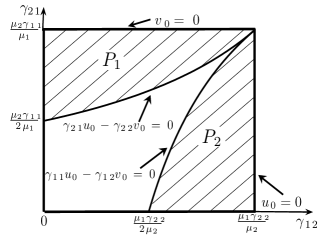
Figure 2.1: Left: Pattern forming regions in the plane $(\gamma_{12},\gamma_{21})$. Right: Growth rate of the $k$-th mode.

In a rectangular domain defined by $0<x<L_{x}$ and $0<y<L_{y}$, the solutions to the linear system (2.3) with Neumann boundary conditions are:

$${\bf w}=\sum_{m,n\in\mathbb{N}}\mathbf{f}_{mn}\,e^{\sigma({k}_{mn}^{2})\,t}\,\cos\left(\frac{m\pi}{L_{x}}\,x\right)\cos\left(\frac{m\pi}{L_{y}}\,y\right),$$ (2.17)

$$k_{mn}^{2}=\left(\frac{m\pi}{L_{x}}\right)^{2}+\left(\frac{n\pi}{L_{y}}\right)^{2},$$ (2.18)

where $\mathbf{f}_{m,n}$ are the Fourier coefficients of the initial conditions; the values $\sigma(k_{mn}^{2})$ are derived from the dispersion relation (2.10). The occurrence of a pattern emerging as $t$ increases, therefore depends on the existence of mode pairs $(m,n)$ such that:

$$k_{1}^{2}<k^{2}\equiv\phi^{2}+\psi^{2}<k_{2}^{2},\ {\rm where}\ \ \phi\equiv\frac{m\pi}{L_{x}},\ \ \psi\equiv\frac{n\pi}{L_{y}},$$ (2.19)

$$\sigma(k^{2})>0,$$ (2.20)

i.e. for $b>b^{c}$ and $\Gamma$ sufficiently large. In what follows we shall restrict ourselves to the case when there is only one unstable eigenvalue, admissible for the Neumann boundary conditions, that falls within the band $(k_{1},k_{2})$ in the sense of Eq.(2.19). We shall denote this admissible eigenvalue with $\bar{k}_{c}$ to distinguish from the critical value $k_{c}$.

In a two dimensional domain, given $\bar{k}_{c}\in[k_{1},k_{2}]$, one, two or more pairs $(m,n)$ may exist such that the condition

$$\bar{k}_{c}^{2}=\phi^{2}+\psi^{2}=\left(\frac{m\pi}{L_{x}}\right)^{2}+\left(\frac{n\pi}{L_{y}}\right)^{2}$$ (2.21)

is satisfied and in this case the eigenvalue $\sigma$ will have single, double or higher multiplicity respectively. The multiplicity of the eigenvalue, and therefore the type of linear patterns we could expect, strictly depends on the dimensions of the domain $L_{x}$ and $L_{y}$.

In Fig.2.2 we show the pattern which forms starting from an initial datum which is a random periodic perturbation about the steady state $(u_{0},v_{0})$. For the parameters we have picked for this simulation, one has $(u_{0},v_{0})\approx(1.67,0.92)$ while the critical value of the bifurcation parameter is $b^{c}=7.192$. In the rectangular domain with $L_{x}=\sqrt{2}\pi$ and $L_{y}=2\pi$ only the mode $\bar{k}_{c}^{2}=6$ is admitted by the boundary conditions. The eigenvalue predicted by the linear analysis is single: in fact there only exists the pair $(2,4)$ which satisfies the condition (2.18).

All the numerical simulations showed in this paper are performed by using spectral methods. Here we have employed $32$ modes both in the $x$ and in the $y$ axis. However the use of a higher number of modes in the scheme (we tested the method up to $128$ modes) does not appreciably affect the results. Notice that in all the figures representing the spectrum of the solutions, for a better presentation of the results, the amplitude of the zero mode, corresponding to the equilibrium solution, has been set equal to zero.

Figure 2.2: Left: The species $u$. Right: The species $v$. The parameters are $\mu_{1}=1.2$, $\mu_{2}=1$, $\gamma_{11}=0.5$, $\gamma_{12}=0.4$, $\gamma_{21}=0.38$, $\gamma_{22}=0.4$, $a_{1}=0.01$, $a_{2}=0.001$, $c_{1}=0.1$, $c_{2}=0.2$, $\Gamma=28.05$, $b_{2}=1.1$, $b=7.264>b^{c}=7.192$.

Figure 2.3: Spectrum of the numerical solutions in Fig. 2.2.

3 Weakly nonlinear analysis

In this section a weakly nonlinear analysis is carried out to obtain the amplitude equations describing the dynamics near the critical bifurcation state . The method of multiple scales (as introduced in [37]), together with an asymptotic analysis of the system close to its marginal stability are employed to determine the near-critical bifurcation structure of the patterns [14] .

Near the threshold the amplitude of the pattern evolves on a slow temporal scale, and therefore we shall introduce new scaled coordinates separating the fast time $t$ and slow time e.g. $T=\varepsilon t$; here the control parameter $\varepsilon$ will measure the distance of the system from bifurcation, see (3.11) below. The solution of the original system (1.1) is written as an expansion in $\varepsilon$ and the leading order term of this expansion is shown to be the product of the basic pattern (the critical solution of the linearized system (2.3)) and a slowly varying amplitude (see [28, 29]). We shall confine ourselves to patterns which are modulated in time but not in space, so that in our analysis we do not take into account the slow spatial scale.

If one defines the linear operator:

$$\mathcal{L}^{b}=\Gamma\,K+D^{b}\nabla^{2},$$ (3.1)

where $K$ and $D^{b}$ are given in (2.6) and (LABEL:2.3), and if one introduces the following bilinear operators acting on $(\mathbf{x},\mathbf{y})$ with $\textbf{x}\equiv(x^{u},x^{v})$ and $\textbf{y}\equiv(y^{u},y^{v})$:

$$\mathcal{Q}_{K}(\textbf{x},\textbf{y}) = \Gamma\left(\begin{array}[]{c}-2\gamma_{11}x^{u}y^{u}-\gamma_{12}(x^{u}y^{v}+x^{v}y^{u})\\ -2\gamma_{22}x^{v}y^{v}-\gamma_{21}(x^{u}y^{v}+x^{v}y^{u})\end{array}\right),$$ (3.4)

$$\mathcal{Q}_{D}^{b}(\textbf{x},\textbf{y}) = \left(\begin{array}[]{c}2a_{1}x^{u}y^{u}+b(x^{u}y^{v}+x^{v}y^{u})\\ 2a_{2}x^{v}y^{v}+b_{2}(x^{u}y^{v}+x^{v}y^{u})\end{array}\right),$$ (3.7)

the original system (1.1) can be rewritten separating the linear and the nonlinear part as follows:

$$\partial_{t}\textbf{w}=\mathcal{L}^{b}\textbf{w}+\frac{1}{2}\mathcal{Q}_{K}(\textbf{w},\textbf{w})+\frac{1}{2}\nabla^{2}\mathcal{Q}_{D}^{b}(\textbf{w},\textbf{w}),$$ (3.8)

with w defined as in (2.3).

Let us introduce the multiple time scales:

$$t=\frac{T_{1}}{\varepsilon}+\frac{T_{2}}{\varepsilon^{2}}+\frac{T_{3}}{\varepsilon^{3}}+\frac{T_{4}}{\varepsilon^{4}}+\dots$$ (3.9)

and expand accordingly both the solution ${\bf w}$ and the bifurcation parameter $b$:

$${\bf w} = \varepsilon{\bf w}_{1}+\varepsilon^{2}{\bf w}_{2}+\varepsilon^{3}{\bf w}_{3}+\varepsilon^{4}{\bf w}_{4}+O(\varepsilon^{5}),$$ (3.10)

$$b = b^{c}+\varepsilon b^{(1)}+\varepsilon^{2}b^{(2)}+\varepsilon^{3}b^{(3)}+\varepsilon^{4}b^{(4)}+O(\varepsilon^{5}).$$ (3.11)

Expansion (3.11) can be considered as the definition of the smallness parameter. In the rest of this paper, we shall always measure the distance from the threshold using, as unit, the critical value $b^{c}$. This means that, when different from zero, we shall set $b^{(i)}=b^{c}$. Substituting (3.9)-(3.11) into the full system (1.1), the following sequence of linear equations for $\mathbf{w}_{i}$ is obtained:

$$O(\varepsilon) :$$

$$\mathcal{L}^{b^{c}}{\bf w}_{1}=\mathbf{0},$$

$$O(\varepsilon^{2}) :$$ (3.16)

$$\mathcal{L}^{b^{c}}{\bf w}_{2}=\mathbf{F}=\frac{\partial{\bf w}_{1}}{\partial T_{1}}-\frac{1}{2}\left(\mathcal{Q}_{K}+\nabla^{2}\mathcal{Q}_{D}^{b^{c}}\right)(\mathbf{w}_{1},\mathbf{w}_{1})$$

$$\quad\quad\quad-b^{(1)}\left(\begin{array}[]{cc}v_{0}&u_{0}\\ 0&0\end{array}\right)\nabla^{2}{\bf w}_{1},$$

$$O(\varepsilon^{3}) :$$ (3.22)

$$\mathcal{L}^{b^{c}}{\bf w}_{3}=\mathbf{G}=\frac{\partial{\bf w}_{1}}{\partial T_{2}}+\frac{\partial{\bf w}_{2}}{\partial T_{1}}-\left(\mathcal{Q}_{K}+\nabla^{2}\mathcal{Q_{D}}^{b^{c}}\right)(\mathbf{w}_{1},\mathbf{w}_{2})$$

$$\quad\quad\quad-b^{(1)}\nabla^{2}\left(\begin{array}[]{c}u_{1}v_{1}\\ 0\end{array}\right)-\left(\begin{array}[]{cc}v_{0}&u_{0}\\ 0&0\end{array}\right)\left(b^{(1)}\nabla^{2}{\bf w}_{2}+b^{(2)}\nabla^{2}{\bf w}_{1}\right),$$

$$O(\varepsilon^{4}) :$$ (3.32)

$$\mathcal{L}^{b^{c}}{\bf w}_{4}=\mathbf{H}=\frac{\partial{\bf w}_{1}}{\partial T_{3}}+\frac{\partial{\bf w}_{2}}{\partial T_{2}}+\frac{\partial{\bf w}_{3}}{\partial T_{1}}-\left(\mathcal{Q}_{K}+\nabla^{2}\mathcal{Q_{D}}^{b^{c}}\right)(\mathbf{w}_{1},\mathbf{w}_{3})$$

$$\quad\quad\quad-\frac{1}{2}\left(\mathcal{Q}_{K}+\nabla^{2}\mathcal{Q_{D}}^{b^{c}}\right)(\mathbf{w}_{2},\mathbf{w}_{2})-b^{(1)}\nabla^{2}\left(\begin{array}[]{c}u_{1}v_{2}+u_{2}v_{1}\\ 0\end{array}\right)$$

$$\quad\quad\quad-\left(\begin{array}[]{cc}v_{0}&u_{0}\\ 0&0\end{array}\right)\left(b^{(1)}\nabla^{2}{\bf w}_{3}+b^{(2)}\nabla^{2}{\bf w}_{2}+b^{(3)}\nabla^{2}{\bf w}_{1}\right)$$

$$\quad\quad\quad-b^{(2)}\nabla^{2}\left(\begin{array}[]{c}u_{1}v_{1}\\ 0\end{array}\right),$$

$$O(\varepsilon^{5}) :$$ (3.44)

$$\mathcal{L}^{b^{c}}{\bf w}_{4}=\mathbf{P}=\frac{\partial{\bf w}_{1}}{\partial T_{4}}+\frac{\partial{\bf w}_{2}}{\partial T_{3}}+\frac{\partial{\bf w}_{3}}{\partial T_{2}}+\frac{\partial{\bf w}_{4}}{\partial T_{1}}$$

$$\quad\quad\quad-\left(\mathcal{Q}_{K}+\nabla^{2}\mathcal{Q_{D}}^{b^{c}}\right)(\mathbf{w}_{1},\mathbf{w}_{4})-\left(\mathcal{Q}_{K}+\nabla^{2}\mathcal{Q_{D}}^{b^{c}}\right)(\mathbf{w}_{2},\mathbf{w}_{3})$$

$$\quad\quad\quad-\left(\begin{array}[]{cc}v_{0}&u_{0}\\ 0&0\end{array}\right)\left(b^{(1)}\nabla^{2}{\bf w}_{4}+b^{(2)}\nabla^{2}{\bf w}_{3}+b^{(3)}\nabla^{2}{\bf w}_{2}+b^{(4)}\nabla^{2}{\bf w}_{1}\right)$$

$$\quad\quad\quad-b^{(1)}\nabla^{2}\left(\begin{array}[]{c}u_{1}v_{3}+u_{2}v_{2}+u_{3}v_{1}\\ 0\end{array}\right)-b^{(2)}\nabla^{2}\left(\begin{array}[]{c}u_{1}v_{2}+u_{2}v_{1}\\ 0\end{array}\right)$$

$$\quad\quad\quad-b^{(3)}\nabla^{2}\left(\begin{array}[]{c}u_{1}v_{1}\\ 0\end{array}\right).$$

The solution of the linear problem (3) satisfying the Neumann boundary conditions is given by:

$${\bf w}_{1}=\sum_{i=1}^{m}A_{i}(T_{1},T_{2})\mbox{\boldmath$\rho$}\cos(\phi_{i}x)\cos(\psi_{i}y)\,,$$ (3.45)

where $m$ is the multiplicity of the eigenvalue, $A_{i}$ are the slowly varying amplitudes (still arbitrary at this level), while $\rho$, which is defined up to a constant, is explicitly given by the following formulas:

$$\mbox{\boldmath$\rho$}\in\mbox{Ker}(\Gamma K-k_{c}^{2}D^{b^{c}}),\qquad\mbox{\boldmath$\rho$}=\left(\begin{array}[]{c}1\\ M\end{array}\right)\,,\qquad\mbox{with}\quad M\equiv\frac{-D^{b^{c}}_{21}{k}_{c}^{2}+\Gamma K_{21}}{D^{b^{c}}_{22}{k}_{c}^{2}-\Gamma K_{22}},$$ (3.46)

where $D^{b^{c}}_{ij},K_{ij}$ are the $i,j$-entries of the matrices $D^{b^{c}}$ and $K$.

We shall restrict our analysis to cases where the multiplicity is $m=1$ or $2$.

3.1 Simple eigenvalue, $m=1$

If the eigenvalue is simple, i.e. $m=1$, the solution (3.45) at the lowest order reduces to:

$${\bf w}_{1}=A(T_{1},T_{2})\mbox{\boldmath$\rho$}\cos(\phi_{1}x)\cos(\psi_{1}y)\,.$$ (3.47)

Substituting this expression into the linear equation (3.16), the vector $\mathbf{F}$ is made orthogonal to the kernel of the adjoint of $\mathcal{L}^{b^{c}}$ simply by imposing $T_{1}=0$ and $b^{(1)}=0$.The solution of (3.16) can therefore be obtained (see (LABEL:w2_m1)) and substituted into the linear problem (3.22) at order $\varepsilon^{3}$. The vector $\mathbf{G}$, given by (LABEL:G_m1), contains secular terms, and therefore it does not automatically satisfy the Fredholm condition. By imposing the compatibility condition the following Stuart-Landau equation for the amplitude $A(T_{2})$ is finally obtained:

$$\frac{dA}{dT_{2}}=\sigma A-LA^{3}\,,$$ (3.48)

where the expression of $\sigma$ and $L$ are in terms of the parameters of the system (1.1)

In the pattern-forming region the growth rate coefficient $\sigma$ is always positive. Therefore one can distinguish two cases for the qualitative dynamics of the Stuart-Landau equation (3.48). The supercritical case, when $L>0$, and the subcritical case, when $L<0$. Since the expression for $L$ as a function of all the parameters of the original system is quite involved, we numerically determine the curves in the space $(\gamma_{12},\gamma_{21})$ across which $L$ changes its sign (all the other parameters being fixed). These curves divide the pattern forming domain into three regions, as shown in Fig.3.1: region II (dashed) corresponds to the supercritical bifurcation, while regions I and III correspond to the subcritical case.

Figure 3.1: Within the pattern forming region, the zones of subcritical (I and III) and supercritical (II, dashed) bifurcation are drawn. The parameters are $\mu_{1}=1.2$, $\mu_{2}=1$, $\gamma_{11}=0.5$, $\gamma_{22}=0.41$, $c_{1}=c_{2}=0.2$, $a_{1}=a_{2}=0.1$, $b_{2}=0.154$.

3.1.1 The supercritical case

When $\sigma$ and $L$ are both positive, the solution of the Stuart-Landau equation evolves towards the stable stationary state $A_{\infty}=\sqrt{\sigma/L}$. Therefore:

Theorem 3

Assume that:

1. $\varepsilon^{2}=(b-b^{c})/b^{c}$ is small enough so that the uniform steady state $(u_{0},v_{0})$ in (2.1) is unstable to modes corresponding only to the eigenvalue $\bar{k}_{c}$;

2. there exists only one couple of integers $(m,n)$ such that:

   $$\bar{k}_{c}^{2}\equiv\phi^{2}+\psi^{2}\ {\rm where}\ \ \phi\equiv\frac{m\pi}{L_{x}},\ \ \psi\equiv\frac{n\pi}{L_{y}},$$

3. the Landau coefficient $L$ is greater than zero.

Then the emerging solution of the reaction-diffusion system (1.1) is given by:

$$\mathbf{w}=\varepsilon\mbox{\boldmath$\rho$}A_{\infty}\cos(\phi x)\cos(\psi y)+O(\varepsilon^{2}),$$ (3.49)

where $A_{\infty}$ is the stable stationary state of the Stuart-Landau equation (3.48), and $\rho$ is given in (3.46).

In the first numerical test we choose the set of parameters in such a way that the only unstable mode allowed by the boundary conditions is $\bar{k}_{c}^{2}=8$ and a supercritical bifurcation arises (i.e. $\sigma$ and $L$ are both positive). In particular the parameters are chosen as in Fig.3.1 at the point marked with an asterisk.

On a square domain with dimensions $L_{x}=L_{y}=\pi$, there exists only the pair $(m,n)=(2,2)$ such that formula (2.18) is satisfied. In this case the system supports square patterns. The first order approximation of the solution predicted by the weakly nonlinear analysis reads:

$$\textbf{w}=\varepsilon A_{\infty}\mbox{\boldmath$\rho$}\cos(2x)cos(2y)+O(\varepsilon^{2}),$$ (3.50)

which shows a good agreement with the numerical solution of the full system (1.1), see Fig.(3.2). We have verified that the error in predicting the amplitude is $O(\varepsilon^{2})$.

Figure 3.2: Supercritical case. Comparison between the numerical solution (on the left) and the weakly nonlinear first order approximation of the solution (on the right). The system parameters are chosen as in Fig.3.1, at the point $\gamma_{12}=0.4$, $\gamma_{21}=0.38$, marked with an asterisk. Moreover, $\Gamma=40.75$, $b^{c}=5.37$, $\varepsilon=0.1$, $b=(1+0.1^{2})\,b^{c}=5.43$.

3.1.2 The subcritical case

For certain values of the parameters (see regions I and III in Fig.3.1), the Landau coefficient $L$ has a negative value. In these cases Eq. (3.48) is not able to capture the amplitude of the pattern. This is a typical situation where the transition occurs via a subcritical bifurcation. To predict the amplitude of the pattern, one needs to push the weakly nonlinear expansion to a higher order (for a general discussion on the relevance of the higher order amplitude expansions in the study of subcritical bifurcations, see the recent [6] and references therein).

Performing the weakly nonlinear analysis up to $O(\varepsilon^{5})$ one obtains the following quintic Stuart-Landau equation for the amplitude $A$:

$$\frac{dA}{dT_{2}}=\bar{\sigma}A-\bar{L}A^{3}+\bar{Q}A^{5}\,.$$ (3.51)

One can summarize the analysis as:

WNL analysis results in the non degenerate subcritical case Assume that the hypotheses (1) and (2) of Theorem 3 hold and that

1. the Landau coefficient $L$ is negative;

2. the coefficient $\bar{Q}$ is positive.

Then the emerging solution of the reaction-diffusion system (1.1) is given by:

$$\mathbf{w}=\varepsilon\mbox{\boldmath$\rho$}A_{\infty}\cos(\phi x)\cos(\psi y)+O(\varepsilon),$$ (3.52)

where $A_{\infty}$ is a stable stationary state of the quintic Stuart-Landau equation (3.51).

It is important to notice that, given that the coefficient $\bar{Q}=O(\varepsilon^{2})$ while $\bar{\sigma}$ and $\bar{L}$ are $O(1)$, the equilibria $A_{\infty}=O(\varepsilon^{-1})$. This means that the emerging pattern is an $O(1)$ perturbation of the equilibrium, which contradicts the basic assumption of the perturbation scheme (3.10). In the subcritical case one should therefore expect significant quantitative discrepancies between the full system results and the predictions of the WNL analysis. Nevertheless in our simulation we have always found a fairly good qualitative agreement of the approximation (3.52) with the solution of the full system; most importantly we have seen that the bifurcation diagram constructed using (3.51) is able to predict very well phenomena like bistability and hysteresis cycle shown also by the full system.

In Fig. 3.3 we show a comparison between the numerical solution of the system (1.1) and the weakly nonlinear approximation for the choice of the parameters corresponding to the point denoted with a square in Fig.3.1. In Table 3.1 the values of the amplitudes of the most excited modes of the numerical and the approximated solutions furnished by the weakly nonlinear analysis are compared.

In Fig. 3.4 we show the bifurcation diagram for specific values of the parameters: the origin is locally stable for $b<b^{c}$ and, when $b=b^{c}$, two backward-bending branches of unstable fixed points bifurcate from the origin. These unstable branches turn around and become stable at some $b=b^{s}$ so that in the range $b^{s}<b<b^{c}$ two qualitatively different stable states coexist, namely the origin and the large amplitude branches. The existence of different stable states for one single value of the parameter allows for the possibility of hysteresis as $b$ is varied. In Fig. 3.5 we show a hysteresis cycle corresponding to a periodic variation of the bifurcation parameter. Starting with a value of the parameter above $b^{c}$ the solution jumps immediately to the stable branch corresponding to a pattern whose amplitude is relatively insensitive to the size of the bifurcation parameter. Decreasing $b$ below the value $b^{c}$ the solution persists on the upper branch and the pattern does not disappear. With a further decrease of $b$ below $b^{s}$ the solution jumps to the constant steady state. To have the pattern formation one has to increase the parameter $b$ above $b^{c}$.

Figure 3.3: Subcritical case. Comparison between the numerical solution of (1.1) with $\epsilon\approx 0.32$ (Left) and the third order weakly nonlinear approximated solution (Right) based on the quintic Stuart Landau equation (3.51). The parameters are chosen as in the Fig. 3.1 at the point $\gamma_{12}=0.3$, $\gamma_{21}=0.4$, denoted with a square. Moreover, $\Gamma\approx 32$, $b^{c}=5.63$, $\bar{k}_{c}^{2}=8$, $\varepsilon=0.1$, $b\approx 6.25$.

Table 3.1: Subcritical case: Parameters as in Fig.3.3. A relatively good agreement is observed.

Modes	Numerical solution	Approximated solution
$\cos(2x)\cos(2y)$	0.0894	0.0909
$\cos(4x)$	0.0420	0.0252
$\cos(4y)$	0.0420	0.0252
$\cos(4x)\cos(4y)$	$0.2513$	$0.1418$

Figure 3.4: The bifurcation diagram of the quintic Stuart-Landau equation (3.51). The parameters are chosen as in Fig. 3.3.

Figure 3.5: Hysteresis cycle. The values of the parameters are the same as in Fig. 3.4. Left. Numerical solutions. Right. The spectrum of the solutions.

3.2 Double eigenvalue and secular terms at $O(\varepsilon^{3})$

If the multiplicity in (3.45) is $m=2$ and the so called no-resonance condition holds, namely:

$$\phi_{i}+\phi_{j}\neq\phi_{j}\quad \quad\psi_{i}-\psi_{j}\neq\psi_{j}$$ or (3.53)

and

$$\phi_{i}-\phi_{j}\neq\phi_{j}\quad \quad\psi_{i}+\psi_{j}\neq\psi_{j}$$ or

with $i,j=1,2$ and $i\neq j$, then the Fredholm alternative is automatically satisfied at $O(\varepsilon^{2})$ by imposing $T_{1}=0$ and $b^{(1)}=0$ (as in the supercritical case with $m=1$). Secular terms appear into equation (3.22) at $O(\varepsilon^{3})$, whose solvability condition leads to the following two coupled Landau equations for the amplitudes $A_{1}$ and $A_{2}$:

$$\frac{dA_{1}}{dT_{2}} = \sigma A_{1}-L_{1}A_{1}^{3}+\Omega_{1}A_{1}A_{2}^{2},$$ (3.54a)

$$\frac{dA_{2}}{dT_{2}} = \sigma A_{2}-L_{2}A_{2}^{3}+\Omega_{2}A_{1}^{2}\,A_{2}.$$ (3.54b)

Therefore:

WNL analysis results in the degenerate non resonant supercritical case Assume that:

1. $\varepsilon^{2}=(b-b^{c})/b^{c}$ is small enough so that the uniform steady state $(u_{0},v_{0})$ in (2.1) is unstable to modes corresponding only to the eigenvalue $\bar{k}_{c}$;

2. there exists two couples of integers $(m_{i},n_{i}),\,i=1,2$ such that:

   $$\bar{k}_{c}^{2}\equiv\phi^{2}_{i}+\psi^{2}_{i}\ {\rm where}\ \ \phi_{i}\equiv\frac{m_{i}\pi}{L_{x}},\ \ \psi_{i}\equiv\frac{n_{i}\pi}{L_{y}}\,;$$

3. $\phi_{i}$ and $\psi_{i}$ satisfy the no-resonance condition (3.53);

4. (supercriticality) the system (3.54) admits at least one stable equilibrium.

Then the emerging asymptotic solution of the reaction-diffusion system (1.1) at the leading order is approximated by:

$$\mathbf{w}=\varepsilon\mbox{\boldmath$\rho$}(A_{1\infty}\cos(\phi_{1}x)\cos(\psi_{1}y)+A_{2\infty}\cos(\phi_{2}x)\cos(\psi_{2}y))+O(\varepsilon^{2}),$$

where $(A_{1\infty},A_{2\infty})$ is a stable stationary state of the system (3.54).

The stationary solutions of the equations (3.54a)-(3.54b) are given by the trivial equilibrium and the following eight points:

$$P_{1}^{\pm}\equiv\left(\pm\sqrt{\frac{\sigma}{L_{1}}},0\right);\qquad P_{2}^{\pm}\equiv\left(0,\pm\sqrt{\frac{\sigma}{L_{2}}}\,\right);$$ (3.55)

$$P_{3}^{(\pm,\pm)}\equiv\left(\pm\sqrt{\frac{\sigma(L_{2}+\Omega_{1})}{L_{1}L_{2}-\Omega_{1}\Omega_{2}}},\pm\sqrt{\frac{\sigma(L_{1}+\Omega_{2})}{L_{1}L_{2}-\Omega_{1}\Omega_{2}}}\,\right)\,,$$ (3.56)

where the first coordinate is the amplitude $A_{1}$ and the second one is $A_{2}$. It is straightforward to prove that the trivial equilibrium is always unstable.

The results of the linear stability analysis of the equilibrium points are summarized in the following table:

	Existence	Stability
$P_{1}^{\pm}$	$L_{1}>0$	$L_{1}+\Omega_{2}<0$
$P_{2}^{\pm}$	$L_{2}>0$	$L_{2}+\Omega_{1}<0$
	$\left\{\begin{array}[]{lll}L_{1}L_{2}-\Omega_{1}\Omega_{2}<0,\\ L_{1}+\Omega_{2}<0\\ L_{2}+\Omega_{1}<0\end{array}\right.$	always unstable
$P_{3}^{(\pm,\pm)}$	or
	$\left\{\begin{array}[]{lll}L_{1}L_{2}-\Omega_{1}\Omega_{2}>0,\\ L_{1}+\Omega_{2}>0\\ L_{2}+\Omega_{1}>0\end{array}\right.$	$L_{1}\Omega_{1}+L_{2}\Omega_{2}+2L_{1}L_{2}<0$

From the above table it can be easily seen that when $P_{3}^{(\pm,\pm)}$ exist stable, the equilibria $P_{j}^{\pm}$, with $j=1,2$ are unstable. Therefore, when pattern forms, there are two possible asymptotic behaviors of the solution: a mixed mode steady state solution arising in correspondence of the stable equilibria $P_{3}^{(\pm,\pm)}$ and a single mode steady state solution when $P_{j}^{\pm}$, with $j=1,2$ are stable. We also notice that, for a square domain, there is symmetry of the modes (i.e. $\phi_{1}=\psi_{2}$ and $\phi_{2}=\psi_{1}$), and one always has $L_{1}=L_{2}$ and $\Omega_{1}=\Omega_{2}$ (this is obvious for symmetry reasons, and can also be seen by inspection of the formulas (LABEL:l2d)-(LABEL:o2d)); which implies that the conditions for the existence and stability of $P_{1}^{\pm}$ and $P_{2}^{\pm}$ coincide.

In what follows we shall perform one numerical test concerning single mode patterns, and three tests concerning the case of mixed modes patterns.

In our first test we consider the rectangular domain where $L_{x}=\sqrt{2}\pi$ and $L_{y}=\pi$ and with the choice of the parameters as in the caption of Fig.3.6, the unique discrete unstable mode is $\bar{k}_{c}^{2}=9$. The mode pairs satisfying the condition (2.21) are $(0,3)$ and $(4,1)$. Moreover the equilibria $P_{2}^{\pm}$ and $P_{3}^{(\pm,\pm)}$ are unstable and only the steady states $P_{1}^{\pm}$ are stable. The predicted asymptotic solution therefore is:

$$\textbf{w}=\varepsilon A_{1\infty}\mbox{\boldmath$\rho$}\cos\left(2\sqrt{2}x\right)\cos(y)+O(\varepsilon^{2}),$$ (3.57)

where $A_{1\infty}$ is the nonzero coordinate of one of the points $P_{1}^{\pm}$ (which equilibrium is reached depends on initial conditions). Our numerical tests starting from a random periodic perturbation of the equilibrium show that the solution evolves to the rectangular pattern predicted in (3.57). Figure 3.6 shows the agreement (with $\varepsilon=0.1$) between the numerical solution and the solution expected on the basis of the weakly nonlinear analysis.

Figure 3.6: Comparison between the numerical solution (on the left) and the weakly nonlinear first order approximation of the solution (on the right). The system parameters are chosen as follows: $\Gamma=52.453$, $\mu_{1}=1.2$, $\mu_{2}=1$, $\gamma_{11}=0.5$, $\gamma_{12}=0.4$, $\gamma_{21}=0.38$, $\gamma_{22}=0.41$, $c_{1}=c_{2}=0.2$, $a_{1}=0.01$, $b^{c}=7.316$, $\varepsilon=0.1$, $b=(1+0.1^{2})b^{c}=7.389$, $a_{2}=0.1$, $b_{2}=0.7$.

In the second numerical test we consider a square domain with dimensions $L_{x}=L_{y}=\sqrt{2}\pi$ and choose the parameter values in such a way that only the most unstable mode $\bar{k}_{c}^{2}=13$ falls within the band of unstable modes. The set of parameters is described in the caption of Fig.3.8. The uniform steady state is then linearly unstable to the two mode pairs $(1,5)$ and $(5,1)$. With this choice of the parameters the two single mode steady states in $\eqref{4.28}$ are unstable and the mixed mode steady states in $\eqref{4.29}$ are stable. Therefore the predicted equilibrium solution to first order is:

$$\textbf{w}=\varepsilon\left(A_{1\infty}\mbox{\boldmath$\rho$}\cos\left(\frac{x}{\sqrt{2}}\right)\cos\left(\frac{5y}{\sqrt{2}}\right)+A_{2\infty}\mbox{\boldmath$\rho$}\cos\left(\frac{5x}{\sqrt{2}}\right)\cos\left(\frac{y}{\sqrt{2}}\right)\right)+O(\varepsilon^{2}),$$ (3.58)

where $A_{1\infty},A_{2\infty}$ are the coordinates of one of the equilibrium points in $\eqref{4.29}$. Which of these equilibrium points is reached clearly depends on the initial conditions. In Fig.3.7 the comparison between the numerical simulation of the original system and the expected solution with $\varepsilon=0.02$ shows a good agreement and the values of the most excited modes of the numerical solution and of the solution computed using the weakly nonlinear analysis are quite similar, respectively 0.0278 and 0.0282.

Figure 3.7: Comparison between the numerical solution (on the left) and the weakly nonlinear first order approximation of the solution (on the right). Regions where $u\geq 1.735$ are shaded in both plots. The system parameters are chosen as follows: $\Gamma=49.95$, $\mu_{1}=1.2$, $\mu_{2}=1$, $\gamma_{11}=0.5$, $\gamma_{12}=0.4$, $\gamma_{21}=0.38$, $\gamma_{22}=0.41$, $c_{1}=c_{2}=0.2$, $a_{1}=0.1$, $a_{2}=0.015$, $b^{c}=4.354$, $\varepsilon=0.02$, $b=(1+0.02^{2})b^{c}=4.356$, $b_{2}=0.2$.

In the third numerical test we consider again the square domain $L_{x}=L_{y}=\sqrt{2}\pi$ and the parameter values are chosen as in the caption of Fig.3.8, in such a way that only the most unstable mode $\bar{k}_{c}^{2}=8.5$ falls within the band of unstable modes. In this domain the uniform steady state is then linearly unstable to the two mode pairs $(1,4)$ and $(4,1)$. As in the previous test, the only stable states are the mixed mode steady states in $\eqref{4.29}$ and the predicted equilibrium solution, truncated at the first order, is:

$$\textbf{w}=\varepsilon\left(A_{1\infty}\mbox{\boldmath$\rho$}\cos\left(\frac{x}{\sqrt{2}}\right)\cos\left(\frac{4y}{\sqrt{2}}\right)+A_{2\infty}\mbox{\boldmath$\rho$}\cos\left(\frac{4x}{\sqrt{2}}\right)\cos\left(\frac{y}{\sqrt{2}}\right)\right)+O(\varepsilon^{2}),$$ (3.59)

where $A_{1\infty},A_{2\infty}$ are the coordinates of one of the equilibrium points in $\eqref{4.29}$. In Fig.3.8 we show the comparison between the numerical simulation of the original system and the expected solution with $\varepsilon=0.1$. The two solutions are qualitatively similar, in particular the numerical solution evolves to a mixed mode steady state. However one can see a significant quantitative discrepancy. A closer look, see Table 3.2, reveals that this discrepancy is due to the presence of the subharmonic $(3,3)$ which is of the same order of magnitude of the modes $(1,4)$ and $(4,1)$, while the weakly nonlinear analysis predicts to be $O(\varepsilon^{2})$ (see formula (LABEL:sol_ris)). It is interesting that the same discrepancy was found in a numerical test performed in [15] for a different type of reaction-diffusion system, where the uniform steady state was linearly unstable to the same two mode pairs $(1,4)$ and $(4,1)$. Noticing that the subharmonic $(3,3)$ corresponds to the discrete eigenvalue $k^{2}=9$ (according to the formula (2.19)), one might conjecture that the closeness to $\bar{k}_{c}^{2}=8.5$ makes the linear damping mechanism unable to overcome the quadratic excitation mechanism coming from the interaction of the main harmonics $(1,4)$ and $(4,1)$.

Figure 3.8: Comparison between the numerical solution (on the left) and the weakly nonlinear first order approximation of the solution (on the right). Regions where $u\geq 1.735$ are shaded in both plots. The system parameters are chosen as follows: $\Gamma=24.517$, $\mu_{1}=1.2$, $\mu_{2}=1$, $\gamma_{11}=0.5$, $\gamma_{12}=0.4$, $\gamma_{21}=0.38$, $\gamma_{22}=0.41$, $c_{1}=c_{2}=0.2$, $a_{1}=a_{2}=0.01$, $b^{c}=3.024$, $\varepsilon=0.1$, $b=(1+0.1^{2})b^{c}=3.054$, $b_{2}=0.1$.

Figure 3.9: The spectrum of the numerical solution on the left of Fig. 3.8.

Table 3.2:

Modes	Numerical solution	Approximated solution
$\cos(x/\sqrt{2})\cos(4y/\sqrt{2})$	0.0519	0.0688
$\cos(4x/\sqrt{2})\cos(y/\sqrt{2})$	0.0519	0.0688
$\cos(3x/\sqrt{2})\cos(3y/\sqrt{2})$	0.0560	0.0092

In our final test we consider the case of the supersquare as discussed in the paper [18], characterized by having $\bar{k}_{c}^{2}=5$ on a square domain. We consider a domain with dimensions $L_{x}=L_{y}={2}\pi$ and choose the parameter values in such a way that only the most unstable discrete mode $\bar{k}_{c}^{2}=5$ falls within the band of unstable modes allowed by the boundary conditions. The uniform steady state is then linearly unstable to the two mode pairs $(1,2)$ and $(2,1)$. With this choice of the parameters the two single mode steady states in $\eqref{4.28}$ are unstable and the mixed mode steady states in $\eqref{4.29}$ are stable. Notice that we shall consider only the positive equilibrium $P_{3}^{(+,+)}$. Therefore the predicted solution truncated at the first order is:

$$\textbf{w}=\varepsilon\left(A_{1\infty}\mbox{\boldmath$\rho$}\cos\left(x\right)\cos\left(2y\right)+A_{2\infty}\mbox{\boldmath$\rho$}\cos\left(2x\right)\cos\left(y\right)\right)+O(\varepsilon^{2}),$$ (3.60)

where $A_{1\infty},A_{2\infty}$ are the positive values in $\eqref{4.29}$. In Fig.(3.10) we show the comparison between the numerical simulation of the original system and the solution predicted by the weakly nonlinear analysis with $\varepsilon=0.05$. The two solutions are very close and one can see that the accuracy is, as expected, $O(\varepsilon^{2})$.

Figure 3.10: Comparison between the numerical solution (on the left) and the weakly nonlinear first order approximation of the solution (on the right). Regions where $u\geq 1.735$ are shaded in both plots. The system parameters are chosen as follows: $\Gamma=30.6$, $\mu_{1}=1.2$, $\mu_{2}=1$, $\gamma_{11}=0.5$, $\gamma_{12}=0.4$, $\gamma_{21}=0.38$, $\gamma_{22}=0.41$, $c_{1}=c_{2}=0.2$, $a_{1}=a_{2}=0.1$, $b_{2}=0.5$, $b^{c}=7.181$, $\varepsilon=0.05$, $b=7.199$.

3.3 Double eigenvalue and secular terms at $O(\varepsilon^{2})$

If the multiplicity of the eigenvalue is $m=2$ and the following resonance condition is satisfied:

$$\phi_{i}+\phi_{j}=\phi_{j}\quad \quad\psi_{i}-\psi_{j}=\psi_{j}$$ and (3.61)

or

$$\phi_{i}-\phi_{j}=\phi_{j}\quad \quad\psi_{i}+\psi_{j}=\psi_{j}$$ and

with $i,j=1,2$ and $i\neq j$, then secular terms appear at $O(\varepsilon^{2})$ in (3.16). In what follows, without loss of generality, we shall thus perform the weakly nonlinear analysis imposing that the second condition in (3.61) hold, with $i=2$ and $j=1$. Taking into account these conditions and the relation (2.21), it follows that $\phi_{2}=2\phi_{1}$, $\psi_{2}=0$, $\psi_{1}=\sqrt{3}\phi_{1}$ and $\phi_{1}=\bar{k}_{c}/2$, see (LABEL:esa_vec). Hexagonal patterns fall within this class of solutions, as shown in [15]. We also notice that the above relations imply that $L_{y}=\sqrt{3}L_{x}$.

The solution (3.45) at the first order reads:

$${\bf w}_{1}=A_{1}(T_{1},T_{2})\mbox{\boldmath$\rho$}\cos(\phi_{1}x)\cos(\sqrt{3}\phi_{1}y)+A_{2}(T_{1},T_{2})\mbox{\boldmath$\rho$}\cos(2\phi_{1}x).$$ (3.62)

The solvability condition at $O(\varepsilon^{2})$ gives the following system of equations for the two amplitudes $A_{1},A_{2}$ :

$$\frac{\partial A_{1}}{\partial T_{1}} = \sigma A_{1}-LA_{1}A_{2},$$ (3.63a)

$$\frac{\partial A_{2}}{\partial T_{1}} = \sigma A_{2}-\frac{L}{4}\ A_{1}^{2}\,.$$ (3.63b)

The stationary solutions of the equations (3.63) are the trivial equilibrium and $Q^{\pm}\equiv\left(\pm\ {2\sigma}/{L},{\sigma}/{L}\right)$. It is easy to see that the nontrivial stationary solutions associated with $Q^{\pm}$ are always unstable (the eigenvalues of the jacobian matrix evaluated at $Q^{\pm}$ are $\lambda_{1}=-\sigma,\lambda_{2}=2\sigma$); therefore the weakly nonlinear analysis, at this order, is not able to predict the amplitude of the pattern. This is a subcritical bifurcation case and the asymptotic analysis has to be pushed to higher order in the amplitude to obtain qualitatively reliable results [6]. To $O(\varepsilon^{3})$ one finds the following system for the amplitudes $A_{1}$ and $A_{2}$:

$$\frac{dA_{1}}{dT} = \bar{\sigma}_{1}A_{1}-\bar{L}_{1}A_{1}A_{2}+\bar{\alpha}_{1}A_{1}^{3}+\bar{\beta}_{1}A_{1}A_{2}^{2},$$ (3.64a)

$$\frac{dA_{2}}{dT} = \bar{\sigma}_{2}A_{2}-\bar{L}_{2}A_{1}^{2}+\bar{\alpha}_{2}A_{2}^{3}+\bar{\beta}_{2}A_{1}^{2}\,A_{2}.$$ (3.64b)

WNL analysis results in the degenerate resonant case Assume that:

1. $\varepsilon=(b-b^{c})/b^{c}$ is small enough so that the uniform steady state $(u_{0},v_{0})$ in (2.1) is unstable to modes corresponding only to the eigenvalue $\bar{k}_{c}$;

2. there exists two couples of integers $(m_{i},n_{i}),\,i=1,2$ such that:

   $$\bar{k}_{c}^{2}\equiv\phi^{2}_{i}+\psi^{2}_{i}\ {\rm where}\ \ \phi_{i}\equiv\frac{m_{i}\pi}{L_{x}},\ \ \psi_{i}\equiv\frac{n_{i}\pi}{L_{y}}\,;$$

3. $\phi_{i}$ and $\psi_{i}$ satisfy the resonance condition (3.61);

4. the system (3.64) admits at least one stable equilibrium.

Then the emerging asymptotic solution of the reaction-diffusion system (1.1) at the leading order is approximated by:

$$\mathbf{w}=\varepsilon\mbox{\boldmath$\rho$}(A_{1\infty}\cos(\phi_{1}x)\cos(\psi_{1}y)+A_{2\infty}\cos(\phi_{2}x)\cos(\psi_{2}y))+O(\varepsilon^{2}),$$

where $(A_{1\infty},A_{2\infty})$ is a stable stationary state of the system (3.64). These solutions are rolls (when $A_{1\infty}=0$) or hexagons.

Other than the trivial one, the equilibria of the equations (3.64) are the points $R^{\pm}\equiv(0,\pm\sqrt{-{\bar{\sigma}_{2}}/{\bar{\alpha}_{2}}})$ which (when exist real) correspond to rolls, and the six roots $H^{\pm}_{i}\equiv(A_{1i}^{\pm},A_{2i}),\ i=1,2,3,$ of the following system:

$$\left\{\begin{split}A_{2}^{3}\left(\bar{\alpha}_{1}\bar{\alpha}_{2}-\bar{\beta}_{1}\bar{\beta}_{2}\right)+&A_{2}^{2}\left(\bar{L}_{1}\bar{\beta}_{2}+\bar{L}_{2}\bar{\beta}_{1}\right)+\\ &A_{2}\left(\bar{\alpha}_{1}\bar{\sigma}_{2}-\bar{L}_{1}\bar{L}_{2}-\bar{\beta}_{2}\bar{\sigma}_{1}\right)+\bar{L}_{2}\bar{\sigma}_{1}=0,\\ A_{1}^{2}=\displaystyle\frac{1}{\bar{\alpha}_{1}}\left(-\bar{\beta}_{1}A_{2}^{2}\right.+&\left.\bar{L}_{1}A_{2}-\bar{\sigma}_{1}\right).\end{split}\right.$$ (3.65)

The roots $H^{\pm}_{i}$, when exist real, correspond to hexagons. The equilibria $R^{\pm}$ exist stable when $\bar{\alpha}_{2}<0$ and $\bar{L}_{1}>\sqrt{-\bar{\alpha}_{2}/\bar{\sigma}_{2}}(\bar{\sigma}_{1}-\bar{\beta}_{1}\bar{\sigma}_{2}/\bar{\alpha}_{2})$. When these points are stable the system (1.1) support rolls of the form:

$${\bf w}=\varepsilon A_{2\infty}\mbox{\boldmath$\rho$}\cos(2\phi_{1}x)+O(\varepsilon^{2}),$$ (3.66)

where $A_{2\infty}$ is the nonzero coordinate of $R^{\pm}$.

On the other hand a complete analysis of the existence and stability of the stationary points $H^{\pm}_{i}$ is too involved to be carried out in general; instead we present a detailed numerical study of a typical case. In Fig.3.11 the parameter set has been chosen such that the only unstable discrete mode is $\bar{k}_{c}^{2}=4$, which corresponds, in the domain $L_{x}=2\pi$ and $L_{y}=2\sqrt{3}\pi$, to the two mode pairs $(2,6)$ and $(4,0)$ satisfying the condition (2.18). Numerical simulations, performed choosing as initial condition a random periodic perturbation of the equilibrium, shows that the solution evolves to the hexagonal pattern on the left of Fig.3.11. The form of this pattern is captured by the following hexagonal pattern, predicted to be a stable solution via the weakly nonlinear analysis:

$${\bf w}=\varepsilon\mbox{\boldmath$\rho$}\left({A}_{11}^{+}\cos(x)\cos\left(\sqrt{3}y\right)+{A}_{21}\cos(2x)\right)+O(\varepsilon^{2}),$$ (3.67)

where $H^{+}_{1}\equiv({A}_{11}^{+},{A}_{21})$ is a stable equilibrium of the system (3.64). The comparison between the numerical solution and the expected solutions (3.67) is shown in Fig.3.11. The WNL analysis predicts very precisely the dominant modes, but the overall accuracy is spoiled by the presence of sub-harmonics that, as usual for subcritical cases, the WNL analysis underestimates.

Figure 3.11: The numerical solution (on the left) shows hexagonal patterns. The expected solution via weakly nonlinear analysis up to the $O(\varepsilon^{2})$ is shown on the right. The system parameter are chosen: $\Gamma=13.6$, $\mu_{1}=1.2$, $\mu_{2}=1$, $\gamma_{11}=0.5$, $\gamma_{12}=0.4$, $\gamma_{21}=0.38$, $\gamma_{22}=0.39$, $c_{1}=c_{2}=0.2$, $a_{1}=0.01$, $a_{2}=0.001$, $b_{2}=0.031$, $b^{c}=3.599$, $\varepsilon=0.006$ and $b=3.62$.

In Fig.3.12 we show the bifurcation diagram. One can see that system (3.64) admits four real roots of the form $H^{\pm}_{j}\equiv\left(A^{\pm}_{1j},A_{2j}\right),\,j=1,2$, where $H^{\pm}_{1}$ are stable and $H^{\pm}_{2}$ are unstable. Moreover the system admits as a stable state, also the rolls $R^{-}$,

Figure 3.12: The bifurcation diagram of the Stuart-Landau system (3.64). The parameters are chosen as in Fig.3.11.

In Fig.3.13 we show the basins of attraction of the three stable points $R^{-},H^{+}$ and $H^{-}$ of the system (3.64). We have run several numerical tests: starting from an initial condition of the form:

$${\bf w}_{1}^{0}=\mbox{\boldmath$\rho$}\left(A_{1}^{0}\cos(\phi_{1}x)\cos(\sqrt{3}\phi_{1}y)+A_{2}^{0}\cos(2\phi_{1}x)\right)$$ (3.68)

where $\left(A_{1}^{0},A_{2}^{0}\right)$ is in the basin of attraction respectively of $R^{-},H^{+}$ or $H^{-}$, the solution of the original system (1.1) evolves to the appropriate stable solution predicted via weakly nonlinear analysis in each case.

Figure 3.13: Basins of attraction of rolls and hexagons. The parameters are chosen as in Fig.3.11.

The coexistence of more than one stable points for a single value of the bifurcation parameter allows the possibility of hysteresis. In Fig.3.14 it is shown this phenomenon: starting with a value of the parameter above $b^{c}$, the solution jumps to the stable branch $H^{+}$ and the hexagonal pattern forms (see Fig.3.14 with $b=3.67>b^{c}=3.599$). Decreasing $b$ slightly below the value $b^{c}$, the solution persists on the stable branch and the pattern does not disappear (see Fig.3.14 with $b^{s}<b=3.52<b^{c}$). With a further decrease below $b^{s}=3.422$, the solution jumps to the uniform steady state (see Fig.3.14 with $b=3.42<b^{s}$) and persists in this state even after increasing the parameter $b$ (see Fig.3.14 with $b^{s}<b=3.51<b^{c}$). To have the pattern formation the parameter must be increased above $b^{c}$ (see Fig.3.14 with $b=3.61>b^{c}$). On the right of Fig.3.14) we show the spectrum of the solution: the dominant modes are those prescribed by the weakly nonlinear analysis (i.e. $(2,6)$ and $(4,0)$). The other modes appearing in the Fourier spectrum are the sub-harmonics which are however underestimated by the WNL analysis.

Figure 3.14: Hysteresis cycle. Left. Numerical solutions. Right. The spectrum of the solutions.

3.4 Cross-roll instability

We have also observed the phenomenon of the cross-roll instability. For the same parameter set chosen in Fig.3.11 we have performed a numerical simulations almost next to the threshold, for $\varepsilon=10^{-4}$. Choosing the initial conditions as a random periodic perturbation of the equilibrium (where the amplitudes of the random modes are small), the solution evolves, as shown in Fig.3.15(b), to the roll pattern predicted via the weakly nonlinear analysis:

$${\bf w}=\varepsilon\sqrt{-{\bar{\sigma}_{2}}/{\bar{\alpha}_{2}}}\mbox{\boldmath$\rho$}\cos(2x)+O(\varepsilon^{2}).$$ (3.69)

Roughly at $t=200000$ the roll pattern loses its stability and the solution evolves to the pattern shown in Fig.3.15(d).

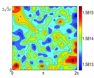
(a) t=0

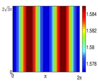
(b) t=160000

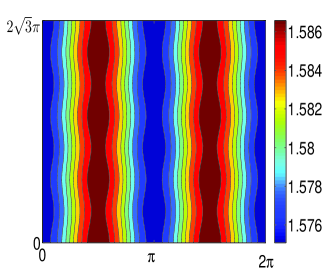
(c) t=200000

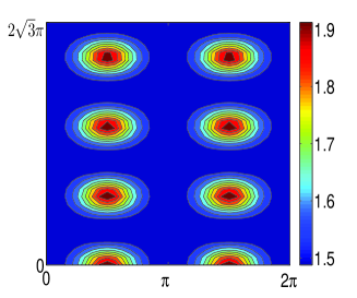
(d) t=240000

Figure 3.15: Cross-Roll instability. Starting from a random initial datum the solution evolves to the expected roll pattern (3.69). However a cross-roll instability leads to a mixed mode pattern.

A new set of rolls, corresponding to the mode $(0,7)$, grows perpendicularly to the original roll pattern. In the considered domain $L_{x}=2\pi$ and $L_{y}=2\sqrt{3}\pi$, the mode pair $(0,7)$ corresponds, in the sense of (2.18), to the eigenvalue $k_{m}^{2}=49/12\simeq 4.083$, which is nearly equal to the predicted most unstable eigenvalue $\bar{k}_{c}^{2}=4$. We shall interpret the formation of the cross-roll pattern as due to an intermode competition, following the approach presented in [41]. We perform the weakly nonlinear analysis and write the solution of the linear problem at $O(\varepsilon)$ as:

$${\bf w}_{1}=\mbox{\boldmath$\rho$}\left(A(T_{1},T_{2})\cos(2x)+B(T_{1},T_{2})\cos\left(\frac{7}{2\sqrt{3}}y\right)\right).$$ (3.70)

At $O(\varepsilon^{3})$ the following ODE model that illustrates the nonlinear behavior of the amplitudes $A$ and $B$ of the two competing modes $\bar{k}_{c}$ and $k_{m}$ is obtained:

$$\frac{dA}{dT_{2}} = \sigma_{1}A-L_{1}A^{3}+\Omega_{1}AB^{2},$$ (3.71a)

$$\frac{dB}{dT_{2}} = \sigma_{2}B-L_{2}B^{3}+\Omega_{2}A^{2}\,B,$$ (3.71b)

Here we skip all the details as the analysis of this system is similar to the case given in Section.3.2. For the considered set of parameters, the equilibria $(\pm A,0)$ and $(0,\pm B)$, each one corresponding to a roll pattern, are unstable. The unique stable states are $(\pm A,\pm B)$, as shown into the Fig.3.16, which corresponds to the cross-roll pattern.

The above method, however, does not explain the fact that the amplitude of the resulting pattern is $O(1)$ (see Fig.3.15(d)), which would probably require to consider also the competition with the hexagons modes and the spatial modulation of the pattern.

Figure 3.16: The phase plane of system (3.71). The competitive modes are $\bar{k}_{c}^{2}=4$ and $k_{m}^{2}=\frac{49}{12}$.

4 Conclusions

In this paper we have investigated the Turing mechanism induced by nonlinear cross-diffusion for two coupled reaction-diffusion equations on a two-dimensional spatial domain.

The possibility that the Turing bifurcation occurs via a degenerate eigenvalue makes the study mathematically involved, but gives rise to a rich variety of patterns which tessellate the plane and appear as steady state solutions of the reaction diffusion system. These are rolls, squares and mixed-mode patterns, among which there are the supersquares and the hexagons.

We have obtained the amplitude equations providing a mathematical description of the reaction-diffusion system close to the onset of instability. The analysis of the amplitude equations has shown the occurrence of a number of different phenomena, including stable subcritical Turing patterns or multiple branches of stable solutions leading to hysteresis. In particular, hexagonal patterns appear via a subcritical bifurcation and, from its same primary bifurcation point, rolls bifurcate supercritically. Therefore, there is a region of bistability where both rolls and hexagons are stable; however here rolls appear as a transient state due to a spatially modulated cross-roll instability that drives the solution toward a mixed modes pattern. Our attempt at explaining this instability as due to mode competition has been partially successful.

Future analysis might move from stationary Turing patterns to traveling patterning waves: when the domain size is large, the pattern is formed sequentially and traveling wavefronts are the precursors to patterning. In this case the equations governing the amplitude of the spatially modulated pattern (one has to consider the slow modulation in space of the pattern amplitude) will be the Ginzburg-Landau equation, or systems of Ginzburg-Landau equations in the degenerate case; we believe that these systems would be of independent and significant mathematical interest.

References

- [1] Y. Almirantis and S. Papageorgiou. Cross-diffusion effects on chemical and biological pattern formation. J. Theor. Biol., 151:289–311, 1991.
- [2] S. Aly and M. Farkas. Competition in patchy environment with cross diffusion. Nonlinear Analysis: Real World Applications, 5(4):589–595, 2004.
- [3] M. Andreianov, B. Bendahmane and R. Ruiz-Baier. Analysis of a finite volume method for a cross-diffusion model in population dynamics. Math. Mod. Meth. Appl. Sci., 21(2):307–344, 2011.
- [4] I. S. Aranson and L. S. Tsimring. Continuum theory of partially fluidized granular flows. Phys. Rev. E (3), 65(6):061303, 20, 2002.
- [5] J. W. Barrett and J. F. Blowey. Finite element approximation of a nonlinear cross-diffusion population model. Numer. Math., 98(2):195–221, 2004.
- [6] P. Becherer, A. N. Morozov, and W. van Saarloos. Probing a subcritical instability with an amplitude expansion: An exploration of how far one can get. Physica D, 238(18):1827–1840, 2009.
- [7] N. Ben Abdallah, P. Degond, and S. Genieys. An energy-transport model for semiconductors derived from the Boltzmann equation. J. Statist. Phys., 84(1-2):205–231, 1996.
- [8] S. Berres and R. Ruiz-Baier. A fully adaptive numerical approximation for a two-dimensional epidemic model with nonlinear cross-diffusion. Nonlinear Analysis: Real World Applications, 12:2888–2903, 2011.
- [9] L. Chen and A. Jüngel. Analysis of a multidimensional parabolic population model with strong cross-diffusion. SIAM J. Math. Anal., 36(1):301–322, 2004.
- [10] L. Chen and A. Jüngel. Analysis of a parabolic cross–diffusion population model without self–diffusion. J. Differential Equations, 224(1):39–59, 2006.
- [11] L. Chen and A. Jüngel. Analysis of a parabolic cross-diffusion semiconductor model with electron-hole scattering. Comm. Partial Differential Equations, 32(1-3):127–148, 2007.
- [12] R. Cherniha and L. Myroniuk. New exact solutions of a nonlinear cross-diffusion system. J. Phys. A: Math. Theor., 41(39):395204, 2008.
- [13] M. Cross and H. Greenside. Pattern Formation and Dynamics in Nonequilibrium Systems. Cambridge University Press, Cambridge, 2009.
- [14] M. C. Cross and P. C. Hohenberg. Pattern formation outside of equilibrium. Rev. Mod. Phys., 65, 1993.
- [15] G. C. Cruywagen, P. K. Maini, and J. D. Murray. Biological pattern formation on two-dimensional spatial domains: a nonlinear bifurcation analysis. SIAM J. Appl. Math., 57(6):1485–1509, 1997.
- [16] P. Degond, S. Génieys, and A. Jüngel. A system of parabolic equations in nonequilibrium thermodynamics including thermal and electrical effects. J. Math. Pures Appl. (9), 76(10):991–1015, 1997.
- [17] D. del Castillo-Negrete, B. A. Carreras, and V. Lynch. Front propagation and segregation in a reaction–diffusion model with cross-diffusion. Phys. D, 168/169:45–60, 2002.
- [18] B. Dionney, M. Silberz, and A. C. Skeldonx. Stability results for steady, spatially periodic planforms. Nonlinearity, 10, 1997.
- [19] J. M. Epstein. Nonlinear Dynamics, Mathematical Biology and Social Science. Addison-Wesley, Reading, MA, 1997.
- [20] J.N. Flavin and S. Rionero. Cross-diffusion influence on the nonlinear stability analysis. IMA J. Appl. Math., 72(5), 2007.
- [21] G. Galiano. On a cross-diffusion population model deduced from mutation and splitting of a single species. Computers & Mathematics with Applications, 64(6):1927 – 1936, 2012.
- [22] G. Galiano, M. L. Garzón, and A. Jüngel. Semi-discretization in time and numerical convergence of solutions of a nonlinear cross-diffusion population model. Numer. Math., 93(4):655–673, 2003.
- [23] G. Galiano, A. Jüngel, and J. Velasco. A parabolic cross-diffusion system for granular materials. SIAM J. Math. Anal., 35(3):561–578 (electronic), 2003.
- [24] G. Galiano and J. Velasco. Competing through altering the environment: A cross-diffusion population model coupled to transport–darcy flow equations. Nonlinear Analysis: Real World Applications, 12(5):2826–2838, 2011.
- [25] G. Gambino, M. C. Lombardo, and M. Sammartino. A velocity-diffusion method for a Lotka-Volterra system with nonlinear cross and self-diffusion. Appl. Numer. Math., 59(5):1059–1074, 2009.
- [26] G. Gambino, M. C. Lombardo, and M. Sammartino. Turing instability and traveling fronts for a nonlinear reaction–diffusion system with cross-diffusion. Mathematics and Computers in Simulation, 82(6), 2012.
- [27] E. Gilad, J. von Hardenberg, A. Provenzale, M. Shachak, and E. Meron. A mathematical model of plants as ecosystem engineers. J. Theoret. Biol., 244(4):680–691, 2007.
- [28] M. van Hecke, P.C. Hohenberg, and W. van Saarloos. Amplitude equations for pattern forming systems. In H. van Beijeren and M.H. Ernst, editors, Fundamental Problems in Statistical Mechanics VIII, pages 245–278, Amsterdam, 1994. North-Holland.
- [29] R. Hoyle. Pattern Formation. An Introduction to Methods. Cambridge University Press, Cambridge, 2006.
- [30] A. Jüngel. Diffusive and nondiffusive population models. In Mathematical modeling of collective behavior in socio-economic and life sciences, Model. Simul. Sci. Eng. Technol., pages 397–425. Birkhäuser Boston Inc., Boston, MA, 2010.
- [31] D. Lauffenburger, R. Aris, and K. Keller. Effects of cell motility and chemotaxis on microbial population growth. Biophys. J., 40:209–219, 1982.
- [32] Y. Lou and W. M. Ni. Diffusion, self-diffusion and cross-diffusion. J. Differential Equations, 131(1):79–131, 1996.
- [33] P. K. Maini and J. D. Murray. A nonlinear analysis of a mechanochemical model for biological pattern formation. SIAM J. Appl. Math., 48:1064–1072, 1988.
- [34] P. Manneville. Instabilities, Chaos, and Turbulence. Imperial College Press, London, 2004.
- [35] M. Mimura and K. Kawasaki. Spatial segregation in competitive interaction–diffusion equations. J. Math. Biol., 9(1):49–64, 1980.
- [36] G. Mulone, S. Rionero, and W. Wang. The effect of density-dependent dispersal on the stability of populations. Nonlinear Anal., 74(14):4831–4846, 2011.
- [37] A. Newell and J. Whitehead. Finite band width, finite amplitude convection. J. Fluid. Mech, 38:279–303, 1969.
- [38] G. A. Ngwa and P. K. Maini. Spatio-temporal patterns in a mechanical model for mesenchymal morphogenesis. J. Math. Biol., 33:489–520, 1995.
- [39] W.H. Ruan. Positive steady-state solutions of a competing reaction–diffusion system with large cross-diffusion coefficients. J. Math. Anal. App., 197(2):558–578, 1996.
- [40] Ricardo Ruiz-Baier and Canrong Tian. Mathematical analysis and numerical simulation of pattern formation under cross-diffusion. Nonlinear Analysis: Real World Applications, 14(1):601 – 612, 2013.
- [41] L. A. Segel. The non-linear interaction of two disturbances in the thermal convection problem. J. Fluid Mech., 14:97–114, 1962.
- [42] J. A. Sherratt. Wavefront propagation in a competition equation with a new motility term modelling contact inhibition between cell populations. R. Soc. Lond. Proc. Ser. A Math. Phys. Eng. Sci., 456(2002):2365–2386, 2000.
- [43] N. Shigesada, K. Kawasaki, and E. Teramoto. Spatial segregation of interacting species. J. Theo. Biology, 79:83–99, 1979.
- [44] C. Tian, Z. Lin, and M. Pedersen. Instability induced by cross-diffusion in reaction–diffusion systems. Nonlinear Analysis: Real World Applications, 11:1036–1045, 2010.
- [45] A. M. Turing. The chemical basis of morphogenesis. Phil. Trans. Roy. Soc. London, B, 237:37–72, 1952.
- [46] V.K. Vanag and I.R. Epstein. Cross-diffusion and pattern formation in reaction–diffusion system. Phys. Chem. Chem. Phys., 11:897 – 912, 2009.
- [47] Z. Wen and S. Fu. Global solutions to a class of multi-species reaction–diffusion systems with cross-diffusions arising in population dynamics. J. Comput. Appl. Math., 230(1):34–43, 2009.
- [48] D. J. Wollkind, V.S. Manoranjan, and L. Zhang. Weakly nonlinear stability analyses of prototype reaction–diffusion model equations. SIAM Rev., 36(2):176–214, 1994.
- [49] Y. Wu and X. Zhao. The existence and stability of travelling waves with transition layers for some singular cross-diffusion systems. Physica D, 200:325–358, 2005.
- [50] H. Yizhaq, B.A. Portnov, and E. Meron. A mathematical model of segregation patterns in residential neighbourhoods. Environment and Planning A, 36:149 – 172, 2004.
- [51] J.F. Zhang, W.T. Li, and Y.X. Wang. Turing patterns of a strongly coupled predator-prey system with diffusion effects. Nonlinear Analysis: Theory, Methods & Applications, 74:847 – 858, 2011.