HerMES: Unveiling obscured star formation – the far infrared luminosity function of ultraviolet-selected galaxies at $\boldsymbol{z\sim 1.5}$

Abstract

We study the far-infrared (IR) and sub-millimeter properties of a sample of ultraviolet (UV) selected galaxies at $z\sim 1.5$. Using stacking at 250, 350 and 500 $\mu$m from Herschel Space Observatory SPIRE imaging of the COSMOS field obtained within the HerMES key program, we derive the mean IR luminosity as a function of both UV luminosity and slope of the UV continuum $\beta$. The IR to UV luminosity ratio is roughly constant over most of the UV luminosity range we explore. We also find that the IR to UV luminosity ratio is correlated with $\beta$. We observe a correlation that underestimates the correlation derived from low-redshift starburst galaxies, but is in good agreement with the correlation derived from local normal star-forming galaxies. Using these results we reconstruct the IR luminosity function of our UV-selected sample. This luminosity function recovers the IR luminosity functions measured from IR selected samples at the faintest luminosities ($L_{\rm{IR}}\sim 10^{11}\,{\rm L}_{\sun}$), but might underestimate them at the bright-end ($L_{\rm{IR}}\ga 5\times 10^{11}\,{\rm L}_{\sun}$). For galaxies with $10^{11}<L_{\rm{IR}}/{\rm L}_{\sun}<10^{13}$, the IR luminosity function of a UV selection recovers (given the differences in IR-based estimates) 52-65 to 89-112 per cent of the star-formation rate density derived from an IR selection. The cosmic star-formation rate density derived from this IR luminosity function is 61-76 to 100-133 per cent of the density derived from IR selections at the same epoch. Assuming the latest Herschel results and conservative stacking measurements, we use a toy model to fully reproduce the far IR luminosity function from our UV selection at $z\sim 1.5$. This suggests that a sample around 4 magnitudes deeper (i.e. reaching $u^{*}\sim 30$  mag) and a large dispersion of the IR to UV luminosity ratio are required.

1 Introduction

Star-formation is one of the main properties used to trace galaxy formation and evolution. Our ability to constrain the mechanisms that drive galaxy evolution hence depends to a large extent on our ability to measure accurate star-formation rates for samples of galaxies. A number of star-formation tracers are routinely used, from the strengths of spectral lines to broad-band measurements (Kennicutt, 1998). Broad-band measurements offer the advantage that estimates can be derived for a large number of galaxies with minimal spectroscopic follow-up, albeit at the expense of possible contamination by strong spectral features (e.g. Smail et al., 2011). One of the main star-formation rate tracers of this kind comes from the ultraviolet (UV) range of the spectrum, where most of the energy is emitted by young stars (ages $\sim 10^{7}{-}10^{8}$ Myr; see e.g. Martin et al., 2005a). The UV has been widely used over a large redshift range to infer the cosmic star-formation density, from $z=7$ to $z=0$ (e.g. Schiminovich et al., 2005; Bouwens et al., 2009).

Optical/near infrared (IR) observations probe the rest-frame UV for samples of galaxies at high redshift, hence it has been the primary choice for constraining the star-formation activity of the Universe at early epochs from large samples. However, interstellar dust, which is a byproduct of star-formation, makes the measurement of star-formation activity challenging at these wavelengths. Dust grains scatter or absorb the light emitted by young stars; hence only a fraction of the energy output from star-formation is observable in the UV. Dust grains re-emit this energy over the full IR range $8-1000\,\mu$m. One way to estimate the dust attenuation in the UV and to assess the selection bias inherent to the UV is then to study the far IR properties of UV-selected galaxies.

A number of studies have used this approach to characterise the amount of dust attenuation. In the local Universe, the star-formation rate density is roughly equally divided between UV and IR contributions (Martin et al., 2005b; Bothwell et al., 2011). At earlier epochs, however, the fraction of star-formation rate density, which is directly measurable using the UV continuum, decreases from 44 per cent ($z=0$) to roughly 15 per cent at $z\sim 1$ (Takeuchi, Buat, & Burgarella, 2005; Tresse et al., 2007), while it might increase slightly to 20 per cent at $2<z<3.5$ (Reddy et al., 2008), and even to higher values in the early Universe (Bouwens et al., 2010).

To overcome this drawback and the lack of deep IR data, it is common to use empirical recipes to correct UV for dust attenuation. The most well-known is the relation between the slope of the UV continuum and the ratio of the luminosities in the IR and the UV (Meurer, Heckman, & Calzetti, 1999). The slope of the UV continuum can be derived from rest-frame UV colours, and hence is convenient for estimating star formation rates at high redshifts when a limited wavelength range is available (Schiminovich et al., 2005; Bouwens et al., 2009).

However, this recipe does encounter several pitfalls: it has been derived from local starburst galaxies, and it might not be valid for more normal star-forming galaxies (Boissier et al., 2007; Cortese et al., 2006; Muñoz-Mateos et al., 2009; Hao et al., 2011). Moreover, the relation between dust attenuation and UV slope depends on the selection criteria (Buat et al., 2005; Seibert et al., 2005), and might also be sensitive to star-formation history (Kong et al., 2004; Panuzzo et al., 2007), as well as dust properties (Inoue et al., 2006) and dust geometry (Calzetti, 2001).

It is hence of particular importance to follow the evolution with redshift of the IR properties of UV-selected galaxies, in order to characterize the biases inherent in such selection, and also to examine the validity of the empirical recipes commonly used to correct for dust attenuation.

In this context a new era started with the availability of data from the Herschel telescope (Pilbratt et al., 2010). Indeed, while Spitzer data uncovered the dusty star-formation history of the Universe up to $z\simeq 1$ (Le Floc’h et al., 2005), at higher redshifts large extrapolations are needed to estimate IR luminosities from 24$\,\mu$m data, which could lead to systematic errors (Bavouzet et al., 2008a), as they do not probe the peak of the dust emission. Based on Herschel data, Elbaz et al. (2010) showed, for instance, that using mid-IR data at $z>1.5$ leads to an overestimation of the total IR luminosity. Another important feature of the submillimeter wavelength range is that the contribution of Active Galactic Nuclei to the galaxy Spectral Energy Distribution (SED) is generally outweighed by the star-formation component for $\lambda\ga$ 30 $\mu$m (Hatziminaoglou et al., 2010).

In this paper, we focus on a UV-selected sample at $z\sim 1.5$ to study with unprecedented statistics the far IR properties of UV-selected galaxies using Herschel data for more accurate measurements of IR luminosities. Given the confusion-limited nature of these data, we rely on a stacking analysis to derive the mean IR luminosities for different classes of object (e.g. Béthermin et al., 2012; Hilton et al., 2012; Viero et al., 2012b).

The paper is organized as follows. We start by presenting the sample construction and the need for stacking (Section. 2). In Section 3 we present our methods for stacking measurements and corrections for biases. Section 4.1 shows our stacking results as a function of UV luminosity and Section 4.2 as a function of the slope of the UV continuum. In Section 5 we reconstruct the total IR luminosity function of our UV-selected sample using the stacking results, and examine the implications of these results for the measurement of the cosmic star-formation density from UV and IR selected samples. We discuss these results in Section 6 and present our conclusions in Section 7.

In this paper, we use a standard cosmology with $\Omega_{\rm m}=0.3$, $\Omega_{\Lambda}=0.7$ and $H_{0}=70$ km s^-1Mpc^-1, denote FUV and IR luminosities as $\nu L_{\nu}$, and use AB magnitudes.

2 Data sample

We use optical imaging of the COSMOS field from Capak et al. (2007) in the $u^{\ast}$-band (obtained at CFHT; depth: 26.4 mag at 5$\sigma$ for a 3 arcsec aperture) and $V_{J}$-band (from Subaru; depth: 26.6 mag, also at 5$\sigma$ for a 3 arcsec aperture). We generated catalogues from the $u^{\ast}$ and $V_{J}$ images using SExtractor (Bertin & Arnouts, 1996) in order to select galaxies directly in the $u^{*}$-band, and obtain accurate total fluxes. Comparison with the photometry from Capak et al. (2007) shows good agreement. Hereafter all quoted magnitudes are corrected for Galactic extinction using dust maps from Schlegel, Finkbeiner, & Davis (1998).

We estimated the incompleteness by injecting 1000 fake sources in the $u^{\ast}$ image with random positions. We injected sources only within areas not masked for edges or bright stars. We assumed that the objects in our UV-selected sample are pure exponential disks. We assumed that the disk scale length for galaxies with $L_{\textrm{FUV}}=L^{*}\sim 10^{10}\rm{L}_{\odot}$ is equal to 3 kpc. This value is 50 per cent larger than the one from Fathi et al. (2012), determined at $0.3<z<2.0$ in the $z$-band (restframe wavelength 4600 Å at $z=1$), in order to account for the fact that disks are larger at UV wavelengths. The value we assumed is in agreement with predictions from Boissier & Prantzos (2001), as well as with the UV restframe measurements from Ferguson et al. (2004), taking into account that the mean luminosity of their sample is around $5\times L^{*}_{\textrm{FUV}}(z=1.5)$. We further assumed that the disk scale length varies with luminosity as $L^{1/3}$, as observed in the local Universe (de Jong & Lacey, 2000). We generated fake objects following the observed joint distributions of magnitude, redshift, and minor to major axis ratio; we also allowed random position angles. Then for each fake object we could infer its UV luminosity and its disk scale length. We injected these objects in the $u^{\ast}$ image after convolving them with the $u^{\ast}$-band PSF (FWHM = $0.9$ arcsec, Capak et al., 2007). We performed source extraction with SExtractor on this new image using the same parameters as the ones used to generate the $u^{\ast}$-band catalogue, but using this time the ASSOC mode to cross-match directly the detections with our input fake sources list, with a 0.5 arcsec search radius. We performed this process 1500 times to have sufficient statistics to quantify the effects of incompleteness on stacking (see Sect. 3.1). In order to test the impact of real sources on the flux estimation of the fake sources, we cross-matched the fake sources we recovered with the full $u^{*}$-band catalog. We then rejected fake sources whose magnitudes are perturbed by closeby real sources, based on the angular separation and the difference between the input and the recovered magnitude.

We estimate that the completeness is $76\pm 1$ per cent at the limiting magnitude $u^{\ast}=26$ mag (Fig. 1).

We cross-matched our sample with an updated version of the photometric redshift catalogue of Ilbert et al. (2009, v.2.0). This version differs from the original Ilbert et al. (2009) catalogue by the inclusion of additional near-IR photometry (YJHK, McCracken et al., 2012) which improves the accuracy of the photometric redshifts, in particular in the redshift range we are interested in. 98.5 per cent of the sources from our sample have a counterpart in the Ilbert et al. (2009) catalogue within a 1 arcsec search radius.

We built a rest-frame UV-selected catalogue considering objects with $1.2<z_{\rm phot}<1.7$ and $u^{\ast}<26$ mag. The average photometric redshift accuracy at $1\sigma$ in $(1+z)$ is 0.04 for this sample, and the mean redshift is $\langle z_{\rm phot}\rangle=1.43$. At this redshift, the effective wavelength of the $u^{*}$-band filter corresponds to 1609 Å, which is in the far-UV (FUV) rest-frame. Our final catalogue contains 42,184 objects over 1.68 deg², after masking of edges and areas around bright stars.

Figure 1: Completeness in the $u^{*}$ band for the UV-selected catalogue. Error bars are the errors on the mean. The vertical dashed line shows the magnitude limit we adopt.

We use Herschel-SPIRE (Griffin et al., 2010; Swinyard et al., 2010) imaging at 250 (FWHM $=18.15$ arcsec), 350 (FWHM $=25.15$ arcsec), and 500 $\mu$m (FWHM $=36.3$ arcsec) of the COSMOS field obtained as part of the Herschel Multi-Tiered Extragalactic Survey (HerMES, Oliver et al., 2012) programme. We use here the images produced by the SMAP pipeline (Levenson et al., 2010; Viero et al., 2012a). The effective area (after removing masked regions) of the overlap between $u^{\ast}$-band and Herschel-SPIRE images is 1.5 deg²; 38,074 galaxies from our UV-selected catalogue are within this area.

We performed cross-matching between our UV-selected catalogue and the SCAT (Smith et al., 2012) blind detections at 250, 350 and 500 $\mu$m, using a 5 arcsec search radius. Considering as ‘detected’ only Herschel-SPIRE sources with fluxes larger than the confusion limit (at 5$\sigma$, 24.0 mJy at 250 $\mu$m, 27.5 mJy at 350 $\mu$m, and 30.5 mJy at 500 $\mu$m, Nguyen et al., 2010), we find that less than 1 per cent of the UV sources are detected at 250, 350, and 500 $\mu$m. This result implies that we need to use a stacking analysis in order to study in a statistical way the IR properties of the UV-selected galaxies in our sample. In the following, we include all UV-selected galaxies within the HerMES footprint in the stacking analysis, whether they are detected at the Herschel-SPIRE wavelengths or not. Excluding UV-selected galaxies detected at SPIRE wavelengths from the stacking input lists does not significantly impact our results.

We further use this sample of UV-selected galaxies detected at SPIRE wavelengths to determine the dispersion in $L_{\rm IR}/L_{\rm FUV}$ as a function of $L_{\rm FUV}$. This sample has a mean infrared luminosity $\langle L_{\rm IR}\rangle=10^{12}\rm{L}_{\odot}$, is slightly brighter in UV than our full sample ($\langle L_{\rm FUV}\rangle=2.6\times 10^{10}\rm{L}_{\odot}$, compared to $10^{10}\rm{L}_{\odot}$ for the full sample), and has a mean IR to UV luminosity ratio of $\langle L_{\rm IR}/L_{\rm FUV}\rangle=66$.

3 Stacking measurements

We use the IAS library (Bavouzet, 2008b; Béthermin et al., 2010a) to perform the stacking. We use the calibrated 250, 350 and 500 $\mu$m images, and we do not attempt to clean the image of any detected sources at SPIRE wavelengths.

For a given stacking measurement, we generate both a postage stamp image and a radial profile, using the mean of the individual images that are included in the stacking. We derive errors on the profiles by bootstrap resampling.

The background for the stack images is usually considered constant and determined by the average value of the stack profile at large distances from the centre of the stack image. However, a number of effects can yield a non homogeneous background; we correct our stacking measures for two effects which have an impact on the background: the incompleteness of the input catalogue, and the clustering of the input galaxies. These corrections are based on the work of Bavouzet (2008b) and Béthermin et al. (2010b).

3.1 Correcting for stacking bias

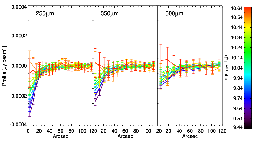
Figure 2: Profiles of the stacking at 250, 350 and 500 $\mu$m of recovered fake sources in bins of $L_{\rm FUV}$ luminosity.

While limited, the incompleteness at the faint-end of the input catalogue can have an impact on the stacking measurements, for instance if it is partly related to the local geometry during the detection process. In particular, the detection efficiency for faint objects is lower in dense areas of the image. As we will see, this effect can also be described by a clustering term under the form of a cross correlation between sources of different $u^{*}$ band fluxes.

If we stack a population of objects which is randomly distributed in the sky, we will get a flat background. On the other hand, if there is a bias introduced by the detection process, we will miss the contribution of the objects which are not recovered by the source extraction. The basis of this correction is to measure the actual background of the stacking for a given class of input sources.

We assume here that the stacking bias effects are related to the UV luminosity of the objects. In other words, we consider the actual $L_{\rm FUV}$ distribution for each class of galaxy to correct for this bias. To quantify the impact of the stacking bias, we use the fake sources created to estimate the completeness of our catalogue (see Sect. 2). We stack the fake sources recovered by the detection process with the same UV luminosity distribution as the class of galaxy we are considering. We show in Fig. 2 the radial profiles of the stacking as a function of $L_{\rm FUV}$. These profiles are based on a sample of fake sources with roughly 25 times the actual number of galaxies in our sample. The error bars on these profiles are obtained through bootstrap resampling. For faint objects ($L_{\rm FUV}<10^{10}\,{\rm L}_{\sun}$), at smaller scales, the profiles are actually lower than zero. Note that the amplitude of this effect increases for fainter objects.

This result is related to the well-known effect that the detection efficiency is lower in dense areas, and in particular for faint objects which are close to brighter ones. If all fake sources were to be recovered by the UV source extraction, the profile of their stacking at the Herschel-SPIRE wavelength would be zero, as their input distribution is independent of that of the real sources. However, the faint sources which are close to bright real sources in the $u^{*}$ image are not completely recovered. This effect is more important for fainter sources, as well as for smaller distances with respect to bright sources. Hence, the stacking of faint objects is missing the contribution to the background of the ones which happen to be closer to UV-bright sources, and then the background at small scales is lower.

In order to correct our stacking measurement for this effect, we subtract these profiles, without smoothing, from the profiles of the stacked images. We add in quadrature the errors of these profiles to the errors of the stacked image profiles.

We show as squares in Fig. 3 the ratio of the flux densities corrected from the stacking bias to the flux densities measured with PSF-fitting, assuming a constant background, as a function of $L_{\rm FUV}$. The amplitude of the correction is maximal at faint luminosities (around 2 times the flux from direct PSF-fitting at $L_{\rm FUV}\sim 6\times 10^{9}\,{\rm L}_{\sun}$) then decreases with luminosity, to be negligible for $L_{\rm FUV}\ga 2\times 10^{10}\,{\rm L}_{\sun}$.

3.2 Correcting for clustering of the input catalogue

We use the formalism developped by Bavouzet (2008b) and Béthermin et al. (2010b) in order to take into account the impact on the measured flux from the clustering of the population under study. If the input population is uniformly distributed on the sky, the measured stacking is just the average flux of the population at the stacked wavelength. In practice, galaxies are clustered, so there is an excess of probability to find another galaxy of the sample within the beam, compared to the value derived from a randomly distributed population. This yields an overestimation of the flux. The probability is proportional to the angular correlation function of the class of galaxies under study. The two dimensional profile of the resulting stacking can then be written as:

$$I(\theta,\phi)=\overline{S}\times\textrm{PSF}(\theta,\phi)+a\times\big{[}w(\theta,\phi)\ast\textrm{PSF}(\theta,\phi)\big{]}\textrm{.}$$ (1)

Here $\overline{S}$ is the average flux, PSF$(\theta,\phi)$ is the Point Spread Function at the stacked wavelength, $w(\theta,\phi)$ is the angular autocorrelation function of the input population; the symbol $\ast$ denotes a convolution, and $a$ is a parameter relating to the density of the input population and their contribution to the cosmic background. The effect of the clustering is to add to the profile a component which is broader than the pure PSF (see e.g. Béthermin et al., 2012, their fig. 3).

To correct our stacking measures for clustering, we adjust the radial profile of each stacked image over 120 arcsec following eq. 1, with $\overline{S}$ and $a$ as free parameters, and using the autocorrelation function $w(\theta)$ of the sample. We obtain the best value of $\overline{S}$ by marginalising the two dimensional probability of $(\overline{S},a)$ over $a$, using $\chi^{2}$ statistics.

In this paper we perform stacking in bins of UV luminosity and the slope of the UV continuum ($\beta$). We measure $w(\theta)$ using the method of Szapudi et al. (2005), and fit it with a power law $w(\theta)=A_{w}\theta^{-\delta}$, correcting for the integral constraint following Roche & Eales (1999). We find that the correlation function is well modelled with $\delta=0.64\pm 0.07$. Note that we consider $a$ as a free parameter in eq. 1, so our results do not depend on the actual value of $A_{w}$.

The angular correlation function depends on UV luminosity (see e.g. Giavalisco & Dickinson, 2001; Heinis et al., 2007; Savoy et al., 2011), while there is no evidence that it depends on $\beta$. We checked that while there are some variations in amplitude and slope of the correlation function with UV luminosity, they are not sufficient in this context to significantly change the correction for the flux determination. We consider only the best fit to the correlation function from the full sample hereafter.

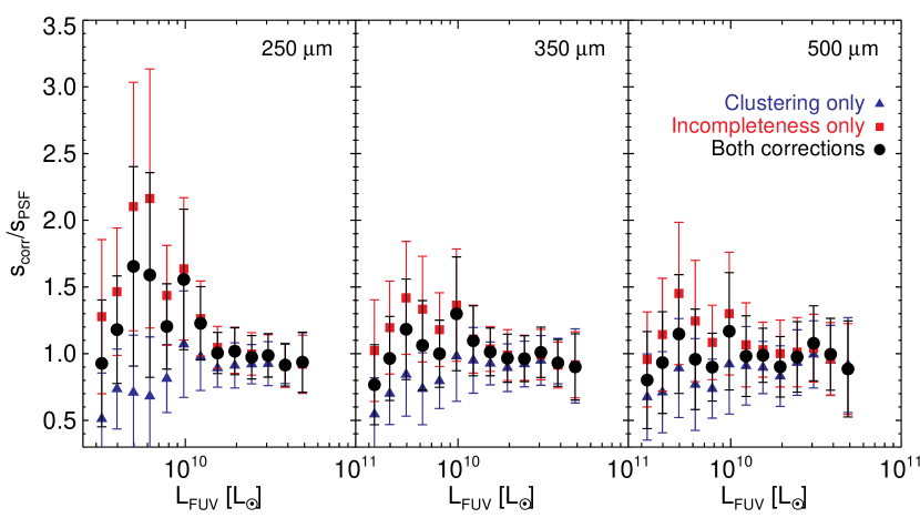
Figure 3: Amplitude of the correction applied to stacked flux densities as a function of $L_{\rm FUV}$, at 250, 350 and 500 $\mu$m. We show here the ratio of the corrected stacked flux density to the flux density measured by a simple PSF-fitting. The triangles show this ratio for the correction due to the clustering of the input catalogue, the squares are the correction applied because of the incompleteness of the input catalogue, and the circles show the ratio for the total correction including clustering and incompleteness.

We show as triangles on Fig. 3 the ratio of the flux densities corrected from clustering to the flux densities measured with PSF-fitting, as a function of $L_{\rm FUV}$. The amplitude of the correction is blue around $-20$ per cent compared to the PSF-estimated flux at $L_{\rm FUV}<10^{10}L_{\odot}$, and becomes negligible for $L_{\rm FUV}>10^{10}L_{\odot}$. The amplitude of this correction is larger for the faint bins, where we observe a stronger departure from a PSF profile (see Appendix B).

3.3 Summary: flux density measurements

For a given stacking measure, we correct first for stacking bias by subtracting the stacking bias profile from the stack profile, adding errors of the profiles in quadrature. The stacking bias profile used is derived by stacking fake sources recovered by source extraction using the same $L_{\rm FUV}$ distribution as the galaxies in the stack under study. We then fit the resulting profile with eq. (1), leaving $\overline{S}$ and $a$ as free parameters, in order to get a flux density corrected from the effect of clustering. We show in Fig. 3 the amplitude of the correction (combining effects of incompleteness and clustering as circles) as a function of $L_{\rm FUV}$. These corrections partly compensate for each other; the amplitude of the overall correction decreases with luminosity. The correction is maximal at $L_{\rm FUV}=6\times 10^{9}\,{\rm L}_{\sun}$ and becomes negligible for luminosities larger than $2\times 10^{10}\,{\rm L}_{\sun}$. The overall correction is larger at faint luminosities because the incompleteness is more important, and also because of the larger departure of the observed profiles from a pure PSF. Note that the errors on Fig. 3 are large for faint luminosities because the errors on $S_{\rm{PSF}}$ are large (around twice the errors on $S_{\rm{corr}}$); the amplitude of the correction itself is well determined.

The errors on the flux density $\overline{S}$ are obtained by boostrap resampling, repeating the above procedure on 3000 random bootstrap samples, and determining the error from the standard deviation of the fluxes of these bootstrap samples.

We further performed the following tests to assess the reliability of our results. First of all, we performed the full analysis using median stacking, and obtained very similar results (see Appendix C.1). We also tested how detected objects impact our stacking results. We subtracted from the SPIRE images the sources detected at various threshold levels (from 3 to 10$\sigma$). We performed the stacking on these images, and added to the flux measured by stacking the flux of the detected objects. The results we obtain with this method are slightly higher (on average 20 per cent, see Appendix C.2) than the results presented here, while they agree at the 1$\sigma$ level. The results do not depend significantly on the threshold level we use to subtract detected objects. We discuss in Sect. 5.3 the impact of this difference on the cosmic star formation rate density derived from the IR luminosity functions we build from the stacking measurements.

4 Results

We perform stacking at 250, 350, and 500 $\mu$m as a function of UV luminosity and slope of the UV continuum, $\beta$. Tables with stacking results are in Appendix A, and we show the postage stamp images of the stacking in Appendix B. We derive total IR luminosity, $L_{\rm{IR}}$, by integrating over the range $8<\lambda<1000\,\mu$m of the best fit to the Dale & Helou (2002) templates, obtained with the SED-fitting code CIGALE (Noll et al., 2009). There are various ways to assign a redshift to a given stack population; we consider here as the redshift the mean photometric redshift of the galaxies involved in the stacking. The error on $L_{\rm{IR}}$ is given by the standard deviation of the probability distribution function of the $L_{\rm IR}$ values obtained with the models used during the fitting procedure (see Noll et al., 2009).

The Dale & Helou (2002) templates are calibrated as a function of a single parameter $\alpha$. These models assume that the dust mass over interstellar radiation field ratio varies as a power law of the interstellar radiation field with index $-\alpha$. We observe slight variations of this parameter as measured by the SED fitting. As a function of luminosity, we find that $\alpha$ decreases from $\sim 2.6$ for $L_{\rm FUV}<1.5\times 10^{10}\,{\rm L}_{\sun}$ to $\sim 1.7$ for $L_{\rm FUV}>1.5\times 10^{10}\,{\rm L}_{\sun}$, which implies an increase of dust temperature from $\sim$ 25 to 30 K. The significance of this increase is however only at a level of 1.1$\sigma$. As a function of the slope of the UV continuum, $\beta$, $\alpha$ is roughly constant at around $1.8$, which implies a dust temperature of around 28 K.

4.1 Stacking as a function of UV luminosity

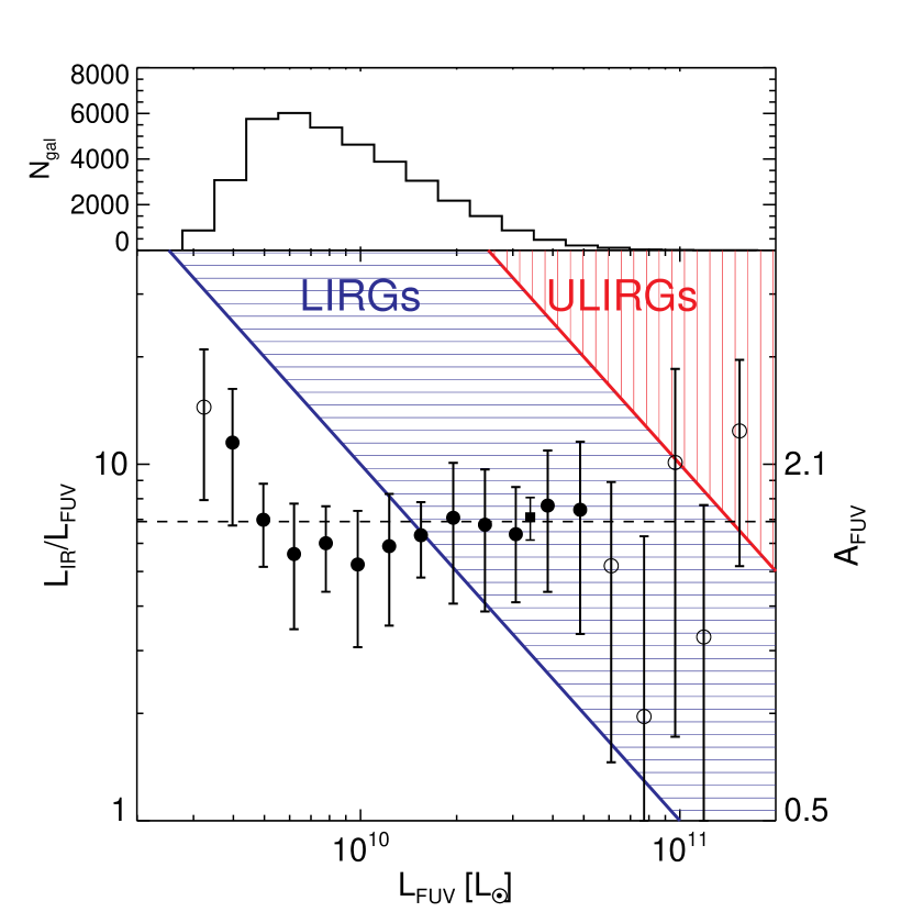
Figure 4: IR-to-UV luminosity ratio as a function of UV luminosity. Estimates with $S/N>3$ at 250, 350 and 500 $\mu$m are shown as filled circles, and others as empty circles. The horizontally hatched region represents the locus of LIRGs, while the vertically hatched region is for ULIRGs. The dashed line shows the mean $L_{\rm IR}/L_{\rm FUV}$ value from estimates with $S/N>3$ at 250, 350 and 500 $\mu$m. The filled square shows the estimate from stacking of UV-selected galaxies at Herschel-PACS wavelengths at $z\sim 2$ of Reddy et al. (2012), slightly offset in $L_{\rm FUV}$ for clarity. The right axis shows the equivalent attenuation in the FUV band (in magnitudes), using eq. 2. The top panel shows the histogram of galaxies as a function of $L_{\rm FUV}$.

We stack UV-selected galaxies in bins of UV luminosity $L_{\rm FUV}$ of size 0.1 dex. The results are presented in Fig. 4, where we plot the ratio of IR to UV luminosities (which is a tracer of dust attenuation) as a function of the UV luminosity. The $L_{\rm{IR}}/L_{\rm FUV}$ ratio is found to be constant with UV luminosity over most of the range we probe, with a mean of $6.9\pm 1.$ This suggests that the dust attenuation does not depend heavily on UV luminosity in a UV-selected sample at $z\sim 1.5$ in this luminosity range. Assuming that the relation between the attenuation in the GALEX FUV band and $L_{\rm{IR}}/L_{\rm FUV}$ is (Overzier et al., 2011; Seibert et al., 2005)

$$A_{\rm FUV}=2.5\log\left[\frac{1}{1.68}\left(\frac{L_{\rm{IR}}}{L_{\rm FUV}}\right)+1\right],$$ (2)

the average value of the IR to UV luminosity ratio for our sample corresponds to a value $A_{\rm FUV}=1.8\pm 0.1$ mag.

We also show in Fig. 4 the regions where Luminous Infrared Galaxies (LIRGs, $10^{11}<L_{\rm{IR}}/{\rm L}_{\sun}<10^{12}$) and Ultra Luminous Infrared Galaxies (ULIRGs, $L_{\rm{IR}}>10^{12}\,{\rm L}_{\sun}$) lie. Our results show that the average IR luminosities of UV-selected galaxies in the UV luminosity range we explore at $z\sim 1.5$ are comparable to LIRGs, but not to ULIRGs. Our measures of the $L_{\rm{IR}}/L_{\rm FUV}$ ratio are in agreement with previous measures obtained from objects within UV-selected samples detected in both the UV and IR (Reddy et al., 2006b; Buat et al., 2009; Reddy et al., 2010). Our result is also in excellent agreement with the stacking study of Reddy et al. (2012), who found that the average IR-to-UV luminosity ratio of a sample of 114 UV-selected galaxies at $z\sim 2$ is $7.1\pm 1.1$, for galaxies with $L_{\rm FUV}\sim 3.1\times 10^{10}\,{\rm L}_{\sun}$. Note also that Buat et al. (2009) observed that the fraction of galaxies with $L_{\rm{IR}}/L_{\rm FUV}>5$ is roughly constant with UV luminosity for $L_{\rm UV}\ga 3\times 10^{9}\,{\rm L}_{\sun}$, which is consistent with the trend we measure here. We can also compare our result with the average attenuation derived by Cucciati et al. (2012) from SED fitting of galaxies selected in the $I$-band (around 3000 Å rest-frame at the mean redshift of our sample) with $u^{*}g^{\prime}r^{\prime}i^{\prime}zJHK_{\rm s}$ photometry and spectroscopic redshifts. They derive $A_{\rm FUV}=2.17$ mag for the same redshift range ($1.2<z<1.7$) as our study, which is slightly larger than what we measure, though note that we select galaxies at shorter restframe wavelengths.

4.2 Stacking as a function of UV slope, $\beta$

The slope of the UV continuum has been shown to correlate with the dust attenuation within galaxies (e.g. Calzetti, Kinney, & Storchi-Bergmann, 1994; Meurer, Heckman, & Calzetti, 1999). The use of the $\beta$ slope offers an estimate of the dust attenuation from the rest-frame UV, without requiring far-IR data or spectral lines diagnostics. Calibrations have been derived from spectro-photometric samples of starburst galaxies at low redshifts (e.g. Meurer, Heckman, & Calzetti, 1999; Overzier et al., 2011), and are routinely used to derive dust attenuation at various redshifts, in particular using slopes derived from rest-frame UV colours.

We use the $u^{*}$, $V$, intermediate (IA427, IA464, IA484, IA505, IA527, IA574, IA624, IA679, IA709, IA738, IA767, IA827) and narrow-band (NB711, NB816) filters to compute the slope $\beta$. We adjust the photometry to a simple power-law SED, $f_{\lambda}\propto\lambda^{\beta}$, over the restframe wavelength range $1200<\lambda<3000$ Å. This means that there are at least 9 bands available for the measure of $\beta$, and at the mean redshift of this sample, $z=1.43$, there are 12 bands available.

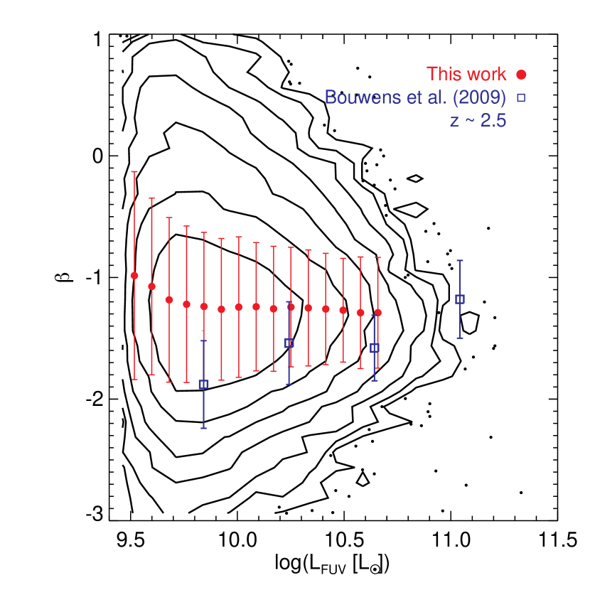
Figure 5: UV continuum slope $\beta$ as a function of UV luminosity. The large filled circles show the mean and dispersion in 15 bins of luminosity for $L_{\rm FUV}<5\times 10^{10}\,{\rm L}_{\sun}$. Open squares show the mean $\beta$ measured for $U$-band dropouts from WFPC2 (F300W) data at $z\sim 2.5$ (Bouwens et al., 2009).

Figure 5 shows the distribution of $\beta$ as a function of UV luminosity. The mean UV slope for our sample is $\langle\beta\rangle=-1.2\pm 0.6$. We find that the average slope of the UV continuum is mostly independent of the UV luminosity, while the dispersion slightly decreases with increasing $L_{\rm FUV}$. We compare these measures with the results of Bouwens et al. (2009) obtained from $U$-band dropouts from WFPC2 (F300W) data at $z\sim 2.5$. While the two distributions overlap at the $1\sigma$ level, at a given UV luminosity the UV-selected galaxies are redder at lower redshifts. This is in agreement with a more global trend observed from $z\sim 7$ to $z\sim 2.5$ (Bouwens et al., 2009). Note also that at higher redshifts, fainter galaxies tend to be bluer (with a significance of 5$\sigma$, Bouwens et al., 2009), while we do not observe such a trend at lower redshift. We note that our sample contains less than 1 per cent of “quiescent” galaxies, according to the criterion of Ilbert et al. (2010) based on the restframe $NUV-R$ colour. Moreover the lack of dependence of $\beta$ with UV luminosity remains if we split galaxies in restframe $NUV-R$ colour or specific star formation rate.

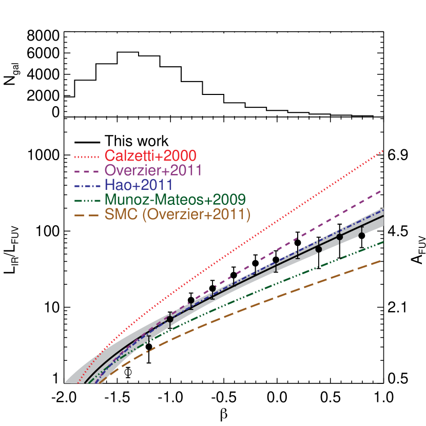
Figure 6: $L_{\rm IR}/L_{\rm FUV}$ vs. $\beta$ from stacking. Estimates with $S/N>3$ at 250, 350 and 500 $\mu$m are shown as filled circles, and others as empty circles. Lines show various $L_{\rm IR}/L_{\rm FUV}-\beta$ relations: Calzetti et al. (2000, dotted); Overzier et al. (2011, dashed); Hao et al. (2011, dot-dashed); Muñoz-Mateos et al. (2009, dot-dot-dashed); and the relation expected for the SMC extinction curve (from Overzier et al., 2011, long dashed). The solid line shows the best fit to our measurements (considering only estimates with $S/N>3$), and the grey area the range of relations implied by the 1$\sigma$ errors on the parameters. The top panel shows the number of galaxies in each bin of $\beta$.

We show on Fig. 6 the IR-to-UV luminosity ratio as a function of $\beta$. Note that the stacking results do not cover the same range in $\beta$ as in Fig. 5: the signal is small for $\beta<-1.5$.

We observe a good correlation between the UV slope and dust attenuation. We compare our results to several calibrations of the $(L_{\rm IR}/L_{\rm FUV})--\beta$ relation derived for local starburst galaxies (Calzetti et al., 2000; Overzier et al., 2011, their ‘total relation’). The difference between these two local relations comes from the fact that Overzier et al. (2011) remeasured the UV photometry for the Meurer, Heckman, & Calzetti (1999) sample, hence possibly including fewer starburst regions.

Our results fall between the local starburst and the local calibration for normal star-forming galaxies from Muñoz-Mateos et al. (2009) and the relation expected for the Small Magellanic Cloud (SMC) extinction curve. Our results are, however, consistent with the relation obtained by Hao et al. (2011) from another set of local normal star-forming galaxies, based on SINGS observations (Kennicutt et al., 2003), as well as data from Moustakas & Kennicutt (2006). Note that the spread between the calibrations from Muñoz-Mateos et al. (2009) and Hao et al. (2011) comes from differences in galaxy selections.

Following previous work we fit our measurements assuming

$$A_{\rm FUV}=2.5\log\left[\frac{1}{1.68}\left(\frac{L_{\rm{IR}}}{L_{\rm FUV}}\right)+1\right]=a+b\beta.$$ (3)

We consider only measurements with $S/N>3$ in the fit; including other measurements does not affect the results. We find $a=3.4\pm 0.1$ and $b=1.6\pm 0.1$. Our value for the slope $b=dA_{\rm FUV}/d\beta$ of this relation is lower than the values derived from commonly used local starburst attenuation laws (e.g. Meurer, Heckman, & Calzetti (1999) find $b=1.99$; Calzetti et al. (2000) find $b=2.31$), but larger than the value derived at intermediate redshifts ($1<z<2$) by Buat et al. (2011), namely $b=1.46\pm 0.21$. The implied UV slope for the dust-free case is $\beta_{0}=-2.12\pm 0.18$; this is in agreement with what is expected from stellar population models (Leitherer & Heckman, 1995), and favours a continuous star-formation mode.

5 UV and IR luminosity functions

In this section, we present our determination of the UV luminosity function of our UV sample. Using the stacking results presented above, we can also recover the total far-IR luminosity function of this sample. This procedure enables us, for instance, to discuss the dust-corrected contribution to the star-formation rate density of UV-selected galaxies.

Reddy et al. (2008) performed a similar study on a sample of LBGs at $1.9<z<3.4$. They derived the $E(B-V)$ distribution of their sample by maximising the likelihood of observing their data for a given luminosity, redshift and reddening distribution. Assuming the Meurer, Heckman, & Calzetti (1999) attenuation law, they determined the IR luminosity function of UV-selected galaxies using a Monte Carlo method and found that at $z\sim 2$ it is in agreement with the IR luminosity function of 8 $\mu$m rest-frame selected galaxies with luminosities $10^{10}\,{\rm L}_{\sun}-10^{12}\,{\rm L}_{\sun}$ range. This contrasts with the lower redshift result of Buat et al. (2009), who directly measured the IR luminosity function of UV-selected galaxies at $z\sim 1$ and noticed that it underestimates the IR luminosity function of 12 $\mu$m rest-frame selected galaxies for $L_{\rm{IR}}\ga 2\times 10^{11}\,{\rm L}_{\sun}$.

We derive luminosity functions using the $V_{\rm max}$ method (Schmidt, 1968). In practice, we derive for each galaxy of our sample the minimum ($z_{\rm min}$) and maximum ($z_{\rm max}$) redshifts where it can be included in the sample given its redshift and luminosity: $z_{\rm min}=\max(1.2,z_{\textrm{UV},\rm min})$, and $z_{\rm max}=\min(1.7,z_{\textrm{UV},\rm max})$. $z_{\textrm{UV},\rm min}$ and $z_{\textrm{UV},\rm max}$ are the minimum and maximum redshifts implied by the magnitude limits we used to build our UV-selected sample.

The maximum volume within which this galaxy can be observed is then given by:

$$V_{\rm max} = V(z_{\rm max})-V(z_{\rm min})$$ (4)

$$V(z) = \frac{A}{3}r_{\rm c}^{3}(z),$$

where $A$ is the solid angle covered by the observations, and $r_{\rm c}(z)$ is the comoving distance. We corrected for incompleteness as a function of luminosity using the simulations described Sect. 2. We define our completeness limit as the luminosity where the incompleteness is equal to 20 per cent; this corresponds to $L_{\rm FUV}=5\times 10^{9}\rm{L}_{\sun}$ and $L_{\rm IR}=5.6\times 10^{10}\rm{L}_{\sun}$. We also include the error on the completeness correction in the luminosity function errors. For each luminosity function estimate, we take into account the error on photometric redshifts by constructing 50 mock catalogues with new redshifts within the probability distribution functions derived by Ilbert et al. (2009). Note that this procedure yields an estimate of the errors added by the use of photometric redshifts, but not of the bias they introduce.

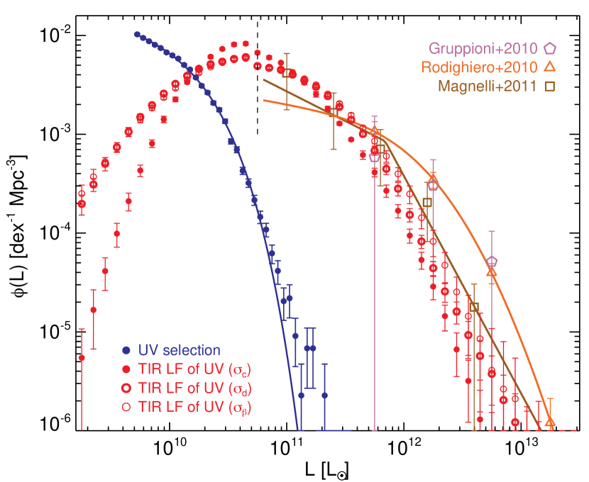
Figure 7: UV and IR luminosity functions. The blue circles represent the UV luminosity function of our sample. The red circles show the IR luminosity function of this sample derived from the stacking measurement of the IR to UV luminosity ratio: filled circles using a constant dispersion of $\log(L_{\rm{IR}}/L_{\rm FUV})$ (method ‘$\sigma_{c}$’); open thick circles the dispersion which reproduces the observed $\log(L_{\rm{IR}}/L_{\rm FUV})$ values for detected objects (‘$\sigma_{d}$’); and open thin circles the dispersion derived from the dispersion in $\beta$ slope (‘$\sigma_{\beta}$’). The dashed line shows the lower luminosity limit that we consider to adjust the IR luminosity function. Open squares show the IR luminosity function of an IR selected sample at $1.3<z<1.8$ from Magnelli et al. (2011); open triangles the IR luminosity function from Rodighiero et al. (2010) at $1.2<z<1.7$; and open hexagons the IR luminosity function from Herschel/PACS data at $1.2<z<1.7$ (Gruppioni et al., 2010).

5.1 UV luminosity function

We checked that the K-corrections are minimal and do not have an impact on the UV luminosity function. We note that the faint-end of the UV LF is quite sensitive to the method used for the photometry. The UV LF derived using the $u^{*}$-band fluxes from the catalog of Capak et al. (2007) is significantly steeper ($3\sigma$ significance level, $\alpha=-1.29\pm 0.03$) at the faint end than the measurement obtained using the photometry we use here. Capak et al. (2007) performed the source extraction in a combined $i^{+}$ and $i^{*}$ image, ran PSF matching to the image with worst seeing ($K_{s}$), and finally measured aperture photometry and aperture corrections. We attribute this difference between the LFs to an overestimation of the $u^{*}$ flux because of a combination of the PSF matching and the aperture corrections. We show our UV LF in Fig. 7 (blue circles). The error bars on the UV LF are the combination of the Poisson error, the error on the completeness correction, and the standard deviation of the estimates from the mock catalogues used to compute the LF. We fit the UV luminosity function with a Schechter form; we find $\log(\phi^{\ast}[\textrm{Mpc}^{-3}])=-2.24\pm 0.02$, $\log(L^{\ast}[{\rm L}_{\sun}])=10.13\pm 0.02$ (equivalent to $M^{*}=-19.44\pm 0.04$), and $\alpha=-1.13\pm 0.04$. We note that the luminosity function we derive is quite flat with respect to a number of previous studies devoted to estimating the UV luminosity functions at similar redshifts (Arnouts et al., 2005; Oesch et al., 2010), who report $-1.6<\alpha<-1.4$. This difference could be due to the fact that these estimates were obtained from selections using shorter restframe wavelengths than ours. However, our estimate is similar to a recent and independent derivation of the UV luminosity function by Cucciati et al. (2012), who found $\alpha=-1.09\pm 0.23$ in the same redshift range, using spectroscopic data.

5.2 Recovering the IR luminosity function

From the stacking results presented above, we recover the IR luminosity function of our UV-selected sample. To do so, we assign an IR luminosity to each of the galaxies of our sample using the following method, which is similar to that used by Reddy et al. (2008).

We assume that at a given UV luminosity, the distribution of $\log(L_{\rm{IR}}/L_{\rm FUV})$ is Gaussian. We use as the mean of this distribution the values of $L_{\rm{IR}}/L_{\rm FUV}$ derived from the stacking analysis. In the luminosity range where we do not have reliable stacking measurements ($L_{\rm FUV}>5\times 10^{10}\,{\rm L}_{\sun}$), we assume that the $L_{\rm{IR}}/L_{\rm FUV}$ ratio is constant, and equal to 6.8, the average value of the ratio over $10^{10}<L_{\rm FUV}/{\rm L}_{\sun}<5\times 10^{10}$. We also consider as mean of the $L_{\rm{IR}}/L_{\rm FUV}$ distribution the results obtained from an alternative stacking method, excluding sources detected at $10\sigma$ from the SPIRE images (see Appendix C.2).

For the standard deviation of the Gaussian distribution, we use three different methods. Firstly, (i) we assume that the dispersion of the Gaussian distribution is constant with UV luminosity and equal to 0.35. This value has been derived at low redshifts from UV-selected samples by Buat et al. (2009); we call this method ‘$\sigma_{\rm{c}}$’. Alternatively, (ii), we use as reference the values of the $L_{\rm{IR}}/L_{\rm FUV}$ ratios of the objects detected at Herschel-SPIRE wavelengths (see Sect. 2); these objects represent the upper tail of the distribution of the $L_{\rm{IR}}/L_{\rm FUV}$ ratio. We determined the mean of this distribution from stacking as a function of $L_{\rm FUV}$ (Sect. 4.1). We assume once again that the distribution of the $L_{\rm{IR}}/L_{\rm FUV}$ ratio is Gaussian. Then for each $L_{\rm FUV}$ stacking bin, we adjust the standard deviation of the Gaussian such that we reproduce the observed distribution, given the mean and the few detections in the upper tail. The resulting dispersion is a function of $L_{\rm FUV}$, and decreases from 0.5 at $L_{\rm FUV}=3\times 10^{9}{\rm L}_{\sun}$ to 0.2 at $L_{\rm FUV}=10^{11}{\rm L}_{\sun}$ (method ‘$\sigma_{\rm d}$’). Finally, (iii) we use the observed dispersion of the slope of the UV continuum, $\beta$, as a function of UV luminosity, and translate it into a dispersion in $\log(L_{\rm{IR}}/L_{\rm FUV})$, using the relation we derived in Sect. 4.2, $A_{\rm FUV}=3.4+1.6\beta$. This also yields a function of $L_{\rm FUV}$; the resulting dispersion is slightly higher than the one obtained with scenario $\sigma_{\rm d}$, decreasing from 0.6 at $L_{\rm FUV}=3\times 10^{9}{\rm L}_{\sun}$ to 0.3 at $L_{\rm FUV}=10^{11}{\rm L}_{\sun}$ (method ‘$\sigma_{\beta}$’).

For a given galaxy in our sample, we then randomly assign a value of $\log(L_{\rm{IR}}/L_{\rm FUV})$, following the relevant distribution, whose mean and standard deviation are determined by the UV luminosity of the galaxy. We can then derive the IR luminosity for each galaxy in our sample, and, using the $V_{\rm max}$ values determined according to the UV selection, compute the IR LF of the sample.

At $z=0$, all UV-selected galaxies are detected in the IR, and the distribution of $\log(L_{\rm{IR}}/L_{\rm FUV})$ is well described by a Gaussian (Buat et al., 2009). Note that the actual distribution of $\log(L_{\rm{IR}}/L_{\rm FUV})$ at $z\sim 1.5$ is not known. Assuming a Gaussian distribution enables us to compare with previous studies similar to ours (e.g. Reddy et al., 2008). However, depending on the value of the dispersion of this Gaussian, a significant number of galaxies with low $L_{\rm FUV}$ can be assigned high $L_{\rm{IR}}$.

We generate 100 realisations of this IR LF, and show on Fig. 7 the mean and errors of these iterations (red circles). We compare our result with the IR LF derived at $1.3<z<1.8$ by Magnelli et al. (2011) from a sample of galaxies selected at 24 $\mu$m and also using stacking at 70 $\mu$m (open squares), the IR LF of Rodighiero et al. (2010) (open triangles), from a sample of galaxies at $1.2<z<1.7$, also selected at 24 $\mu$m with mid-IR data, and finally the Herschel/PACS-derived IR LF from Gruppioni et al. (2010) at $1.2<z<1.7$ (open hexagons).

Our results show that correcting a UV-selected sample for dust enables us to recover the IR LF at the faint luminosities reached by the IR selections ($L_{\rm{IR}}<3\times 10^{11}\,{\rm L}_{\sun}$); our estimates are in agreement with the results of Magnelli et al. (2011) at these luminosities.

At IR luminosities brighter than $L_{\rm{IR}}=3\times 10^{11}\,{\rm L}_{\sun}$, the results depend on the assumptions about the shape of the distribution of the $L_{\rm{IR}}/L_{\rm FUV}$ ratio. A higher dispersion in this ratio yields a higher amplitude of the LF at the bright end. We note however that for the scenario with the highest dispersion, $\sigma_{\beta}$, it is not clear that the dispersion in $\beta$ is completely related to the dispersion in dust attenuation. First of all, we do not observe a stacking detection at $S/N>3$ in all Herschel-SPIRE bands for $\beta<-1.2$. Note also that the dispersion in $L_{\rm{IR}}/L_{\rm FUV}$ that we infer from the dispersion in $\beta$ is larger than the dispersion we derive from the objects directly detected by SPIRE. In any case, none of the scenarios we explore here for the dispersion of this ratio is able to reproduce accurately the bright end of the IR selected LFs. This is implied directly by the stacking results (see Fig. 4), which show that the IR luminosities of our sample galaxies are consistent with LIRGs, but not ULIRGs.

Hereafter, we consider as our best estimate the IR LF determined with the scenario $\sigma_{\rm{d}}$ described above.

5.3 Implications for Cosmic star-formation density estimation

Table 1: LF fit parameters and derived Cosmic Star-Formation rate density

IR LF from UV, DPL fit			IR LF from UV, DE fit
$\log(\phi_{\rm knee})$	$-2.70\pm 0.02$		$\log(\phi^{\ast})$	$-2.31\pm 0.04$
$\log(L_{\rm knee})$	$11.49\pm 0.02$		$\log(L^{\ast})$	$11.10\pm 0.09$
$\alpha_{2}$	$-2.10\pm 0.08$		$\sigma$	$0.41\pm 0.03$
$\alpha_{1}$	$-0.6$		$\alpha$	1.2
$\dot{\rho}_{\ast,\rm IR}\quad(10^{11}<L_{\rm{IR}}/{\rm L}_{\sun}<10^{13})$	0.08$\pm 0.01$			0.08$\pm 0.02$
$\dot{\rho}_{\ast,\rm IR}\quad(10^{7\phantom{0}}<L_{\rm{IR}}/{\rm L}_{\sun}<10^{15})$	0.16$\pm 0.01$			0.13$\pm 0.03$

DPL stands for Double Power Law, and DE for Double Exponential. $\alpha_{1}$ and $\alpha$ are kept fixed during the fitting procedure. $\phi_{\rm knee}$ and $\phi^{\ast}$ are given in Mpc^-3, $L_{\rm knee}$ and $L^{\ast}$ in ${\rm L}_{\sun}$ and $\dot{\rho}_{\ast,\rm IR}$ in $\rm{M}_{\sun}\rm{yr}^{-1}$Mpc^-3.

We study here the implications of our results for the estimation of the cosmic star-formation rate density (SFRD) from UV-selected samples.

We compute the UV luminosity density using $\dot{\rho}_{*,\rm UV}=\phi_{\ast}L_{\ast}\Gamma(\alpha+2)$, and then convert it to a star formation rate density using the relation from Kennicutt (1998):

$$SFR[\rm{M}_{\sun}\rm{yr}^{-1}]=1.4\times 10^{-28}L_{\nu}[\rm{erg}\;\rm{s}^{-1}\;\rm{Hz}^{-1}],$$ (5)

which assumes a Salpeter (1955) Initial Mass Function (IMF). We find a star-formation density $\dot{\rho}_{\ast,\rm UV}=0.022\pm 0.001\,\rm{M}_{\sun}\rm{yr}^{-1}$Mpc^-3; the error on $\dot{\rho}_{\ast,\rm UV}$ is derived from the allowed range of UV LFs within $1\sigma$ of the best fit.

IR luminosity function is commonly described by a double power law (DPL, Sanders et al., 2003):

$$\phi(L) = \phi^{\ast}\left(\frac{L}{L_{\rm knee}}\right)^{\alpha_{1}}\quad L<L_{\rm knee};$$

$$\phi(L) = \phi^{\ast}\left(\frac{L}{L_{\rm knee}}\right)^{\alpha_{2}}\quad L>L_{\rm knee}.$$ (6)

Alternatively one can use a double exponential (DE, Saunders et al., 1990):

$$\phi(L)=\phi^{*}\left(\frac{L}{L^{*}}\right)^{1-\alpha}\exp\left[-\frac{1}{\sigma^{2}}\log^{2}\left(1+\frac{L}{L^{*}}\right)\right].$$ (7)

We use both parameterisations, in order to compare with the results of Magnelli et al. (2011), who use the DPL form, and Rodighiero et al. (2010) who use the DE form. We allow to be free parameters the normalisations, $\phi_{\rm knee}$ and $\phi^{\ast}$, the characteristic luminosities, $L_{\rm knee}$ and $L^{\ast}$, and the bright-end slopes, $\alpha_{2}$ and $\sigma$. We keep the faint-end slopes fixed, using the same assumptions as Magnelli et al. (2011) ($\alpha_{1}=-0.6$) and Rodighiero et al. (2010) ($\alpha=1.2$). The best-fit parameters are given in Table 1 for our baseline IR LF.

We then integrate the IR LF within two luminosity ranges: $10^{7}<L_{\rm{IR}}/{\rm L}_{\sun}<10^{15}$, which implies an extrapolation of the measured luminosity function to faint luminosities, and $10^{11}<L_{\rm{IR}}/{\rm L}_{\sun}<10^{13}$, which is the range where observations are available. We finally convert the IR luminosity density to a SFRD using

$$SFR[\rm{M}_{\sun}\rm{yr}^{-1}]=4.5\times 10^{-44}L_{\rm{IR}}[\rm{erg}\;\rm{s}^{-1}]$$ (8)

(Kennicutt, 1998), which also assumes a Salpeter IMF. The resulting star-formation rate densities are listed in Table 1.

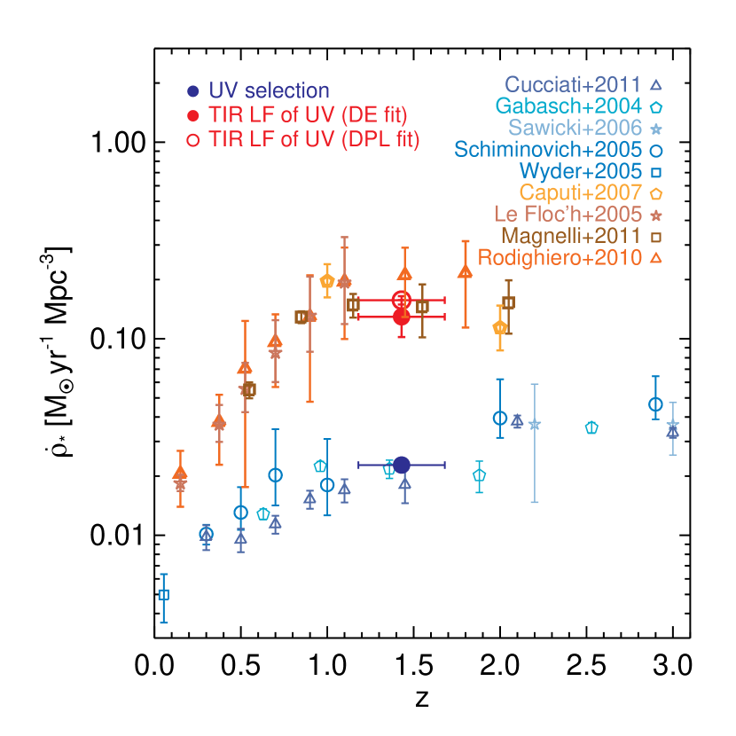
Figure 8: Cosmic star-formation rate history. Our results are represented as filled circles: UV selection (blue); and IR LF of the UV selection (red). We compare these results to the estimates based on UV-selected samples (blue-like colours): Gabasch et al. (open hexagons, 2004); Schiminovich et al. (open circles, 2005); Wyder et al. (open square, 2005); Sawicki & Thompson (open stars, 2006); and Cucciati et al. (open triangles, 2012). We also show estimates based on IR selections (red-like colours): Le Floc’h et al. (2005, open hexagons); Caputi et al. (2007, open hexagons); Rodighiero et al. (2010, open triangles); and Magnelli et al. (2011, open squares).

We consider first our most secure estimate of the SFRD, from the luminosity range where measurements are available ($10^{11}<L_{\rm{IR}}/{\rm L}_{\sun}<10^{13}$). The SFRD derived from our baseline IR LF of the UV-selected galaxies is about $89\pm 32$ per cent of the density derived from the result of Magnelli et al. (2011), and $52\pm 25$ per cent of the density derived from Rodighiero et al. (2010) from IR-selected samples. If we consider the IR LF built from the alternative stacking results, these percentages are $112\pm 41$ and $65\pm 37$ per cent.

We show our results for the cosmic star-formation rate extrapolating the luminosity function to low luminosity in Fig. 8 along with other UV-selected and IR-selected measurements (references on the figure), all integrated over the same luminosity ranges, and converted to the same IMF. The result from our UV selection is in good agreement with previous determinations of the star-formation rate density from UV-selected samples.

The cosmic SFR we derive from the IR LF of the UV selection is in broad agreement with the estimates from IR-selected samples at similar redshifts. Nevertheless, given the differences in the estimates of the SFRD from IR-selected samples, the percentage of the IR SFRD recovered by our method varies from $100\pm 33$ per cent if we consider Magnelli et al. (2011) to $61\pm 27$ per cent considering Rodighiero et al. (2010). If we consider the IR LF built from the alternative stacking method, these percentages are $131\pm 40$ and $76\pm 38$ per cent. This suggests that, after correction for dust attenuation, a UV-selected sample at $z\sim 1.5$ down to $L_{\rm FUV}=3\times 10^{9}\,\rm{L}_{\sun}$ can recover the total SFRD estimated from the IR, the remaining uncertainty being on the discrepancy between the IR-selected LFs.

Our results also imply that the dust-corrected estimate of the SFR density is roughly 6 times higher than the determination from direct UV observations.

We can compare our SFRD estimate with what would be derived using an average correction derived from $\beta$. Specifically, we derive the average attenuation factor $(\rm{SFR}_{\rm IR}+\rm{SFR}_{\rm UV})/\rm{SFR}_{\rm UV}\simeq 0.64L_{\rm IR}/L_{\rm FUV}+1$ from the distribution of $\beta$, following the same method as Bouwens et al. (2012). We use our best fit for the relation between $A_{\rm FUV}$ and $\beta$ (see Sect. 4.2). We can then determine the UV SFRD obtained from the UV LF integrated over the full data range (i.e. down to $0.2\times L_{*,\rm FUV}$), and correct it for dust attenuation with this average factor. We compare this value to the SFRD derived from the integration of the IR LF of the UV selection over the full IR luminosity range we probe. The UV SFRD corrected for dust attenuation using $\beta$ is around 25 per cent lower than the SFRD derived from the IR LF of the UV selection. This suggests that, at $z=1.5$ at least, using an average dust correction factor derived from $\beta$ can lead to a significant underestimation of the SFRD.

6 Discussion

6.1 Comparison with previous studies

There have been a number of studies exploring similar topics at lower and higher redshifts than our selection. We compare these with our results for the relation between the slope of the UV continuum and the dust attenuation, as well as the measure of the IR LF of a UV-selected sample.

6.1.1 Relation $\beta$ slope - $L_{\rm{IR}}/L_{\rm FUV}$

We find that there is a correlation between the slope of the UV continuum and the ratio $L_{\rm{IR}}/L_{\rm FUV}$. However, the relation we observe at $z=1.5$ is different from the relation that is derived from calibrations performed at low redshifts on starburst galaxies (Meurer, Heckman, & Calzetti, 1999; Calzetti et al., 2000). This starburst relation is commonly used over a wide redshift range to correct UV luminosities for dust attenuation when far-IR measurements are not available (e.g. Adelberger & Steidel, 2000; Schiminovich et al., 2005; Bouwens et al., 2009).

It is claimed that the Meurer, Heckman, & Calzetti (1999) and Calzetti et al. (2000) relations are valid at various redshifts: Reddy et al. (2006a) show that typical $z\sim 2$ UV-selected galaxies detected at 24 $\mu$m do follow the Meurer et al. relation. Magdis et al. (2010a) and Magdis et al. (2010b) also find that the UV star-formation rates of Lyman Break Galaxies at $z\sim 3$ corrected for attenuation with the Meurer, Heckman, & Calzetti (1999) relation are in agreement with far-IR and radio estimates. Reddy et al. (2006a) find, however, that the dust attenuation is overestimated for galaxies with younger stellar populations; they also show that galaxies with lower SFRs tend to lie under the Meurer, Heckman, & Calzetti (1999) relation. Burgarella et al. (2007) notice that UV star-formation rates corrected for dust attenuation with the Meurer et al. relation are in agreement with IR-derived ones, but that the dispersion is large. In a study similar to ours, Reddy et al. (2012) perform stacking of $z\sim 2$ Lyman Break Galaxies at 24, 100 and 160 $\mu$m, as well as 1.4 GHz. They find that the average $L_{\rm{IR}}/L_{\rm FUV}$ ratio of these $L_{\ast}$ Lyman Break Galaxies is consistent with the local starburst relation.

While our result hence might seem at odds with previous work, a number of studies have shown that attempting to correct for dust attenuation using the slope of the UV continuum is quite complex, and requires some caution.

At low redshift, Bell (2002), Boissier et al. (2007), Muñoz-Mateos et al. (2009), and Seibert et al. (2005) showed that the $\beta$ slope and the dust attenuation of normal star-forming galaxies do not follow the same relationship as for local starbursts; in this case the Meurer, Heckman, & Calzetti (1999) relation overpredicts the dust attenuation, which is in agreement with our results. The validity of the starburst relation depends also on the sample selection: for local galaxies dust attenuation might be overestimated for a UV-selected sample, while underestimated for IR-selected samples (Buat et al., 2005; Seibert et al., 2005). On the other hand, at higher redshifts ($0.66<z<2.6$), Murphy et al. (2011) observed that the Meurer, Heckman, & Calzetti (1999) relation overpredicts the dust attenuation for 24 $\mu$m selected galaxies. Note also that Buat et al. (2010) found that at $z<0.3$, galaxies selected at 250 $\mu$m have dust attenuations between the local starbursts and the normal star forming relation from Boissier et al. (2007). The mean relation that we derive here is actually in excellent agreement with their results. We note also that our sample is dominated by galaxies of IR luminosities similar to LIRGs. At $z\sim 1.5$, these galaxies belong mostly to the ‘main sequence’ of star forming galaxies and are not in the starburst mode (Sargent et al., 2012), which can partly explain why the relation between $\beta$ and the dust attenuation we obtain is similar to normal star forming galaxies at low redshifts.

The variety of results presented above is linked to the fact that the UV and IR emissions can come from different regions in the galaxies, and also that attempting to use the slope of the UV continuum to correct for dust attenuation requires assumptions about the underlying extinction law and star-formation history. Using the Meurer, Heckman, & Calzetti (1999) or the Calzetti et al. (2000) relations is consistent with using quite shallow extinction laws, such as the Calzetti, Kinney, & Storchi-Bergmann (1994) or Calzetti (1997) ones, which is equivalent to adopting a clumpy foreground distribution of dust. Our results (in terms of the slope of the $A_{\rm FUV}-\beta$ relation) suggest a steeper extinction law, which is expected for dust geometries similar to a foreground screen. Note however that using the SMC extinction law yields a relation lower than our results, and hence is too steep. On the other hand, the value of the dust-free slope we derive suggests that the star formation mode is more continuous rather than starburst.

In summary, our result for the $\beta$ slope - $L_{\rm{IR}}/L_{\rm FUV}$ relation at $=1.5$ is similar to those obtained from local normal star forming galaxies. This suggests that our sample galaxies have a steeper extinction law than those from Calzetti, Kinney, & Storchi-Bergmann (1994) and Calzetti (1997), but less steep than the SMC one. This also shows that using a $\beta$ slope - $L_{\rm{IR}}/L_{\rm FUV}$ relation calibrated on local starburts galaxies can induce an overestimation of the $L_{\rm{IR}}/L_{\rm FUV}$ from the $\beta$ slope by around a factor of 2.

6.1.2 IR LF of UV-selected sample

We find that the IR LF of a UV-selected sample at $z\sim 1.5$ down to $L_{\rm FUV}=3\times 10^{9}\,\rm{L}_{\odot}$ recovers the faint-end of the IR LF of far-IR selected samples, but might underestimate the bright-end, if we consider the latest Herschel results, and our most conservative stacking measures.

These results are in agreement with those of Buat et al. (2009) ($z\sim 1$) who found that the bolometric ($L=L_{\rm UV}+L_{\rm{IR}}$) LF of a UV selection directly measured from UV and IR data underestimates the IR LF from IR selected sample for $L>2\times 10^{11}\,{\rm L}_{\sun}$. At higher redshifts, Reddy et al. (2008) performed a similar study, and found, on the contrary, that the reconstructed IR LF of UV-selected samples at $z=2$ and $z=3$ is similar to the IR LF of IR-selected samples. Note that we use a method which is quite similar to that of Reddy et al. (2008) to build our IR LF. In detail, Reddy et al. (2008) reconstruct two IR LFs: one from the distribution of $E(B-V)$ derived from a maximum likelihood analysis; and the other one using previously observed $L_{\rm{IR}}/L_{\rm FUV}$ ratios and dispersion. These two LFs are consistent with each other. We note that their method of using the distribution of $E(B-V)$ assumes the Calzetti et al. (2000) relation, which does not seem to apply to our sample (Sect. 6.1.1). In other words, since using the Calzetti et al. (2000) relation on our sample would yield larger dust-corrected luminosities, this can explain part of the discrepancy.

The other method used by Reddy et al. (2008) is based on previous determinations of the IR-to-UV ratio and its dispersion ($L_{\rm{IR}}/L_{\rm FUV}=4.7$, $\sigma(\log(L_{\rm{IR}}/L_{\rm FUV}))=0.53$, Reddy et al., 2006a). This average IR-to-UV ratio is lower than the values we derive here, while the dispersion is higher. In order to test the impact of our assumptions on the recovery of the bright-end of the IR LF, we used as an extreme case the values of $L_{\rm{IR}}/L_{\rm FUV}$ we obtained here, and the dispersion used by Reddy et al. (2008) to construct the IR LF from the UV selection. The results we thus obtain (see filled squares on fig. 9) are in agreement with the IR LF of Magnelli et al. (2011, based on Spitzer data), but then slightly underestimate the measurements of Rodighiero et al. (2010, also based on Spitzer data) and Gruppioni et al. (2010, based on Herschel PACS data). While this result is in better agreement with the LFs obtained from IR-selected samples, we believe that a constant dispersion of the $(L_{\rm{IR}}/L_{\rm FUV})$ with $L_{\rm FUV}$ is unlikely. Based on our sample, we observe that the dispersion around $(L_{\rm{IR}}/L_{\rm FUV})$ decreases with $L_{\rm FUV}$, either from the dispersion in $\beta$ or from the dispersion which is required to reproduce the $(L_{\rm{IR}}/L_{\rm FUV})$ values of the few UV-selected galaxies detected at the SPIRE wavelengths. Note also that using this value of the dispersion would imply, for instance, around four times as many ULIRGs as we detect with SPIRE. We also attempted to adjust the dispersion required to match the IR LF of Rodighiero et al. (2010), assuming an exponentialy decreasing function of $L_{\rm FUV}$, as we observe in the data. The best fit in this case implies twice as many ULIRGs as we detect.

6.1.3 Contribution to the CIB of UV-selected sources

Our results for the IR LF of our UV-selected sample imply that a UV-selection misses a significant part of the IR galaxy population, at least within the UV luminosity range we are able to probe. To investigate this further, we measured the contribution to the Cosmic Infrared Background (CIB) at the SPIRE wavelengths from the UV-selected galaxies in our sample, and compared it to the values measured by Béthermin et al. (2012), who derived the contribution to the CIB from 24 $\mu$m-selected sources with $S_{24}>80\,\mu$Jy. We measured by stacking the average flux density for galaxies in two redshift bins ($1.2<z<1.4$ and $1.4<z<1.6$), and converted it to a surface brightness. We find that the contribution to the CIB from our UV-selected galaxies is lower than that from 24$\mu$m-selected sources. The contribution to the CIB from our UV-selected galaxies is around 50 per cent of that from 24 $\mu$m-selected sources for $1.2<z<1.4$ and around 30 per cent for $1.4<z<1.6$. This result clearly shows that a UV selection is missing a part of the galaxy population probed by IR selections, and that the amount of energy which is emitted by this missing population is a significant fraction of the CIB.

6.2 Recovering the bright-end of the IR LF

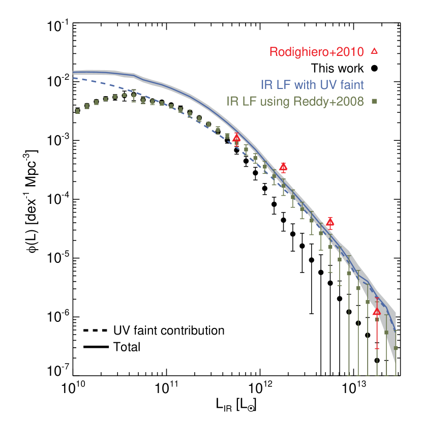
Figure 9: Recovering the bright-end of the IR LF. Filled circles show the IR LF of our UV selection, based on available data. The solid line show the total IR LF of the UV selection including the contribution of fainter galaxies ($10^{8}<L_{\rm FUV}/{\rm L}_{\sun}<10^{9.5}$) adjusted to match the result of Rodighiero et al. (2010). The dashed line show the contribution to the IR LF of the faint UV galaxies. The shaded grey area shows the range of LFs implied by the $1\sigma$ errors on the parameters. We assume here that the dispersion of the ratio $\log(L_{\rm{IR}}/L_{\rm FUV})$ is a constant for galaxies with $10^{8}<L_{\rm FUV}/{\rm L}_{\sun}<10^{9.5}$. The filled squares show the IR LF of the UV selection (no extrapolation to luminosities fainter than our limit) we obtain if we use our stacking measurements for $\log(L_{\rm{IR}}/L_{\rm FUV})$ and the dispersion on this ratio used by Reddy et al. (2008).

Using our most conservative stacking measurements, our results show that the IR LF we build for our UV-selected sample does not recover the bright-end of the measured IR LF from IR-selected samples, if we consider the latest Herschel estimates. This would imply that a part of the IR galaxy population is missed by UV selection, at least in the redshift and luminosity ranges we consider here. We investigate the possibility that this missing population is actually fainter in UV luminosity than the limit reached by our observations. Note that according to our results shown in Fig. 4, the galaxies in our UV-selected sample are mostly similar to LIRGs, hence we have to populate the ULIRGs regime of the luminosity function, which requires a large dispersion of the $L_{\rm{IR}}/L_{\rm FUV}$ ratio.

To do so, we extrapolate the UV luminosity function down to $L_{\rm FUV}=10^{8}\,{\rm L}_{\sun}$, using the best fit we obtain (see Sect. 5.1). This corresponds to a magnitude limit $u^{*}=29.75$ mag, 3.75 magnitudes deeper than the data we are using. In practice we create a mock catalogue which has the proper luminosity function. Then we compute the IR LF of this mock catalogue using the same method described in Sect. 5.2. In this case, however, we do not have measurements for the mean IR-to-UV ratio or the dispersion of this ratio. We rather adjust these two quantities such that the sum of the IR LF of the mock catalogue and the IR LF of the UV selection from our baseline stacking method is consistent with the IR LF of Rodighiero et al. (2010).

As we are limited by the relatively poor observational constraints on the IR LF, we make the following simplistic assumptions: we consider that the ratio $L_{\rm{IR}}/L_{\rm FUV}$ and the dispersion around this ratio are constant over the range $10^{8}<L_{\rm FUV}/{\rm L}_{\sun}<3\times 10^{9}$; we then use two free parameters, $\langle L_{\rm{IR}}/L_{\rm FUV}\rangle$ and $\sigma\left(\log(L_{\rm{IR}}/L_{\rm FUV})\right)$, to adjust the contribution of UV faint galaxies to the bright-end of the IR LF.

The results of the fit are shown Fig. 9. The contribution to the IR LF of the faint UV galaxies is shown as the dashed line, and the total IR LF as the solid line. These results show that it is possible to obtain parameters that fit the IR LF measured from IR-selected samples. We find $\langle L_{\rm{IR}}/L_{\rm FUV}\rangle=8.7^{+3.1}_{-2.7}$ and $\sigma(\log(L_{\rm{IR}}/L_{\rm FUV}))=0.73^{+0.04}_{-0.06}$. The average IR to UV ratio required to match the bright-end of the IR LF is consistent with the value we measure in our two faintest bins at $L_{\rm FUV}=(3-4)\times 10^{9}\,{\rm L}_{\sun}$ ($L_{\rm{IR}}/L_{\rm FUV}=14.5\pm 6,11.5\pm 5$), while the requested dispersion of the ratio is larger than what we observe: at $L_{\rm FUV}=3\times 10^{9}\,{\rm L}_{\sun}$ the dispersion required to match the detected objects is $\sigma(\log(L_{\rm{IR}}/L_{\rm FUV}))=0.5$.

From this fit we can estimate the fraction of galaxies that is missed by a UV selection, compared to an IR selection. We integrate the IR LF of the faint UV galaxies in the range $6.5\times 10^{10}<L_{\rm{IR}}/{\rm L}_{\sun}<10^{13}$, where data are available, and compare this density to the one derived by integrating the total IR LF in the same range. We find that in terms of number density, 56 per cent of galaxies are missed.

The relatively poor constraints on the IR LF do not enable us to draw firm conclusions on the scenarios of dust attenuation for faint UV galaxies. Note that the shape of the IR LF is quite sensitive to the assumptions on the dispersion $\sigma(\log(L_{\rm{IR}}/L_{\rm FUV}))$. Hence we expect to set better constraints on these scenarios with updated Herschel LFs.

7 Summary and Conclusions

We used Herschel-SPIRE (Griffin et al., 2010; Swinyard et al., 2010) imaging from the HerMES (Oliver et al., 2012) programme to study the IR properties of a sample of UV-selected galaxies at $z\sim 1.5$ in the COSMOS field. We built our sample from galaxies detected in CFHT $u^{*}$ band (Capak et al., 2007) down to $u^{*}=26$ mag, with photometric redshifts (Ilbert et al., 2009) $1.2<z_{\rm phot}<1.7$. Only a few per cent of these galaxies are detected at the Herschel-SPIRE wavelengths, so we use stacking in order to derive the average IR luminosities of the galaxies as a function of $L_{\rm FUV}$ and the slope of the UV continuum $\beta$. We detail the techniques we used to correct the stacking measurements from stacking bias and clustering of the UV-selected galaxies, based on extensive simulations. We use these stacking measurements to derive the IR LF of the UV-selected sample, in order to infer the cosmic star formation rate density probed by a UV selection at $z=1.5$. Our conclusions are as follows:

1. UV-selected galaxies at $z=1.5$ and $4\times 10^{9}<L_{\rm FUV}/\rm{L}_{\sun}<5\times 10^{10}$ have average total IR luminosities similar to LIRGs, but not to ULIRGs.

2. The average $L_{\rm{IR}}/L_{\rm FUV}$ ratio is roughly constant, with $L_{\rm FUV}$ ($4\times 10^{9}<L_{\rm FUV}/{\rm L}_{\sun}<5\times 10^{10}$) and is equal to $6.9\pm 1.$

3. The average $L_{\rm{IR}}/L_{\rm FUV}$ ratio is correlated with the slope of the UV continuum, $\beta$. This relation is below the relation derived from local starburst galaxies, but is in agreement with previous results obtained from local normal star-forming galaxies. Our best fit to this relation is $A_{\rm FUV}=3.4\pm 0.1+(1.6\pm 0.1)\beta$.

4. We built the IR LF of the UV sample using our stacking measurements of the average $L_{\rm IR}/L_{\rm FUV}$ ratio, and assuming that the distribution of $\log(L_{\rm IR}/L_{\rm FUV})$ is Gaussian. We used three different scenarios for the value of the dispersion $\sigma(\log(L_{\rm IR}/L_{\rm FUV}))$, which all yield the same result that the IR LF of the UV sample is in reasonable agreement at the faint-end ($L_{\rm{IR}}\sim 10^{11}\,{\rm L}_{\sun}$) with the IR LF from IR-selected samples at the same epoch, but might underestimate it at the bright-end ($L_{\rm{IR}}\ga 5\times 10^{11}\,{\rm L}_{\sun}$).

5. At $z\sim 1.5$ a UV rest-frame selection without dust attenuation correction probes roughly 10 per cent of the total (UV+IR) star-formation rate density. The cosmic star-formation rate density derived from the IR LF of the UV sample corresponds to 61–76 per cent or 100–133 per cent of the star-formation rate density derived from IR-selected samples, depending on the IR LF taken as reference (Rodighiero et al. 2010 or Magnelli et al. 2011).

6. Assuming our most conservative measures and the latest Herschel estimates, the fraction of galaxies which are missed by a UV selection compared to an IR selection at $z\sim 1.5$ is around 50 per cent, in terms of number density; this number is sensitive to the assumptions on the dispersion $\sigma(\log(L_{\rm IR}/L_{\rm FUV}))$.

Appendix A Stacking results

Table 2: Stacking results as a function of $L_{\rm FUV}$

$\log(L_{\rm FUV}[L_{\odot}])$ range	$\langle\log(L_{\rm FUV}[L_{\odot}])\rangle$	$\langle z\rangle$	$N_{gal}$	$S_{250}$ [mJy]	$S_{350}$ [mJy]	$S_{500}$ [mJy]	$\log(L_{\rm IR}[L_{\odot}])$
9.44 – 9.54	9.51	1.26	872	0.71 $\pm$ 0.24	0.84 $\pm$ 0.21	0.81 $\pm$ 0.27	10.67 $\pm$ 0.20
9.54 – 9.64	9.60	1.34	3075	0.66 $\pm$ 0.12	0.72 $\pm$ 0.16	0.52 $\pm$ 0.15	10.66 $\pm$ 0.18
9.64 – 9.74	9.70	1.43	5760	0.46 $\pm$ 0.08	0.58 $\pm$ 0.10	0.44 $\pm$ 0.10	10.54 $\pm$ 0.11
9.74 – 9.84	9.79	1.46	6018	0.43 $\pm$ 0.10	0.53 $\pm$ 0.10	0.36 $\pm$ 0.09	10.54 $\pm$ 0.17
9.84 – 9.94	9.89	1.44	5383	0.63 $\pm$ 0.09	0.69 $\pm$ 0.11	0.54 $\pm$ 0.10	10.67 $\pm$ 0.12
9.94 – 10.04	9.99	1.44	4631	0.65 $\pm$ 0.10	0.66 $\pm$ 0.12	0.48 $\pm$ 0.10	10.71 $\pm$ 0.18
10.04 – 10.14	10.09	1.44	3883	0.88 $\pm$ 0.11	0.89 $\pm$ 0.13	0.59 $\pm$ 0.11	10.86 $\pm$ 0.17
10.14 – 10.24	10.19	1.43	3052	1.35 $\pm$ 0.13	1.40 $\pm$ 0.16	1.02 $\pm$ 0.13	10.99 $\pm$ 0.10
10.24 – 10.34	10.29	1.43	2177	1.54 $\pm$ 0.17	1.42 $\pm$ 0.16	0.90 $\pm$ 0.14	11.14 $\pm$ 0.18
10.34 – 10.44	10.39	1.43	1503	1.87 $\pm$ 0.21	1.79 $\pm$ 0.20	1.10 $\pm$ 0.19	11.22 $\pm$ 0.19
10.44 – 10.54	10.49	1.44	873	2.43 $\pm$ 0.25	2.38 $\pm$ 0.29	1.60 $\pm$ 0.26	11.29 $\pm$ 0.15
10.54 – 10.64	10.59	1.44	463	3.45 $\pm$ 0.40	3.32 $\pm$ 0.43	2.10 $\pm$ 0.34	11.47 $\pm$ 0.19
10.64 – 10.74	10.69	1.44	211	3.66 $\pm$ 0.61	3.39 $\pm$ 0.61	1.99 $\pm$ 0.54	11.56 $\pm$ 0.24
10.74 – 10.84	10.78	1.43	111	3.56 $\pm$ 0.77	3.09 $\pm$ 0.85	2.42 $\pm$ 0.85	11.50 $\pm$ 0.31
10.84 – 10.94	10.89	1.45	35	3.85 $\pm$ 1.62	2.46 $\pm$ 1.92	0.00 $\pm$ 0.75	11.18 $\pm$ 0.96
10.94 – 11.04	10.99	1.43	16	9.50 $\pm$ 1.58	7.50 $\pm$ 1.97	4.69 $\pm$ 1.92	11.99 $\pm$ 0.36
11.04 – 11.14	11.07	1.52	5	3.97 $\pm$ 2.36	3.89 $\pm$ 3.51	4.50 $\pm$ 4.69	11.59 $\pm$ 0.58
11.14 – 11.24	11.19	1.44	5	22.96 $\pm$ 8.25	22.23 $\pm$ 7.21	17.63 $\pm$ 5.04	12.28 $\pm$ 0.25

Table 3: Stacking results as a function of $\beta$

$\beta$ range	$\langle\beta\rangle$	$\langle\log(L_{\rm FUV}[L_{\odot}])\rangle$	$\langle z\rangle$	$N_{gal}$	$S_{250}$ [mJy]	$S_{350}$ [mJy]	$S_{500}$ [mJy]	$\log(L_{\rm IR}[L_{\odot}])$
-2.50 – -2.30	-2.39	9.92	1.46	418	0.00 $\pm$ 0.03	0.08 $\pm$ 0.17	0.17 $\pm$ 0.23	8.46 $\pm$ 0.72
-2.30 – -2.10	-2.19	9.98	1.46	921	0.00 $\pm$ 0.00	0.00 $\pm$ 0.00	0.00 $\pm$ 0.00	0.00 $\pm$ 0.00
-2.10 – -1.90	-1.99	9.98	1.45	1877	0.00 $\pm$ 0.00	0.00 $\pm$ 0.00	0.00 $\pm$ 0.00	0.00 $\pm$ 0.00
-1.90 – -1.70	-1.79	10.04	1.45	3448	0.00 $\pm$ 0.00	0.00 $\pm$ 0.00	0.00 $\pm$ 0.00	0.00 $\pm$ 0.00
-1.70 – -1.50	-1.60	10.05	1.45	4984	0.00 $\pm$ 0.00	0.00 $\pm$ 0.00	0.03 $\pm$ 0.04	6.25 $\pm$ 0.66
-1.50 – -1.30	-1.40	10.07	1.44	6081	0.19 $\pm$ 0.02	0.38 $\pm$ 0.09	0.28 $\pm$ 0.10	10.22 $\pm$ 0.07
-1.30 – -1.10	-1.20	10.07	1.43	5725	0.44 $\pm$ 0.09	0.52 $\pm$ 0.11	0.38 $\pm$ 0.11	10.55 $\pm$ 0.17
-1.10 – -0.90	-1.00	10.05	1.42	4705	1.11 $\pm$ 0.10	1.09 $\pm$ 0.11	0.84 $\pm$ 0.10	10.89 $\pm$ 0.10
-0.90 – -0.70	-0.81	10.02	1.41	3321	1.76 $\pm$ 0.13	1.79 $\pm$ 0.12	1.18 $\pm$ 0.10	11.11 $\pm$ 0.11
-0.70 – -0.50	-0.61	9.99	1.41	2109	2.31 $\pm$ 0.17	2.22 $\pm$ 0.17	1.44 $\pm$ 0.15	11.24 $\pm$ 0.12
-0.50 – -0.30	-0.41	9.99	1.40	1325	3.40 $\pm$ 0.22	3.08 $\pm$ 0.24	2.09 $\pm$ 0.20	11.41 $\pm$ 0.12
-0.30 – -0.10	-0.20	9.96	1.39	899	4.59 $\pm$ 0.30	4.10 $\pm$ 0.32	2.72 $\pm$ 0.27	11.54 $\pm$ 0.13
-0.10 – 0.10	-0.01	9.94	1.38	604	4.88 $\pm$ 0.38	4.48 $\pm$ 0.40	2.88 $\pm$ 0.33	11.56 $\pm$ 0.14
0.10 – 0.30	0.19	9.87	1.37	411	6.38 $\pm$ 0.49	5.57 $\pm$ 0.45	3.42 $\pm$ 0.43	11.72 $\pm$ 0.16
0.30 – 0.50	0.39	9.87	1.36	266	6.18 $\pm$ 0.79	5.71 $\pm$ 0.71	3.74 $\pm$ 0.54	11.63 $\pm$ 0.19
0.50 – 0.70	0.59	9.83	1.36	164	6.26 $\pm$ 0.59	5.48 $\pm$ 0.65	3.17 $\pm$ 0.59	11.75 $\pm$ 0.20
0.70 – 0.90	0.79	9.77	1.34	107	8.44 $\pm$ 1.05	8.68 $\pm$ 0.99	5.69 $\pm$ 0.72	11.71 $\pm$ 0.13

Appendix B Stacking postage stamp images

We display here only the stacking results with signal-to-noise ratios larger than 3 at 250, 350 and 500 $\mu$m. This signal-to-noise ratio is the ratio of the flux density over the error on the flux density after the corrections described in Sect. 3 have been applied. We show here the raw stacking images, before applying any correction. All stack images are 240 arcsec accross. The gray-scale shows the signal, using a asinh stretch (Lupton et al., 2004). Each panel uses a different scale, driven by the maximum flux. We also show for reference the radial profile along with the fit by the proper PSF in each band.

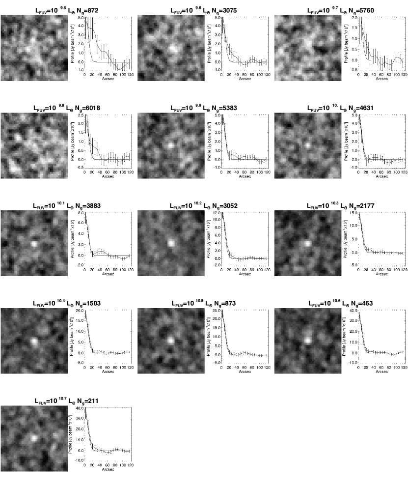
Figure 10: Stacking postage stamp images at 250 $\mu$m in bins of $L_{\rm FUV}$. $N_{g}$ is the number of UV-selected galaxies in each bin.

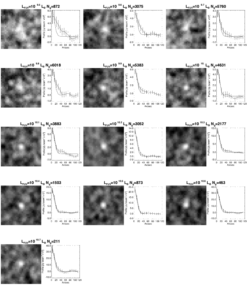
Figure 11: Stacking postage stamp images at 350 $\mu$m in bins of of $L_{\rm FUV}$.

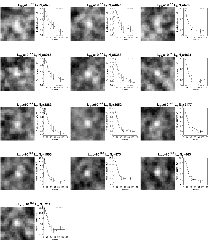
Figure 12: Stacking postage stamp images at 500  $\mu$m in bins of of $L_{\rm FUV}$.

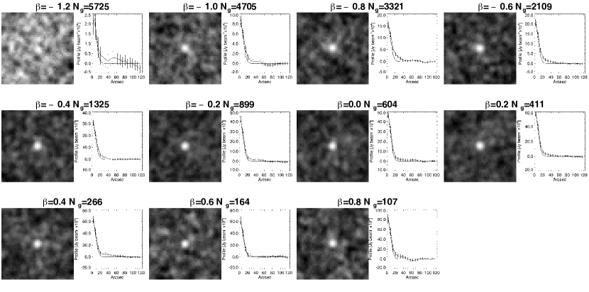
Figure 13: Stacking postage stamp images at 250 $\,\mu$m in bins of $\beta$, the UV slope.

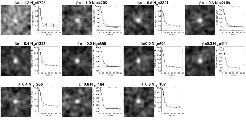
Figure 14: Stacking postage stamp images at 350 $\mu$m in bins of $\beta$, the UV slope.

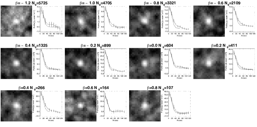
Figure 15: Stacking postage stamp images at 500 $\mu$m in bins of $\beta$, the UV slope.

Appendix C Comparison with other stacking methods

C.1 Comparison of mean stacking versus median stacking

In Fig. 16 we show a comparison of the results obtained with our method with those obtained using median stacking. This figure is similar to Fig. 4. We show in black circles the results obtained with our method, and in orange squares the results obtained with median stacking. For the latter, we perform median stacking, correcting only for clustering as described in Sect. 3.2, but not correcting for stacking bias (Sect. 3.1). The agreement between the results from mean and median stacking is excellent.

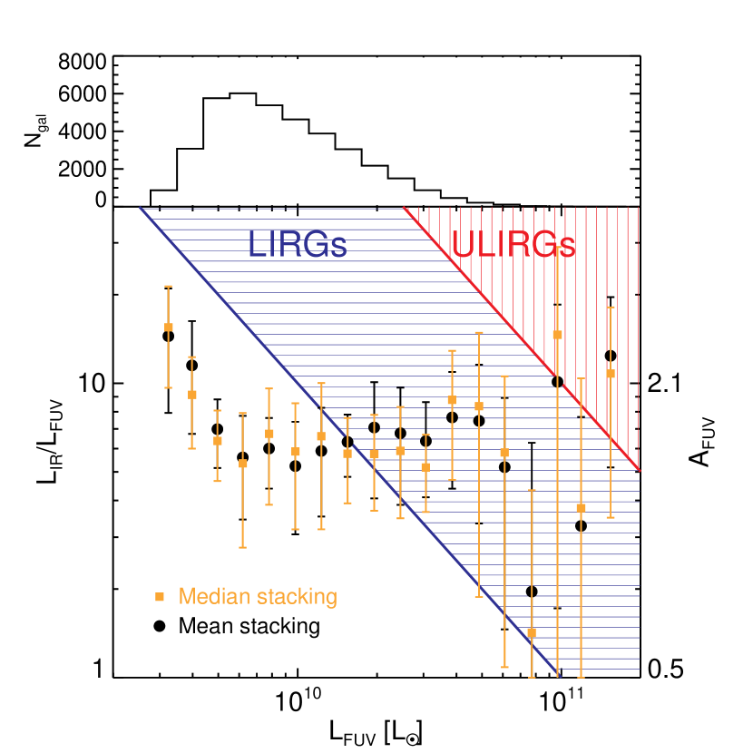
Figure 16: IR-to-UV luminosity ratio as a function of UV luminosity. Circles show estimates using the method we describe in this paper. Squares show estimates using median stacking, correcting for clustering only. The horizontally hatched region represents the locus of LIRGs, while the vertically hatched region is for ULIRGs. The right axis shows the equivalent attenuation in the FUV band (in magnitudes), using eq. 2. The top panel shows the histogram of galaxies as a function of $L_{\rm FUV}$.

C.2 Comparison of stacking with and without subtraction of detected sources

We compare in Fig. 17 the results of our method with another approach where we subtract detected sources from the images prior stacking. In practice we perform stacking after subtracting from the images the sources detected either at 3$\sigma$ or 10$\sigma$ in each SPIRE band. We use mean stacking, correcting only for clustering as described in Sect. 3.2, but not correcting for stacking bias (Sect. 3.1). To obtain the final estimate, we add to the stacked flux measure the flux of the UV-selected sources detected with SPIRE which were subtracted. The resulting fluxes are on average 20 per cent higher than those obtained with our main method, even if they are in agreement at the $1\sigma$ level, and do not depend significantly on the threshold used for subtracting sources. We show in Fig. 18 the IR LF built using the method $\sigma_{d}$ (see Sect. 5.2) and these stacking measurements, and compare it to the results obtained with our baseline stacking results. This IR LF has a slightly larger amplitude at the bright end than the one obtained from our baseline results, and is hence in better agreement with the LF of Magnelli et al. (2011).

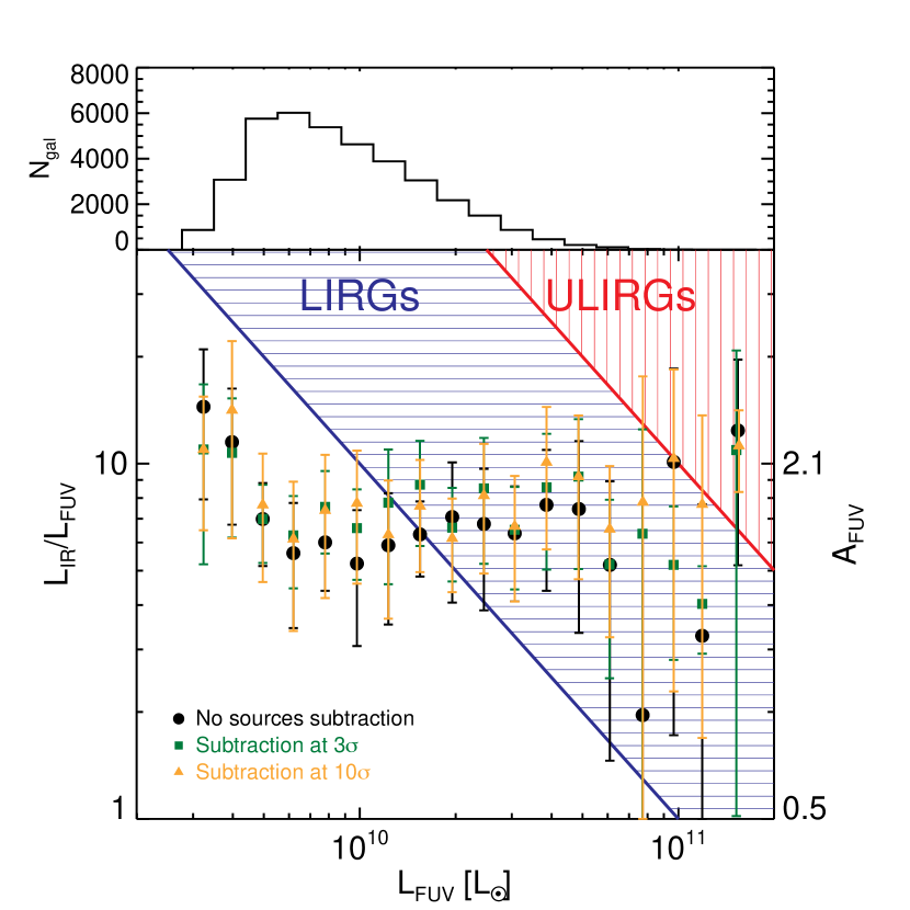
Figure 17: IR-to-UV luminosity ratio as a function of UV luminosity. Squares (respectively triangles) show the mean stacking results obtained while subtracting from the images the sources detected at 3$\sigma$ (respectively 10$\sigma$) in each band, correcting from clustering only. Circles show the results obtained with the method described in this paper. The horizontally hatched region represents the locus of LIRGs, while the vertically hatched region is for ULIRGs. The right axis shows the equivalent attenuation in the FUV band (in magnitudes), using eq. 2. The top panel shows the histogram of galaxies as a function of $L_{\rm FUV}$.

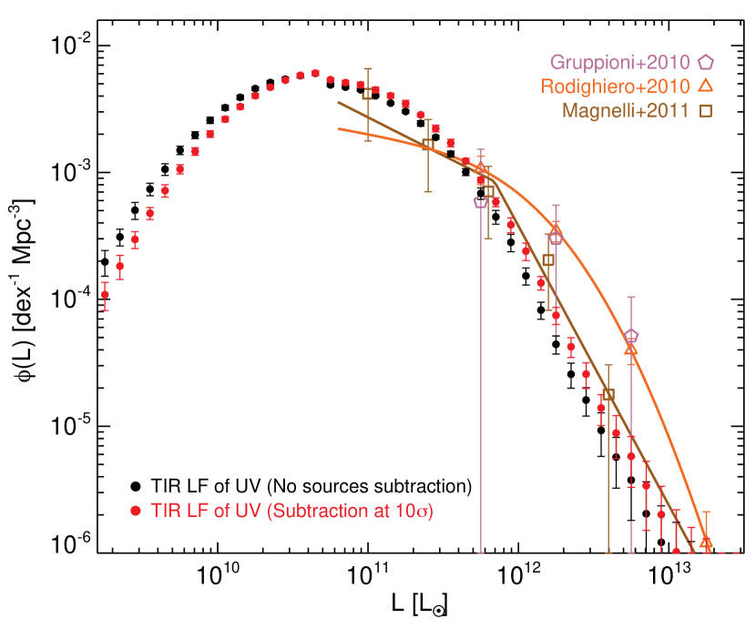
Figure 18: IR luminosity functions. The filled circles show the IR luminosity function of our sample derived from the stacking measurement of the IR to UV luminosity ratio: the black circles using the dispersion which reproduces the observed $\log(L_{\rm{IR}}/L_{\rm FUV})$ values for detected objects (‘$\sigma_{d}$’) and our baseline stacking measurements; the red circles using the same scenario for the dispersion $\sigma_{d}$, but using the stacking measurements obtained while subtracting from the images the sources detected at 10$\sigma$ in each band. Open squares show the IR luminosity function of an IR selected sample at $1.3<z<1.8$ from Magnelli et al. (2011); open triangles the IR luminosity function from Rodighiero et al. (2010) at $1.2<z<1.7$; and open hexagons the IR luminosity function from Herschel/PACS data at $1.2<z<1.7$ (Gruppioni et al., 2010).

References

- Adelberger & Steidel (2000) Adelberger K. L., Steidel C. C., 2000, ApJ, 544, 218
- Arnouts et al. (2005) Arnouts S., et al., 2005, ApJ, 619, L43
- Bavouzet et al. (2008a) Bavouzet N., Dole H., Le Floc’h E., Caputi K. I., Lagache G., Kochanek C. S., 2008, A&A, 479, 83
- Bavouzet (2008b) Bavouzet N., 2008b, PhD thesis, Université Paris-Sud XI, http://tel.archives-ouvertes.fr/docs/00/36/39/75/PDF/these_nb.pdf
- Bell (2002) Bell E. F., 2002, ApJ, 577, 150
- Bertin & Arnouts (1996) Bertin E., Arnouts S., 1996, A&AS, 117, 393
- Béthermin et al. (2010a) Béthermin M., Dole H., Beelen A., Aussel H., 2010a, A&A, 512, A78
- Béthermin et al. (2010b) Béthermin M., Dole H., Cousin M., Bavouzet N., 2010b, A&A, 516, A43
- Béthermin et al. (2012) Béthermin M., et al., 2012, A&A, 542, A58
- Boissier & Prantzos (2001) Boissier S., Prantzos N., 2001, MNRAS, 325, 321
- Boissier et al. (2007) Boissier S., et al., 2007, ApJS, 173, 524
- Bothwell et al. (2011) Bothwell M. S., et al., 2011, MNRAS, 415, 1815
- Bouwens et al. (2009) Bouwens R. J., et al., 2009, ApJ, 705, 936
- Bouwens et al. (2010) Bouwens R. J., et al., 2010, ApJ, 708, L69
- Bouwens et al. (2012) Bouwens R. J., et al., 2012, ApJ, 754, 83
- Buat et al. (2005) Buat V., et al., 2005, ApJ, 619, L51
- Buat et al. (2009) Buat V., Takeuchi T. T., Burgarella D., Giovannoli E., Murata K. L., 2009, A&A, 507, 693
- Buat et al. (2010) Buat V., et al., 2010, MNRAS, 409, L1
- Buat et al. (2011) Buat V., et al., 2011, A&A, 533, A93
- Burgarella et al. (2007) Burgarella D., Le Floc’h E., Takeuchi T. T., Huang J. S., Buat V., Rieke G. H., Tyler K. D., 2007, MNRAS, 380, 986
- Calzetti, Kinney, & Storchi-Bergmann (1994) Calzetti D., Kinney A. L., Storchi-Bergmann T., 1994, ApJ, 429, 58
- Calzetti (1997) Calzetti D., 1997, AJ, 113, 162
- Calzetti et al. (2000) Calzetti D., Armus L., Bohlin R. C., Kinney A. L., Koornneef J., Storchi-Bergmann T., 2000, ApJ, 533, 682
- Calzetti (2001) Calzetti D., 2001, PASP, 113, 1449
- Capak et al. (2007) Capak P., et al., 2007, ApJS, 172, 99
- Caputi et al. (2007) Caputi K. I., et al., 2007, ApJ, 660, 97
- Cortese et al. (2006) Cortese L., et al., 2006, ApJ, 637, 242
- Cucciati et al. (2012) Cucciati O., et al., 2012, A&A, 539, A31
- Dale & Helou (2002) Dale D. A., Helou G., 2002, ApJ, 576, 159
- de Jong & Lacey (2000) de Jong R. S., Lacey C., 2000, ApJ, 545, 781
- Elbaz et al. (2010) Elbaz D., et al., 2010, A&A, 518, L29
- Fathi et al. (2012) Fathi K., Gatchell M., Hatziminaoglou E., Epinat B., 2012, MNRAS, 423, L112
- Ferguson et al. (2004) Ferguson H. C., et al., 2004, ApJ, 600, L107
- Gabasch et al. (2004) Gabasch A., et al., 2004, A&A, 421, 41
- Giavalisco & Dickinson (2001) Giavalisco M., Dickinson M., 2001, ApJ, 550, 177
- Griffin et al. (2010) Griffin M. J., et al., 2010, A&A, 518, L3
- Gruppioni et al. (2010) Gruppioni C., et al., 2010, A&A, 518, L27
- Hao et al. (2011) Hao C.-N., Kennicutt R. C., Johnson B. D., Calzetti D., Dale D. A., Moustakas J., 2011, ApJ, 741, 124
- Hatziminaoglou et al. (2010) Hatziminaoglou E., et al., 2010, A&A, 518, L33
- Heinis et al. (2007) Heinis S., et al., 2007, ApJS, 173, 503
- Hilton et al. (2012) Hilton M., et al., 2012, MNRAS, 425, 540
- Ilbert et al. (2009) Ilbert O., et al., 2009, ApJ, 690, 1236
- Ilbert et al. (2010) Ilbert O., et al., 2010, ApJ, 709, 644
- Inoue et al. (2006) Inoue A. K., Buat V., Burgarella D., Panuzzo P., Takeuchi T. T., Iglesias-Páramo J., 2006, MNRAS, 370, 380
- Kennicutt (1998) Kennicutt R. C., Jr., 1998, ARA&A, 36, 189
- Kennicutt et al. (2003) Kennicutt R. C., Jr., et al., 2003, PASP, 115, 928
- Kinney et al. (1994) Kinney A. L., Calzetti D., Bica E., Storchi-Bergmann T., 1994, ApJ, 429, 172
- Kong et al. (2004) Kong X., Charlot S., Brinchmann J., Fall S. M., 2004, MNRAS, 349, 769
- Le Floc’h et al. (2005) Le Floc’h E., et al., 2005, ApJ, 632, 169
- Leitherer & Heckman (1995) Leitherer C., Heckman T. M., 1995, ApJS, 96, 9
- Levenson et al. (2010) Levenson L., et al., 2010, MNRAS, 409, 83
- Lupton et al. (2004) Lupton R., Blanton M. R., Fekete G., Hogg D. W., O’Mullane W., Szalay A., Wherry N., 2004, PASP, 116, 133
- Magdis et al. (2010a) Magdis G. E., Elbaz D., Daddi E., Morrison G. E., Dickinson M., Rigopoulou D., Gobat R., Hwang H. S., 2010a, ApJ, 714, 1740
- Magdis et al. (2010b) Magdis G. E., et al., 2010b, ApJ, 720, L185
- Magnelli et al. (2011) Magnelli B., Elbaz D., Chary R. R., Dickinson M., Le Borgne D., Frayer D. T., Willmer C. N. A., 2011, A&A, 528, A35
- Marsden et al. (2009) Marsden G., et al., 2009, ApJ, 707, 1729
- Martin et al. (2005a) Martin D. C., et al., 2005a, ApJ, 619, L1
- Martin et al. (2005b) Martin D. C., et al., 2005b, ApJ, 619, L59
- McCracken et al. (2012) McCracken H. J., et al., 2012, arXiv, arXiv:1204.6586
- Meurer, Heckman, & Calzetti (1999) Meurer G. R., Heckman T. M., Calzetti D., 1999, ApJ, 521, 6
- Morrissey et al. (2007) Morrissey P., et al., 2007, ApJS, 173, 682
- Moustakas & Kennicutt (2006) Moustakas J., Kennicutt R. C., Jr., 2006, ApJS, 164, 81
- Muñoz-Mateos et al. (2009) Muñoz-Mateos J. C., et al., 2009, ApJ, 701, 1965
- Murphy et al. (2011) Murphy E. J., Chary R.-R., Dickinson M., Pope A., Frayer D. T., Lin L., 2011, ApJ, 732, 126
- Nguyen et al. (2010) Nguyen H. T., et al., 2010, A&A, 518, L5
- Noll et al. (2009) Noll S., Burgarella D., Giovannoli E., Buat V., Marcillac D., Muñoz-Mateos J. C., 2009, A&A, 507, 1793
- Oesch et al. (2010) Oesch P. A., et al., 2010, ApJ, 725, L150
- Oliver et al. (2010) Oliver S. J., et al., 2010, A&A, 518, L21
- Oliver et al. (2012) Oliver S. J., et al., 2012, MNRAS, 424, 1614
- Overzier et al. (2011) Overzier R. A., et al., 2011, ApJ, 726, L7
- Panuzzo et al. (2007) Panuzzo P., Granato G. L., Buat V., Inoue A. K., Silva L., Iglesias-Páramo J., Bressan A., 2007, MNRAS, 375, 640
- Pilbratt et al. (2010) Pilbratt G. L., et al., 2010, A&A, 518, L1
- Reddy et al. (2006a) Reddy N. A., Steidel C. C., Fadda D., Yan L., Pettini M., Shapley A. E., Erb D. K., Adelberger K. L., 2006a, ApJ, 644, 792
- Reddy et al. (2006b) Reddy N. A., Steidel C. C., Erb D. K., Shapley A. E., Pettini M., 2006b, ApJ, 653, 1004
- Reddy et al. (2008) Reddy N. A., Steidel C. C., Pettini M., Adelberger K. L., Shapley A. E., Erb D. K., Dickinson M., 2008, ApJS, 175, 48
- Reddy et al. (2010) Reddy N. A., Erb D. K., Pettini M., Steidel C. C., Shapley A. E., 2010, ApJ, 712, 1070
- Reddy et al. (2012) Reddy N., et al., 2012, ApJ, 744, 154
- Roche & Eales (1999) Roche N., Eales S. A., 1999, MNRAS, 307, 703
- Rodighiero et al. (2010) Rodighiero G., et al., 2010, A&A, 515, A8
- Salpeter (1955) Salpeter E. E., 1955, ApJ, 121, 161
- Sanders et al. (2003) Sanders D. B., Mazzarella J. M., Kim D.-C., Surace J. A., Soifer B. T., 2003, AJ, 126, 1607
- Sargent et al. (2012) Sargent M. T., Béthermin M., Daddi E., Elbaz D., 2012, ApJ, 747, L31
- Saunders et al. (1990) Saunders W., Rowan-Robinson M., Lawrence A., Efstathiou G., Kaiser N., Ellis R. S., Frenk C. S., 1990, MNRAS, 242, 318
- Savoy et al. (2011) Savoy J., Sawicki M., Thompson D., Sato T., 2011, ApJ, 737, 92
- Sawicki & Thompson (2006) Sawicki M., Thompson D., 2006, ApJ, 642, 653
- Schiminovich et al. (2005) Schiminovich D., et al., 2005, ApJ, 619, L47
- Schlegel, Finkbeiner, & Davis (1998) Schlegel D. J., Finkbeiner D. P., Davis M., 1998, ApJ, 500, 525
- Schmidt (1968) Schmidt M., 1968, ApJ, 151, 393
- Seibert et al. (2005) Seibert M., et al., 2005, ApJ, 619, L55
- Smail et al. (2011) Smail I., Swinbank A. M., Ivison R. J., Ibar E., 2011, MNRAS, 414, L95
- Smith et al. (2012) Smith A. J., et al., 2012, MNRAS, 419, 377
- Swinyard et al. (2010) Swinyard B. M., et al., 2010, A&A, 518, L4
- Szapudi et al. (2005) Szapudi I., Pan J., Prunet S., Budavári T., 2005, ApJ, 631, L1
- Takeuchi, Buat, & Burgarella (2005) Takeuchi T. T., Buat V., Burgarella D., 2005, A&A, 440, L17
- Tresse et al. (2007) Tresse L., et al., 2007, A&A, 472, 403
- Viero et al. (2012a) Viero M. P., et al., 2012, MNRAS, 421, 2161
- Viero et al. (2012b) Viero M. P., et al., 2012, arXiv, arXiv:1208.5049
- Wyder et al. (2005) Wyder T. K., et al., 2005, ApJ, 619, L15