Transfer matrix computation of critical polynomials for two-dimensional Potts models

Abstract

In our previous work [1] we have shown that critical manifolds of the $q$-state Potts model can be studied by means of a graph polynomial $P_{B}(q,v)$, henceforth referred to as the critical polynomial. This polynomial may be defined on any periodic two-dimensional lattice. It depends on a finite subgraph $B$, called the basis, and the manner in which $B$ is tiled to construct the lattice. The real roots $v={\rm e}^{K}-1$ of $P_{B}(q,v)$ either give the exact critical points for the lattice, or provide approximations that, in principle, can be made arbitrarily accurate by increasing the size of $B$ in an appropriate way. In earlier work, $P_{B}(q,v)$ was defined by a contraction-deletion identity, similar to that satisfied by the Tutte polynomial. Here, we give a probabilistic definition of $P_{B}(q,v)$, which facilitates its computation, using the transfer matrix, on much larger $B$ than was previously possible.

We present results for the critical polynomial on the $(4,8^{2})$, kagome, and $(3,12^{2})$ lattices for bases of up to respectively 96, 162, and 243 edges, compared to the limit of 36 edges with contraction-deletion. We discuss in detail the role of the symmetries and the embedding of $B$. The critical temperatures $v_{c}$ obtained for ferromagnetic ($v>0$) Potts models are at least as precise as the best available results from Monte Carlo simulations or series expansions. For instance, with $q=3$ we obtain $v_{c}(4,8^{2})=3.742\,489\,(4)$, $v_{c}(\mathrm{kagome})=1.876\,459\,7\,(2)$, and $v_{c}(3,12^{2})=5.033\,078\,49\,(4)$, the precision being comparable or superior to the best simulation results. More generally, we trace the critical manifolds in the real $(q,v)$ plane and discuss the intricate structure of the phase diagram in the antiferromagnetic ($v<0$) region.

,

1 Introduction

The $q$-state Potts model [2] is one of the most well-studied models of statistical physics [3, 4]. Given a connected graph $G=(V,E)$ with vertex set $V$ and edge set $E$, its partition function $Z$ is most conveniently expressed in the Fortuin-Kasteleyn representation [5]

$$Z=\sum_{A\subseteq E}v^{|A|}q^{k(A)}\,,$$ (1)

where $|A|$ denotes the number of edges in the subset $A$, and $k(A)$ is the number of connected components in the induced graph $G_{A}=(V,A)$. The temperature parameter $v$ is related to the reduced interaction energy $K$ between adjacent $q$-component spins through $v={\rm e}^{K}-1$. In the representation (1), both $q$ and $v$ can formally be allowed to take arbitrary real values.

In two dimensions, the Potts model can in general only be exactly solved along certain curves in the $(q,v)$ plane, and for a very few regular lattices $G$. This includes the square [6] and triangular lattices [7], and its dual hexagonal lattice. The solution on the triangular lattice can be extended by decoration [8, 9, 10] and to the closely related bowtie lattices [11, 12, 13]. The critical manifold—which is the set of points in $(q,v)$ space at which the model stands at a phase transition—is obviously of special interest. Remarkably, in the solvable cases [6, 7, 14], the loci of exact solvability coincide precisely with the critical manifold. Moreover, the critical manifolds are given by simple algebraic curves:

$$(v^{2}-q)(v^{2}+4v+q) = 0\,,\qquad\mbox{(square lattice)}$$ (2)

$$v^{3}+3v^{2}-q = 0\,,\qquad\mbox{(triangular lattice)}$$ (3)

$$v^{3}-3qv-q^{2} = 0\,.\qquad\,\mbox{(hexagonal lattice)}$$ (4)

The critical manifolds on other Archimedean lattices—such as the $(4,8^{2})$, kagome and $(3,12^{2})$ lattices—are long-standing unsolved problems of lattice statistics. Recently, we introduced [1] a graph polynomial $P_{B}(q,v)$—henceforth referred to as the critical polynomial—as a step towards solving such problems. This polynomial may be defined on any periodic two-dimensional lattice $G$. It depends on a finite subgraph $B$, called the basis, and the way in which the basis is tiled to form $G$. It turns out that in the exactly solvable cases, $P_{B}(q,v)$ factorises for any choice of $B$, shedding a small factor which is precisely given by Eqs. (2)–(4). In the unsolved cases, $P_{B}(q,v)$ does not factorise, except for a few fortuitous choices of $B$, but the real roots $v_{c}$ of $P_{B}(q,v)$ provide approximations to the critical temperature that become more accurate with appropriately increasing size of $B$.

The definition of $P_{B}(q,v)$ made in [1] was through a contraction-deletion identity, similar to that satisfied by (1), and enabled the practical computation of $P_{B}(q,v)$ for bases of size up to 36 edges (see also [15] and [16]). For the kagome lattice it was found that the smallest possible 6-edge basis reproduced a well-known, but now refuted [17], conjecture by Wu [18]. From comparisons with high-precision numerical simulations, it was found that results for $v_{c}$ in the ferromagnetic regime ($v>0$) improved by two orders of magnitude when going from the 6-edge to the 36-edge basis.

The purpose of this paper is threefold. First, we extend the field of investigations to include also the $(4,8^{2})$ and $(3,12^{2})$ lattices. Second, and more importantly, we provide an alternative probabilistic definition of $P_{B}(q,v)$, which allows for much more efficient computations, by using the transfer matrix, than was previously possible with contraction-deletion. The alternative definition permits us to obtain the critical polynomial on the $(4,8^{2})$, kagome, and $(3,12^{2})$ lattices for bases of up to respectively 96, 162, and 243 edges. The improvement over [1] is such that the precision on $v_{c}$ in the ferromagnetic regime is comparable or superior to that of the best available results using alternative methods, be it exact transfer matrix diagonalisations, Monte Carlo simulations or series expansions. For instance, with $q=3$ we obtain

$$v_{c}(4,8^{2}) = 3.742\,489\,(4)\,,$$ (5)

$$v_{c}(\mathrm{kagome}) = 1.876\,459\,7\,(2)\,,$$ (6)

$$v_{c}(3,12^{2}) = 5.033\,078\,49\,(4)\,,$$ (7)

where the number in parentheses indicates the error bar on the last quoted digit. The third purpose is to use the critical polynomials to trace the (very accurate approximations to the) critical manifolds in the real $(q,v)$ plane. This in particular reveals a very intricate structure of the phase diagrams in the antiferromagnetic ($v<0$) region.

The layout of the paper is as follows. In section 2, after recalling the contraction-deletion definition [1] of the critical polynomial $P_{B}(q,v)$, we present the alternative probabilistic definition and give some details on the bases $B$ to be considered. The latter definition opens the possibility of computing $P_{B}(q,v)$ from a transfer matrix construction, which is described in section 3. The results for the $(4,8^{2})$, kagome and $(3,12^{2})$ lattices are presented in section 4, where we also provide numerical values of the critical points $v_{c}$ in the ferromagnetic regime. The phase diagrams in the real $(q,v)$ plane are discussed in section 5. Finally, section 6 is dedicated to a discussion and further perspectives.

2 The critical polynomial

We illustrate the contraction-deletion definition [1] of $P_{B}(q,v)$ by means of a specific example. First recall that the partition function (1) with general edge-dependent weights $\{v\}$ satisfies the contraction-deletion identity [19]

$$Z_{G}(q,\{v\})=v_{e}Z_{G/e}(q,\{v\})+Z_{G\setminus e}(q,\{v\})\,,$$ (8)

where $e\in E$ is any edge in $G$. Here $G/e$ denotes the graph obtained from $G$ by contracting $e$ to a point and identifying the vertices at its end points (if they are different), and $G\setminus e$ denotes the graph obtained from $G$ by deleting $e$.

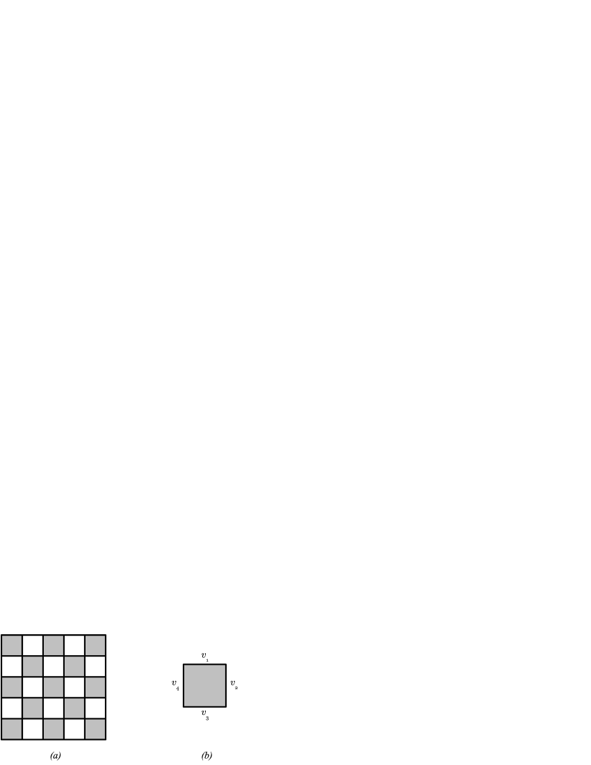
Figure 1: a) The square lattice with the checkerboard couplings shown in b).

Now let $G$ be the square lattice, and choose the 4-edge basis $B$ with couplings $\{v_{1},v_{2},v_{3},v_{4}\}$ shown in Figure 1b. We choose the checkerboard embedding of $B$ in $G$ shown in Figure 1a. The contraction-deletion definition [1] amounts to assuming that the critical polynomial $P_{B}(q,v)$ satisfies the same identity as (8) for any edge $e\in B$. Performing the deletion-contraction of the edge with weight $v_{4}$ we thus obtain

$$P_{B}(q,\{v_{1},v_{2},v_{3},v_{4}\})=v_{4}P_{B^{\rm tri}}(q,\{v_{1},v_{2},v_{3}\})+P_{B^{\rm hex}}(q,\{v_{1},v_{2},v_{3}\})\,.$$ (9)

In the first (contracted) term the embedded basis now spans the triangular lattice, so we can insert the known exact result

$$P_{B^{\rm tri}}(q,\{v_{1},v_{2},v_{3}\})=v_{1}v_{2}v_{3}+v_{1}v_{2}+v_{2}v_{3}+v_{3}v_{1}-q\,,$$ (10)

that generalises (3). In the second (deleted) term we recover the hexagonal lattice, for which the exact result generalising (4) reads

$$P_{B^{\rm hex}}(q,\{v_{1},v_{2},v_{3}\})=v_{1}v_{2}v_{3}-q(v_{1}+v_{2}+v_{3})-q^{2}\,.$$ (11)

Inserting (10)–(11) into (9) we arrive at the desired critical polynomial

$$P_{B}(q,\{v_{1},v_{2},v_{3},v_{4}\}) = v_{1}v_{2}v_{3}v_{4}+v_{2}v_{3}v_{4}+v_{1}v_{3}v_{4}+v_{1}v_{2}v_{4}+v_{1}v_{2}v_{3}$$ (12)

$$-q(v_{1}+v_{2}+v_{3}+v_{4})-q^{2}\,.$$

Note that the expression $P_{B}(q,\{v_{1},v_{2},v_{3},v_{4}\})=0$ coincides with a result derived by Wu [18] using a different method (and a homogeneity assumption).

Critical polynomials $P_{B}(q,v)$ defined in this way are unique, that is, they are a property only of the basis $B$ and the way in which $B$ is embedded in the infinite lattice $G$. In particular, $P_{B}(q,v)$ is independent of the order in which edges are contracted-deleted [15].

In the particular case considered above, (12) actually provides the exact critical manifold of the square lattice with checkerboard couplings [13]. However, as mentioned in the Introduction and discussed in details in [1], in general we only recover an approximation to the critical manifold, that converges to the true critical manifold upon letting the size of $B$ go to infinity (at finite aspect ratio). How close one can get to $v_{c}$ is thus limited by one’s ability to actually compute the polynomial on large $B$. In [1], a computer program was used to perform the contraction-deletion algorithm on various bases for the kagome lattice. However, this algorithm is exponential in the number of edges in $B$, and the upper limit of feasibility was $36$ edges.

Below, we present an alternative definition of $P_{B}(q,v)$ in terms of probabilities of events on $B$. This permits use of a transfer matrix approach, a much more efficient algorithm that is, roughly speaking, exponential only in the number of vertices across a horizontal cross-section of $B$. By these means, we will be able to compute critical polynomial on the $(4,8^{2})$, kagome, and $(3,12^{2})$ lattices for bases of up to respectively 96, 162, and 243 edges. These three lattices are shown in Figure 2. We note that in parts of sections 2–3 we will present material that has been discussed for $q=1$ in our previous work on percolation [20]. Many of these concepts are identical or only slightly modified in the Potts generalization, but for the sake of completeness we explain these in full below, reproducing some passages verbatim from [20].

Figure 2: a) the kagome lattice; b) the $(4,8^{2})$ lattice; c) the $(3,12^{2})$ lattice.

2.1 Alternative definition

According to (1), the probability of any event on the finite graph $B$ is proportional to a sum of terms of the type $\left(\prod_{i\in A}v_{i}\right)q^{k(A)}$, where $A$ are some subsets of the edges in $B$ describing which edges need to be present in order to realise the event. We are here interested in the probabilistic, geometrical interpretation of the critical polynomials $P_{B}(q,v)$ in terms of such events. But to discuss this, we will first need some definitions.

The infinite lattice $G$ is partitioned into identical subgraphs $B$, and we assume that each is in the same edge-state. We are interested in the global connectivity properties of the system. If, given any two copies of the basis, $B_{1}$ and $B_{2}$, separated by an arbitrary distance, it is possible to travel from $B_{1}$ to $B_{2}$ along an open path, then we say that there is an infinite two-dimensional (2D) cluster in the system. We denote the weight of this event $W(2D;B)$. On the other hand, if it is not possible to connect any non-neighbouring $B_{1}$ and $B_{2}$, then there are no infinite clusters in the system, a situation whose weight we write as $W(0D;B)$. The third possibility is that some arbitrarily separated $B_{1}$ and $B_{2}$ are connected, but not all, indicating the presence of infinite one-dimensional (1D) paths (or filaments), and we denote the corresponding weight $W(1D;B)$.

We have found that all the (inhomogeneous) critical polynomials $P_{B}(q,\{v\})$ that we have computed using the contraction-deletion definition can be rewritten very simply as

$$P_{B}(q,\{v\})=W(2D;B)-q\,W(0D;B)\,.$$ (13)

Despite its apparent simplicity, eq. (13) is the main result of this paper.

To make completely clear the meaning of (13) we need to discuss two important points.

First, one may wish to think of the quantities $W(2D;B)$ and $W(0D;B)$ appearing on the left-hand side of (13) as describing the probabilities of the events defined above. However, since the critical manifold is found from $P_{B}(q,\{v\})=0$, normalisation issues are not important. It is thus more convenient to define the $W$ with a normalisation that reflects that of the partition function (1).

Second, we have to be precise about how the powers of $q$ are computed. In Figures 3–4 we show several examples of embedded bases $B$. Recall that $G$ is obtained by tiling the two-dimensional space with copies of $B$. The vertices at the tile boundaries are shared among two different copies of $B$; we call those shared vertices the terminals of $B$. The embedding can be visualised by pairing the terminals two by two (shown as matching shapes in Figures 3–4). This means that in the embedding a given terminal of one copy of the basis $B_{1}$ is identified with the matching terminal of another copy of the basis $B_{2}$. In other words, $B_{1}$ and $B_{2}$ are glued along matching terminals. Let now $A$ be a subset of edges of $B$ describing a certain event, which we classify as 2D, 1D or 0D as above. The weight in the corresponding $W$ of the event described by $A$ is defined as

$$\left(\prod_{i\in A}v_{i}\right)q^{k(A)-1}\,,$$ (14)

where $k(A)$ is the number of connected components induced by $A$ in the (generally non-planar) graph obtained from $B$ by identifying the matching terminals as in the definition of the embedding. Note also that since $k(A)\geq 1$, we have chosen the power of $q$ appearing in (14) as $k(A)-1$ rather than $k(A)$. With this convention we avoid having an overall factor of $q$ in (13).

With the definitions (13)–(14) the critical polynomial coincides with that defined in [1]. That the probabilistic and contraction-deletion definitions produce the same polynomial can be seen as follows. First, we note that the probabilities $W(2D)$ and $W(0D)$ separately satisfy the contraction-deletion identity. This is because these quantities are just restricted partition functions and will therefore satisfy the same contraction-deletion property as does the full partition function. In the definition made in [1], contraction-deletion was used as a recurrence to reduce any basis to a number of three-terminal cases, for which the exact solvability criterion for 3-uniform hypergraphs was inserted as an initial condition. That latter criterion reads [21] $qA-C=0$, where $A$ and (resp. $C$) denotes the weight of all three vertices surrounding a hyper-edge being unconnected (resp. connected). It is easy to see that Eqs. (13)–(14) precisely reproduce this initial condition. Since the recurrence relation (i.e., contraction-deletion) is also identical for the two definitions, it follows that they produce the same critical polynomial for any choice of the basis $B$.

To see the definitions (13)–(14) at work, we consider again the 4-edge checkerboard example of Figure 1. We have

$$W(2D;B) = v_{1}v_{2}v_{3}v_{4}+v_{2}v_{3}v_{4}+v_{1}v_{3}v_{4}+v_{1}v_{2}v_{4}+v_{1}v_{2}v_{3}\,,$$ (15)

$$W(1D;B) = v_{1}v_{2}+v_{1}v_{3}+v_{1}v_{4}+v_{2}v_{3}+v_{2}v_{4}+v_{3}v_{4}\,,$$ (16)

$$W(0D;B) = v_{1}+v_{2}+v_{3}+v_{4}+q\,.$$ (17)

Inserting this in (13) indeed reproduces (12).

Finally we note that for the the special case of percolation, the probabilistic definition of $P_{B}(q,v)$ has already appeared in [20]. The results reported here reduce to those of [20] upon setting $q=1$ and $v_{i}=\frac{p_{i}}{1-p_{i}}$, where $p_{i}$ is the probability of edge $i$ being open.

2.2 Bases and embeddings

As mentioned above, one advantage of the redefinition (13) is that we may now use a transfer matrix to compute the critical polynomials on much larger bases than was possible using contraction-deletion. Below we give the details of this approach (section 3) and report the results for various lattices (section 4).

But first we discuss more carefully the bases that we have considered. We are mainly interested in families of bases whose size can be modulated by varying one or more integer parameters. This will in particular allow us to study the size dependence of the resulting $p_{c}$.

2.2.1 Square bases

An example of a square basis $B$ is shown in Figure 3. We recall that the embedding is visualised by pairing the terminals two by two (shown as matching shapes in Figure 3). The embedded basis in Figure 3a is the immediate generalisation of the checkerboard example shown in Figure 1, and we refer to this as the straight embedding.

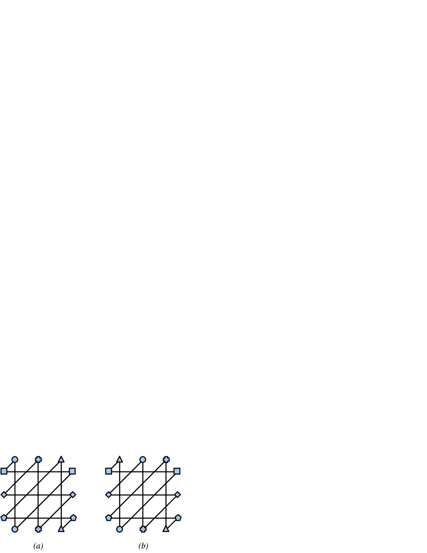
Figure 3: $3\times 3$ square bases for the kagome lattice with: a) straight embedding, b) a twisted embedding.

A variation of the straight embedding is to shift cyclically the vertices along one of the sides of the square before gluing them to those of the opposing side; we call this a twisted embedding. By reflection symmetry, shifting cyclically $k$ steps to the right or to the left produces identical results. There are thus in general $1+\lfloor n/2\rfloor$ inequivalent twists, corresponding to $k=0,1,\ldots,\lfloor n/2\rfloor$. In practice we have found that for some—but not all—lattices the cases $(n,k)=(2,0)$ and $(n,k)=(2,1)$ produce the same critical polynomial. But in general the twisting does change the critical polynomial, as we shall see below.

A square basis $B$ of size $n\times n$ has $n$ terminals on each of the four sides of the square. The number of vertices and edges in $B$ are both proportional to $n^{2}$. In the vertex count, each terminal counts for $1/2$ only, since it is shared among two copies of the basis. Thus, the square basis for the kagome lattice shown in Figure 3 has $6n^{2}$ edges and $3n^{2}$ vertices.

One can obviously generalise this construction to rectangular bases of size $n\times m$. For $n=m$ one recovers a square basis. For $n\neq m$ the twists along the $n$ and $m$ directions are no longer equivalent.

2.2.2 Hexagonal bases

When the lattice $L$ has a 3-fold rotational symmetry, one can define as well a hexagonal embedding. Examples of this are shown in Figure 4. Each of the six sides of the hexagon now supports $n$ terminals. Note that it is not possible to twist the hexagonal bases, since only the straight embedding produces a valid tiling of two-dimensional space.

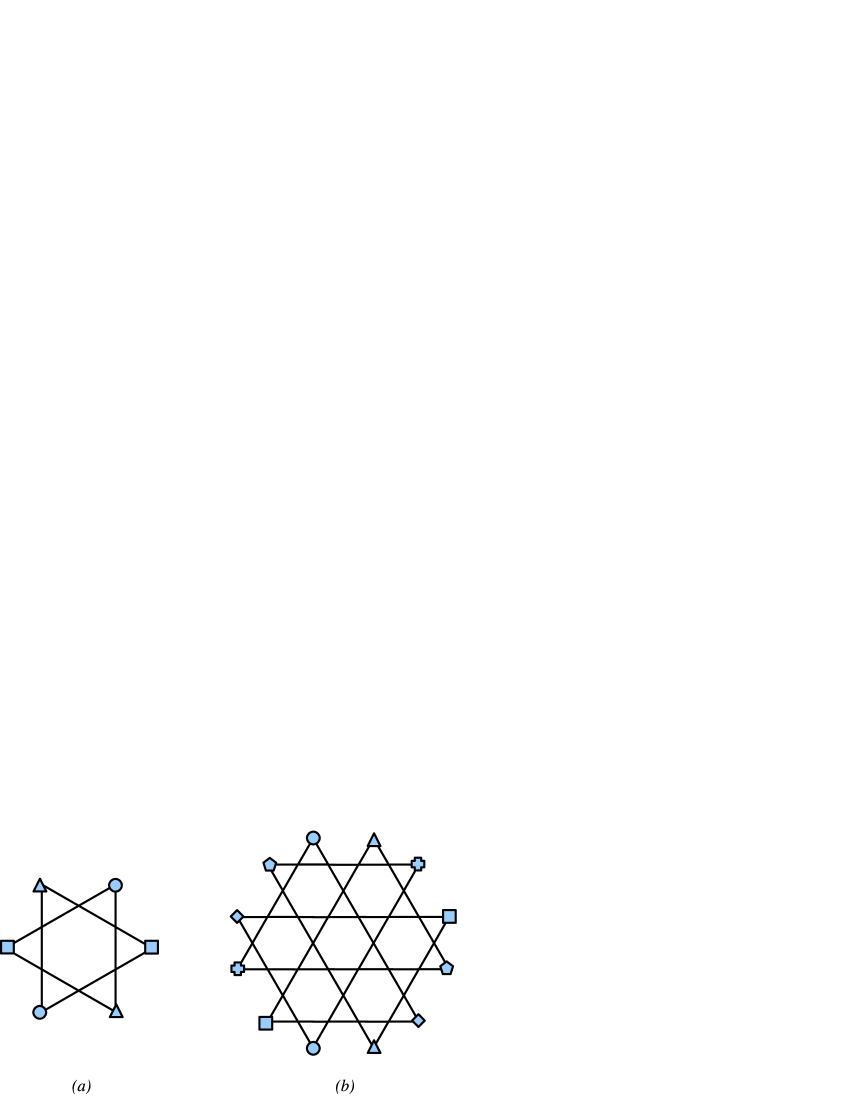
Figure 4: Hexagonal bases for the kagome lattice with a) $n=1$, and b) $n=2$.

An advantage of hexagonal bases over the square bases is that they have a lower ratio of terminals to edges. For example, on the kagome lattice one has now $6n$ terminals, $9n^{2}$ vertices and $18n^{2}$ edges. This is useful because the number of terminals is the limiting factor in the transfer matrix computation while the accuracy of the critical point estimates increases with the number of edges.

Another advantage is that the hexagonal basis is designed to respect the 3-fold rotational symmetry of the lattice. Thus, for lattices having this symmetry—such as the kagome and $(3,12^{2})$ lattices—we expect the hexagonal basis to yield better accuracy than the square basis for a given number of edges. We shall come back to this point in section 4.

Note that one can extend this construction to generalised hexagonal bases with $2(n_{1}+n_{2}+n_{3})$ terminals, where each pair of opposing sides of the hexagon supports $n_{i}$ terminals $(i=1,2,3)$. The special case with one of the $n_{i}=0$ reproduces the rectangular bases.

3 Transfer matrix

The weights $W(2D;B)$ and $W(0D;B)$ entering the definition (13) of the critical polynomial can be computed from a transfer matrix construction along the lines of Ref. [22]. First notice that each state of the edges within the basis $B$ induces a set partition among the terminals; each part (or block) in the partition consists of a subset of terminals that are mutually connected through paths of open edges. The key idea is to first compute the weights of all possible partitions. One next groups the partitions according to their 2D, 1D or 0D nature in order to evaluate (13).

With $N$ terminals, the number of partitions respecting planarity is given by the Catalan number

$$C_{N}=\frac{1}{N+1}{2N\choose N}\,.$$ (18)

For example, the $C_{3}=5$ planar partitions of the set $\{1,2,3\}$ are denoted

$$(1)(2)(3)\,,\quad(12)(3)\,,\quad(13)(2)\,,\quad(1)(23)\,,\quad(123)\,,$$ (19)

where the elements belonging to the same part are grouped inside parentheses.

The dimension of the transfer matrix is thus $C_{N}$, and both time and memory requirements are proportional to this number. Asymptotically we have $C_{N}\sim 4^{N}$ for $N\gg 1$. Taking as an example the kagome lattice with the $n\times n$ square basis, the time complexity of the transfer matrix method is then $\sim 4^{4n}=2^{8n}$. This can be compared to the contraction-deletion method, whose number of recursive calls is $\sim 2^{6n^{2}}$.

3.1 Square bases

Our transfer matrix construction is most easily explained on a specific example. So consider the kagome lattice with the $n\times n$ square basis; the case $n=3$ is shown in Figure 5.

Figure 5: Transfer matrix construction for the kagome lattice on an $n\times n$ square basis, here with $n=3$. The operator ${\sf B}_{i}$ adds six edges to the lattice.

The transfer matrix ${\sf T}$ constructs the lattice from the bottom to the top, while keeping track of the Boltzmann weight of each partition of the terminals. The bottom terminals are denoted $1,2,\ldots,2n$ and the top terminals $1^{\prime},2^{\prime},\ldots,2n^{\prime}$. At the beginning of the process the top and bottom are identified, so the initial state $|{\rm i}\rangle$ on which ${\sf T}$ acts is the partition $(1\,1^{\prime})(2\,2^{\prime})\cdots(2n\,2n^{\prime})$ with weight $1$.

We now define two kinds of operators acting on a partition [24]:

• The join operator ${\sf J}_{i}$ amalgamates the parts to which the top terminals $i^{\prime}$ and $i^{\prime}+1$ belong. In particular, on partitions in which those two terminals already belong to the same part, ${\sf J}_{i}$ acts as the identity operator ${\sf I}$. Note that if some parts contain both bottom and top terminals, the action of ${\sf J}_{i}$ can also affect the connections among the bottom terminals.

• The detach operator ${\sf D}_{i}$ detaches the top terminal $i^{\prime}$ from its part and transforms it into a singleton in the partition. But if that terminal was already a singleton, ${\sf D}_{i}$ acts as $q\,{\sf I}$. The reason for the factor of $q$ is that a detached singleton amounts to a connected component being “seen for the last time”, and ${\sf D}_{i}$ should then apply the corresponding weight appearing in (14).

From these two basic operators and the identity operator ${\sf I}$ we now define an operator

$${\sf H}_{i}={\sf I}+v{\sf J}_{i}$$ (20)

that adds a horizontal edge to the lattice. The word “horizontal” refers to a drawing of the lattice where the top terminals $i^{\prime}$ and $i^{\prime}+1$ are horizontally aligned; otherwise the edge would be better described as “diagonal”. Note that ${\sf H}_{i}$ attaches a weight $1$ (resp. $v$) to a closed (resp. open) horizontal edge, as required. Similarly we define

$${\sf V}_{i}=v{\sf I}+{\sf D}_{i}$$ (21)

that adds a vertical edge between $i^{\prime}$ and $i^{\prime\prime}$, where $i^{\prime}$ (resp. $i^{\prime\prime}$) denotes the corresponding top terminal before (resp. after) the action of ${\sf V}_{i}$. To simplify the notation, it is convenient to assume that following the action of ${\sf V}_{i}$ we relabel $i^{\prime\prime}$ as $i^{\prime}$. The word “vertical” refers to a drawing of the lattice where $i^{\prime}$ and $i^{\prime\prime}$ are vertically aligned.

The fundamental building block of the lattice shown on the right of Figure 5 is then constructed by the composite operator

$${\sf B}_{i}={\sf H}_{i}{\sf V}_{i}{\sf H}_{i}{\sf D}_{i+1}{\sf H}_{i}{\sf V}_{i}{\sf H}_{i}\,,\qquad\mbox{Kagome lattice}$$ (22)

where the operators here and elsewhere should be understood as acting in order from right to left. The whole lattice $B$ is finally obtained by adding successive rows (for clarity shown in alternating hues on the left of Figure 5) of ${\sf B}_{i}$. The transfer matrix then reads

$${\sf T}=\prod_{y=1}^{n-1}\prod_{x=1}^{y}{\sf B}_{n-y-1+2x}\times\prod_{y=1}^{n}\prod_{x=0}^{n-y}{\sf B}_{y+2x}$$ (23)

and the final state

$$|{\rm f}\rangle={\sf T}|{\rm i}\rangle$$ (24)

contains all possible partitions among the $4n$ terminals along with their respective Boltzmann weights.

The final state $|{\rm f}\rangle$ contains all the information necessary to extract $P_{B}(q,v)$, and the remainder of section 3 explains how this is done. But first we describe how to modify the transfer matrix formalism just described to accommodate other lattices (section 3.1.1) and hexagonal bases (section 3.2). Then, in section 3.3, we show how to determine which of the states in $|{\rm f}\rangle$ contribute to the weights $W(2D;B)$ and $W(0D;B)$ appearing in (13).

Finally, each contributing state needs to be counted with the correct weight (14). The powers of $v$ are unproblematic and have been explicitly accounted for in (20)–(21). The contributions to $q^{k(A)-1}$ originating from connected components not containing any terminal of $B$ have been accounted for in the above definition of ${\sf D}_{i}$. It remains to explain how to count the connected components containing at least one terminal; this is the subject of section 3.4.

3.1.1 Other lattices

The extension of the transfer matrix formalism to the other lattices considered in this paper is very simple: it suffices to change the definition of the operator ${\sf B}_{i}$, while leaving the remainder of the construction unchanged.

Figure 6: Transfer matrix construction for the $(4,8^{2})$ lattice on an $n\times n$ square basis, here with $n=3$. The operator ${\sf B}_{i}$ adds six edges to the lattice.

The square basis for the $(4,8^{2})$ lattice is shown in Figure 6. Its fundamental building block now has the expression

$${\sf B}_{i}={\sf H}_{i}{\sf V}_{i}{\sf V}_{i+1}{\sf H}_{i}{\sf V}_{i}{\sf V}_{i+1}\,,\qquad\mbox{$(4,8^{2})$ lattice.}$$ (25)

Figure 7: Transfer matrix construction for the $(3,12^{2})$ lattice on an $n\times n$ square basis, here with $n=3$. The operator ${\sf B}_{i}$ adds nine edges to the lattice.

As a last example, consider the $(3,12^{2})$ lattice with the square basis depicted in Figure 7. We find in this case

$${\sf B}_{i}={\sf H}_{i}{\sf V}_{i}{\sf H}_{i}{\sf V}_{i}{\sf D}_{i+1}{\sf H}_{i}{\sf V}_{i}{\sf H}_{i}{\sf V}_{i}{\sf V}_{i+1}\,,\qquad\mbox{$(3,12^{2})$ lattice.}$$ (26)

3.2 Hexagonal bases

Because of their 3-fold rotational symmetry, it is also interesting to study the kagome and $(3,12^{2})$ lattice with a hexagonal basis. We now describe how to adapt the transfer matrix construction to this case.

Figure 8: Kagome lattice on a hexagonal basis of size $n$, here with $n=3$. The operator ${\sf B}_{i}$ adds six edges to the lattice, while the left and right boundary operators, ${\sf L}_{i}$ and ${\sf R}_{i}$, each add three.

Consider as an example the kagome lattice with the hexagonal basis of size $n$; the case $n=3$ is shown in Figure 8. There are now $6n$ terminals. Those on the two bottom sides (resp. the two top sides) of the hexagon are labelled $1,2,\ldots,2n$ (resp. $1^{\prime},2^{\prime},\ldots,2n^{\prime}$), just as in the case of the square basis. We describe below how the remaining terminals on the left and right sides of the hexagon are to be handled. The transfer matrix ${\sf T}$ still constructs the lattice from the bottom to the top.

The expression for the building block ${\sf B}_{i}$ now needs some modification, since the orientation of the bow tie motif with respect to the transfer direction (invariably upwards) has been changed. One easy option would be to handle the centre of the bow tie as an extra point—we would then label the three points $i$, $i+1$ and $i+2$)—and use the expression ${\sf B}_{i}={\sf D}_{i+1}{\sf H}_{i+1}{\sf H}_{i}{\sf V}_{i+2}{\sf V}_{i}{\sf H}_{i+1}{\sf H}_{i}$. It is however more efficient to avoid introducing the centre point into the partition (and keep the usual labelling $i$, $i+1$ as shown on the right of Figure 8). The expression for ${\sf B}_{i}$ can then be found by computing the final state (24) for the $1\times 1$ square basis and rotating the labels (we denote here $j=i+1$):

$${\sf B}_{i} = (v^{6}+6v^{5}+9v^{4})(iji^{\prime}j^{\prime})+(2v^{4}+6v^{3}+qv^{2})(ii^{\prime})(jj^{\prime})$$ (27)

$$+ (v^{4}+3v^{3})\big{[}(i)(ji^{\prime}j^{\prime})+(j)(ii^{\prime}j^{\prime})+(i^{\prime})(ijj^{\prime})+(j^{\prime})(iji^{\prime})\big{]}$$

$$+ (v^{3}+5v^{2}+qv)\big{[}(ii^{\prime})(j)(j^{\prime})+(i)(i^{\prime})(jj^{\prime})\big{]}+(4v+q)(i)(j)(i^{\prime})(j^{\prime})$$

$$+ v^{2}\left[(i)(j)(i^{\prime}j^{\prime})+(ij)(i^{\prime})(j^{\prime})+(i)(i^{\prime}j)(j^{\prime})+(i^{\prime})(ij^{\prime})(j)\right]\,.$$

where a bracketed operator, for example $(ii^{\prime})(jj^{\prime})$, creates a bow-tie between $i$ and $j$ with the indicated partition of its four bounding vertices. On the boundary of the hexagon we need the further operators

$${\sf L}_{i} = {\sf H}_{i}{\sf V}_{i+1}{\sf H}_{i}\,,$$ (28)

$${\sf R}_{i} = {\sf H}_{i}{\sf V}_{i}{\sf H}_{i}\,.$$ (29)

The transfer matrix that builds the whole hexagon then reads

$${\sf T} = \prod_{y=1}^{n-1}\prod_{x=1}^{y}{\sf B}_{n-y-1+2x}$$ (30)

$$\times \prod_{y=1}^{n}\left(\prod_{x=1}^{n}{\sf B}_{2x-1}\times{\sf L}_{0}\prod_{x=1}^{n-1}{\sf B}_{2x}\times{\sf R}_{2n}\right)\times\prod_{y=1}^{n}\prod_{x=0}^{n-y}{\sf B}_{y+2x}\,.$$

Regarding the handling of the boundary points, a small remark is in order. In (30) these have been denoted simply $0$ (on the left) and $2n+1$ (on the right). In the initial state $|{\rm i}\rangle$, both $0$ and $2n+1$ are singletons. After each factor in the middle product over $y$ the two boundary labels have to be stored, so that in the final state (24) the partitions indeed involve all $6n$ terminals. To avoid introducing a cumbersome notation, we understand implicitly that this storing is performed when expanding the product (30).

3.2.1 Other lattices

The $(3,12^{2})$ lattice can be handled similarly by rotating ${\sf B}_{i}$ shown in the right part of Figure 7 through angle $\pi/2$ clockwise. The left (resp. right) boundary operator ${\sf L}_{i}$ (resp. ${\sf R}_{i}$) then consists of the four rightmost (resp. five leftmost) edges in the rotated ${\sf B}_{i}$. Explicitly we find

$${\sf B}_{i} = (v^{9}+6v^{8}+9v^{7})(iji^{\prime}j^{\prime})+(v^{7}+3v^{6})\left[(iji^{\prime})(j^{\prime})+(iji^{\prime})(j)\right]$$

$$+ (v^{8}+7v^{7}+(12+q)v^{6}+3qv^{5})\left[(i)(ji^{\prime}j^{\prime})+(i^{\prime})(ijj^{\prime})\right]$$

$$+ (v^{8}+8v^{7}+(15+2q)v^{6}+7qv^{5}+q^{2}v^{4})(ii^{\prime})(jj^{\prime})$$

$$+ (3v^{6}+(11+q)v^{5}+6qv^{4}+q^{2}v^{3})(ii^{\prime})(j)(j^{\prime})$$

$$+ (3v^{7}+(27+q)v^{6}+(56+21q)v^{5}+(63q+7q^{2})v^{4}$$

$$+(33q^{2}+q^{3})v^{3}+9q^{3}v^{2}+q^{4}v)(i)(i^{\prime})(jj^{\prime})$$

$$+ (v^{6}+4v^{5}+qv^{4})\left[(i)(j)(i^{\prime}j^{\prime})+(ij)(i^{\prime})(j^{\prime})+(i)(i^{\prime}j)(j^{\prime})+(i^{\prime})(ij^{\prime})(j)\right]$$

$$+ (8v^{5}+(40+5q)v^{4}+(48q+q^{2})v^{3}+27q^{2}v^{2}+8q^{3}v+q^{4})(i)(j)(i^{\prime})(j^{\prime})$$

along with

$${\sf L}_{i} = (v^{4}+3v^{3})(ijj^{\prime})+(v^{3}+4v^{2}+qv)(i)(jj^{\prime})$$ (32)

$$+ v^{2}\left[(ij)(j^{\prime})+(ij^{\prime})(j)\right]+(3v+q)(i)(j)(j^{\prime})$$

and

$${\sf R}_{i} = (v^{5}+3v^{4})(ii^{\prime}j)+(v^{4}+4v^{3}+qv^{2})\left[(ij)(i^{\prime})+(i)(i^{\prime}j)\right]$$ (33)

$$+ v^{3}(ii^{\prime})(j)+(v^{3}+8v^{2}+5qv+q^{2})(i)(j)(i^{\prime})\,.$$

With these expressions for ${\sf B}_{i}$, ${\sf L}_{i}$ and ${\sf R}_{i}$, the transfer matrix is still given by (30).

3.3 Distinguishing 2D, 1D and 0D partitions

We now explain how each partition entering the final state (24) can be assigned the correct homotopy (0D, 1D or 2D) in order to make possible the application of the main result (13). The definition of homotopy that we have given in section 2.1 is not very practical, because it refers to the connectivity properties between two arbitrarily separated copies of the basis, $B_{1}$ and $B_{2}$. The purpose of this section is to provide an operational determination of the homotopy using just intrinsic properties of $B$.

Each partition of the set of $N$ terminals can be represented as a planar hypergraph on $N$ vertices, where each part of size $k>1$ in the partition corresponds to a hyperedge of degree $d=k-1$ in the hypergraph. Because of the planarity we can obtain yet another representation as an ordinary graph on $2N$ vertices with precisely $N$ ordinary ($d=1$) edges. We now detail this construction, which is completely analogous to a well-known [25] equivalence for the partition function of the Potts model defined on a planar graph $G$ that can be represented, on the one hand, in terms of Fortuin-Kasteleyn clusters [5] on $G$ and, on the other hand, as a loop model on the medial graph ${\cal M}(G)$.

The hypergraph can be drawn inside the frame (the outer boundary of the shaded areas in Figures 5 and 8) on which the $N$ terminals live. Here we give a few examples:

Now place a pair of points slightly shifted on either side of each of the $N$ terminals. Draw $N$ edges between these $2N$ points by “turning around” the hyperedges and isolated vertices of the hypergraph. We shall refer to this as the surrounding graph. For each of the above examples this produces:

The embedding of $B$ is defined by identifying points on opposing sides of the frame (to produce the twisted embeddings we further shift the points on one of the sides cyclically before imposing the identification). Let $\ell$ be the number of loops in the surrounding graph. The partition is of the 1D type if and only if one or more of these loops is non-homotopic to a point. To determine whether this is the case it suffices to “follow” each loop until one comes back to the starting point, and determine whether the total signed displacement in the $x$ and $y$ directions is non-zero. Using this method one sees that the middle partition in the above three examples is of the 1D type.

If all loops on the surrounding graph have trivial homotopy, one can use the Euler relation to determine whether the partition is of the 0D or 2D type. Namely, let $E$ be the sum of all degrees of the hyperedges in the hypergraph; let $C$ (resp. $V$) be the number of connected components (resp. vertices) in the hypergraph after the identification of opposing sides. Then the combination

$$\chi=E+2C-V-\ell$$ (34)

equals 0 (resp. 2) if the partition is of the 0D (resp. 2D) type.

For instance, for the leftmost example we have $E=3+1+1=5$, $C=1$, $V=6$, and $\ell=1$, whence $\chi=0$. And for the rightmost example one finds $E=5+1=6$, $C=2$, $V=6$, and $\ell=2$, whence $\chi=2$.

3.4 Number of connected components containing a terminal

To finish the computation of the factor $q^{k(A)-1}$ in (14), it remains to count the number of connected components (minus one) containing at least one terminal. The terminals are nothing but the points in the partition describing the final state (24). But before counting we need to identify the matching terminals, as shown in Figures 3–4.

The algebraic formulation of this counting procedure is simple. Let the number of terminals be $2N$, with $N=2n$ (resp. $N=3n$) for the square (resp. hexagonal) bases. Matching terminals are labelled $\{i_{k},j_{k}\}$, for $k=1,2,\ldots,N$. The operator ${\sf J}$ identifying all matching pairs of terminals is then expressed in terms of join operators ${\sf J}_{ij}$ as

$${\sf J}=\prod_{k=1}^{N}{\sf J}_{i_{k},j_{k}}\,.$$ (35)

To multiply the weights by the correct power of $q$ we finally apply

$${\sf D}=q^{-1}\prod_{k=1}^{N}{\sf D}_{i_{k}}{\sf D}_{j_{k}}\,.$$ (36)

More precisely, let $|{\rm f}\rangle_{2D}$ denote the terms in the final state (24) whose partitions are of 2D topology. Then

$${\sf D}{\sf J}|{\rm f}\rangle_{2D}=W(2D;B)\,(i_{1})(i_{2})\cdots(i_{N})(j_{1})(j_{2})\cdots(j_{N})\,,$$ (37)

i.e., one of the weights needed in (13) times the all-singleton state. We similarly obtain $W(0D;B)$ from $|{\rm f}\rangle_{0D}$.

Let us illustrate this procedure by a small example. The final state $|{\rm f}\rangle$ corresponding to the $1\times 1$ square basis for the kagome lattice can be read directly off the right-hand side of (27). The unique partition having 2D topology is $(iji^{\prime}j^{\prime})$. The partitions having 0D topology are $(ii^{\prime})(j)(j^{\prime})$, $(i)(i^{\prime})(jj^{\prime})$, $(i)(j)(i^{\prime})(j^{\prime})$, $(i)(j)(i^{\prime}j^{\prime})$ and $(ij)(i^{\prime})(j^{\prime})$. The corresponding terms in the sum (27) then define $|{\rm f}\rangle_{2D}$ and $|{\rm f}\rangle_{0D}$. Applying the operator ${\sf D}{\sf J}$ as above, we infer that

$$W(2D;B) = v^{6}+6v^{5}+9v^{4}\,,$$ (38)

$$W(0D;B) = 2\times(v^{3}+5v^{2}+qv)+(4v+q)\times q+2\times v^{2}\,.$$ (39)

According to (13) the critical polynomial is then

$$P_{B}(q,v)=v^{6}+6v^{5}+9v^{4}-2qv^{3}-12qv^{2}-6q^{2}v-q^{3}\,.$$ (40)

The expression $P_{B}(q,v)=0$ is precisely the approximation to the kagome-lattice critical manifold found by Wu [18].

4 Results

Using the transfer matrix approach we have computed the critical polynomials $P_{B}(q,v)$ for the kagome, $(4,8^{2})$ and $(3,12^{2})$ lattices; see Figure 2. With the $n\times n$ square bases, the computations were possible for $n\leq 4$, both with straight and twisted embeddings. This is a considerable improvement over the contraction-deletion method, where the $2\times 3$ rectangular basis (with 36 edges for the kagome lattice) was the furthest we could go [1]. With the hexagonal bases, the transfer matrix computations were possible for $n\leq 2$. For selected integer values of $q$, the case $n=3$ was within reach as well, albeit with large parallel computations; the $n=3$ results for percolation ($q=1$) have been reported in [20].

The critical polynomials that we have obtained are very large. To be precise, let $|V|$ (resp. $|E|$) denote the number of vertices (resp. edges) in the basis, with the convention that a pair of matching terminals counts as a single vertex. Then $P_{B}(q,v)$ is a polynomial of degree $|V|$ in the $q$ variable, and of degree $|E|$ in the $v$ variable, with very large integer coefficients (more than 100 digits in some cases). Obviously it is out of the question to make these polynomials appear in print. However, all the polynomials are collected in the text file JS12.m which is available in electronic form as supplementary material to this paper. The printed version contains only selected values of the roots $v_{c}$, rounded to 15 digit numerical precision, and plots of the curves $P_{B}(q,v)=0$ in the real $(q,v)$ plane (see section 5).

In this section we analyse the approximations to the critical temperatures, $v_{c}$, obtained by solving $P_{B}(q,v)=0$ in the ferromagnetic regime ($v>0$) for selected integer values of $q$ of practical interest, namely $q=2,3,4$. The corresponding results for $q=1$ have already appeared in [20]. Then, in section 5, we extend the discussion to the full phase diagram in the real $(q,v)$ plane.

4.1 Kagome lattice

For the kagome lattice, we considered two families of bases: square (see section 2.2.1) and hexagonal (see section 2.2.2).

4.1.1 Square bases

The $n\times n$ square bases with straight and twisted embeddings are shown in Figure 3. They contain $|V|=3n^{2}$ vertices and $|E|=6n^{2}$ edges. We have obtained the critical polynomials for $n\leq 4$ and twist $k\leq\lfloor n/2\rfloor$.

For $q=2$ all those polynomials factorise, shedding the small factor

$$v^{4}+4v^{2}-8v-8\,.$$ (41)

This factorisation is expected [1], since the Ising model is exactly solvable. The unique positive root of (41) reads

$$v_{c}=\sqrt{3+2\sqrt{3}}-1=1.542\,459\,756\cdots\,,$$ (42)

in agreement with the exact solution [26].

$n$	twist	$v_{c}$ for $q=3$	$v_{c}$ for $q=4$
1	0	1.876 269 208 345 761	2.155 842 236 513 638
2	0	1.876 439 754 302 881	2.156 207 452 990 795
	1	1.876 439 754 302 881	2.156 207 452 990 795
3	0	1.876 456 916 196 415	2.156 247 598 338 124
	1	1.876 456 775 276 423	2.156 247 104 437 170
4	0	1.876 458 994 003 462	2.156 252 880 154 217
	1	1.876 458 930 268 948	2.156 252 686 506 350
	2	1.876 458 896 874 446	2.156 252 553 917 008
Final		1.876 459 0  (5)	2.156 253  (1)
Numerics	Ref. [1]	1.876 459  (2)	2.156 252 (2)
	Ref. [27]	1.876 458  (3)	2.156 20 (5)

Table 1: Predictions for the critical temperature $v_{c}$ of the Potts model on the kagome lattice, obtained from the $n\times n$ square bases with various twists. Extrapolation to $n\to\infty$ leads to the final results quoted. For comparison we show two sets of recent numerical results [1, 27].

The positive roots of $P_{B}(q,v)$ for $q=3$ and $q=4$ are given in Table 1. Note that the results for $(n,k)=(2,0)$ and $(2,1)$ are identical for this lattice; but otherwise the critical polynomial does depend on $k$. Based on the results for finite $n$ we suggest the final values shown in the bottom of Table 1. They are compatible with the results for the largest ($n=4$) basis for any $k$, and the indicative error bar has been obtained by comparing the variation of the results for various twists, and by a crude analysis of the the finite-size effects in $n$ with zero twist. Our final values agree with—and are marginally more precise than—two sets of recent numerical results, obtained respectively from the crossings of effective critical exponents [27] and from the maximum of the effective central charge [1].

4.1.2 Hexagonal bases

The hexagonal bases of size $n$ are shown in Figure 4. They contain $|V|=9n^{2}$ vertices and $|E|=18n^{2}$ edges. As discussed in section 2.2.2, these bases better respect the rotational symmetry of the lattice, and hence we expect the results to be more precise than those with the square bases for a given number of edges. We have obtained the full critical polynomials $P_{B}(q,v)$ for $n\leq 2$. For $n=3$ we have also obtained polynomials $P_{B}(q_{0},v)$ in the $v$ variable for the integer values $q_{0}=3$ and 4 (see also [20] for the case $q_{0}=1$).

For $q=2$ the polynomials again yield the exact result, since they invariably contain the factor (41). Results for $q=3$ and $q=4$ are given in Table 2.

$n$	$v_{c}$ for $q=3$	$v_{c}$ for $q=4$
1	1.876 456 753 812 346	2.156 240 076 964 790
2	1.876 458 831 984 027	2.156 252 155 471 646
3	1.876 459 465 279 159	2.156 254 172 414 827
Final	1.876 459 7  (2)	2.156 254 5  (3)

Table 2: Predictions for $v_{c}$ on the kagome lattice, using the hexagonal bases of size $n$.

It should be noticed that the $n=2$ results with a hexagonal basis (72 edges) have a precision comparable to that of the $n=4$ results with a square basis (96 edges). This presumably indicates that the hexagonal-basis results converge at a faster rate than the square-basis results, since they respect better the rotational symmetry of the kagome lattice.

4.2 $(4,8^{2})$ lattice

Figure 9: The $3\times 3$ square basis, with unspecified embedding, for the $(4,8^{2})$ lattice.

We computed the critical polynomials for the $n\times n$ square bases on the $(4,8^{2})$ lattice (see Figure 9). They contain $|V|=4n^{2}$ vertices and $|E|=6n^{2}$ edges. As this graph does not have the kagome lattice’s hexagonal symmetry, there are no corresponding hexagonal bases.

Results for $n\leq 4$ are given in Table 3, with the twists $k\leq\lfloor n/2\rfloor$ defined identically to the kagome case. Note that the cases $(n,k)=(2,0)$ and $(2,1)$ now produce different results. Unfortunately we are not aware of any numerical results with which to compare our results.

$n$	twist	$p_{c}$
1	0	3.742 119 707 930 615	4.367 630 831 288 119
2	0	3.742 406 812 389 425	4.368 211 338 019 044
	1	3.742 464 337 713 004	4.368 322 400 865 888
3	0	3.742 474 558 548 594	4.368 344 356 164 380
	1	3.742 485 404 327 335	4.368 364 878 291 854
4	0	3.742 488 803 421 387	4.368 371 674 728 465
	1	3.742 491 065 678 059	4.368 375 885 780 634
	2	3.742 492 580 864 574	4.368 378 693 163 071
Final		3.742 489   (4)	4.368 372 (7)

Table 3: Predictions for $v_{c}$ on the $(4,8^{2})$ lattice, using the $n\times n$ square bases with various twists. Extrapolation to $n\to\infty$ leads to the final results quoted.

For $q=2$ all the polynomials factorise, shedding the small factor

$$v^{4}-6v^{2}-8v-4\,,$$ (43)

whose unique positive root

$$v_{c}=\frac{1+\sqrt{5+4\sqrt{2}}}{\sqrt{2}}=3.015\,445\,388\cdots$$ (44)

provides the exact critical point of the Ising model on the $(4,8^{2})$ lattice [28].

4.3 $(3,12^{2})$ lattice

The $(3,12^{2})$ lattice bears more than a passing resemblance to the kagome lattice. Employing the analogous $n\times n$ square bases and twists, we find the results in Table 4. Note that these bases contain $|V|=6n^{2}$ vertices and $|E|=9n^{2}$ edges.

$n$	twist	$v_{c}$ for $q=3$	$v_{c}$ for $q=4$
1	0	5.033 022 514 872 745	5.857 394 827 983 648
2	0	5.033 072 313 070 887	5.857 498 027 767 977
	1	5.033 072 313 070 887	5.857 498 027 767 977
3	0	5.033 077 636 920 826	5.857 509 929 206 085
	1	5.033 077 582 117 669	5.857 509 766 966 587
4	0	5.033 078 299 711 932	5.857 511 525 138 037
	1	5.033 078 277 586 327	5.857 511 464 406 024
	2	5.033 078 264 247 232	5.857 511 420 811 147
Final		5.033 078 3  (2)	5.857 511 5  (5)
Numerics	Ref. [27]	5.033 077  (3)	5.857 497  (3)

Table 4: Predictions for $v_{c}$ on the $(3,12^{2})$ lattice, using the $n\times n$ square bases with various twists. Extrapolation to $n\to\infty$ leads to the final results quoted. For comparison we show also some recent numerical results [27].

Our final results can be compared with the recent numerical results of [27], obtained from the crossings of effective critical exponents. It transpires that the error bar on the result for $v_{c}(q=4)$ reported in [27] is underestimated by at least a factor of five, i.e., it should have read something like $5.857\,497\,(15)$. It follows that both for $q=3$ and $q=4$, the accuracy of our final result improves on that of [27] by more than an order of magnitude.

It should be stressed that loss of precision and problems estimating proper error bars are very common in studies of the $q=4$ state Potts model. This is due to the presence of a marginally irrelevant scaling operator in the conformal field theory that describes the continuum limit, which has the effect of introducing logarithmic corrections to scaling. It is remarkable that the method of critical polynomials appears to be insensitive to such logarithmic corrections, yielding results that are of comparable precision for $q=3$ and $q=4$.

Just as in previous cases, we find for $q=2$ that all the polynomials factorise, shedding now the small factor

$$v^{4}-2v^{3}-6v^{2}-8v-8\,.$$ (45)

Its unique positive root

$$v_{c}=\frac{1}{2}\left(1+\sqrt{3}+\sqrt{2(6+5\sqrt{3})}\right)=4.073\,446\,135\cdots$$ (46)

provides the exact critical point of the Ising model on the $(3,12^{2})$ lattice [29].

$n$	$v_{c}$ for $q=3$	$v_{c}$ for $q=4$
1	5.033 076 898 972 026	5.857 506 572 441 733
2	5.033 078 231 476 569	5.857 511 281 996 374
3	5.033 078 451 436 561	5.857 511 917 242 462
Final	5.033 078 49  (4)	5.857 512 00  (8)

Table 5: Predictions for $v_{c}$ on the $(3,12^{2})$ lattice, using the hexagonal bases of size $n$.

Results with the hexagonal bases are shown in Table 5. These bases contain $|V|=18n^{2}$ vertices and $|E|=27n^{2}$ edges. Just as for the kagome lattice, we see that the $n=2$ results with a hexagonal basis (108 edges) have a precision comparable to that of the $n=4$ results with a square basis (144 edges).

5 Phase diagrams

Obviously the critical polynomials $P_{B}(q,v)$ contain much more information than the sporadic critical points reported in section 4. We shall now see how the roots of $P_{B}(q,v)$ in the real $(q,v)$ plane yield detailed information about the whole critical manifold of the Potts model on the relevant lattice. The behaviour in the antiferromagnetic region $v<0$ turns out to be particularly rich. We limit the investigation to the half-plane $q\geq 0$. Results for the kagome lattice, using bases smaller than those reported here, have already appeared in [1].

5.1 Square lattice

The square lattice is the only lattice for which the critical manifold of the Potts model is analytically understood in the entire real $(q,v)$ plane. It thus constitutes an interesting benchmark case, where we can confront the solutions of $P_{B}(q,v)=0$ with known results about the phase diagram. Therefore we review some pertinent facts about the square-lattice Potts model before discussing the three lattices—viz., the $(4,8^{2})$, kagome and $(3,12^{2})$ lattices—for which no exact solutions are available.

The square-lattice Potts model is exactly solvable on the self-dual curve $v^{2}-q=0$ [6] as well as on the antiferromagnetic manifold $v^{2}+4v+q=0$ [14]. The exact solvability manifests itself in the fact [1] that, for any choice of the basis, $P_{B}(q,v)$ contains the factors $(v^{2}-q)(v^{2}+4v+q)$. These curves are also known to be loci of phase transitions, i.e., they are contained in the critical manifold. The phase transitions are second order for $0\leq q\leq 4$ and first order for $q>4$ [6]. In the second-order regime, the critical exponent corresponding to a perturbation in the temperature variable $v$ is known by a variety of techniques [6, 14, 30, 31]. In particular, the temperature perturbation is irrelevant (in the renormalisation group sense) along the critical curve $v=-\sqrt{q}$. It follows that, for any fixed $0\leq q\leq 4$, all the points satisfying $-2-\sqrt{4-q}<v<-2+\sqrt{4-v}$ will flow to the fixed point $v=-\sqrt{q}$. In other words, the physics inside the region bounded by the two mutually dual antiferromagnetic transition curves is temperature independent. This region is known as the Berker-Kadanoff phase [30].

Another important fact is that the Potts model on any lattice possesses a quantum group symmetry [32]. This symmetry implies massive cancellations among transfer matrix eigenvalues (or between representations of the Virasoro algebra in the continuum limit) whenever $q$ is equal to a so-called Beraha number

$$B_{k}=\left(2\cos(\pi/k)\right)^{2}\,,\qquad\mbox{with }k=2,3,4,\ldots\,.$$ (47)

The cancellations for $q=B_{k}$ make it possible to reformulate the Potts model as an RSOS height model [33] with strictly local Boltzmann weights, i.e., to dispose of the non-locality that is inherent to the factor $q^{k(A)}$ appearing in the generic (i.e., valid for any real value of $q$) formulation (1). In general, such cancellations are relevant only for the “fine structure” of the model, but in the Berker-Kadanoff phase they impact the dominant term in the partition function, making possible further phase transitions. The independence on $v$ implies that the effect on the phase diagram is the formation of a vertical ray in the $(q,v)$ plane, with $q=B_{k}$.

The issue of dominance depends on the choice of boundary conditions, which therefore determines which $B_{k}$ are the loci of phase transitions. In [34] it was argued from results of conformal field theory—and checked numerically—that with cyclic boundary conditions (free in one lattice direction and periodic in the other) partition function zeros condense along vertical rays with $k\in 2{\mathbb{N}}$. The corresponding result for toroidal boundary conditions [35] (periodic in both lattice directions) is that vertical rays occur only for $k=4$ and $k=6$. It is not completely clear how the results of [34, 35] would be reflected by the roots of the critical polynomial $P_{B}(q,v)$. Because of the identification of opposite terminals in the embeddings of the basis $B$ that we have used, it might be that the case of toroidal boundary conditions [35] is most relevant in the present context. In any case, we certainly expect the Beraha numbers (47) to play an important role in the Berker-Kadanoff phase [30].

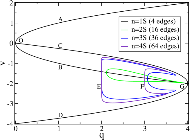
Figure 10: Roots of $P_{B}(q,v)$ for the Potts model on the square lattice, using $n\times n$ square bases. The bases are labelled $n$S in the figure legend (S stands for “square”). The letters appearing in the figure are explained in the main text.

To get a better idea about what to expect for other lattices, we show in Fig. 10 the manifolds $P_{B}(q,v)=0$ for the square-lattice Potts model with $n\times n$ square bases of size $n\leq 4$. The critical polynomials are obtained within the transfer matrix formalism of section 3 by using the building block

$${\sf B}_{i}={\sf H}_{i}{\sf V}_{i}{\sf V}_{i+1}{\sf H}_{i}\,.$$ (48)

The small factors (2), appearing in each of the $P_{B}(q,v)$, produce the selfdual critical curves $v^{2}-q=0$ (denoted A and B) and the dual pair of antiferromagnetic transition curves $v^{2}+4v+q=0$ (denoted C and D). The remaining large factor in $P_{B}(q,v)$, of degree $|E|-4$ in the $v$ variable, produces dual pairs of curves inside the C and D curves, in the form of “bubbles” to the left of the point $(q,v)=(4,-2)$, denoted G. Each bubble intersects the self-dual transition curve $v=-\sqrt{q}$ (denoted B) in two points. The corresponding $q$ values, $q_{\rm c}^{(1)}$ and $q_{\rm c}^{(2)}$, are given in Table 6. It appears that they converge very fast to $B_{4}=2$ and $B_{6}=3$ upon increasing $n$. Figure 10 provides convincing evidence that in the limit $n\to\infty$ each of these two points will be part of a vertical ray (E and F) extending between the antiferromagnetic curves (C and D).

While this is in line with the general expectations outlined above, the possible connexion between $P_{B}(q,v)$ and the studies [34, 35] of partition function zeros remains rather indirect. In particular, it remains an open question at this stage whether yet larger bases might lead to the formation of vertical rays at other Beraha numbers than $B_{4}$ and $B_{6}$.

$n$	$q_{\rm c}^{(1)}$	$q_{\rm c}^{(2)}$
2	2.032 815 790 358 187	4.000 000 000 000 000
3	2.000 010 742 629 917	3.064 263 890 473 626
4	2.000 000 000 040 606	3.000 370 123 813 456
$\infty$	2	3

Table 6: Crossings of the “bubbles” in Figure 10 with the critical curve $v=-\sqrt{q}$.

5.2 $(4,8^{2})$ lattice

In the following three subsections we discuss the lattices which are the subject of this study. We have arranged them in order of increasing complexity of their critical manifolds. We begin with the $(4,8^{2})$ lattice, whose phase diagram turns out to be very similar to that of the square lattice.

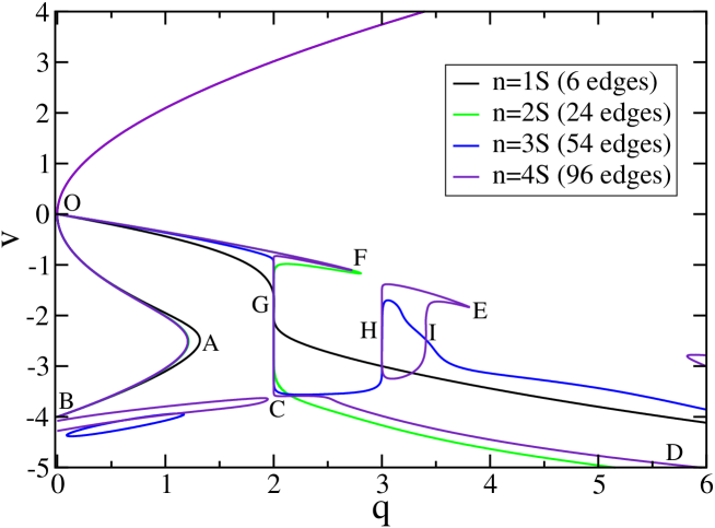
Figure 11: Roots of $P_{B}(q,v)$ for the Potts model on the $(4,8^{2})$ lattice, using $n\times n$ square bases.

The roots of $P_{B}(q,v)$ for square bases of size $n\leq 4$ are shown in Figure 11. In the ferromagnetic region the curves are indistinguishable on the scale of the figure (see section 4 for details). However, the close-up on the antiferromagnetic region, presented in Figure 12, reveals considerable finite-size effects. The question naturally arises which parts of these curves provide reliable information about the critical manifold in the thermodynamical limit.

Obviously, the pieces such as OAB (the letters refer to Figure 12), where all four curves are almost coincident, can be expected to form part of the true critical manifold. In particular we note that all curves go exactly through the point B with coordinates $(q,v)=(0,-4)$. By duality, and using results of [36], we can therefore deduce that spanning forests on the dual (union-jack) lattice undergo a phase transition when the weight of each component tree is $w_{c}=-4$.

Other parts of the curves, such as the stretched-out bubbles extending from B to C, only emerge for sufficiently large $n$ (here, for $n\geq 3$). This is true as well for the vertical rays that build up at G, H and I. In analogy with the square-lattice case, we expect the first two rays (at G and H) to be have $q$ coordinate $B_{4}=2$ and $B_{6}=3$. There is good evidence for conjecturing that the last ray (at I) is situated at $B_{8}=2+\sqrt{2}=3.414\,213\cdots$. The prong advancing at F seems to close up the space between the G and H vertical rays. Similarly, the prong advancing at E makes it plausible that in the $n\to\infty$ limit the “upper curve” OFE will extend to $q=4$, turn around, and join the “lower curve” containing BC.

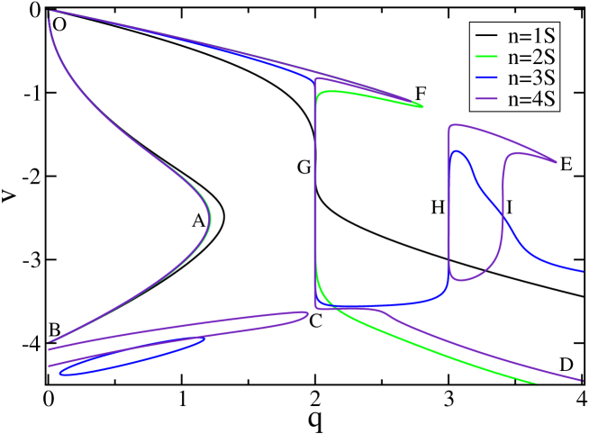
Figure 12: Close-up on the antiferromagnetic region of Figure 11.

From these pieces of information we arrive at the following expectations—or conjectures—for the critical manifold in the continuum limit. The curve OAB and the ferromagnetic critical curve will remain. Other curves will extend to infinity in the antiferromagnetic regime, such as the one marked D in Figure 12, and possibly another emanating from E. The Berker-Kadanoff phase will be bordered by the curve OFEPCB, where P is a point with $q=4$. Inside this phase there will be vertical rays at $q=B_{4},B_{6},B_{8},B_{10},\ldots$ (the figure provides good evidence for the first three rays at letters G, H and I). Moreover, by analogy, we conjecture that the square-lattice model will have the same infinite set of rays (although Figure 10 only provides evidence for the first two of them).

5.3 Kagome lattice

In the case of the kagome lattice we have more information, since $P_{B}(q,v)$ has been computed with both square and hexagonal bases. On the other hand, the phase diagram is more complicated. As already pointed out in [1], no basis—however big—is likely to reveal all aspects of the critical manifold, and the general picture can only be understood by carefully comparing the results from different bases and embeddings.

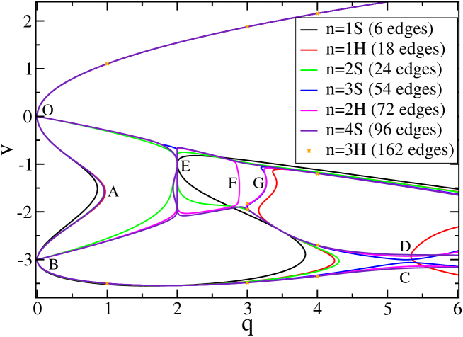
Figure 13: Roots of $P_{B}(q,v)$ for the Potts model on the kagome lattice. In the figure legend, the square bases are labelled $n$S, while $n$H denote the hexagonal bases.

The roots of $P_{B}(q,v)$ are shown in Figure 13. The continuation of the ferromagnetic critical curve goes through OAB, through the point C, and out to infinity. Two other branches go to infinity in the antiferromagnetic region: one labelled D and another emanating from G. Notice that the two branches C and D are not visible with the smaller bases, since the curves join up and turn around at $q\approx 4$.

The antiferromagnetic region contains interesting new features, as shown in the close-up in Figure 14. As before, there are vertical rays developing at $q=B_{4}$ (labelled E) and at $q=B_{6}$ (labelled F). Notice that the latter ray (F) is only revealed by the $n=2$ hexagonal basis; this nicely illustrates the remark made in the first paragraph of this subsection. There also seems to be parity effects in the size $n$ of the square bases. For instance, although the segment near G is present in both hexagonal bases, and in the $n=3$ square basis, it is absent from the larger $n=4$ square basis. The fact that the $n=3$ square and $n=2$ hexagonal curves are almost coincident near G makes it likely that this segment will not move much further upon increasing $n$. In particular, we note that this segment is unlikely to become a vertical ray, and therefore presumably is the rightmost termination of the Berker-Kadanoff phase. If so, there will be only two vertical rays (at $B_{4}$ and $B_{6}$) for this lattice.

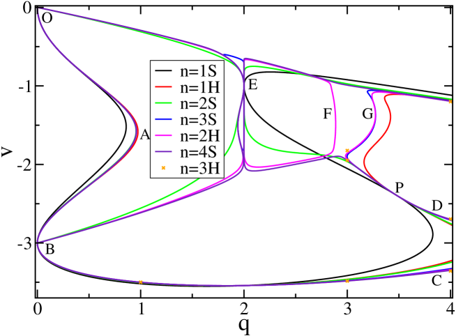
Figure 14: Close-up on the antiferromagnetic region of Figure 13.

The vertical extent of the rays at E and F reveals that the Berker-Kadanoff phase is not bounded from below by BC, but rather by another curve that emerges from B with positive slope.

Further magnification, shown in Figure 15, unearths an interesting detail in the region $q\approx 2$. Indeed, there is an “unexpected curve” emanating from $(q,v)=(2,-1)$, exactly for any $n$, that goes to the left through a point $\approx(1.94,-1.5)$ and ends near $(2,-2)$. On the scale of Figure 13 this produces a very narrow sliver that one would be likely to dismiss as a finite-size effect. But on the scale of Figure 15 it becomes clear that the different bases produce almost coincident results for the location of the unexpected curve. We therefore believe that this unexpected curve is a real effect that will persist in the thermodynamical limit.

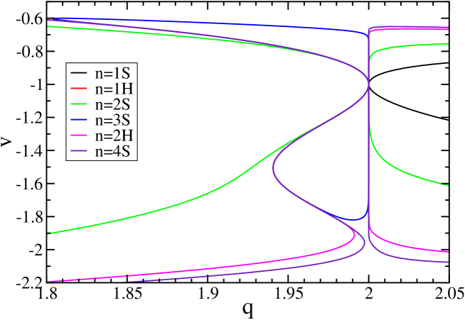
Figure 15: Tiny detail of Figure 13 in the region $q\approx 2$.

We remark that in the thermodynamical limit the critical manifold should contain the point $(q,v)=(3,-1)$ exactly. Indeed, one can show [37] that the three-state zero-temperature antiferromagnet on the kagome lattice is equivalent to the corresponding four-state model on the triangular lattice. The latter is known to be critical with central charge $c=2$ (see [37] and references therein). Our finite bases locate the antiferromagnetic transition in the $q=3$ model at

$$v_{\rm c}^{\rm AF}(q=3)=\left\{\begin{array}[]{lll}-0.921\,400\,117\cdots&\mbox{(6-edge basis)}\\ -0.973\,665\,377\cdots&\mbox{(24-edge basis)}\\ -0.990\,228\,473\cdots&\mbox{(96-edge basis)}\\ \end{array}\right.$$ (49)

and it seems likely that this might indeed tend to $v_{\rm c}^{\rm AF}(q=3)=-1$ in the thermodynamical limit.

Note finally that all curves pass through $(q,v)=(0,-3)$ exactly. Using again [36], this implies that on the dual (diced) lattice, the problem of spanning forests [36] has a critical point with a weight per tree $w_{\rm c}=-3$.

5.3.1 A peculiar critical point

Close inspection of Figure 14 reveals that the curves for any basis—be it square or hexagonal—go through the common point P with coordinates $(q,v)\approx(3.477,-2.393)$. This is strong evidence that P might actually be an exact critical point for the kagome-lattice Potts model. We now show that this is indeed the case, and we determine the coordinates and universality class of P exactly.

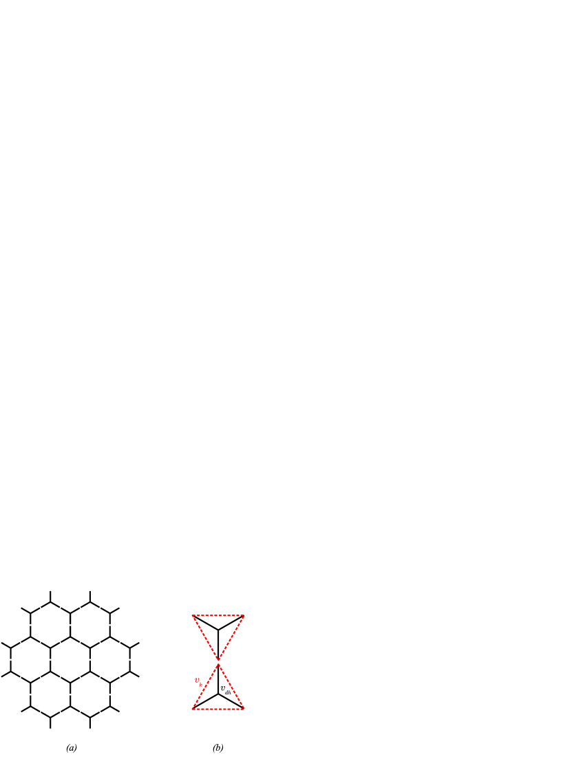
Figure 16: a) The hexagonal lattice with doubled edges; b) a star-triangle replacement that gives the kagome lattice.

The crux of the argument is to relate the kagome lattice to a decorated hexagonal lattice, by means of a star-triangle transformation. This is illustrated in Figure 16. The latter lattice can in turn be transformed into a standard hexagonal lattice, for which the exact critical curve is given by (4).

Let us denote by $K_{\rm k}$ and $K_{\rm dh}$ the couplings between neighbouring Potts spins on the kagome and decorated hexagonal lattice, respectively. Assume initially $q$ integer; the argument eventually carries over to non-integer $q$ by analytical continuation. The star-triangle transformation then reads

$$\sum_{\sigma_{0}=1}^{q}{\rm e}^{K_{\rm dh}(\delta_{\sigma_{1},\sigma_{0}}+\delta_{\sigma_{2},\sigma_{0}}+\delta_{\sigma_{3},\sigma_{0}})}=A{\rm e}^{K_{\rm k}(\delta_{\sigma_{1},\sigma_{2}}+\delta_{\sigma_{2},\sigma_{3}}+\delta_{\sigma_{3},\sigma_{1}})}\,,$$ (50)

where $\sigma_{1},\sigma_{2},\sigma_{3}$ denote the three exterior spins common to a triangle and its inscribed star; $\sigma_{0}$ is the internal spin of the triangle; and $A$ is a proportionality constant to be determined. The relation (50) must hold for any choice of the exterior spins. The three possible cases — 1) $\sigma_{1}=\sigma_{2}=\sigma_{3}$; 2) $\sigma_{1}=\sigma_{2}\neq\sigma_{3}$; and 3) all three spins different — lead to the equations

$${\rm e}^{3K_{\rm dh}}+(q-1) = A{\rm e}^{3K_{\rm k}}\,,$$ (51)

$${\rm e}^{2K_{\rm dh}}+\rm e^{K_{\rm dh}}+(q-2) = A{\rm e}^{K_{\rm k}}\,,$$ (52)

$$3{\rm e}^{K_{\rm dh}}+(q-3) = A\,.$$ (53)

Using (53) to eliminate $A$ from Eqs. (51)–(52), and trading the couplings $K$ for the Fortuin-Kasteleyn variables $v={\rm e}^{K}-1$ as usual, we arrive at

$$(v_{\rm dh}+1)^{3}+q-1 = \big{(}3(v_{\rm dh}+1)+q-3\big{)}(v_{\rm k}+1)^{3}\,,$$ (54)

$$(v_{\rm dh}+1)^{2}+(v_{\rm dh}+1)+q-2 = \big{(}3(v_{\rm dh}+1)+q-3\big{)}(v_{\rm k}+1)\,.$$ (55)

The decorated hexagonal lattice can be transformed into a standard hexagonal lattice by applying the series reduction formula [19] to turn the double edges into simple edges. This reads

$$v_{\rm h}=\frac{v_{\rm dh}^{2}}{q+2v_{\rm dh}}\,.$$ (56)

The resulting hexagonal-lattice Potts model is critical when (4) is satisfied, that is

$$v_{\rm h}^{3}-3qv_{\rm h}-q^{2}=0\,.$$ (57)

There are two real solutions of the equations (54)–(57). The first one reads

$$q=2\,,\qquad v_{\rm k}=-1\,,\qquad v_{\rm h}=v_{\rm dh}=-2\,.$$ (58)

Indeed all the kagome-lattice critical polynomials have a root at $(q,v_{\rm k})=(2,-1)$. But more interestingly, we have the real solution

$$q=3.476\,950\,573\,042\,399\cdots\,,\qquad v_{\rm k}=-2.392\,646\,781\,702\,640\cdots\,,$$ (59)

explaining the point P. Note that this corresponds to $v_{\rm dh}\approx-1.453$ and $v_{\rm h}\approx 3.701$, so the equivalent coupling on the hexagonal lattice is positive. It is well-known from conformal field theory and exact solutions that the ferromagnetic phase transition on any lattice with $q=\big{(}2\cos(\pi e_{0})\big{)}^{2}$ is second order with central charge $c=1-\frac{e_{0}^{2}}{1-e_{0}}$. The universality class of the transition at point P is therefore characterised by

$$c=0.905\,667\,155\,343\,907\cdots\,.$$ (60)

5.4 $(3,12^{2})$ lattice

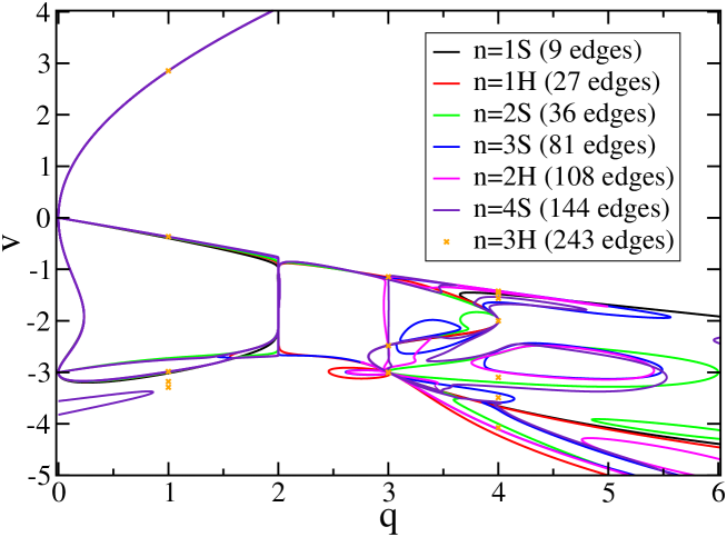
Figure 17: Roots of $P_{B}(q,v)$ for the Potts model on the $(3,12^{2})$ lattice. The square (resp. hexagonal) bases of size $n$ are labelled $n$S (resp. $n$H).

The critical manifold obtained from studying the roots of $P_{B}(q,v)$ on the $(3,12^{2})$ lattice is shown in Figure 17. This is considerably more involved than for the other lattices studied this far. A close-up on the antiferromagnetic region is depicted in Figure 18.

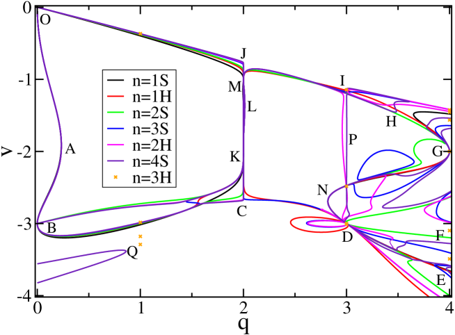
Figure 18: Close-up on the antiferromagnetic region of Figure 17. The various letters are referred to in the main text.

The curve OAB is well-converged as usual. As in the kagome case, there are two curves originating from B, namely BK and BC, but unlike the kagome case both now end on the vertical ray CJ at $q=B_{4}$. Another prong Q, visible only from the largest basis, might eventually provide further curves going towards C, or beyond.

Note that the point B is at $(q,v)=(0,-3)$ exactly, implying [36] that spanning forests on the dual (asanoha, or hemp leaf) lattice have a critical fugacity $w_{c}=-3$ per component tree.

The lower boundary of the Berker-Kadanoff phase, BC, goes on via CD, where it encounters another vertical ray P at $q=B_{6}$, extending between D and I. There are some horizontally elongated “bubbles” near D, but since their size decreases with $n$ it is uncertain whether they persist in the thermodynamical limit. Meanwhile, the upper boundary of the Berker-Kadanoff phase starts out as OJI. The region $3\leq q\leq 4$ is particularly complicated and will be discussed further below.

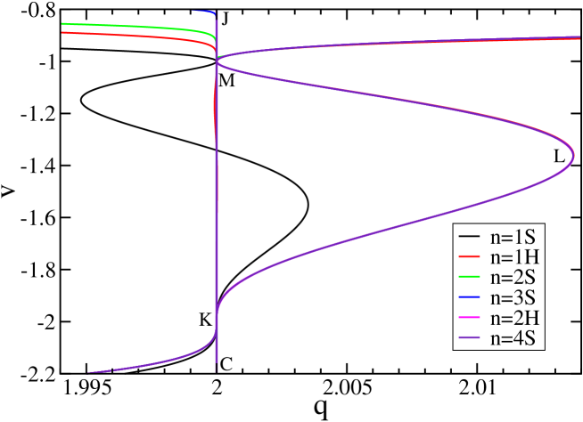
Figure 19: Tiny detail of Figure 17 in the region $q\approx 2$.

Like for the kagome lattice, there are interesting details in the region $q\approx 2$. This is shown in magnification in Figure 19. There is again an “unexpected curve” emanating from point M with coordinates $(q,v)=(2,-1)$, exactly for any $n$, that goes now to the right through point L with $(q,v)\approx(2.014,-1.35)$, for all but the smallest ($n=1$ square) basis, and ends at point K with $(q,v)=(2,-2)$, again exactly for any $n$. Once again, the agreement between the largest bases is such that we can believe that this unexpected curve will subsist in the thermodynamical limit.

The most complicated region is shown enlarged in Figure 20. The boundary of the Berker-Kadanoff phase might be given by DGHI. Note that the point G is $(q,v)=(4,-2)$, exactly for all the biggest sizes. Several of the curves contain “wrinkles” or other signatures close to $q=B_{8}=3.414\,213\cdots$, such as the one labelled H. We take this as a sign of an emergent vertical ray at $B_{8}$. In conjunction with the fact that point G has $q=B_{\infty}=4$, this leads us to believe that the thermodynamical limit will in fact have vertical rays at all $B_{2k}$ with $k\geq 2$.

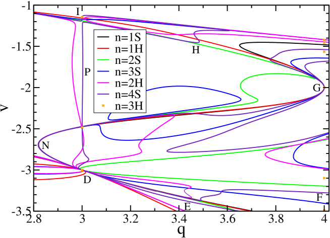
Figure 20: Magnification of the region with $2.8\leq q\leq 4$ in Figure 17.

We further remark that many curves pass through $(q,v)=(3,-3)$ exactly. By duality, this means that the $3$-state Potts antiferromagnet on the dual (asanoha) lattice should undergo a phase transition at zero temperature.

The curve DNG inside the Berker-Kadanoff phase should also be noticed. Finally, there are several curves going from D towards infinity, such as those marked E and F in Figure 18.

6 Discussion

In this work, we have given a new definition of the critical polynomial for the $q$-state Potts model that we had previously defined by the contraction-deletion identity [1]. This has allowed us to compute these polynomials for various lattices using the transfer matrix, a method that permits the use of much larger bases, and therefore the calculation of much higher-degree polynomials, than the contraction-deletion algorithm. Our results put beyond doubt the conjecture that critical polynomials, when they do not provide the exact critical frontier, give excellent approximations that approach the exact answer in the limit of infinite bases. In the ferromagnetic regime, we were able to locate critical couplings on the kagome, $(4,8^{2})$ and $(3,12^{2})$ lattices for $q=3$ and $q=4$ with accuracy rivaling or exceeding that of traditional Monte Carlo or transfer matrix diagonalisation methods. Moreover, the polynomial estimates for $q=3$ are comparable in precision to those for $q=4$, and thus appear not to suffer from the logarithmic corrections to scaling that plague standard numerical techniques for $q=4$.

Critical polynomials also give a clear look at the antiferromagnetic region of the phase diagram, including the Berker-Kadanoff phase, which had previously been difficult to observe numerically. For the square lattice, we find predictions that are completely consistent with theoretical understanding of the BK regime, with vertical rays located at the Beraha numbers $B_{4}$ and $B_{6}$. For the other lattices studied here, on which less is known about the antiferromagnetic region, we find qualitatively similar behaviour, but with notable differences. On the kagome lattice, we observed a previously unknown point in the AF region that the polynomials for every basis placed on the critical curve. Given this information, we were able to find an argument that established this as an exact critical point of the kagome Potts model by a transformation from a decorated hexagonal lattice. This demonstrates the power of the critical polynomial method beyond the numerical determination of critical points — parameters of potential exact solutions are prominently displayed in the phase diagram. It seems likely that there remain many others to be found in this way. Similarly, on the kagome and $(3,12^{2})$ lattices, we have found unexpected critical curves within the Berker-Kadanoff phase that are predicted by a range of bases, indicating that they very likely represent real features of the phase diagrams. The presence of these curves awaits a theoretical explanation.

Several factors determine the accuracy of the predictions made by the critical polynomial method. Generally speaking, the best accuracy is obtained in the ferromagnetic region ($v>0$). On the other hand, we have observed for all lattices studied here that the critical points of the Ising model ($q=2$) come out exactly, even when they are situated in the antiferromagnetic region ($v<0$). A similar phenomenon holds true for $q=0$, insofar as all the curves pass exactly through the origin $(q,v)=(0,0)$ as well as through another point $(0,v)$, with $v=-4$ for the square and $(4,8^{2})$ lattices, and $v=-3$ for the kagome and $(3,12^{2})$ lattices. We have seen that other exact points may appear as well on certain lattices. The limits $q\to\infty$ can also easily be shown to be exact, in the sense that the critical polynomial provides the correct asymptotic behaviour as predicted by first-order phase coexistence in the Fortuin-Kasteleyn expansion [1]. Outside these exact points and limits, the accuracy obviously depends on the size of the basis, and on the compatibility of its embedding with the symmetries of the lattice. For example, hexagonal bases fare better than their square counterparts when the lattice has a 3-fold rotational symmetry. For square bases the twist also seems to play a role, with the untwisted bases being the most accurate for the kagome and $(3,12^{2})$ lattices, and by contrast, the maximally twisted bases performing better for the $(4,8^{2})$ lattice. Finally, as an empirical rule, it appears that the accuracy deteriorates with increasing distance along the curve from one of the exact cases. A good example of that point is the comparatively mediocre precision with which the method accounts for the known $(q,v)=(3,-1)$ critical point of the kagome-lattice Potts model; see (49).

Because this method is relatively new, the ultimate limit on the size of basis that can be employed on each lattice is not yet completely clear. Here, we were able to find polynomials of degree up to 243 using a large parallel calculation. However, improvements are certainly possible and it will hopefully come to be seen as a worthy computational challenge to push this limit even further. Aside from optimising performance, there remains a great deal to be explained about the critical polynomial method. The fact that it works so well at predicting unsolved critical manifolds is still quite mysterious. Although one can argue that universality guarantees equation (13) will give estimates that approach the correct value for infinite $B$, it is surprising how accurate the results are for small bases. It is clear that the condition (13) reveals some larger truth about critical Potts systems, the full mathematical implications of which are yet to be discovered.

References

References

- [1] Jacobsen J L and Scullard C R 2012 arXiv:1204.0622
- [2] Potts R B 1952 Proc. Camb. Phil. Soc. 48 106
- [3] Wu F Y 1982 Rev. Mod. Phys. 54 235
- [4] Baxter R J 1982 Exactly solved models in statistical mechanics (Academic Press, London)
- [5] Fortuin C M and Kasteleyn P W 1972 Physica 57 536
- [6] Baxter R J 1973 J. Phys. C 6 L445
- [7] Baxter R J, Temperley H N V and Ashley S E 1978 Proc. Roy. Soc. London A 358 535
- [8] Wu F Y 2010 Phys. Rev. E 81 061110
- [9] Scullard C R 2006 Phys. Rev. E 73 016107
- [10] Ziff R M 2006 Phys. Rev. E 73 016134
- [11] Wierman J C 1984 J. Phys. A: Math. Gen. 17 1525
- [12] Ding C, Wang Y and Li Y 2012 Phys. Rev. E 86 021125
- [13] Scullard C R and Jacobsen J L 2012 arXiv:1210.7845
- [14] Baxter R J 1982 Proc. Roy. Soc. London A 383 43
- [15] Scullard C R 2012 Phys. Rev. E 86 041131
- [16] Scullard C R 2012 arXiv:1207.3340
- [17] Ziff R M and Suding P N 1997 J. Phys. A: Math. Gen. 30 5351
- [18] Wu F Y 1979 J. Phys. C 12 L645
- [19] Sokal A D 2005 London Math. Soc. Lect. Note Ser. 327 173
- [20] Scullard C R and Jacobsen J L 2012 arXiv:1209.1451
- [21] Wu F Y and Lin K Y 1980 J. Phys. A 13 629–636
- [22] Blöte H W J and Nightingale M P 1982 Physica A 112 701
- [23] Jacobsen J L and Cardy J 1998 Nucl. Phys. B 515 701
- [24] Salas J and Sokal A D 2001 J. Stat. Phys. 104 609
- [25] Baxter R J, Kelland S B and Wu F Y 1976 J. Phys. A: Math. Gen. 9 397
- [26] Kano K and Naya S 1953 Prog. Theor. Phys. 10 158
- [27] Ding C, Fu Z, Guo W and Wu F Y 2010 Phys. Rev. E 81 061111
- [28] Hurst C A 1963 J. Chem. Phys. 38 2558
- [29] Syozi I 1955 Rev. Kobe Univ. Mercantile Marine 2 21
- [30] Saleur H 1991 Nucl. Phys. B 360 219
- [31] Jacobsen J L and Saleur H 2006 Nucl. Phys. B 743 207
- [32] Pasquier V and Saleur H 1990 Nucl. Phys. B 330 523
- [33] Andrews G E, Baxter R J and Forrester P J 1984 J. Stat. Phys 35 193
- [34] Jacobsen J L and Salas J 2006 J. Stat. Phys. 122 705
- [35] Jacobsen J L and Salas J 2007 Nucl. Phys. B 783 238
- [36] Jacobsen J L, Salas J and Sokal A 2005 J. Stat. Phys. 119 1153
- [37] Moore C and Newman M E J 2000 J. Stat. Phys. 99 629