Helicity Condensation as the Origin of Coronal and Solar Wind Structure

Abstract

Three of the most important and most puzzling features of the Sun’s atmosphere are the smoothness of the closed field corona, the accumulation of magnetic shear at photospheric polarity inversion lines (PIL), and the complexity of the slow wind. We propose that a single process, helicity condensation, is the physical mechanism giving rise to all three features. A simplified model is presented for how helicity is injected and transported in the closed corona by magnetic reconnection. With this model we demonstrate that helicity must condense onto PILs and coronal hole boundaries, and estimate the rate of helicity accumulation at PILs and the loss to the wind. Our results can account for many of the observed properties of the closed corona and wind.

1 Introduction

A classic, but puzzling feature of the Sun’s high-temperature ($>1$MK) atmosphere is its apparent lack of complexity. High-resolution XUV and X-ray images of the closed-field corona, such as those from the Transition Region and Coronal Explorer (TRACE) mission, invariably show a smooth collection of loops (e.g. Schrijver et al., 1999). If the underlying photospheric flux distribution is highly structured with several polarity regions, then the topology of the loops in the corona will appear complex in XUV images, but this is only due to seeing through multiple flux systems. The surprising result is that the loops in any one flux system, such as a bipolar active region, are generally not observed to be twisted or tangled. Since the coronal field is line-tied to the photosphere, which is undergoing continuous chaotic motions due to the convective flows, it would seem that geometrical complexity should eventually appear in the coronal field. Instead, the magnetic field appears to remain laminar and not far from a potential state over most of the corona. Extrapolations of the field do indicate the presence of coronal currents (Leka et al., 1996; Tian et al., 2005), but these are large-scale volumetric currents that produce only a global shear or twist rather than field line tangling (Schrijver, 2007).

The observation that loops are untangled, at least on present observable scales, is especially surprising given that the corona is being heated continuously. The standard theory for the heating is that the energy is due to stressing of the coronal field by the random motions of the photospheric footpoints. This is the basic idea of Parker’s nanoflare model and similar theories (Parker, 1972, 1983, 1988; van Ballegooijen, 1986; Mikic et al., 1989; Berger, 1991; Rappazzo et al., 2008). The photospheric motions are postulated to tangle and braid the field lines, producing small scale current sheets, which then release their energy via reconnection. A great deal of work has been done applying this nanoflare scenario to coronal observations with considerable success (Klimchuk, 2006).

The problem with such reconnection-heating models is that any helicity injected into the corona as a result of the motions is expected to survive, because reconnection in a high Lundquist-number system like the corona conserves magnetic helicity (Taylor, 1974; Berger, 1984). Consequently, even if it is injected on scales below present-day resolution, $<1$ arcsecond, the helicity should build up and appear as twisting or tangling of the large-scale coronal field. Note also that even if the degree of tangling required for the heating is small – for example, Parker estimates a misalignment angle between the reconnecting stressed field and the initial potential state of only $20^{\circ}$ or so (Parker, 1983) – any net helicity injected by the stressing should continue to accumulate and eventually produce large-scale observable effects. We conclude, therefore, that both the basic observations of photospheric motions and the reconnection theories for coronal heating imply that the coronal field should have a complex geometry, in direct disagreement with observations.

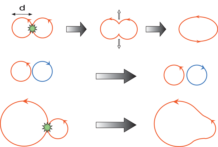
Figure 2: Interaction of the twist component of interacting flux tube. Red and blue circles correspond to oppositely-oriented twist components of the magnetic field.

There are, at least, two seemingly likely explanations for this disagreement. The first is that photospheric motions produce equal and opposite helicity everywhere, so that no net helicity is injected into the corona. Nanoflare reconnection then simply cancels out the positive and negative helicities. This explanation, however, has both observational and theoretical difficulties. Numerous observations imply that photospheric motions, including flux emergence, do inject a net helicity into each hemisphere. For example, observations of prominence structure (Martin et al., 1992; Rust, 1994; Zirker et al., 1997; Pevtsov et al., 2003) and of active region vector fields (Seehafer, 1990; Pevtsov et al., 1995) indicate a strongly preferred sign for the helicity injected into each solar hemisphere, possibly related to the differential rotation (DeVore, 2000). Furthermore, theory and numerical simulations (Linton et al., 2001) have shown that, for magnetic flux tubes with parallel axial fields, reconnection occurs only if the tubes have the same sign of helicity, the so-called co-helicity case as discussed by Yamada et al. (1990). Flux tubes with opposite helicity only bounce when they collide (Linton et al., 2001); therefore, reconnection cannot cancel out positive and negative injected helicity in interacting coronal loops. This point will be clarified in Figure 2 below.

The other possible explanation for the lack of helicity buildup is that the heating is due not to reconnection, but to true diffusion, in which case helicity is not conserved. This hypothesis was proposed by Schrijver (2007) to explain the TRACE images. He argued that continual reconnection induced by the rapidly varying field of the magnetic carpet (Harvey, 1985; Schrijver et al., 1997) causes the chromosphere and transition region to act like a high-resistivity layer. Coronal loop field lines can slip along this layer and, thereby, lose their tangles. This explanation, however, also has theoretical and observational difficulties. Reconnection is not physically equivalent to diffusion, no matter how frequent the reconnection. Diffusion does destroy helicity and will relax a magnetic field back down to its minimum energy potential state, but reconnection can relax the system down only to some state compatible with total helicity conservation, such as a linear force-free state (Taylor, 1974, 1986). In fact, for the line-tied corona, we have argued that helicity imposes very stringent constraints on the possible end state of a system undergoing reconnection relaxation (Antiochos et al., 2002).

Furthermore, observations imply that whenever helicity is, indeed, present in the corona, it does not show evidence for diffusive decay. The largest concentration of coronal helicity is in filaments and prominences, or more precisely, in the strongly sheared field that defines a filament channel (e.g. Tandberg-Hanssen, 1995; Mackay et al., 2010). Although there is still debate over the exact topology of the filament channel magnetic field; in particular, whether it is a sheared arcade (Antiochos et al,, 1994) or a twisted flux rope, the models agree that for a physically realistic 3D topology all the filament flux must be connected to the photosphere. Consequently, if the chromosphere or transition region really did contain a high-resistivity layer, the filament channel shear would simply disappear by field-line slippage. Such slippage is never observed; if anything, filament shear seems to increase continuously until it is ejected from the corona with a filament eruption/CME.

From the discussion above, we conclude that a net helicity is injected into each coronal hemisphere by the photosphere, and that reconnection preserves this helicity. But, in that case, where does the helicity go? In a sense, the answer is obvious: The helicity injected into the closed-field corona must end up as the magnetic shear in filament channels. These are the only locations in the corona where the magnetic field is strongly non-potential and, hence, has a strong helicity concentration.

Although this answer is intuitively appealing, it seems extremely unlikely. It naturally raises the long-standing questions: What exactly are filament channels and how do they form? Along with laminar coronal loops, filament channels are also classic but puzzling features of the Sun’s atmosphere. These structures consist of low-lying magnetic flux centered about photospheric polarity inversion lines (PIL), in which the chromospheric and coronal magnetic field lines run almost parallel to the inversion line rather than perpendicular, as expected for a potential field (Rust, 1967; Leroy et al., 1983; Martin, 1998). Direct measurements of the filament vector field both in the photosphere (Kuckein et al., 2012) and corona (Casini et al., 2003) show that the component parallel to the PIL is dominant. The channels have narrow widths, of order 10 Mm, but their lengths can be greater than a solar diameter for PILs that encircle the Sun. Filament channels are very common, invariably appearing about any long-lived PIL, both in active regions and quiet Sun. It should be emphasized that the channels are much more common than observable filaments and prominences, which require the presence of substantial amounts of cold plasma as well as the magnetic shear.

Two general mechanisms have been proposed for filament channel formation. One mechanism is flux emergence, specifically the emergence of a sub-photospheric twisted flux rope. Most simulations of flux rope emergence find that the resulting structure in the corona is a sheared arcade localized near the PIL (e.g. Mancester, 2001; Fan, 2001; Magara & Longcope, 2003; Archontis, 2004; Leake et al., 2010; Fang et al., 2012). The basic process is straightforward; the twist component of the sub-photospheric flux rope emerges to become the overlying quasi-potential arcade in the corona, while the axial sub-surface component emerges to become the shear field of the filament channel. It is interesting to note that, in general, the resulting filament channel in the corona is not a twisted flux rope, but a sheared arcade, because the concave-up portion of the flux-rope field lines stays trapped below the surface even in 3D (Fang et al., 2012).

Although flux emergence can yield a sheared arcade, there are major theoretical and observational difficulties with this process as the general mechanism for filament channel formation. First, the simulations have yet to show that flux emergence agrees quantitatively with the amount of flux and degree of shear measured in observed filament channels. In fact, Leake et al. (2010) argue that only a small amount of axial flux emerges, at least in 2.5D simulations, far too small to account for the magnetic free energy in observed filament channels. Similar conclusions have been reached from recent 3D simulations, as well (Fang et al., 2012). A much greater problem for the model is that filament channels are frequently observed to form in regions where there is no apparent flux emergence, such as at PILs between decaying regions and high latitude PILs (e.g. Mackay et al., 2010). Moreover, the emergence of a simple bipolar active region rarely produces a filament channel at its PIL. The channel usually forms only well after the end of the flux emergence, when the active region has decayed and dispersed to interact with surrounding flux regions. Consequently, flux emergence cannot be the only mechanism for filament channel formation.

The second, and perhaps, the most popular mechanism that has been proposed for filament channel formation is flux cancellation (Martin, 1998). The basic picture is that large-scale shear due to differential rotation or flux emergence concentrates at PILs as opposite-polarity photospheric flux converges and cancels there. Note that this mechanism inherently requires reconnection at the photospheric PIL in order to form low-lying loops that can sink and disappear and concave-up loops that can rise into the corona (van Ballegooijen & Martens, 1989). A fundamental difficulty with such reconnection, however, is that it produces a twisted flux rope in the corona just like flare reconnection produces the highly twisted flux rope of a CME. On the other hand, high resolution observations of filaments both from the ground (Lin et al., 2005) and space (Vourlidas et al., 2010) show a field geometry consisting of long, parallel strands, with no evidence of twist or tangling. In fact, empirical models for filaments derived solely from observations, have a laminar field geometry exactly like that of the TRACE loops, except that the field lines are stretched out and primarily horizontal rather than arched (Martin ref). It has been suggested that the large twist component resulting from reconnection may diffuse away (van Ballegooijen, 2004), but as argued above, any diffusion would also decrease the shear component, contrary to observations. Note also that the twist produced by flare reconnection, which is physically identical to flux cancellation reconnection, is never observed to diffuse away, but is measured to persist out to 1 AU (Kumar & Rust, 1996; Qiu et al., 2007).

In addition to the lack of observed twist, the prevalence of filament channels poses severe difficulties for the flux cancellation model and, indeed, for any model. As stated above, filament channels are ubiquitous, appearing over all types of PILs ranging from the most complex and strongest active regions to very quiet high-latitude regions. In fact, it is not uncommon to observe a filament channel that continues unbroken over a PIL that passes from an active region into neighboring quiet region with the cold material, itself, transitioning smoothly from a typical low-lying active region filament to a high-lying quiet sun filament (e.g. Su & van Ballegooijen, 2012). Given these observations, it seems improbable that filament channels are due to some phenomenon in the plasma-dominated photosphere, because the dynamics there are insensitive to the magnetic field structure and, in particular, to whether a PIL is present or not. This is especially true in the weak-field regions where quiescent prominences typically form (Klimchuk, 1987). It seems much more likely that filament channel formation is due to some generic process occurring in the magnetically-dominated corona and upper chromosphere.

We propose that the origin of filament channels is the reconnection-driven evolution of helicity injected into the closed-field corona. This hypothesis seems counterintuitive, because coronal-loop helicity is injected on small scales more-or-less uniformly throughout the corona, whereas filament channels are coherent structures, localized only around PILs and extending to very large scale. In this paper, we describe a process, helicity condensation, that performs exactly the required transformation of small-scale coronal loop helicity into large-scale filament-channel shear. Helicity condensation keeps coronal loops laminar while shearing filament channels.

Furthermore, helicity condensation may be responsible for much of the complex structure and dynamics observed in the slow solar wind. We argued above that the helicity injected into the corona must end up in filament channels, but in regions containing coronal holes, another possibility is that some helicity is ejected out into the wind by the opening of closed flux at the coronal hole boundary. Such helicity transfer is implicitly present in the S-Web model for the slow wind (Antiochos et al., 2011, 2012), which postulates that this wind is due to continual dynamics of the open-closed flux boundary. If so, then helicity condensation also will play a major role in the origin and properties of the slow solar wind.

We describe below the basic process of helicity condensation and derive estimates of its effectiveness in the Sun’s corona.

2 A Model for Helicity Injection and Transport

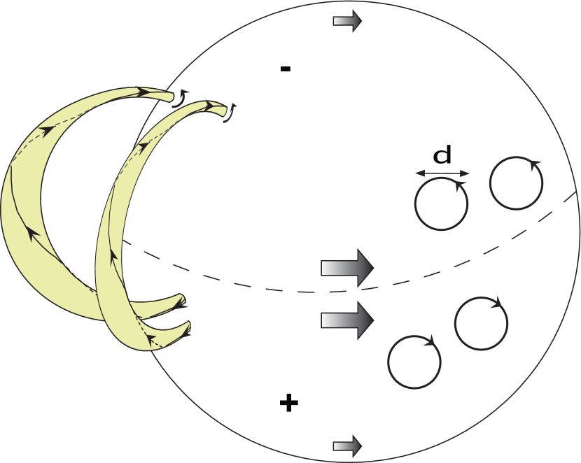
Figure 1: Model for helicity injection into the corona by photospheric motions. The primary effect of the motions is to inject an effective twist of scale d. The sense of the twist in each hemisphere is determined by the differential rotation, large arrows. The yellow arches represent two neighboring coronal loops (magnetic flux tubes).

In order to understand how magnetic helicity is likely to evolve in the corona, we must first consider the injection process. Assume, for the moment, that the photospheric flux distribution consists of only two polarity regions as shown in Figure 1: a negative northern hemisphere and a positive south, so that all the flux closes across the equatorial PIL (dashed line). The yellow arches in the figure denote two arbitrary small flux tubes corresponding to coronal loops or to the strands inside an observable coronal loop. The quasi-random photospheric motions will introduce small-scale structure and inject helicity to this coronal field. Helicity will also be injected by large-scale motions, such as differential rotation, and by flux emergence/cancellation, such as the magnetic carpet, but for simplicity let us model the injection as due to the continual small-scale photospheric motions, in particular, the granular or supergranular flows. Note that if the magnetic carpet dynamics do not change the net coronal flux, their effect on the coronal helicity can be captured by effective photospheric motions. Furthermore, recent analysis of high-resolution Solar Dynamics Observatory (SDO) data indicates that the bulk of the helicity injected into active regions is due to photospheric motions rather than flux emergence (Liu & Schuck, 2012).

Following the arguments of Sturrock & Uchida (1981), the energy and, certainly, the helicity injected into coronal loops by stochastic horizontal flows at the photosphere will be primarily in the form of twist. Therefore, we model the motions as a set of randomly located and randomly occurring rotations that have fixed spatial and temporal scales. The true photospheric motions are more complex than a set of fixed-scale rotations, but we are interested only in that part of the flow that injects helicity to the corona. Note also that there is some evidence for exactly the pattern of photospheric rotations of Fig. 1 in measurements of the vorticity of the supergranulation (Duvall & Gizon, 2000; Gizon & Duvall, 2003; Komm et al., 2007).

It has been known since the time of Hale (1927) that sunspot whirls have a clear hemispheric preference, counterclockwise in the north and clockwise in the south (Pevtsov et al., 1995), indicating a preferred sense for the helicity of the subsurface solar motions. The same helicity preference, negative in the north and positive in the south, has been well documented to occur in all types of coronal magnetic structures ranging from quiet Sun field to active region complexes (Pevtsov & Balasubramaniam, 2003) and has been observed out in the heliospheric magnetic field (Bieber et al., 1987). As shown in Figure 1, this hemispheric “rule” is in the same sense as would be expected from the surface differential rotation, but the actual mechanism is still not clear. In any case, we expect there to be a preferred sense to the helicity injecting rotations as illustrated in Figure 1. Note that this is only a preference; a fraction of the rotation in each hemisphere could well have the “unpreferred” sense.

The motions shown in Figure 1 have a number of interesting implications for the coronal field. Assuming, for simplicity, that the rotations are solid body, have size $d$, and have magnitude, $\Theta$, then each rotation of a photospheric flux tube with axial flux,

$$\Phi_{d}=\pi d^{2}B_{p}/4,$$ (1)

produces in the corona a twist flux,

$$\Phi_{t}=\Theta\Phi_{d}/\pi,$$ (2)

where $B_{p}$ is the average normal field at the photosphere. In open field regions (not shown in the Figure), this twist flux simply propagates outward, resulting in a net helicity to the turbulence in the fast wind (e.g. Leamon et al, 1998). We will discuss the implications for the slow wind below. In the closed field regions, however, the coronal loops acquire a twist component to their magnetic field, as shown in the Figure. If the loop is perfectly symmetric about the equator, then on average, the twists imposed by the two footpoints cancel out so that no net helicity is injected. Basically, the loop is twisted at one end, but untwisted at the other. On the other hand, if the loop has both footpoints in one hemisphere, as is usually the case when the PIL is not exactly at the equator, then the twist from each footpoint will add. Even if the loop is transequatorial, we do not expect any symmetry for a real coronal loop, so a net twist will still be produced by the footpoint motions. Note also, that the effect of any unpreferred-sense rotations (clockwise in the north and counterclockwise in the south) is only to decrease the rate of twisting. To first order, the unpreferred rotations simply untwist the loops, but it should be emphasized that since the rotations are time varying, they can create higher order topological structure in the field even if the net injected helicity vanishes. All higher order topological features, however, such as the braiding of three flux tubes, are not conserved by reconnection (e.g. Pontin et al., 2011) and are not expected to build up in the corona.

Consider now the interaction of the two twisted flux tubes of Fig. 1 due to some random motion that causes them to collide. In fact, the twist itself will cause the flux tubes to expand and interact. Since their main axial fields are parallel, only the twist components of the flux tubes can reconnect. If the tubes have the same sense of twist (helicity), then at the contact point between the tubes, their twist components will be oppositely directed and, hence, will reconnect. This is illustrated in the three sequences of Fig. 2, where the red and blue circles correspond to field lines of the twist magnetic component. In the top sequence the twist components are in the same sense, so they are oppositely directed at their contact point; consequently, they will reconnect there. Another way of understanding this result is to note that for interacting tubes with the same helicity, the photospheric rotations have a stagnation point between them. It is well known that such stagnation point flows lead to exponentially growing separation of magnetic footpoints and, hence, to exponentially growing currents in the corona (e.g. Antiochos & Dahlburg, 1997), which can drive efficient reconnection. The effect of this reconnection is to spread the twist component over the flux of the two tubes, in other words, the two tubes merge into one globally twisted tube as illustrated in the Figure and as found in simulations of flux-tube collisions (Linton et al., 2001).

On the other hand, if the tubes have opposite twist (helicity), then at their point of interaction the twist components are parallel. As illustrated in the second sequence of Figure 2, there is no reconnection in this case. The tubes simply “bounce” (Linton et al., 2001). This result emphasizes the point made in Antiochos & Dahlburg (1997) that reconnection in the solar corona is highly constrained by line-tying. As a result, the coronal magnetic field cannot simply relax to a minimum energy Taylor (1974) state, which for the opposite twist case corresponds to the initial potential field.

The third sequence in Figure 2 illustrates the effect of continued interaction of same-helicity flux tubes. If a larger-scale merged flux tube reconnects with another tube, the result is further merging of the flux and the spread of the twist to even larger scale. This reflects the well-known result from turbulence studies that magnetic helicity tends to cascade upward in scale (e.g. Biskamp, 1993). A key point is that the scale referred to in our cascade process is the amount of axial flux, which is closely related to, but not identical to the spatial scale. As argued directly below, the helicity cascades up to the largest possible flux scale, which corresponds to all the axial flux inside a single polarity region.

Let us consider the end result of this reconnection-driven helicity cascade. Assume a flux system, as in Figure 3, with simple topology given by a PIL (heavy dashed curve in the Figure) and a separatrix curve somewhere on the photosphere (light dashed curve) that defines all the flux that closes across the PIL. There must be additional PILs on the photosphere, but these are not shown. If the separatrix curve lies in the north, then the flux system is entirely in the north and the twist injected by the photosphere will be predominately counter-clockwise. Since only the relative footpoint motions are significant, we can assume without loss of generality that all the twist is imparted inside the PIL as shown in the Figure.

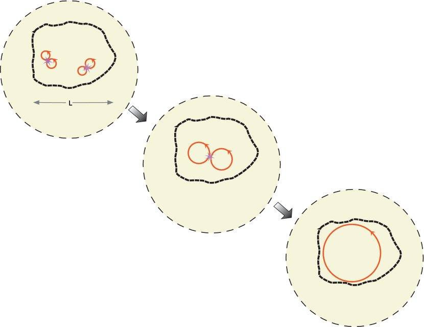
Figure 4: The polarity region of the previous figure as viewed from the north pole.

The expected evolution of this twist is seen in Figure 4, which shows a top view of the flux system. As a result of reconnection, the helicity “condenses” onto the largest scale in the flux system, the PIL, since this encompasses all the flux in the system. The PIL defines the boundary of the polarity region. We conclude, therefore, that the net effect of the many small-scale photospheric twists and the coronal reconnection is to impart a coherent, global twist of the whole flux system that concentrates at the PIL. This global twist is not a true physical motion; the large-scale flux system does not actually rotate as a coherent body, but the photospheric helicity injection and subsequent transport by reconnection does result in an effective global rotation of the magnetic field.

The key point is that such a rotation of the whole flux system corresponds to a coherent localized shear all along the PIL, exactly what is needed to explain the formation of filament channels. Such an effective motion produces a channel consisting of field lines that are sheared but smooth and laminar, with no twist or tangles in agreement with high-resolution observations of prominence threads (Lin et al., 2005; Vourlidas et al., 2010). The coronal reconnection in our helicity condensation model results in a structure that is the direct opposite to that of flux cancellation reconnection, which invariably produces a highly twisted flux rope at the PIL.

Another important point is that the helicity condensation mechanism is unaffected by the shape of the PIL, in particular whether the PIL contains so-called switchbacks where it forms a sharp zigzag. As long as the flux system defined by the PIL is primarily in one hemisphere, helicity condensation will form a filament channel with the same chirality all along that PIL and with roughly the same amount of shear. This result is in contrast to the predictions of some of the flux cancellation models (van Ballegooijen et al., 1998), but is in good agreement with observations (Pevtsov et al., 2003). Furthermore, since the photospheric convection in either quiet or active regions is not observed to change significantly with phase of the solar cycle, the model predicts that the hemispheric helicity rule should hold independent of solar cycle. Again, this conclusion appears to be in good agreement with observations (Pevtsov et al., 2003), unlike some flux cancellation models (Mackay & van Ballegooijen, 2001).

2.1 Rate of Helicity Cascade

Prominences typically form on time scales of several days, which sets a constraint that any model must satisfy; therefore, we calculate below the rate of filament channel formation predicted by the helicity condensation model. Let us consider a polarity region as in Figure 4 with scale $L$ that is large compared to the helicity injection scale $d$. The rate of helicity injection $\eta$ into a flux tube $\Phi_{d}$ by a photospheric twist of average angular velocity $V_{d}/d$ is given by the product of the rate of change of the twist flux of Eq. (2) and the axial flux $\Phi_{d}$, (which stays constant):

$$\eta\approx\Phi_{d}(V_{d}/d)\Phi_{d}$$ (3)

(e.g. Berger, 2000). The total helicity injection rate at the scale $d$ over the whole flux system region with scale $L$ is therefore given by:

$$h_{d}=\Phi_{d}^{2}(V_{d}/d)(L/d)^{2}=(\Phi_{L}/L)^{2}d^{2}\,V_{d}/d,$$ (4)

where $\Phi_{L}$ is the flux of the whole system. Following Kolmogorov’s classic theory for hydrodynamic turbulence (Kolmogorov, 1941), we assume a constant helicity transfer rate at any scale $\lambda$. Therefore:

$$h_{\lambda}=(\Phi_{L}/L)^{2}\lambda^{2}V_{\lambda}/\lambda=h_{d},$$ (5)

which implies that:

$$V_{\lambda}=V_{d}(d/\lambda)\ {\rm and,thus},\ V_{L}=V_{d}(d/L).$$ (6)

It should be noted that unlike $V_{d}$, which is the actual velocity of the photospheric flows, the quantity $V_{L}$ does not represent a true plasma velocity. It is only an effective velocity for the transfer of twist to the largest scale by coronal reconnection. The physical plasma velocities will likely be dominated by reconnection jets and will have both larger magnitude and smaller scale than $V_{L}$. The physical velocities and kinetic energy are expected to cascade downward, not upward, in scale. Consequently, the velocity spectrum $V_{\lambda}$ derived in Eq. 6 may not be directly observable, but the effective velocity $V_{L}$ is indeed physically significant. It quantifies the rate at which magnetic helicity “condenses” out of the corona at the largest scale of the flux system and, hence, $V_{L}$ corresponds to the effective shear velocity along the PIL.

Note also, that the helicity cascade process derived above is somewhat different than the usual hydrodynamic turbulence in which velocity is injected statistically uniformly at some scale and then cascades down to where it is dissipated, usually at a kinetic scale. In such an energy cascade, the injection of kinetic energy at a global scale results in the slow increase of thermal energy (temperature) approximately uniformly throughout the system. In our cascade, however, helicity is injected statistically uniformly at some intermediate scale and then simply piles up at the largest global scale. Even though the helicity injection (i.e., photospheric motions) are uniform, the cascade produces a localized spatial structure in the corona. Helicity condensation in the Sun’s atmosphere is a striking example of self-organization in a complex system.

The time scale for filament channel formation can now be calculated directly from Eq. (6). We note that for the photospheric helicity injection the important parameter is the product of the velocity and the coherence scale of that velocity. Granules typically have $V_{d}\sim 1$ km/s and $d\sim 700$ km, while supergranules have: $V_{d}\sim.25$ km/sec and $d\sim 30,000$ km. Eq. (6) implies that the product $V_{d}\,d$ is the important quantity; therefore, supergranules are expected to dominate the helicity injection. Taking the whole flux system to have scale $d/L\sim 10-100$ implies that a shear of order 1,000 – 10,000 km will build up in $\sim 10^{5}$ s, where we assume that equal helicity is injected at both ends of a flux tube. These results indicate that a high-latitude filament channel with typical shear scales of 100,000 km will form in several days or so, which is consistent with observations (Tandberg-Hanssen, 1995; Mackay et al., 2010). Note also that we expect that the width of the helicity condensation region to be of order the width of the elemental photospheric rotation, $\sim 15,000$ km for supergranules, which again is consistent with the observed widths of filaments (Tandberg-Hanssen, 1995; Mackay et al., 2010).

The supergranular rate of helicity injection estimated above is also consistent with estimates of solar helicity loss to the wind. Taking the system size $L$ to be of order the solar radius $\sim 10^{11}$ cm, and the average field strength at the photosphere to be $~{}\sim 10$ G, we derive from Eq. (4) and the numbers above, a helicity injection rate over the solar surface of $\sim 10^{38}$ Mx/s. Over the course of a full solar cycle, this yields a total helicity loss of $\sim 3\times 10^{46}$ Mx, which agrees well with the inferred losses from observations of CMEs and the wind (DeVore, 2000).

2.2 Implications of the Model

We conclude from the derivation above that helicity condensation can account for filament channel formation, at least, in regions that do not exhibit strong flux emergence. The mechanism can also account for the observed smoothness of coronal loops. Let $\tau$ be the time scale required for the system to establish a steady state (except, of course, at the largest scale $L$ where no steady-state is possible). We expect that $\tau$ is determined by the twist required to produce intense current sheets, of order a full rotation or so (Antiochos, 1998), and not by the rate of reconnection. The driving velocity is only $\sim$ 0.1% of the coronal Alfven speed, so that the reconnection need not be fast in order to keep pace with the driving. For a given $\tau$, the twist angle produced by the effective velocities of Eq. (6) scales as:

$$\Theta_{\lambda}=\tau V_{\lambda}/\lambda\sim\lambda^{-2}$$ (7)

This result implies that the corona will exhibit the most structure at the scale at which the twist is injected (presumably the supergranular scale), and at the largest scale where the helicity piles up, the whole length of the PIL. The so-called coronal cells recently discovered by Sheeley & Warren (2012) appear to be evidence for just this type of structure separation. These authors observe that the large-scale corona breaks up into three distinct structures: flux tubes twisted on a scale of 30,000 km or so, long filment channels along PILs that typically span the whole Sun, and coronal holes. Our helicity condensation model is in excellent agreement with these observations.

An important issue that is raised by the observations and that we have yet to discuss is the effect on the model of a coronal hole or, more generally, of an open field region. Note, also, that even if no coronal hole is present, the simple picture of Figs. 3 and 4 is topologically incomplete. The PIL cannot be the only boundary that defines the closed negative polarity region. At the very least, there must be a point somewhere in the region where a magnetic spine line connects up to a null point Lau & Finn (1990); Antiochos (1990); Priest & Titov (1996); thereby, making this field line effectively open. Of course, real solar polarity regions tend to have much more complexity often containing intricate open field areas and corridors (Antiochos et al., 2011).

Assume that the polarity region of Figs. 3 contains a coronal hole, as illustrated in Figure 5. The presence of the coronal hole introduces subtleties to the calculation of helicity evolution, because the helicity of a truly open field that extends to infinity is not physically meaningful. An open field can have arbitrary helicity due to linkages at infinity where the field vanishes, but the topology does not. Therefore, let us consider instead a system where all the field lines remain closed so the helicity is well-defined throughout the evolution, and let us model the coronal hole as a region where no photospheric twists are imposed; hence, no helicity is injected into this region. In an actual coronal hole twist is injected by photospheric motions, exactly as in closed field regions, but the twist propagates away at the Alfven speed and presumably has no effect on the subsequent evolution in the low corona. Consequently, we can simply model this region as being untwisted.

The analysis of the helicity cascade in the large annular flux region bounded by the PIL and the coronal hole boundary proceeds exactly as above. The only difference is that the total twisted area $L^{2}$ is replaced by $L^{2}-H^{2}$ where $H$ is the scale of the coronal hole. Therefore, the largest scale for the helicity is given by:

$$L^{\prime}=\sqrt{L^{2}-H^{2}}$$ (8)

and the effective velocity for helicity condensation is given by Eq (6) above except that $L$ is replaced by $L^{\prime}$. Also, the twist spectrum, Eq (7) is unchanged. As long as $H<<L$, the presence of the coronal hole has minimal effect on the filament channel formation process, and on the smoothness of coronal loops.

It is evident from Fig. 5, however, that helicity condensation does have an effect on the magnetic field near the coronal hole boundary. We note that twist, or more accurately magnetic shear, also condenses at this boundary, but curiously enough the shear has the sense opposite to that at the PIL. This result may seem physically unlikely, but in fact it is mandated by helicity conservation. The key point is that the shear flux $\Phi_{1}$ that condenses onto the PIL encircles all the photospheric flux in the polarity region, including that in the coronal hole region (“CH”). Therefore, the helicity $H_{1}$ due to this shear flux is given by:

$$H_{1}=\Phi_{1}\Phi_{L^{\prime}}+\Phi_{1}\Phi_{CH},$$ (9)

where $\Phi_{L^{\prime}}$ is the amount of closed photospheric flux inside the PIL and $\Phi_{CH}$ is the amount of photospheric flux in the coronal hole, which can be arbitrary compared to $\Phi_{L^{\prime}}$. But the CH flux is not twisted and never contributes to the helicity injection; hence, it should not affect the helicity condensation at the PIL. The only way to ensure that the CH flux has no effect is to have a shear flux $\Phi_{2}$ that condense at the CH boundary and is exactly equal and oppositely directed to that at the PIL. Such a shear flux encircles only the CH flux and, thereby, adds a helicity contribution:

$$H_{2}=-\Phi_{1}\Phi_{CH},$$ (10)

which exactly cancels out that between the PIL shear flux and the CH. Fig. 5 shows that reconnection would produce just this required shear flux at the CH boundary. In other words, helicity condensation predicts that a filament channel should form at coronal hole boundaries, at the same rate as at the PIL but with the opposite handedness.

These results clearly have major implications for observations. At PILs, the magnetic shear builds up until eventually, it is ejected as a prominence eruption/CME. We expect that a similar process of buildup and ejection occurs at the CH boundaries, but with much less explosive dynamics. The closed field lines near the CH boundary consist of very long, high-lying loops that form the outer shell of the streamer belt. Consequently, it requires far less shear and free energy to open up these loops than to eject the filament channel. We expect that helicity condensation at CH boundaries results in continual small bursts of flux opening and closing there, as is required by models for the slow wind (Antiochos et al., 2011, 2012). An interesting prediction is that the helicity of the closed flux opening at the CH boundary should be opposite to that of the photospheric injection into the coronal hole open field lines, i.e., into the fast wind. It may be possible to test this prediction with in situ measurements.

In summary, we argue that a single deeply-profound process, helicity condensation, can explain three long-standing observational challenges in solar/heliospheric physics: the formation of filament channels, the smoothness of coronal loops, and the origin of the slow wind. Furthermore, the model implies major new predictions for solar structure and dynamics. We look forward to many more theoretical and observational studies of helicity condensation in the Sun’s corona and wind.

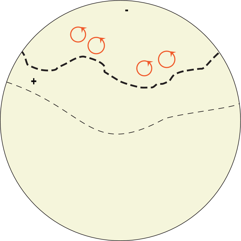
Figure 3: Model of negative polarity flux region fully in the northern hemisphere. The dark dashed line correspond to the PIL of the flux region.

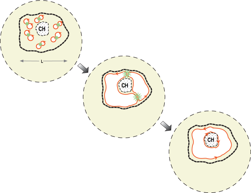
Figure 5: The polarity region of the Figs 3 and 4, but now containing a coronal hole region, indicated by “CH”.

References

- Antiochos (1987) Antiochos, S. K. 1987, ApJ, 312, 886
- Antiochos (1990) Antiochos, S. K. 1990, J. Italian Astron. Soc., 61, 369
- Antiochos et al, (1994) Antiochos, S. K., Dahlburg, R. B., & Klimchuk, J. A. 1994, ApJ, 420, L41
- Antiochos & Dahlburg (1997) Antiochos, S. K. & Dahlburg, R. B. 1997, Sol. Phys., 174, 5
- Antiochos (1998) Antiochos, S. K. 1998, ApJ, 502, L181
- Antiochos et al. (1999) Antiochos, S. K., DeVore, C. R., & Klimchuk, J. A. 1999, ApJ, 510, 485
- Antiochos et al. (2002) Antiochos, S. K., Karpen, J. T., & DeVore, C. R. 2002, ApJ, 575, 578
- Antiochos et al. (2011) Antiochos, S. K., Mikić, Z., Titov, V. S., Lionello, R., & Linker, J. A. 2011, ApJ, 731, 112
- Antiochos et al. (2012) Antiochos, S. K., Linker, J. A., Lionello, R., Mikić, Z., Titov, V. S., & Zurbuchen, T. H. 2011, Space Sci. Rev., 172, 169
- Archontis (2004) Archontis, V. 2004, ApJ, 615, 685
- Berger (1984) Berger, M. A. 1984, Geophys. & Astrophys. Fluid Dynamics, 30, 79
- Berger (1991) Berger, M. A. 1991, A&A, 252, 369
- Berger (2000) Berger, M. A. 2000, Encyclopedia of Astronomy and Astrophysics, ed. P. Murdin, (Bristol: IOP)
- Bieber et al. (1987) Bieber, J. W., Evenson, P. A., & Matthaeus, W. H. 1987, ApJ, 315, 700
- Biskamp (1993) Biskamp, D. 1993, Nonlinear magnetohydrodynamics, Ch. 7, (New York: Cambridge University Press)
- Casini et al. (2003) Casini, R. Lopez Ariste, A., Tomczyk, S., & Lites, B. W. 2003, ApJ, 598, L67
- DeVore (2000) DeVore, C, R. 2000, ApJ, 539, 944
- Duvall & Gizon (2000) Duvall, T. L., Jr. & Gizon, L. 2000, Sol. Phys., 192, 177
- Fan (2001) Fan, Y. 2001, ApJ, 554, L111
- Fang et al. (2012) Fang, F., Manchester, W. B., van der Holst, B. & Abbett, W. 2012, ApJ, 745, 37
- Gizon & Duvall (2003) Gizon, L. & Duvall, T. L., Jr. 2003, in ESA Special Publication, Vol. 517, GONG 2002, Local and Global Helioseismology: The Present and Future, ed. H. Sawaya-Lacoste (Noordwijk: ESA), 43
- Hale (1927) Hale, G. E. 1927, Nature, 119, 708
- Klimchuk (1987) Klimchuk, J. A. 1987, ApJ, 323, 368
- Klimchuk (2006) Klimchuk, J. A. 2006, Sol. Phys., 234, 41, DOI: 10.1007/s11207-006-0055-z
- Kolmogorov (1941) Kolmogorov, A. N. 1941, Dokl. Akad. Nauk. SSSR, 30, 299
- Komm et al. (2007) Komm, R., Howe, R., Hill, F., Miesch, M., Haber, D., & Hindman, B. 2007, ApJ, 667, 571
- Kuckein et al. (2012) Kuckein, C. Martínez Pillet, V., & Centeno, R 2012, A&A, 539, A131
- Kumar & Rust (1996) Kumar, A. & Rust, D. M. 1996, J. Geophys. Res., 101, 15667
- Leake et al. (2010) Leake, J. A., Linton, M. G., & Antiochos, S. K., 2010, ApJ, 722, 550
- Liu & Schuck (2012) Liu Y. & Schuck, P., 2012, ApJ, (in press)
- Harvey (1985) Harvey, K. L. 1985, Aust. J. Phys., 38, 875
- Lau & Finn (1990) Lau, Y.-T. & Finn, J. M. 1990, ApJ, 350, 672
- Leamon et al (1998) Leamon, R. J., Matthaeus, W. H., Smith, C. W., & Wong, H. K. 1998, ApJ, 507, L181
- Leka et al. (1996) Leka, K., Canfield, R., McClymont, A., & van Driel-Gesztelyi, L. 1996, ApJ, 462, 547
- Leroy et al. (1983) Leroy, J.-L., Bommier, V., & Sahal-Brechot, S. 1983, Sol. Phys., 83, 135
- Lin et al. (2005) Lin, Y., Engvold, O., Rouppe van der Voort, L., Wiik, J. E. & Berger, T. E. 2005, Sol. Phys., 226, 239
- Linton et al. (2001) Linton, M. G., Dahlburg, R. B., & Antiochos, S. K. 2001, ApJ, 553, 905
- Magara & Longcope (2003) Magara, T. & Longcope, D. W. 2003, ApJ, 586, 630
- Mancester (2001) Manchester, IV, W. 2001, ApJ, 547, 503
- Martin et al. (1992) Martin, S. F., Marquette, W. H., & Bilimoria, R. 1992, ASP Conf. Ser. 27, The Solar Cycle, ed. K. L. Harvey, (San Francisco: ASP), 53
- Martin (1998) Martin, S. F. 1998, Sol. Phys., 182, 107
- Mackay & van Ballegooijen (2001) Mackay, D. H., & van Ballegooijen, A. A. 2001, ApJ, 560, 445
- Mackay et al. (2010) Mackay, D. H., Karpen, J. T., Ballester, J. L., Schmieder, B., & Aulanier, G. 2010, Space Sci. Rev., 151, 333
- Mikic et al. (1989) Mikic, Z., Schnack, D. D., & van Hoven, G. 1989,ApJ, 338, 1148
- Parker (1972) Parker, E. N. 1972, ApJ, 174, 499
- Parker (1983) Parker, E. N. 1983, ApJ, 264, 642
- Parker (1988) Parker, E. N. 1988, ApJ, 330, 474
- Pevtsov et al. (1995) Pevtsov, A. A., Canfield, R. C., & Metcalf, T. R. 1995, ApJ, 440, L109
- Pevtsov et al. (2003) Pevtsov, A. A., Balasubramaniam, K. S., & Rogers, J. W. 2003, ApJ, 595, 500
- Pevtsov & Balasubramaniam (2003) Pevtsov, A. A. & Balasubramaniam, K. S. 2003, Advances Space Res., 32, 1867
- Pontin et al. (2011) Pontin, D. I., Wilmot-Smith, A. L., Hornig, G., & Galsgaard, K. 2011, A&A, 525, A57
- Priest & Titov (1996) Priest, E. R., & Titov, V. S. 1996, Phil. Trans. R. Soc., 354, 2951
- Qiu et al. (2007) Qiu, J., Hu, Q., Howard, T. A. & Yurchyshyn, V. B. 2007, ApJ, 659, 758
- Rappazzo et al. (2008) Rappazzo, A. F., Velli, M., Einaudi, G., & Dahlburg, R. B. 2008, ApJ, 677, 1348
- Rust (1967) Rust, D. M. 1967, ApJ, 150, 313
- Rust (1994) Rudt, D. M. 1994, Geophys. Res. Lett., 21, 241
- Schrijver et al. (1997) Schrijver, C. J., Title, A. M., van Ballegooijen, A. A., Hagenaar, H. J., and Shine, R. A. 1997, ApJ, 487, 424
- Schrijver et al. (1999) Schrijver, C. J. et al. 1999, Sol. Phys., 198, 325
- Schrijver (2007) Schrijver, C. J. 2007, ApJ, 662, L119
- Sheeley & Warren (2012) Sheeley, N. R. & Warren, H. P. 2012, ApJ, 749, 40
- Seehafer (1990) Seehafer, N. 1990, Sol. Phys., 125, 219
- Su & van Ballegooijen (2012) Su, Y. & van Ballegooijen, A. A. 2012, ApJ, 757, 168
- Sturrock & Uchida (1981) Sturrock, P. A. & Uchida, Y. 1981, ApJ, 246, 331
- Tandberg-Hanssen (1995) Tandberg-Hanssen, E 1995, The Nature of Solar Prominences, (Dordrecht: Kluwer)
- Taylor (1974) Taylor, J. B. 1974, Phys. Rev. Lett., 33, 1139
- Taylor (1986) Taylor, J. B. 1986, Rev. Mod. Phys., 58, 741
- Tian et al. (2005) Tian,L., Alexander, D., & Nightingale, R. 2008, ApJ, 684, 747
- van Ballegooijen (1986) van Ballegooijen, A. A. 1986, ApJ, 311, 1001
- van Ballegooijen & Martens (1989) van Ballegooijen, A. A. & Martens, P. C. H. 1989, ApJ, 343, 971
- van Ballegooijen et al. (1998) van Ballegooijen, A. A., Cartledge, N. P., & Priest, E. R. 1998, ApJ, 501, 866
- van Ballegooijen (2004) van Ballegooijen, A. A. 2004, ApJ, 612, 529
- Vourlidas et al. (2010) Vourlidas A. et al. 2010, Sol. Phys., 261, 53
- Yamada et al. (1990) Yamada, M., Ono, Y., Hayakawa, A., Katsurai, M., & Perkins, F. W. 1990, Phys. Rev. Lett., 65, 721
- Zirker et al. (1997) Zirker, J. B., Martin, S. F., Harvey, K., & Gaizauskas, V. 1997, Sol. Phys., 175, 27