Conway-Gordon type theorem for the complete four-partite graph $K_{3,3,1,1}$

Abstract.

We give a Conway-Gordon type formula for invariants of knots and links in a spatial complete four-partite graph $K_{3,3,1,1}$ in terms of the square of the linking number and the second coefficient of the Conway polynomial. As an application, we show that every rectilinear spatial $K_{3,3,1,1}$ contains a nontrivial Hamiltonian knot.

1. Introduction

Throughout this paper we work in the piecewise linear category. Let $G$ be a finite graph. An embedding $f$ of $G$ into the Euclidean $3$-space ${\mathbb{R}}^{3}$ is called a spatial embedding of $G$ and $f(G)$ is called a spatial graph. We denote the set of all spatial embeddings of $G$ by ${\rm SE}(G)$. We call a subgraph $\gamma$ of $G$ which is homeomorphic to the circle a cycle of $G$ and denote the set of all cycles of $G$ by $\Gamma(G)$. We also call a cycle of $G$ a $k$-cycle if it contains exactly $k$ edges and denote the set of all $k$-cycles of $G$ by $\Gamma_{k}(G)$. In particular, a $k$-cycle is said to be Hamiltonian if $k$ equals the number of all vertices of $G$. For a positive integer $n$, $\Gamma^{(n)}(G)$ denotes the set of all cycles of $G$ ($=\Gamma(G)$) if $n=1$ and the set of all unions of $n$ mutually disjoint cycles of $G$ if $n\geq 2$. For an element $\gamma$ in $\Gamma^{(n)}(G)$ and an element $f$ in ${\rm SE}(G)$, $f(\gamma)$ is none other than a knot in $f(G)$ if $n=1$ and an $n$-component link in $f(G)$ if $n\geq 2$. In particular, we call $f(\gamma)$ a Hamiltonian knot in $f(G)$ if $\gamma$ is a Hamiltonian cycle.

For an edge $e$ of a graph $G$, we denote the subgraph $G\setminus{\rm int}e$ by $G-e$. Let $e=\overline{uv}$ be an edge of $G$ which is not a loop, where $u$ and $v$ are distinct end vertices of $e$. Then we call the graph which is obtained from $G-e$ by identifying $u$ and $v$ the edge contraction of $G$ along $e$ and denote it by $G/e$. A graph $H$ is called a minor of a graph $G$ if there exists a subgraph $G^{\prime}$ of $G$ and the edges $e_{1},e_{2},\ldots,e_{m}$ of $G^{\prime}$ each of which is not a loop such that $H$ is obtained from $G^{\prime}$ by a sequence of edge contractions along $e_{1},e_{2},\ldots,e_{m}$. A minor $H$ of $G$ is called a proper minor if $H$ does not equal $G$. Let ${\mathcal{P}}$ be a property of graphs which is closed under minor reductions; that is, for any graph $G$ which does not have ${\mathcal{P}}$, all minors of $G$ also do not have ${\mathcal{P}}$. A graph $G$ is said to be minor-minimal with respect to ${\mathcal{P}}$ if $G$ has ${\mathcal{P}}$ but all proper minors of $G$ do not have ${\mathcal{P}}$. Then it is known that there exist finitely many minor-minimal graphs with respect to ${\mathcal{P}}$ [21].

Let $K_{m}$ be the complete graph on $m$ vertices, namely the simple graph consisting of $m$ vertices in which every pair of distinct vertices is connected by exactly one edge. Then the following are very famous in spatial graph theory, which are called the Conway-Gordon theorems.

Theorem 1-1.

(Conway-Gordon [4])

1. For any element $f$ in ${\rm SE}(K_{6})$,

   (1.1) $$\sum_{\gamma\in\Gamma^{(2)}(K_{6})}{\rm lk}(f(\gamma))\equiv 1\pmod{2},$$

   where ${\rm lk}$ denotes the linking number.

2. For any element $f$ in ${\rm SE}(K_{7})$,

   (1.2) $$\sum_{\gamma\in\Gamma_{7}(K_{7})}a_{2}(f(\gamma))\equiv 1\pmod{2},$$

   where $a_{2}$ denotes the second coefficient of the Conway polynomial.

A graph is said to be intrinsically linked if for any element $f$ in ${\rm SE}(G)$, there exists an element $\gamma$ in $\Gamma^{(2)}(G)$ such that $f(\gamma)$ is a nonsplittable $2$-component link, and to be intrinsically knotted if for any element $f$ in ${\rm SE}(G)$, there exists an element $\gamma$ in $\Gamma(G)$ such that $f(\gamma)$ is a nontrivial knot. Theorem 1-1 implies that $K_{6}$ (resp. $K_{7}$) is intrinsically linked (resp. knotted). Moreover, the intrinsic linkedness (resp. knottedness) is closed under minor reductions [16] (resp. [5]), and $K_{6}$ (resp. $K_{7}$) is minor-minimal with respect to the intrinsically linkedness [23] (resp. knottedness [14]).

A $\triangle Y$-exchange is an operation to obtain a new graph $G_{Y}$ from a graph $G_{\triangle}$ by removing all edges of a $3$-cycle $\triangle$ of $G_{\triangle}$ with the edges $\overline{uv},\overline{vw}$ and $\overline{wu}$, and adding a new vertex $x$ and connecting it to each of the vertices $u,v$ and $w$ as illustrated in Fig. 1.1 (we often denote $\overline{ux}\cup\overline{vx}\cup\overline{wx}$ by $Y$). A $Y\triangle$-exchange is the reverse of this operation. We call the set of all graphs obtained from a graph $G$ by a finite sequence of $\triangle Y$ and $Y\triangle$-exchanges the $G$-family and denote it by ${\mathcal{F}}(G)$. In particular, we denote the set of all graphs obtained from $G$ by a finite sequence of $\triangle Y$-exchanges by ${\mathcal{F}}_{\triangle}(G)$. For example, it is well known that the $K_{6}$-family consists of exactly seven graphs as illustrated in Fig. 1.2, where an arrow between two graphs indicates the application of a single $\triangle Y$-exchange. Note that ${\mathcal{F}}_{\triangle}(K_{6})={\mathcal{F}}(K_{6})\setminus\left\{P_{7}\right\}$. Since $P_{10}$ is isomorphic to the Petersen graph, the $K_{6}$-family is also called the Petersen family. It is also well known that the $K_{7}$-family consists of exactly twenty graphs, and there exist exactly six graphs in the $K_{7}$-family each of which does not belong to ${\mathcal{F}}_{\triangle}(K_{7})$. Then the intrinsic linkedness and the intrinsic knottedness behave well under $\triangle Y$-exchanges as follows.

Proposition 1-2.

(Sachs [23])

1. If $G_{\triangle}$ is intrinsically linked, then $G_{Y}$ is also intrinsically linked.

2. If $G_{\triangle}$ is intrinsically knotted, then $G_{Y}$ is also intrinsically knotted.

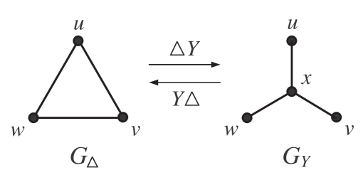
Figure 1.1.

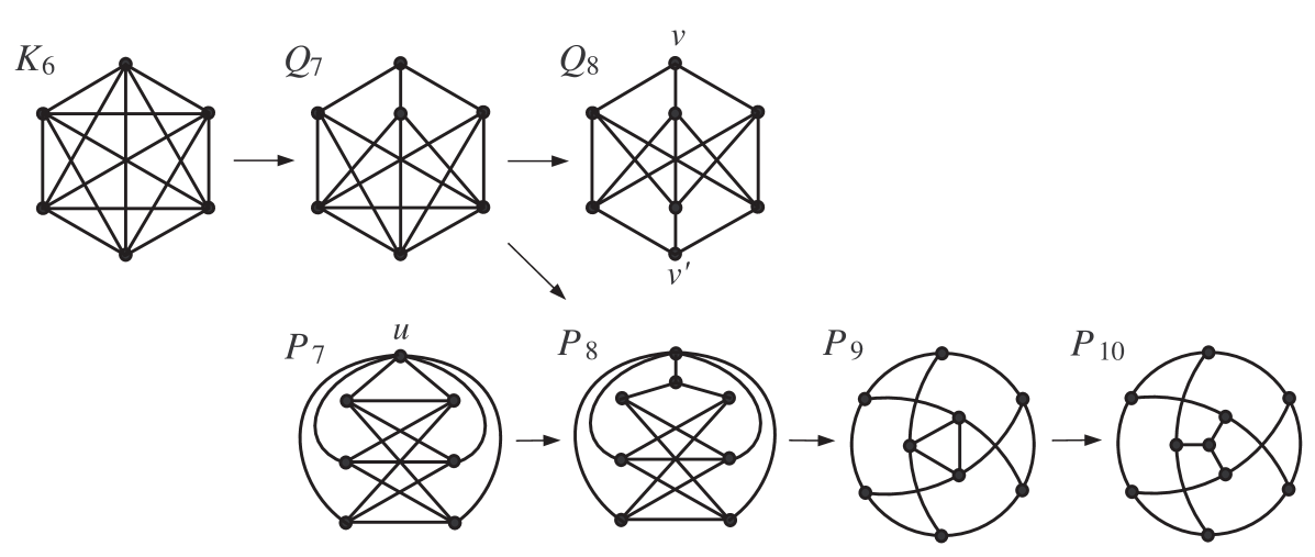
Figure 1.2.

Proposition 1-2 implies that any element in ${\mathcal{F}}_{\triangle}(K_{6})$ (resp. ${\mathcal{F}}_{\triangle}(K_{7})$) is intrinsically linked (resp. knotted). In particular, Robertson-Seymour-Thomas showed that the set of all minor-minimal intrinsically linked graphs equals the $K_{6}$-family, so the converse of Proposition 1-2 (1) is also true [22]. On the other hand, it is known that any element in ${\mathcal{F}}_{\triangle}(K_{7})$ is minor-minimal with respect to the intrinsic knottedness [13], but any element in ${\mathcal{F}}(K_{7})\setminus{\mathcal{F}}_{\triangle}(K_{7})$ is not intrinsically knotted [6], [11], [10], so the converse of Proposition 1-2 (2) is not true. Moreover, there exists a minor-minimal intrinsically knotted graph which does not belong to ${\mathcal{F}}_{\triangle}(K_{7})$ as follows. Let $K_{n_{1},n_{2},\ldots,n_{m}}$ be the complete $m$-partite graph, namely the simple graph whose vertex set can be decomposed into $m$ mutually disjoint nonempty sets $V_{1},V_{2},\ldots,V_{m}$ where the number of elements in $V_{i}$ equals $n_{i}$ such that no two vertices in $V_{i}$ are connected by an edge and every pair of vertices in the distinct sets $V_{i}$ and $V_{j}$ is connected by exactly one edge, see Fig. 1.3 which illustrates $K_{3,3}$, $K_{3,3,1}$ and $K_{3,3,1,1}$. Note that $K_{3,3,1}$ is isomorphic to $P_{7}$ in the $K_{6}$-family, namely $K_{3,3,1}$ is a minor-minimal intrinsically linked graph. On the other hand, Motwani-Raghunathan-Saran claimed in [14] that it may be proven that $K_{3,3,1,1}$ is intrinsically knotted by using the same technique of Theorem 1-1, namely, by showing that for any element in ${\rm SE}(K_{3,3,1,1})$, the sum of $a_{2}$ over all of the Hamiltonian knots is always congruent to one modulo two. But Kohara-Suzuki showed in [13] that the claim did not hold; that is, the sum of $a_{2}$ over all of the Hamiltonian knots is dependent to each element in ${\rm SE}(K_{3,3,1,1})$. Actually, they demonstrated the specific two elements $f_{1}$ and $f_{2}$ in ${\rm SE}(K_{3,3,1,1})$ as illustrated in Fig. 1.4. Here $f_{1}(K_{3,3,1,1})$ contains exactly one nontrivial knot $f_{1}(\gamma_{0})$ ($=$ a trefoil knot, $a_{2}=1$) which is drawn by bold lines, where $\gamma_{0}$ is an element in $\Gamma_{8}(K_{3,3,1,1})$, and $f_{2}(K_{3,3,1,1})$ contains exactly two nontrivial knots $f_{2}(\gamma_{1})$ and $f_{2}(\gamma_{2})$ ($=$ two trefoil knots) which are drawn by bold lines, where $\gamma_{1}$ and $\gamma_{2}$ are elements in $\Gamma_{8}(K_{3,3,1,1})$. Thus the situation of the case of $K_{3,3,1,1}$ is different from the case of $K_{7}$. By using another technique different from Conway-Gordon’s, Foisy proved the following.

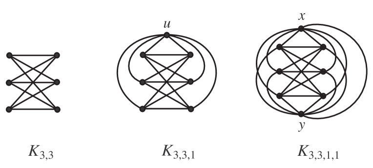
Figure 1.3.

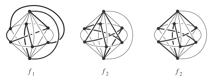
Figure 1.4.

Theorem 1-3.

(Foisy [7]) For any element $f$ in ${\rm SE}(K_{3,3,1,1})$, there exists an element $\gamma$ in $\cup_{k=4}^{8}\Gamma_{k}(K_{3,3,1,1})$ such that $a_{2}(f(\gamma))\equiv 1\pmod{2}$.

Theorem 1-3 implies that $K_{3,3,1,1}$ is intrinsically knotted. Moreover, Proposition 1-2 (2) and Theorem 1-3 implies that any element $G$ in ${\mathcal{F}}_{\triangle}(K_{3,3,1,1})$ is also intrinsically knotted. It is known that there exist exactly twenty six elements in ${\mathcal{F}}_{\triangle}(K_{3,3,1,1})$. Since Kohara-Suzuki pointed out that each of the proper minors of $G$ is not intrinsically knotted [13], it follows that any element in ${\mathcal{F}}_{\triangle}(K_{3,3,1,1})$ is minor-minimal with respect to the intrinsic knottedness. Note that a $\triangle Y$-exchange does not change the number of edges of a graph. Since $K_{7}$ and $K_{3,3,1,1}$ have different numbers of edges, the families ${\mathcal{F}}_{\triangle}(K_{7})$ and ${\mathcal{F}}_{\triangle}(K_{3,3,1,1})$ are disjoint.

Our first purpose in this article is to refine Theorem 1-3 by giving a kind of Conway-Gordon type formula for $K_{3,3,1,1}$ not over ${\mathbb{Z}}_{2}$, but integers ${\mathbb{Z}}$. In the following, $\Gamma_{k,l}^{(2)}(G)$ denotes the set of all unions of two disjoint cycles of a graph $G$ consisting of a $k$-cycle and an $l$-cycle, and $x$ and $y$ denotes the two vertices of $K_{3,3,1,1}$ with valency seven. Then we have the following.

Theorem 1-4.

1. For any element $f$ in ${\rm SE}(K_{3,3,1,1})$,

   $$4\sum_{\gamma\in\Gamma_{8}(K_{3,3,1,1})}a_{2}(f(\gamma))-4\sum_{\begin{subarray}{c}{\gamma\in\Gamma_{7}(K_{3,3,1,1})}\\ {\left\{x,y\right\}\not\subset\gamma}\end{subarray}}a_{2}(f(\gamma))$$

   $$-4\sum_{\gamma\in\Gamma_{6}^{\prime}}a_{2}(f(\gamma))-4\sum_{\begin{subarray}{c}{\gamma\in\Gamma_{5}(K_{3,3,1,1})}\\ {\left\{x,y\right\}\not\subset\gamma}\end{subarray}}a_{2}(f(\gamma))$$

   $$= \sum_{\lambda\in\Gamma_{3,5}^{(2)}(K_{3,3,1,1})}{\rm lk}(f(\lambda))^{2}+2\sum_{\lambda\in\Gamma_{4,4}^{(2)}(K_{3,3,1,1})}{\rm lk}(f(\lambda))^{2}-18,$$

   where $\Gamma_{6}^{\prime}$ is a specific proper subset of $\Gamma_{6}(K_{3,3,1,1})$ which does not depend on $f$, see (2).

2. For any element $f$ in ${\rm SE}(K_{3,3,1,1})$,

   (1.4) $$\sum_{\lambda\in\Gamma_{3,5}^{(2)}(K_{3,3,1,1})}{\rm lk}(f(\lambda))^{2}+2\sum_{\lambda\in\Gamma_{4,4}^{(2)}(K_{3,3,1,1})}{\rm lk}(f(\lambda))^{2}\geq 22.$$

We prove Theorem 1-4 in the next section. By combining Theorem 1-4 (1) and (2), we immediately have the following.

Corollary 1-5.

For any element $f$ in ${\rm SE}(K_{3,3,1,1})$,

(1.5) $$\sum_{\gamma\in\Gamma_{8}(K_{3,3,1,1})}a_{2}(f(\gamma))-\sum_{\begin{subarray}{c}{\gamma\in\Gamma_{7}(K_{3,3,1,1})}\\ {\left\{x,y\right\}\not\subset\gamma}\end{subarray}}a_{2}(f(\gamma))$$

$$-\sum_{\gamma\in\Gamma_{6}^{\prime}}a_{2}(f(\gamma))-\sum_{\begin{subarray}{c}{\gamma\in\Gamma_{5}(K_{3,3,1,1})}\\ {\left\{x,y\right\}\not\subset\gamma}\end{subarray}}a_{2}(f(\gamma))\geq 1.$$

Corollary 1-5 gives an alternative proof of the fact that $K_{3,3,1,1}$ is intrinsically knotted. Moreover, Corollary 1-5 refines Theorem 1-3 by identifying the cycles that might be nontrivial knots in $f(K_{3,3,1,1})$.

Remark 1-6.

We see the left side of (1.5) is not always congruent to one modulo two by considering two elements $f_{1}$ and $f_{2}$ in ${\rm SE}(K_{3,3,1,1})$ as illustrated in Fig. 1.4. Thus Corollary 1-5 shows that the argument over ${\mathbb{Z}}$ has a nice advantage. In particular, $f_{1}$ gives the best possibility for (1.5), and therefore for (1.4) by Theorem 1-4 (1). Actually $f_{1}(K_{3,3,1,1})$ contains exactly fourteen nontrivial links all of which are Hopf links, where the six of them are the images of elements in $\Gamma_{3,5}^{(2)}(K_{3,3,1,1})$ by $f_{1}$ and the eight of them are the images of elements in $\Gamma_{4,4}^{(2)}(K_{3,3,1,1})$ by $f_{1}$.

As we said before, any element $G$ in ${\mathcal{F}}_{\triangle}(K_{7})\cup{\mathcal{F}}_{\triangle}(K_{3,3,1,1})$ is a minor-minimal intrinsically knotted graph. If $G$ belongs to ${\mathcal{F}}_{\triangle}(K_{7})$, then it is known that Conway-Gordon type formula over ${\mathbb{Z}}_{2}$ as in Theorem 1-1 also holds for $G$ as follows.

Theorem 1-7.

(Nikkuni-Taniyama [18]) Let $G$ be an element in ${\mathcal{F}}_{\triangle}(K_{7})$. Then, there exists a map $\omega$ from $\Gamma(G)$ to ${\mathbb{Z}}_{2}$ such that for any element $f$ in ${\rm SE}(G)$,

$$\sum_{\gamma\in\Gamma(G)}\omega(\gamma)a_{2}(f(\gamma))\equiv 1\pmod{2}.$$

Namely, for any element $G$ in ${\mathcal{F}}_{\triangle}(K_{7})$, there exists a subset $\Gamma$ of $\Gamma(G)$ which depends on only $G$ such that for any element $f$ in ${\rm SE}(G)$, the sum of $a_{2}$ over all of the images of the elements in $\Gamma$ by $f$ is odd. On the other hand, if $G$ belongs to ${\mathcal{F}}_{\triangle}(K_{3,3,1,1})$, we have a Conway-Gordon type formula over ${\mathbb{Z}}$ for $G$ as in Corollary 1-5 as follows. We prove it in section $3$.

Theorem 1-8.

Let $G$ be an element in ${\mathcal{F}}_{\triangle}(K_{3,3,1,1})$. Then, there exists a map $\omega$ from $\Gamma(G)$ to ${\mathbb{Z}}$ such that for any element $f$ in ${\rm SE}(G)$,

$$\sum_{\gamma\in\Gamma(G)}\omega(\gamma)a_{2}(f(\gamma))\geq 1.$$

Our second purpose in this article is to give an application of Theorem 1-4 to the theory of rectilinear spatial graphs. A spatial embedding $f$ of a graph $G$ is said to be rectilinear if for any edge $e$ of $G$, $f(e)$ is a straight line segment in ${\mathbb{R}}^{3}$. We denote the set of all rectilinear spatial embeddings of $G$ by ${\rm RSE}(G)$. We can see that any simple graph has a rectilinear spatial embedding by taking all of the vertices on the spatial curve $(t,t^{2},t^{3})$ in ${\mathbb{R}}^{3}$ and connecting every pair of two adjacent vertices by a straight line segment. Rectilinear spatial graphs appear in polymer chemistry as a mathematical model for chemical compounds, see [1] for example. Then by an application of Theorem 1-4, we have the following.

Theorem 1-9.

For any element $f$ in ${\rm RSE}(K_{3,3,1,1})$,

$$\sum_{\gamma\in\Gamma_{8}(K_{3,3,1,1})}a_{2}(f(\gamma))\geq 1.$$

We prove Theorem 1-9 in section $4$. As a corollary of Theorem 1-9, we immediately have the following.

Corollary 1-10.

For any element $f$ in ${\rm RSE}(K_{3,3,1,1})$, there exists a Hamiltonian cycle $\gamma$ of $K_{3,3,1,1}$ such that $f(\gamma)$ is a nontrivial knot with $a_{2}(f(\gamma))>0$.

Corollary 1-10 is an affirmative answer to the question of Foisy-Ludwig [9, Question 5.8] which asks whether the image of every rectilinear spatial embedding of $K_{3,3,1,1}$ always contains a nontrivial Hamiltonian knot.

Remark 1-11.

1. In [9, Question 5.8], Foisy-Ludwig also asked that whether the image of every spatial embedding of $K_{3,3,1,1}$ (which may not be rectilinear) always contains a nontrivial Hamiltonian knot. As far as the authors know, it is still open.

2. In addition to the elements in ${\mathcal{F}}_{\triangle}(K_{7})\cup{\mathcal{F}}_{\triangle}(K_{3,3,1,1})$, many minor-minimal intrinsically knotted graph are known [8], [10]. In particular, it has been announced by Goldberg-Mattman-Naimi that all of the thirty two elements in ${\mathcal{F}}(K_{3,3,1,1})\setminus{\mathcal{F}}_{\triangle}(K_{3,3,1,1})$ are minor-minimal intrinsically knotted graphs [10]. Note that their method is based on Foisy’s idea in the proof of Theorem 1-3 with the help of a computer.

2. Conway-Gordon type formula for $K_{3,3,1,1}$

To prove Theorem 1-4, we recall a Conway-Gordon type formula over ${\mathbb{Z}}$ for a graph in the $K_{6}$-family which is as below.

Theorem 2-1.

Let $G$ be an element in ${\mathcal{F}}(K_{6})$. Then there exist a map $\omega$ from $\Gamma(G)$ to ${\mathbb{Z}}$ such that for any element $f$ in ${\rm SE}(G)$,

(2.1) $$2\sum_{\gamma\in\Gamma(G)}\omega(\gamma)a_{2}(f(\gamma))=\sum_{\gamma\in\Gamma^{(2)}(G)}{\rm lk}(f(\gamma))^{2}-1.$$

We remark here that Theorem 2-1 was shown by Nikkuni (for the case $G=K_{6}$) [17], O’Donnol ($G=P_{7}$) [19] and Nikkuni-Taniyama (for the others) [18]. In particular, we use the following explicit formulae for $Q_{8}$ and $P_{7}$ in the proof of Theorem 1-4. For the other cases, see Hashimoto-Nikkuni [12].

Theorem 2-2.

1. (Hashimoto-Nikkuni [12]) For any element $f$ in ${\rm SE}(Q_{8})$,

   $$2\sum_{\gamma\in\Gamma_{7}(P_{7})}a_{2}(f(\gamma))+2\sum_{\begin{subarray}{c}{\gamma\in\Gamma_{6}(Q_{8})}\\ {v,v^{\prime}\not\in\gamma}\end{subarray}}a_{2}(f(\gamma))-2\sum_{\begin{subarray}{c}{\gamma\in\Gamma_{6}(Q_{8})}\\ {\gamma\cap\{v,v^{\prime}\}\neq\emptyset}\end{subarray}}a_{2}(f(\gamma))$$

   $$= \sum_{\gamma\in\Gamma_{4,4}^{(2)}(Q_{8})}{\rm lk}(f(\gamma))^{2}-1,$$

   where $v$ and $v^{\prime}$ are exactly two vertices of $Q_{8}$ with valency three.

2. (O’Donnol [19]) For any element $f$ in ${\rm SE}(P_{7})$,

   $$2\sum_{\gamma\in\Gamma_{7}(P_{7})}a_{2}(f(\gamma))-4\sum_{\begin{subarray}{c}{\gamma\in\Gamma_{6}(P_{7})}\\ {u\not\in\gamma}\end{subarray}}a_{2}(f(\gamma))-2\sum_{\gamma\in\Gamma_{5}(P_{7})}a_{2}(f(\gamma))$$

   $$= \sum_{\gamma\in\Gamma_{3,4}^{(2)}(P_{7})}{\rm lk}(f(\gamma))^{2}-1,$$

   where $u$ is the vertex of $P_{7}$ with valency six.

By taking the modulo two reduction of (2.1), we immediately have the following fact containing Theorem 1-1 (1).

Corollary 2-3.

(Sachs [23], Taniyama-Yasuhara [24]) Let $G$ be an element in ${\mathcal{F}}(K_{6})$. Then, for any element $f$ in ${\rm SE}(G)$,

$$\sum_{\gamma\in\Gamma^{(2)}(G)}{\rm lk}(f(\gamma))\equiv 1\pmod{2}.$$

Now we give labels for the vertices of $K_{3,3,1,1}$ as illustrated in the left figure in Fig. 2.1. We also call the vertices $1,3,5$ and $2,4,6$ the black vertices and the white vertices, respectively. We regard $K_{3,3}$ as the subgraph of $K_{3,3,1,1}$ induced by all of the white and black vertices. Let $G_{x}$ and $G_{y}$ be two subgraphs of $K_{3,3,1,1}$ as illustrated in Fig. 2.1 (1) and (2), respectively. Since each of $G_{x}$ and $G_{y}$ is isomorphic to $P_{7}$, by applying Theorem 2-2 (2) to $f|_{G_{x}}$ and $f|_{G_{y}}$ for an element $f$ in ${\rm SE}(K_{3,3,1,1})$, it follows that

$$2\sum_{\gamma\in\Gamma_{7}(G_{x})}a_{2}(f(\gamma))-4\sum_{\gamma\in\Gamma_{6}(K_{3,3})}a_{2}(f(\gamma))-2\sum_{\gamma\in\Gamma_{5}(G_{x})}a_{2}(f(\gamma))$$

$$= \sum_{\gamma\in\Gamma_{3,4}^{(2)}(G_{x})}{\rm lk}(f(\gamma))^{2}-1,$$

$$2\sum_{\gamma\in\Gamma_{7}(G_{y})}a_{2}(f(\gamma))-4\sum_{\gamma\in\Gamma_{6}(K_{3,3})}a_{2}(f(\gamma))-2\sum_{\gamma\in\Gamma_{5}(G_{y})}a_{2}(f(\gamma))$$

$$= \sum_{\gamma\in\Gamma_{3,4}^{(2)}(G_{y})}{\rm lk}(f(\gamma))^{2}-1.$$

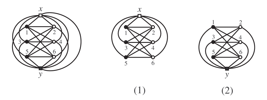
Figure 2.1. (1) $G_{x}$, (2) $G_{y}$

Let $\gamma$ be an element in $\Gamma(K_{3,3,1,1})$ which is a $8$-cycle or a $6$-cycle containing $x$ and $y$. Then we say that $\gamma$ is of Type A if the neighbor vertices of $x$ in $\gamma$ consist of both a black vertex and a white vertex (if and only if the neighbor vertices of $y$ in $\gamma$ consist of both a black vertex and a white vertex), of Type B if the neighbor vertices of $x$ in $\gamma$ consist of only black (resp. white) vertices and the neighbor vertices of $y$ in $\gamma$ consist of only white (resp. black) vertices, and of Type C if $\gamma$ contains the edge $\overline{xy}$. Moreover, we say that an element $\gamma$ in $\Gamma_{6}(K_{3,3,1,1})$ containing $x$ and $y$ is of Type D if the neighbor vertices of $x$ and $y$ in $\gamma$ consist of only black or only white vertices. Note that any element in $\Gamma_{8}(K_{3,3,1,1})$ is of Type A, B or C, and any element in $\Gamma_{6}(K_{3,3,1,1})$ containing $x$ and $y$ is of Type A, B, C or D. On the other hand, let $\lambda$ be an element in $\Gamma_{4,4}^{(2)}(K_{3,3,1,1})$. Then we say that $\lambda$ is of Type A if $\lambda$ does not contain the edge $\overline{xy}$ and both $x$ and $y$ are contained in either connected component of $\lambda$, of Type B if $x$ and $y$ are contained in different connected components of $\lambda$, and of Type C if $\lambda$ contains the edge $\overline{xy}$. Note that any element in $\Gamma_{4,4}^{(2)}(K_{3,3,1,1})$ is of Type A, B or C. Then the following three lemmas hold.

Lemma 2-4.

For any element $f$ in ${\rm SE}(K_{3,3,1,1})$,

$$\sum_{\lambda\in\Gamma_{3,5}^{(2)}(K_{3,3,1,1})}{\rm lk}(f(\lambda))^{2}+2\sum_{\begin{subarray}{c}{\lambda\in\Gamma_{4,4}^{(2)}(K_{3,3,1,1})}\\ {\rm Type\ A}\end{subarray}}{\rm lk}(f(\lambda))^{2}$$

$$= 4\sum_{\begin{subarray}{c}{\gamma\in\Gamma_{8}(K_{3,3,1,1})}\\ {\rm Type\ A}\end{subarray}}a_{2}(f(\gamma))-4\left\{\sum_{\gamma\in\Gamma_{7}(G_{x})}a_{2}(f(\gamma))+\sum_{\gamma\in\Gamma_{7}(G_{y})}a_{2}(f(\gamma))\right\}$$

$$+8\sum_{\gamma\in\Gamma_{6}(K_{3,3})}a_{2}(f(\gamma))-4\sum_{\begin{subarray}{c}{\gamma\in\Gamma_{6}(K_{3,3,1,1})}\\ x,y\in\gamma,\ {\rm Type\ A}\end{subarray}}a_{2}(f(\gamma))$$

$$-4\left\{\sum_{\gamma\in\Gamma_{5}(G_{x})}a_{2}(f(\gamma))+\sum_{\gamma\in\Gamma_{5}(G_{y})}a_{2}(f(\gamma))\right\}+10.$$

Proof.

For $i=1,3,5$ and $j=2,4,6$, let us consider subgraphs $F_{x}^{(ij)}=(G_{x}-\overline{ij})\cup\overline{iy}\cup\overline{jy}$ and $F_{y}^{(ij)}=(G_{y}-\overline{ij})\cup\overline{ix}\cup\overline{jx}$ of $K_{3,3,1,1}$ as illustrated in Fig. 2.2 (1) and (2), respectively. Since each of $F_{x}^{(ij)}$ and $F_{y}^{(ij)}$ is homeomorphic to $P_{7}$, by applying Theorem 2-2 (2) to $f|_{F_{x}^{(ij)}}$, it follows that

$$\sum_{\begin{subarray}{c}{\lambda=\gamma\cup\gamma^{\prime}\in\Gamma_{3,5}^{(2)}(F_{x}^{(ij)})}\\ \gamma\in\Gamma_{3}(F_{x}^{(ij)}),\ \gamma^{\prime}\in\Gamma_{5}(F_{x}^{(ij)})\\ x\in\gamma,\ y\in\gamma^{\prime}\end{subarray}}{\rm lk}(f(\lambda))^{2}+\sum_{\begin{subarray}{c}{\lambda=\gamma\cup\gamma^{\prime}\in\Gamma_{4,4}^{(2)}(F_{x}^{(ij)})}\\ x,y\in\gamma^{\prime}\end{subarray}}{\rm lk}(f(\lambda))^{2}$$

$$+\sum_{\begin{subarray}{c}{\lambda=\gamma\cup\gamma^{\prime}\in\Gamma_{3,4}^{(2)}(G_{x})}\\ \gamma\in\Gamma_{3}(G_{x}),\ \gamma^{\prime}\in\Gamma_{4}(G_{x})\\ \overline{ij}\not\subset\lambda,\ x\in\gamma\end{subarray}}{\rm lk}(f(\lambda))^{2}$$

$$= 2\left\{\sum_{\gamma\in\Gamma_{8}(F_{x}^{(ij)})}a_{2}(f(\gamma))+\sum_{\begin{subarray}{c}{\gamma\in\Gamma_{7}(G_{x})}\\ \overline{ij}\not\subset\gamma\end{subarray}}a_{2}(f(\gamma))\right\}$$

$$-4\left\{\sum_{\begin{subarray}{c}{\gamma\in\Gamma_{7}(F_{x}^{(ij)})}\\ x\not\in\gamma,\ y\in\gamma\end{subarray}}a_{2}(f(\gamma))+\sum_{\begin{subarray}{c}{\gamma\in\Gamma_{6}(K_{3,3})}\\ \overline{ij}\not\subset\gamma\end{subarray}}a_{2}(f(\gamma))\right\}$$

$$-2\left\{\sum_{\begin{subarray}{c}{\gamma\in\Gamma_{6}(F_{x}^{(ij)})}\\ x,y\in\gamma\end{subarray}}a_{2}(f(\gamma))+\sum_{\begin{subarray}{c}{\gamma\in\Gamma_{5}(G_{x})}\\ \overline{ij}\not\subset\gamma\end{subarray}}a_{2}(f(\gamma))\right\}+1.$$

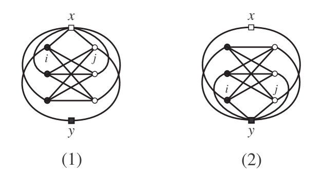
Figure 2.2. (1) $F_{x}^{(ij)}$, (2) $F_{y}^{(ij)}$ $(i=1,3,5,\ j=2,4,6)$

Let us take the sum of both sides of (2) over $i=1,3,5$ and $j=2,4,6$. For an element $\gamma$ in $\Gamma_{8}(K_{3,3,1,1})$ of Type A, there uniquely exists $F_{x}^{(ij)}$ containing $\gamma$. This implies that

(2.6) $$\sum_{i,j}\left(\sum_{\gamma\in\Gamma_{8}(F_{x}^{(ij)})}a_{2}(f(\gamma))\right)=\sum_{\begin{subarray}{c}{\gamma\in\Gamma_{8}(K_{3,3,1,1})}\\ {\rm Type\ A}\end{subarray}}a_{2}(f(\gamma)).$$

For an element $\gamma$ of $\Gamma_{7}(G_{x})$, there exist exactly four edges of $K_{3,3}$ which are not contained in $\gamma$. Thus $\gamma$ is common for exactly four $F_{x}^{(ij)}$’s. This implies that

(2.7) $$\sum_{i,j}\left(\sum_{\begin{subarray}{c}{\gamma\in\Gamma_{7}(G_{x})}\\ \overline{ij}\not\subset\gamma\end{subarray}}a_{2}(f(\gamma))\right)=4\sum_{\Gamma_{7}(G_{x})}a_{2}(f(\gamma)).$$

For an element $\gamma$ in $\Gamma_{7}(G_{y})$, there uniquely exists $F_{x}^{(ij)}$ containing $\gamma$. This implies that

(2.8) $$\sum_{i,j}\left(\sum_{\begin{subarray}{c}{\gamma\in\Gamma_{7}(F_{x}^{(ij)})}\\ x\not\in\gamma,\ y\in\gamma\end{subarray}}a_{2}(f(\gamma))\right)=\sum_{\gamma\in\Gamma_{7}(G_{y})}a_{2}(f(\gamma)).$$

For an element $\gamma$ in $\Gamma_{6}(K_{3,3})$, there exist exactly three edges of $K_{3,3}$ which are not contained in $\gamma$. Thus $\gamma$ is common for exactly three $F_{x}^{(ij)}$’s. This implies that

(2.9) $$\sum_{i,j}\left(\sum_{\begin{subarray}{c}{\gamma\in\Gamma_{6}(K_{3,3})}\\ \overline{ij}\not\subset\gamma\end{subarray}}a_{2}(f(\gamma))\right)=3\sum_{\gamma\in\Gamma_{6}(K_{3,3})}a_{2}(f(\gamma)).$$

For an element $\gamma$ in $\Gamma_{6}(K_{3,3,1,1})$ containing $x$ and $y$, if $\gamma$ is of Type A, then there uniquely exists $F_{x}^{(ij)}$ containing $\gamma$. This implies that

(2.10) $$\sum_{i,j}\left(\sum_{\begin{subarray}{c}{\gamma\in\Gamma_{6}(F_{x}^{(ij)})}\\ x,y\in\gamma\end{subarray}}a_{2}(f(\gamma))\right)=\sum_{\begin{subarray}{c}{\gamma\in\Gamma_{6}(K_{3,3,1,1})}\\ x,y\in\gamma,\ {\rm Type\ A}\end{subarray}}a_{2}(f(\gamma)).$$

For an element $\gamma$ in $\Gamma_{5}(G_{x})$, there exist exactly six edges of $K_{3,3}$ which are not contained in $\gamma$. Thus $\gamma$ is common for exactly six $F_{x}^{(ij)}$’s. This implies that

(2.11) $$\sum_{i,j}\left(\sum_{\begin{subarray}{c}{\gamma\in\Gamma_{5}(G_{x})}\\ \overline{ij}\not\subset\gamma\end{subarray}}a_{2}(f(\gamma))\right)=6\sum_{\gamma\in\Gamma_{5}(G_{x})}a_{2}(f(\gamma)).$$

For an element $\lambda=\gamma\cup\gamma^{\prime}$ in $\Gamma_{3,5}^{(2)}(K_{3,3,1,1})$ where $\gamma$ is a $3$-cycle and $\gamma^{\prime}$ is a $5$-cycle, if $\gamma$ contains $x$ and $\gamma^{\prime}$ contains $y$, then there uniquely exists $F_{x}^{(ij)}$ containing $\lambda$. This implies that

$$\sum_{i,j}\left(\sum_{\begin{subarray}{c}{\lambda=\gamma\cup\gamma^{\prime}\in\Gamma_{3,5}^{(2)}(F_{x}^{(ij)})}\\ \gamma\in\Gamma_{3}(F_{x}^{(ij)}),\ \gamma^{\prime}\in\Gamma_{5}(F_{x}^{(ij)})\\ x\in\gamma,\ y\in\gamma^{\prime}\end{subarray}}{\rm lk}(f(\lambda))^{2}\right)$$

$$= \sum_{\begin{subarray}{c}{\lambda=\gamma\cup\gamma^{\prime}\in\Gamma_{3,5}^{(2)}(K_{3,3,1,1})}\\ \gamma\in\Gamma_{3}(K_{3,3,1,1}),\ \gamma^{\prime}\in\Gamma_{5}(K_{3,3,1,1})\\ x\in\gamma,\ y\in\gamma^{\prime}\end{subarray}}{\rm lk}(f(\lambda))^{2}.$$

For an element $\lambda$ in $\Gamma_{4,4}^{(2)}(K_{3,3,1,1})$ of Type A, there uniquely exists $F_{x}^{(ij)}$ containing $\lambda$. This implies that

(2.13) $$\sum_{i,j}\left(\sum_{\begin{subarray}{c}{\lambda=\gamma\cup\gamma^{\prime}\in\Gamma_{4,4}^{(2)}(F_{x}^{(ij)})}\\ x,y\in\gamma^{\prime}\end{subarray}}{\rm lk}(f(\lambda))^{2}\right)=\sum_{\begin{subarray}{c}{\lambda\in\Gamma_{4,4}^{(2)}(K_{3,3,1,1})}\\ {\rm Type\ A}\end{subarray}}{\rm lk}(f(\lambda))^{2}.$$

For an element $\lambda$ in $\Gamma_{3,4}^{(2)}(G_{x})$, there exist exactly four edges of $K_{3,3}$ which are not contained in $\lambda$. Thus $\lambda$ is common for exactly four $F_{x}^{(ij)}$’s. This implies that

(2.14) $$\sum_{i,j}\left(\sum_{\begin{subarray}{c}{\lambda=\gamma\cup\gamma^{\prime}\in\Gamma_{3,4}^{(2)}(G_{x})}\\ \gamma\in\Gamma_{3}(G_{x}),\ \gamma^{\prime}\in\Gamma_{4}(G_{x})\\ \overline{ij}\not\subset\lambda,\ x\in\gamma\end{subarray}}{\rm lk}(f(\lambda))^{2}\right)=4\sum_{\lambda\in\Gamma_{3,4}^{(2)}(G_{x})}{\rm lk}(f(\lambda))^{2}.$$

Thus by (2), (2.6), (2.7), (2.8), (2.9), (2.10), (2.11), (2), (2.13) and (2.14), we have

$$\sum_{\begin{subarray}{c}{\lambda=\gamma\cup\gamma^{\prime}\in\Gamma_{3,5}^{(2)}(K_{3,3,1,1})}\\ \gamma\in\Gamma_{3}(K_{3,3,1,1}),\ \gamma^{\prime}\in\Gamma_{5}(K_{3,3,1,1})\\ x\in\gamma,\ y\in\gamma^{\prime}\end{subarray}}{\rm lk}(f(\lambda))^{2}+\sum_{\begin{subarray}{c}{\lambda\in\Gamma_{4,4}^{(2)}(K_{3,3,1,1})}\\ {\rm Type\ A}\end{subarray}}{\rm lk}(f(\lambda))^{2}$$

$$+4\sum_{\lambda\in\Gamma_{3,4}^{(2)}(G_{x})}{\rm lk}(f(\lambda))^{2}$$

$$= 2\sum_{\begin{subarray}{c}{\gamma\in\Gamma_{8}(K_{3,3,1,1})}\\ {\rm Type\ A}\end{subarray}}a_{2}(f(\gamma))+8\sum_{\gamma\in\Gamma_{7}(G_{x})}a_{2}(f(\gamma))-4\sum_{\gamma\in\Gamma_{7}(G_{y})}a_{2}(f(\gamma))$$

$$-12\sum_{\gamma\in\Gamma_{6}(K_{3,3})}a_{2}(f(\gamma))-2\sum_{\begin{subarray}{c}{\gamma\in\Gamma_{6}(K_{3,3,1,1})}\\ x,y\in\gamma,\ {\rm Type\ A}\end{subarray}}a_{2}(f(\gamma))$$

$$-12\sum_{\gamma\in\Gamma_{5}(G_{x})}a_{2}(f(\gamma))+9.$$

Then by combining (2) and (2), we have

$$\sum_{\begin{subarray}{c}{\lambda=\gamma\cup\gamma^{\prime}\in\Gamma_{3,5}^{(2)}(K_{3,3,1,1})}\\ \gamma\in\Gamma_{3}(K_{3,3,1,1}),\ \gamma^{\prime}\in\Gamma_{5}(K_{3,3,1,1})\\ x\in\gamma,\ y\in\gamma^{\prime}\end{subarray}}{\rm lk}(f(\lambda))^{2}+\sum_{\begin{subarray}{c}{\lambda\in\Gamma_{4,4}^{(2)}(K_{3,3,1,1})}\\ {\rm Type\ A}\end{subarray}}{\rm lk}(f(\lambda))^{2}$$

$$= 2\sum_{\begin{subarray}{c}{\gamma\in\Gamma_{8}(K_{3,3,1,1})}\\ {\rm Type\ A}\end{subarray}}a_{2}(f(\gamma))-4\sum_{\gamma\in\Gamma_{7}(G_{y})}a_{2}(f(\gamma))+4\sum_{\gamma\in\Gamma_{6}(K_{3,3})}a_{2}(f(\gamma))$$

$$-2\sum_{\begin{subarray}{c}{\gamma\in\Gamma_{6}(K_{3,3,1,1})}\\ x,y\in\gamma,\ {\rm Type\ A}\end{subarray}}a_{2}(f(\gamma))-4\sum_{\gamma\in\Gamma_{5}(G_{x})}a_{2}(f(\gamma))+5.$$

By applying Theorem 2-2 (2) to $f|_{F_{y}^{(ij)}}$ and combining the same argument as in the case of $F_{x}^{(ij)}$ with (2), we also have

$$\sum_{\begin{subarray}{c}{\lambda=\gamma\cup\gamma^{\prime}\in\Gamma_{3,5}^{(2)}(K_{3,3,1,1})}\\ \gamma\in\Gamma_{3}(K_{3,3,1,1}),\ \gamma^{\prime}\in\Gamma_{5}(K_{3,3,1,1})\\ y\in\gamma,\ x\in\gamma^{\prime}\end{subarray}}{\rm lk}(f(\lambda))^{2}+\sum_{\begin{subarray}{c}{\lambda\in\Gamma_{4,4}^{(2)}(K_{3,3,1,1})}\\ {\rm Type\ A}\end{subarray}}{\rm lk}(f(\lambda))^{2}$$

$$= 2\sum_{\begin{subarray}{c}{\gamma\in\Gamma_{8}(K_{3,3,1,1})}\\ {\rm Type\ A}\end{subarray}}a_{2}(f(\gamma))-4\sum_{\gamma\in\Gamma_{7}(G_{x})}a_{2}(f(\gamma))+4\sum_{\gamma\in\Gamma_{6}(K_{3,3})}a_{2}(f(\gamma))$$

$$-2\sum_{\begin{subarray}{c}{\gamma\in\Gamma_{6}(K_{3,3,1,1})}\\ y,x\in\gamma,\ {\rm Type\ A}\end{subarray}}a_{2}(f(\gamma))-4\sum_{\gamma\in\Gamma_{5}(G_{y})}a_{2}(f(\gamma))+5.$$

Then by adding (2) and (2), we have the result. ∎

Lemma 2-5.

For any element $f$ in ${\rm SE}(K_{3,3,1,1})$,

$$\sum_{\begin{subarray}{c}{\lambda\in\Gamma_{4,4}^{(2)}(K_{3,3,1,1})}\\ {\rm Type\ B}\end{subarray}}{\rm lk}(f(\lambda))^{2}$$

$$= 2\sum_{\begin{subarray}{c}{\gamma\in\Gamma_{8}(K_{3,3,1,1})}\\ {\rm Type\ B}\end{subarray}}a_{2}(f(\gamma))+4\sum_{\gamma\in\Gamma_{6}(K_{3,3})}a_{2}(f(\gamma))$$

$$-2\left\{\sum_{\begin{subarray}{c}{\gamma\in\Gamma_{6}(G_{x})}\\ x\in\gamma\end{subarray}}a_{2}(f(\gamma))+\sum_{\begin{subarray}{c}{\gamma\in\Gamma_{6}(G_{y})}\\ y\in\gamma\end{subarray}}a_{2}(f(\gamma))\right\}$$

$$-2\sum_{\begin{subarray}{c}{\gamma\in\Gamma_{6}(K_{3,3,1,1})}\\ x,y\in\gamma,\ {\rm TypeB}\end{subarray}}a_{2}(f(\gamma))+2.$$

Proof.

Let us consider subgraphs $Q_{8}^{(1)}=K_{3,3}\cup\overline{x1}\cup\overline{x3}\cup\overline{x5}\cup\overline{y2}\cup\overline{y4}\cup\overline{y6}$ and $Q_{8}^{(2)}=K_{3,3}\cup\overline{x2}\cup\overline{x4}\cup\overline{x6}\cup\overline{y1}\cup\overline{y3}\cup\overline{y5}$ of $K_{3,3,1,1}$ as illustrated in Fig. 2.3 (1) and (2), respectively. Since each of $Q_{8}^{(1)}$ and $Q_{8}^{(2)}$ is homeomorphic to $Q_{8}$, by applying Theorem 2-2 (1) to $f|_{Q_{8}^{(1)}}$ and $f|_{Q_{8}^{(2)}}$, it follows that

$$\sum_{\lambda\in\Gamma_{4,4}^{(2)}(Q_{8}^{(i)})}{\rm lk}(f(\lambda))^{2} = 2\sum_{\gamma\in\Gamma_{8}(Q_{8}^{(i)})}a_{2}(f(\gamma))+2\sum_{\gamma\in\Gamma_{6}(K_{3,3})}a_{2}(f(\gamma))$$

$$-2\sum_{\begin{subarray}{c}{\gamma\in\Gamma_{6}(Q_{8}^{(i)})}\\ x\in\gamma,\ y\not\in\gamma\end{subarray}}a_{2}(f(\gamma))-2\sum_{\begin{subarray}{c}{\gamma\in\Gamma_{6}(Q_{8}^{(i)})}\\ x\not\in\gamma,\ y\in\gamma\end{subarray}}a_{2}(f(\gamma))$$

$$-2\sum_{\begin{subarray}{c}{\gamma\in\Gamma_{6}(Q_{8}^{(i)})}\\ x,y\in\gamma\end{subarray}}a_{2}(f(\gamma))+1$$

for $i=1,2$. By adding (2) for $i=1,2$, we have the result. ∎

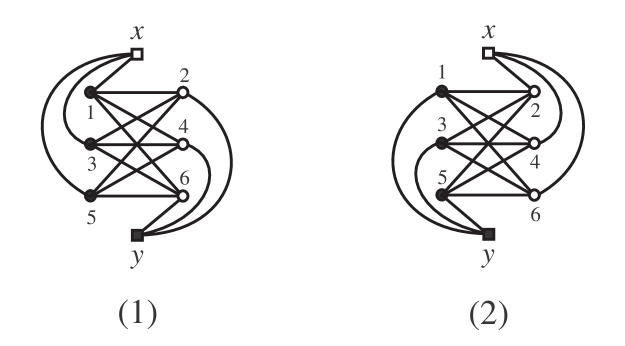
Figure 2.3. (1) $Q_{8}^{(1)}$, (2) $Q_{8}^{(2)}$

Lemma 2-6.

For any element $f$ in ${\rm SE}(K_{3,3,1,1})$,

$$\sum_{\begin{subarray}{c}{\lambda\in\Gamma_{4,4}^{(2)}(K_{3,3,1,1})}\\ {\rm Type\ C}\end{subarray}}{\rm lk}(f(\lambda))^{2}$$

$$= 2\sum_{\begin{subarray}{c}{\gamma\in\Gamma_{8}(K_{3,3,1,1})}\\ {\rm Type\ C}\end{subarray}}a_{2}(f(\gamma))-8\sum_{\gamma\in\Gamma_{6}(K_{3,3})}a_{2}(f(\gamma))$$

$$-2\sum_{\begin{subarray}{c}{\gamma\in\Gamma_{6}(K_{3,3,1,1})}\\ x,y\in\gamma,\ {\rm Type\ C}\end{subarray}}a_{2}(f(\gamma))+2.$$

Proof.

For $k=1,2,\ldots,6$, let us consider subgraphs $F_{x}^{(k)}=(G_{x}-\overline{xk})\cup\overline{xy}\cup\overline{ky}$ and $F_{y}^{(k)}=(G_{y}-\overline{yk})\cup\overline{kx}\cup\overline{yx}$ of $K_{3,3,1,1}$ as illustrated in Fig. 2.4 (1) and (2), respectively. Since each of $F_{x}^{(k)}$ and $F_{y}^{(k)}$ is also homeomorphic to $P_{7}$, by applying Theorem 2-2 (2) to $f|_{F_{x}^{(k)}}$, it follows that

$$\sum_{\begin{subarray}{c}{\lambda=\gamma\cup\gamma^{\prime}\in\Gamma_{4,4}^{(2)}(F_{x}^{(ij)})}\\ x,y\in\gamma,\ {\rm Type\ C}\end{subarray}}{\rm lk}(f(\lambda))^{2}+\sum_{\begin{subarray}{c}{\lambda\in\Gamma_{3,4}^{(2)}(G_{x})}\\ \overline{xk}\not\subset\lambda\end{subarray}}{\rm lk}(f(\lambda))^{2}$$

$$= 2\left\{\sum_{\gamma\in\Gamma_{8}(F_{x}^{(k)})}a_{2}(f(\gamma))+\sum_{\begin{subarray}{c}{\gamma\in\Gamma_{7}(G_{x})}\\ \overline{xk}\not\subset\gamma\end{subarray}}a_{2}(f(\gamma))\right\}-4\sum_{\gamma\in\Gamma_{6}(K_{3,3})}a_{2}(f(\gamma))$$

$$-2\left\{\sum_{\begin{subarray}{c}{\gamma\in\Gamma_{6}(F_{x}^{(k)})}\\ x,y\in\gamma\end{subarray}}a_{2}(f(\gamma))+\sum_{\begin{subarray}{c}{\gamma\in\Gamma_{5}(G_{x})}\\ \overline{xk}\not\subset\gamma\end{subarray}}a_{2}(f(\gamma))\right\}+1.$$

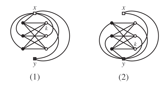
Figure 2.4. (1) $F_{x}^{(k)}$, (2) $F_{y}^{(k)}$ $(k=1,2,3,4,5,6)$

Let us take the sum of both sides of (2) over $k=1,2,\ldots,6$. For an element $\gamma$ in $\Gamma_{8}(K_{3,3,1,1})$, if $\gamma$ is of Type C, then there uniquely exists $F_{x}^{(k)}$ containing $\gamma$. This implies that

(2.22) $$\sum_{k}\left(\sum_{\gamma\in\Gamma_{8}(F_{x}^{(k)})}a_{2}(f(\gamma))\right)=\sum_{\begin{subarray}{c}{\gamma\in\Gamma_{8}(K_{3,3,1,1})}\\ {\rm Type\ C}\end{subarray}}a_{2}(f(\gamma)).$$

For an element $\gamma$ of $\Gamma_{7}(G_{x})$, there exist exactly four edges which are incident to $x$ such that they are not contained in $\gamma$. Thus $\gamma$ is common for exactly four $F_{x}^{(k)}$’s. This implies that

(2.23) $$\sum_{k}\left(\sum_{\begin{subarray}{c}{\gamma\in\Gamma_{7}(G_{x})}\\ \overline{xk}\not\subset\gamma\end{subarray}}a_{2}(f(\gamma)).\right)=4\sum_{\Gamma_{7}(G_{x})}a_{2}(f(\gamma)).$$

It is clear that any element $\gamma$ in $\Gamma_{6}(K_{3,3})$ is common for exactly six $F_{x}^{(k)}$’s. This implies that

(2.24) $$\sum_{k}\left(\sum_{\gamma\in\Gamma_{6}(K_{3,3})}a_{2}(f(\gamma))\right)=6\sum_{\gamma\in\Gamma_{6}(K_{3,3})}a_{2}(f(\gamma)).$$

For an element $\gamma$ in $\Gamma_{6}(K_{3,3,1,1})$ containing $x$ and $y$, if $\gamma$ is of Type C, then there uniquely exists $F_{x}^{(k)}$ containing $\gamma$. This implies that

(2.25) $$\sum_{k}\left(\sum_{\begin{subarray}{c}{\gamma\in\Gamma_{6}(F_{x}^{(k)})}\\ x,y\in\gamma\end{subarray}}a_{2}(f(\gamma))\right)=\sum_{\begin{subarray}{c}{\gamma\in\Gamma_{6}(K_{3,3,1,1})}\\ x,y\in\gamma,\ {\rm Type\ C}\end{subarray}}a_{2}(f(\gamma)).$$

For an element $\gamma$ of $\Gamma_{5}(G_{x})$, there exist exactly four edges which are incident to $x$ such that they are not contained in $\gamma$. Thus $\gamma$ is common for exactly four $F_{x}^{(k)}$’s. This implies that

(2.26) $$\sum_{k}\left(\sum_{\begin{subarray}{c}{\gamma\in\Gamma_{5}(G_{x})}\\ \overline{xk}\not\subset\gamma\end{subarray}}a_{2}(f(\gamma))\right)=4\sum_{\gamma\in\Gamma_{5}(G_{x})}a_{2}(f(\gamma)).$$

For an element $\lambda=\gamma\cup\gamma^{\prime}$ in $\Gamma_{4,4}^{(2)}(K_{3,3,1,1})$, if $\lambda$ is of Type C, then there uniquely exists $F_{x}^{(k)}$ containing $\lambda$. This implies that

(2.27) $$\sum_{k}\left(\sum_{\begin{subarray}{c}{\lambda=\gamma\cup\gamma^{\prime}\in\Gamma_{4,4}^{(2)}(F_{x}^{(k)})}\\ x,y\in\gamma,\ {\rm TypeC}\end{subarray}}{\rm lk}(f(\lambda))^{2}\right)=\sum_{\begin{subarray}{c}{\lambda\in\Gamma_{4,4}^{(2)}(K_{3,3,1,1})}\\ {\rm Type\ C}\end{subarray}}{\rm lk}(f(\lambda))^{2}.$$

For an element $\lambda$ in $\Gamma_{3,4}^{(2)}(G_{x})$, there exist exactly four edges which are incident to $x$ such that they are not contained in $\lambda$. Thus $\lambda$ is common for exactly four $F_{x}^{(k)}$’s. This implies that

(2.28) $$\sum_{k}\left(\sum_{\begin{subarray}{c}{\lambda\in\Gamma_{3,4}^{(2)}(G_{x})}\\ \overline{xk}\not\subset\lambda\end{subarray}}{\rm lk}(f(\lambda))^{2}\right)=4\sum_{\lambda\in\Gamma_{3,4}^{(2)}(G_{x})}{\rm lk}(f(\lambda))^{2}.$$

Then by (2), (2.22), (2.23), (2.24), (2.25), (2.26), (2.27) and (2.28), we have

$$\sum_{\begin{subarray}{c}{\lambda\in\Gamma_{4,4}^{(2)}(K_{3,3,1,1})}\\ {\rm Type\ C}\end{subarray}}{\rm lk}(f(\lambda))^{2}+4\sum_{\lambda\in\Gamma_{3,4}^{(2)}(G_{x})}{\rm lk}(f(\lambda))^{2}$$

$$= 2\sum_{\begin{subarray}{c}{\gamma\in\Gamma_{8}(K_{3,3,1,1})}\\ {\rm Type\ C}\end{subarray}}a_{2}(f(\gamma))+8\sum_{\gamma\in\Gamma_{7}(G_{x})}a_{2}(f(\gamma))-24\sum_{\gamma\in\Gamma_{6}(K_{3,3})}a_{2}(f(\gamma))$$

$$-2\sum_{\begin{subarray}{c}{\gamma\in\Gamma_{6}(K_{3,3,1,1})}\\ x,y\in\gamma,\ {\rm Type\ C}\end{subarray}}a_{2}(f(\gamma))-8\sum_{\gamma\in\Gamma_{5}(G_{x})}a_{2}(f(\gamma))+6.$$

Then by combining (2) and (2), we have the reslut. We remark here that by by applying Theorem 2-2 (2) to $f|_{F_{y}^{(k)}}$ combining the same argument as in the case of $F_{x}^{(k)}$ with (2), we also have (2-6). ∎

Proof of Theorem 1-4..

(1) Let $f$ be an element in ${\rm SE}(K_{3,3,1,1})$. Then by combining (2-4), (2-5) and (2-6), we have

$$\sum_{\lambda\in\Gamma_{3,5}^{(2)}(K_{3,3,1,1})}{\rm lk}(f(\lambda))^{2}+2\sum_{\lambda\in\Gamma_{4,4}^{(2)}(K_{3,3,1,1})}{\rm lk}(f(\lambda))^{2}$$

$$= 4\sum_{\gamma\in\Gamma_{8}(K_{3,3,1,1})}a_{2}(f(\gamma))-4\left\{\sum_{\gamma\in\Gamma_{7}(G_{x})}a_{2}(f(\gamma))+\sum_{\gamma\in\Gamma_{7}(G_{y})}a_{2}(f(\gamma))\right\}$$

$$-4\left\{\sum_{\begin{subarray}{c}{\gamma\in\Gamma_{6}(G_{x})}\\ x\in\gamma\end{subarray}}a_{2}(f(\gamma))+\sum_{\begin{subarray}{c}{\gamma\in\Gamma_{6}(G_{y})}\\ y\in\gamma\end{subarray}}a_{2}(f(\gamma))+\sum_{\begin{subarray}{c}{\gamma\in\Gamma_{6}(K_{3,3,1,1})}\\ x,y\in\gamma\\ {\rm Type\ A,B,C}\end{subarray}}a_{2}(f(\gamma))\right\}$$

$$-4\left\{\sum_{\gamma\in\Gamma_{5}(G_{x})}a_{2}(f(\gamma))+\sum_{\gamma\in\Gamma_{5}(G_{y})}a_{2}(f(\gamma))\right\}+18.$$

Note that

$$\Gamma_{k}(G_{x})\cup\Gamma_{k}(G_{y})=\left\{\gamma\in\Gamma_{k}(K_{3,3,1,1})\ |\ \left\{x,y\right\}\not\subset\gamma\right\}$$

for $k=5,7$. Moreover, we define a subset $\Gamma_{6}^{\prime}$ of $\Gamma_{6}(K_{3,3,1,1})$ by

$$\Gamma_{6}^{\prime} = \left\{\gamma\in\Gamma_{6}(G_{x})\ |\ x\in\gamma\right\}\cup\left\{\gamma\in\Gamma_{6}(G_{y})\ |\ y\in\gamma\right\}$$

$$\cup\left\{\gamma\in\Gamma_{6}(K_{3,3,1,1})\ |\ x,y\in\gamma,\ \gamma{\rm\ is\ of\ Type\ A,B\ or\ C}\right\}.$$

Then we see that (2) implies (1).

(2) Let $f$ be an element in ${\rm SE}(K_{3,3,1,1})$. Let us consider subgraphs $H_{1}=Q_{8}^{(1)}\cup\overline{xy}$ and $H_{2}=Q_{8}^{(2)}\cup\overline{xy}$ of $K_{3,3,1,1}$ as illustrated in Fig. 2.5 (1) and (2), respectively. For $i=1,2$, $H_{i}$ has the proper minor $H^{\prime}_{i}=H_{i}/\overline{xy}$ which is isomorphic to $P_{7}$. For a spatial embedding $f|_{H_{i}}$ of $H_{i}$, there exists a spatial embedding $f^{\prime}$ of $H^{\prime}_{i}$ such that $f^{\prime}(H^{\prime}_{i})$ is obtained from $f(H_{i})$ by contracting $f(\overline{xy})$ into one point. Note that this embedding is unique up to ambient isotopy in ${\mathbb{R}}^{3}$. Then by Corollary 2-3, there exists an element $\mu^{\prime}_{i}$ in $\Gamma_{3,4}^{(2)}(H^{\prime}_{i})$ such that ${\rm lk}(f^{\prime}(\mu^{\prime}_{i}))\equiv 1\pmod{2}\ (i=1,2)$. Note that $\mu^{\prime}_{i}$ is mapped onto an element $\mu_{i}$ in $\Gamma_{4,4}(H_{i})$ by the natural injection from $\Gamma_{3,4}(H^{\prime}_{i})$ to $\Gamma_{4,4}(H_{i})$. Since $f^{\prime}(\mu^{\prime}_{i})$ is ambient isotopic to $f(\mu_{i})$, we have ${\rm lk}(f(\mu_{i}))\equiv 1\pmod{2}\ (i=1,2)$. We also note that both $\mu_{1}$ and $\mu_{2}$ are of Type C in $\Gamma_{4,4}^{(2)}(K_{3,3,1,1})$.

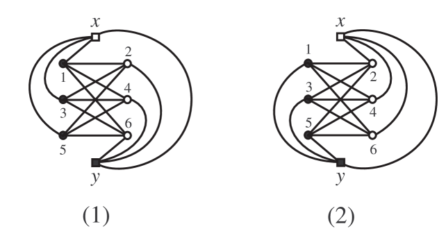
Figure 2.5. (1) $H_{1}$, (2) $H_{2}$

For $v=x,y$ and $i,j,k=1,2,\ldots,6\ (i\neq j)$, let $P_{8}^{(k)}(v;ij)$ be the subgraph of $K_{3,3,1,1}$ as illustrated in Fig. 2.6 (1) if $v=y$, $k\in\left\{1,3,5\right\}$ and $i,j\in\left\{2,4,6\right\}$, (2) if $v=y$, $k\in\left\{2,4,6\right\}$ and $i,j\in\left\{1,3,5\right\}$, (3) if $v=x$, $k\in\left\{1,3,5\right\}$ and $i,j\in\left\{2,4,6\right\}$ and (4) if $v=x$, $k\in\left\{2,4,6\right\}$ and $i,j\in\left\{1,3,5\right\}$. Note that there exist exactly thirty six $P_{8}^{(k)}(v;ij)$’s and they are isomorphic to $P_{8}$ in the $K_{6}$-family. Thus by Corollary 2-3, there exists an element $\lambda$ in $\Gamma^{(2)}(P_{8}^{(k)}(v;ij))$ such that ${\rm lk}(f(\lambda))\equiv 1\pmod{2}$. All elements in $\Gamma^{(2)}(P_{8}^{(k)}(v;ij))$ consist of exactly four elements in $\Gamma^{(2)}_{3,5}(P_{8}^{(k)}(v;ij))$ and exactly four elements in $\Gamma^{(2)}_{4,4}(P_{8}^{(k)}(v;ij))$ of Type A or Type B because they do not contain the edge $\overline{xy}$. It is not hard to see that any element in $\Gamma_{3,5}^{(2)}(K_{3,3,1,1})$ is common for exactly two $P_{8}^{(k)}(v;ij)$’s, and any element in $\Gamma_{4,4}^{(2)}(K_{3,3,1,1})$ of Type A or Type B is common for exactly four $P_{8}^{(k)}(v;ij)$’s.

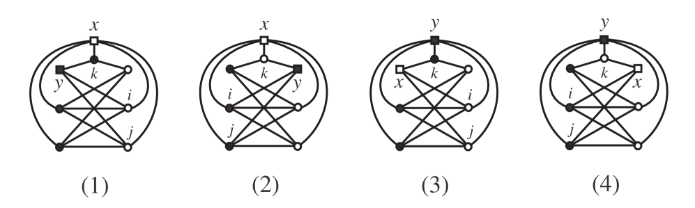
Figure 2.6. $P_{8}^{(k)}(v;ij)$

By (2-4), there exist a nonnegative integer $m$ such that

$$\sum_{\lambda\in\Gamma_{3,5}^{(2)}(K_{3,3,1,1})}{\rm lk}(f(\lambda))^{2}=2m.$$

If $2m\geq 18$, since there exist at least two elements $\mu_{1}$ and $\mu_{2}$ in $\Gamma_{4,4}^{(2)}(K_{3,3,1,1})$ of Type C such that ${\rm lk}(f(\mu_{i}))\equiv 1\pmod{2}\ (i=1,2)$, we have

$$\sum_{\lambda\in\Gamma_{3,5}^{(2)}(K_{3,3,1,1})}{\rm lk}(f(\lambda))^{2}+2\sum_{\lambda\in\Gamma_{4,4}^{(2)}(K_{3,3,1,1})}{\rm lk}(f(\lambda))^{2}\geq 18+4=22.$$

If $2m\leq 16$, then there exist at least $(36-4m)/4=9-m$ elements in $\Gamma_{4,4}^{(2)}(K_{3,3,1,1})$ of Type A or Type B such that each of the corresponding $2$-component links with respect to $f$ has an odd linking number. Then we have

$$\sum_{\lambda\in\Gamma_{3,5}^{(2)}(K_{3,3,1,1})}{\rm lk}(f(\lambda))^{2}+2\sum_{\lambda\in\Gamma_{4,4}^{(2)}(K_{3,3,1,1})}{\rm lk}(f(\lambda))^{2}\geq 2m+2\left\{(9-m)+2\right\}=22.$$

This completes the proof.

∎

3. $\triangle Y$-exchange and Conway-Gordon type formulae

In this section, we give a proof of Theorem 1-8. Let $G_{\triangle}$ and $G_{Y}$ be two graphs such that $G_{Y}$ is obtained from $G_{\triangle}$ by a single $\triangle Y$-exchange. Let $\gamma^{\prime}$ be an element in $\Gamma(G_{\triangle})$ which does not contain $\triangle$. Then there exists an element $\Phi(\gamma^{\prime})$ in $\Gamma(G_{Y})$ such that $\gamma^{\prime}\setminus\triangle=\Phi(\gamma^{\prime})\setminus Y$. It is easy to see that the correspondence from $\gamma^{\prime}$ to $\Phi(\gamma^{\prime})$ defines a surjective map

$$\Phi:\Gamma(G_{\triangle})\setminus\left\{\triangle\right\}\longrightarrow\Gamma(G_{Y}).$$

The inverse image of an element $\gamma$ in $\Gamma(G_{Y})$ by $\Phi$ contains at most two elements in $\Gamma(G_{\triangle})\setminus\Gamma_{\triangle}(G_{\triangle})$. Fig. 3.1 illustrates the case that the inverse image of $\gamma$ by $\Phi$ consists of exactly two elements. Let $\omega$ be a map from $\Gamma(G_{\triangle})$ to ${\mathbb{Z}}$. Then we define the map $\tilde{\omega}$ from $\Gamma(G_{Y})$ to ${\mathbb{Z}}$ by

(3.1) $$\tilde{\omega}(\gamma)=\sum_{\gamma^{\prime}\in\Phi^{-1}(\gamma)}\omega(\gamma^{\prime})$$

for an element $\gamma$ in $\Gamma(G_{Y})$.

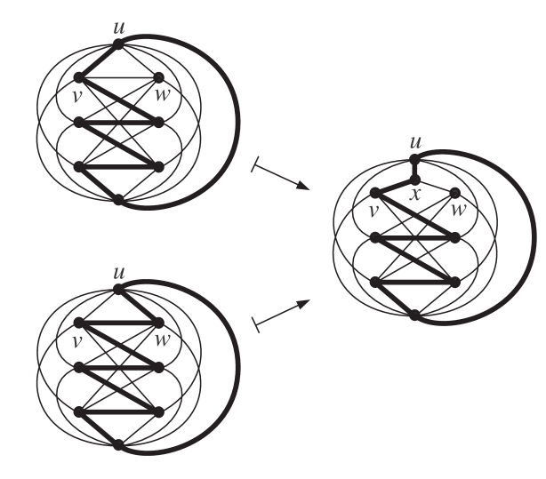
Figure 3.1.

Let $f$ be an element in ${\rm SE}(G_{Y})$ and $D$ a $2$-disk in ${\mathbb{R}}^{3}$ such that $D\cap f(G_{Y})=f(Y)$ and $\partial D\cap f(G_{Y})=\{f(u),f(v),f(w)\}$. Let $\varphi(f)$ be an element in ${\rm SE}(G_{\triangle})$ such that $\varphi(f)(x)=f(x)$ for $x\in G_{\triangle}\setminus\triangle=G_{Y}\setminus Y$ and $\varphi(f)(G_{\triangle})=\left(f(G_{Y})\setminus f(Y)\right)\cup\partial D$. Thus we obtain a map

$$\varphi:{\rm SE}(G_{Y})\longrightarrow{\rm SE}(G_{\triangle}).$$

Then we immediately have the following.

Proposition 3-1.

Let $f$ be an element in ${\rm SE}(G_{Y})$ and $\gamma$ an element in $\Gamma(G_{Y})$. Then, $f(\gamma)$ is ambient isotopic to $\varphi(f)(\gamma^{\prime})$ for each element $\gamma^{\prime}$ in the inverse image of $\gamma$ by $\Phi$.

Then we have the following lemma which plays a key role to prove Theorem 1-8. This lemma has already been shown in [18, Lemma 2.2] in more general form, but we give a proof for the reader’s convenience.

Lemma 3-2.

(Nikkuni-Taniyama [18]) For an element $f$ in ${\rm SE}(G_{Y})$,

$$\sum_{\gamma\in\Gamma(G_{Y})}\tilde{\omega}(\gamma)a_{2}(f(\gamma))=\sum_{\gamma^{\prime}\in\Gamma(G_{\triangle})}\omega(\gamma^{\prime})a_{2}(\varphi(f)(\gamma^{\prime})).$$

Proof.

Since $\varphi(f)(\triangle)$ is the trivial knot, we have

$$\sum_{\gamma^{\prime}\in\Gamma(G_{\triangle})}\omega(\gamma^{\prime})a_{2}(\varphi(f)(\gamma^{\prime}))=\sum_{\gamma^{\prime}\in\Gamma(G_{\triangle})\setminus\left\{\triangle\right\}}\omega(\gamma^{\prime})a_{2}(\varphi(f)(\gamma^{\prime})).$$

Note that

$$\Gamma(G_{\triangle})\setminus\left\{\triangle\right\}=\bigcup_{\gamma\in\Gamma(G_{Y})}\Phi^{-1}(\gamma).$$

Then, by Proposition 3-1, we see that

$$\sum_{\gamma^{\prime}\in\Gamma(G_{\triangle})\setminus\left\{\triangle\right\}}\omega(\gamma^{\prime})a_{2}(\varphi(f)(\gamma^{\prime})) = \sum_{\gamma\in\Gamma(G_{Y})}\left(\sum_{\gamma^{\prime}\in\Phi^{-1}(\gamma)}\omega(\gamma^{\prime})a_{2}(\varphi(f)(\gamma^{\prime}))\right)$$

$$= \sum_{\gamma\in\Gamma(G_{Y})}\left(\sum_{\gamma^{\prime}\in\Phi^{-1}(\gamma)}\omega(\gamma)a_{2}(f(\gamma))\right)$$

$$= \sum_{\gamma\in\Gamma(G_{Y})}\tilde{\omega}(\gamma)a_{2}(f(\gamma)).$$

Thus we have the result. ∎

Proof of Theorem 1-8..

By Corollary 1-5, there exists a map $\omega$ from $\Gamma(K_{3,3,1,1})$ to ${\mathbb{Z}}$ such that for any element $g$ in ${\rm SE}(K_{3,3,1,1})$,

(3.2) $$\sum_{\gamma^{\prime}\in\Gamma(K_{3,3,1,1})}\omega(\gamma^{\prime})a_{2}(g(\gamma^{\prime}))\geq 1.$$

Let $G$ be a graph which is obtained from $K_{3,3,1,1}$ by a single $\triangle Y$-exchange and $\tilde{\omega}$ the map from $\Gamma(G)$ to ${\mathbb{Z}}$ as in (3.1). Let $f$ be an element in ${\rm SE}(G)$. Then by Lemma 3-2 and (3.2), we see that

$$\sum_{\gamma\in\Gamma(G)}\tilde{\omega}(\gamma)a_{2}(f(\gamma))=\sum_{\gamma^{\prime}\in\Gamma(K_{3,3,1,1})}\omega(\gamma^{\prime})a_{2}(\varphi(f)(\gamma^{\prime}))\geq 1.$$

By repeating this argument, we have the result. ∎

Remark 3-3.

In Theorem 1-8, the proof of the existence of a map $\omega$ is constructive. It is also an interesting problem to give $\omega(\gamma)$ for each element $\gamma$ in ${\Gamma}(G)$ concretely.

4. Rectilinear spatial embeddings of $K_{3,3,1,1}$

In this section, we give a proof of Theorem 1-9. For an element $f$ in ${\rm RSE}(G)$ and an element $\gamma$ in $\Gamma_{k}(G)$, the knot $f(\gamma)$ has stick number less than or equal to $k$, where the stick number $s(K)$ of a knot $K$ is the minimum number of edges in a polygon which represents $K$. Then the following is well known.

Proposition 4-1.

(Adams [1], Negami [15]) For any nontrivial knot $K$, it follows that $s(K)\geq 6$. Moreover, $s(K)=6$ if and only if $K$ is a trefoil knot.

We also show a lemma for a rectilinear spatial embedding of $P_{7}$ which is useful in proving Theorem 1-9.

Lemma 4-2.

For an element $f$ in ${\rm RSE}\left(P_{7}\right)$,

$$\sum_{\gamma\in\Gamma_{7}\left(P_{7}\right)}a_{2}(f(\gamma))\geq 0.$$

Proof.

Note that $a_{2}({\rm trivial\ knot})=0$ and $a_{2}({\rm trefoil\ knot})=1$. Thus by Proposition 4-1, $a_{2}(f(\gamma))=0$ for any element $\gamma$ in $\Gamma_{5}(P_{7})$ and $a_{2}(f(\gamma))\geq 0$ for any element $\gamma$ in $\Gamma_{6}(P_{7})$. Moreover, by Corollary 2-3, we have

(4.1) $$\sum_{\lambda\in\Gamma_{3,4}^{(2)}(P_{7})}{\rm lk}(f(\lambda))^{2}\geq 1.$$

Then Theorem 2-2 (2) implies the result. ∎

Proof of Theorem 1-9..

Let $f$ be an element in ${\rm RSE(K_{3,3,1,1})}$. Since $G_{x}$ and $G_{y}$ are isomorphic to $P_{7}$, by Lemma 4-2, we have

(4.2) $$\sum_{\gamma\in\Gamma_{7}\left(G_{x}\right)}a_{2}(f(\gamma))\geq 0,\ \sum_{\gamma\in\Gamma_{7}\left(G_{y}\right)}a_{2}(f(\gamma))\geq 0.$$

Then by Corollary 1-5 and (4.2), we have

$$\sum_{\gamma\in\Gamma_{8}(K_{3,3,1,1})}a_{2}(f(\gamma)) \geq \sum_{\gamma\in\Gamma_{7}\left(G_{x}\right)}a_{2}(f(\gamma))+\sum_{\gamma\in\Gamma_{7}\left(G_{y}\right)}a_{2}(f(\gamma))$$

$$+\sum_{\gamma\in\Gamma_{6}^{\prime}}a_{2}(f(\gamma))+\sum_{\begin{subarray}{c}{\gamma\in\Gamma_{5}(K_{3,3,1,1})}\\ {\left\{x,y\right\}\not\subset\gamma}\end{subarray}}a_{2}(f(\gamma))+1$$

$$\geq 0+0+0+0+1$$

$$= 1.$$

Thus we have the desired conclusion. ∎

Remark 4-3.

All of knots with $s\leq 8$ and $a_{2}>0$ are $3_{1}$, $5_{1}$, $5_{2}$, $6_{3}$, a square knot, a granny knot, $8_{19}$ and $8_{20}$ (Calvo [3]). Therefore, Theorem 1-9 implies that at least one of them appears in the image of every rectilinear spatial embedding of $K_{3,3,1,1}$. On the other hand, it is known that the image of every rectilinear spatial embedding of $K_{7}$ contains a trefoil knot (Brown [2], Ramírez Alfonsín [20], Nikkuni [17]). It is still open whether the image of every rectilinear spatial embedding of $K_{3,3,1,1}$ contains a trefoil knot.

References

[1]
C. C. Adams, The knot book. An elementary introduction to the mathematical theory of knots. Revised reprint of the 1994 original. American Mathematical Society, Providence, RI, 2004.
[2]
A. F. Brown, Embeddings of graphs in , Ph. D. Dissertation, Kent State University, 1977.
[3]
J. A. Calvo,
Geometric knot spaces and polygonal isotopy,
Knots in Hellas ’98, Vol. 2 (Delphi).
J. Knot Theory Ramifications10 (2001), 245–267.
[4]
J. H. Conway and C. McA. Gordon,
Knots and links in spatial graphs,
J. Graph Theory7 (1983), 445–453.
[5]
M. R. Fellows and M. A. Langston,
Non constructive tools for proving polynomial-time decidability,
J. of ACM35 (1988), 727–739.
[6]
E. Flapan and R. Naimi,
The Y-triangle move does not preserve intrinsic knottedness,
Osaka J. Math.45 (2008), 107–111.
[7]
J. Foisy,
Intrinsically knotted graphs,
J. Graph Theory39 (2002), 178–187.
[8]
J. Foisy,
A newly recognized intrinsically knotted graph,
J. Graph Theory43 (2003), 199–209.
[9]
J. Foisy and L. Ludwig,
When graph theory meets knot theory, Communicating mathematics, 67–85,
Contemp. Math.,479, Amer. Math. Soc., Providence, RI, 2009.
[10]
N. Goldberg, T. W. Mattman and R. Naimi,
Many, many more intrinsically knotted graphs,
preprint. (arXiv:math.1109.1632)
[11]
R. Hanaki, R. Nikkuni, K. Taniyama and A. Yamazaki,
On intrinsically knotted or completely -linked graphs,
Pacific J. Math.252 (2011), 407–425.
[12]
H. Hashimoto and R. Nikkuni,
On Conway-Gordon type theorems for graphs in the Petersen family,
J. Knot Theory Ramifications22 (2013), 1350048.
[13]
T. Kohara and S. Suzuki,
Some remarks on knots and links in spatial graphs,
Knots 90 (Osaka, 1990), 435–445, de Gruyter, Berlin, 1992.
[14]
R. Motwani, A. Raghunathan and H. Saran,
Constructive results from graph minors: Linkless embeddings,
29th Annual Symposium on Foundations of Computer Science, IEEE, 1988, 398–409.
[15]
S. Negami,
Ramsey theorems for knots, links and spatial graphs,
Trans. Amer. Math. Soc.324 (1991), 527–541.
[16]
J. Nešetřil and R. Thomas,
A note on spatial representation of graphs,
Comment. Math. Univ. Carolinae26 (1985), 655–659.
[17]
R. Nikkuni,
A refinement of the Conway-Gordon theorems,
Topology Appl.156 (2009), 2782–2794.
[18]
R. Nikkuni and K. Taniyama,
-exchanges and the Conway-Gordon theorems, J. Knot Theory Ramifications21 (2012), 1250067.
[19]
D. O’Donnol,
Knotting and linking in the Petersen family, preprint. (arXiv:math.1008.0377 )
[20]
J. L. Ramírez Alfonsín,
Spatial graphs and oriented matroids: the trefoil,
Discrete Comput. Geom.22 (1999), 149–158.
[21]
N. Robertson and P. Seymour,
Graph minors. XX. Wagner’s conjecture,
J. Combin. Theory Ser. B92 (2004), 325–357.
[22]
N. Robertson, P. Seymour and R. Thomas,
Sachs’ linkless embedding conjecture,
J. Combin. Theory Ser. B64 (1995), 185–227.
[23]
H. Sachs,
On spatial representations of finite graphs,
Finite and infinite sets, Vol. I, II (Eger, 1981), 649–662,
Colloq. Math. Soc. Janos Bolyai, 37, North-Holland, Amsterdam, 1984.
[24]
K. Taniyama and A. Yasuhara,
Realization of knots and links in a spatial graph,
Topology Appl.112 (2001), 87–109.