A local bias approach to the clustering of discrete density peaks
Abstract
Maxima of the linear density field form a point process that can be used to understand the spatial distribution of virialized halos that collapsed from initially overdense regions. However, owing to the peak constraint, clustering statistics of discrete density peaks are difficult to evaluate. For this reason, local bias schemes have received considerably more attention in the literature thus far. In this paper, we show that the 2-point correlation function of maxima of a homogeneous and isotropic Gaussian random field can be thought of, up to second order at least, as arising from a local bias expansion formulated in terms of rotationally invariant variables. This expansion relies on a unique smoothing scale, which is the Lagrangian radius of dark matter halos. The great advantage of this local bias approach is that it circumvents the difficult computation of joint probability distributions. We demonstrate that the bias factors associated with these rotational invariants can be computed using a peak-background split argument, in which the background perturbation shifts the corresponding probability distribution functions. Consequently, the bias factors are orthogonal polynomials averaged over those spatial locations that satisfy the peak constraint. In particular, asphericity in the peak profile contributes to the clustering at quadratic and higher order, with bias factors given by generalized Laguerre polynomials. We speculate that our approach remains valid at all orders, and that it can be extended to describe clustering statistics of any point process of a Gaussian random field. Our results will be very useful to model the clustering of discrete tracers with more realistic collapse prescriptions involving the tidal shear for instance.
pacs:
98.80.-k, 98.65.-r, 95.35.+d, 98.80.EsI Introduction
In the biasing scenario introduced by 1984ApJ…284L…9K , virialized halos form out of initially overdense regions with a linear density (extrapolated to the redshift of interest) equal to . Since then, this picture has received considerable support from observational data. Even though dark matter halos are extended objects, they form a spatial point process as far as their clustering is concerned. However, this essential feature has remained elusive in most theoretical descriptions of halo clustering, which assume that halos are a Poisson sampling of a more fundamental, continuous halo density field .
The peak formalism first proposed by 1985MNRAS.217..805P ; 1986ApJ…304…15B in a cosmological context is interesting because it is a well-behaved point process. In this approach, virialized halos are associated with maxima of the initial density field. The displacement from their initial (Lagrangian) to final (Eulerian) position can be computed upon assuming phase space conservation 2010PhRvD..82j3529D . Clustering statistics of these discrete density peaks display many of the features present in measurements of halo clustering extracted from N-body simulations. In particular, discrete density peaks exhibit a -dependent linear bias factor 1999ApJ…525..543M ; 2008PhRvD..78j3503D , small-scale exclusion 1989MNRAS.238..293L ; 1989MNRAS.238..319C , and a linear velocity bias 2010PhRvD..81b3526D etc. Some of these predictions have recently been tested in numerical simulations 2011MNRAS.413.1961L ; 2012MNRAS.421.3472E : peaks of the linear density field appear to provide a good approximation to the formation sites of dark matter halos with .
However, despite recent progress towards the computation of peak clustering statistics 2010PhRvD..82j3529D and a formulation of peak theory within the excursion set formalism 2012MNRAS.426.2789P ; 2012arXiv1210.1483P , discrete density peaks lack a clear connection with the more conventional local bias schemes 1993ApJ…413..447F , in which halos are approximated as a continuous field. Furthermore, while in the local bias model the computation of halo correlation functions is straightforward (though there are ambiguities regarding the filtering scale etc.), in the peak formalism calculations are particularly tedious owing to the peak constraint 1986ApJ…304…15B ; 1995MNRAS.272..447R ; 2008PhRvD..78j3503D ; 2010PhRvD..82j3529D . In the most comprehensive analysis thus far, ref. 2010PhRvD..82j3529D succeeded in computing the peak 2-point correlation up to second order, including the Zel’dovich displacement. They showed that some of the first- and second-order contributions could be obtained from a peak-background split formulated in terms of conditional mass functions. In contrast to most analytic models of halo clustering, which assume that the (-independent) bias coefficients are the peak-background split biases, they derived this equivalence from first principles. However, they could not determine the physical origin of the other second-order contributions. Moreover, the peak constraint is clearly too simplistic to describe the clustering of low mass halos. In this mass range, one should consider more elaborated constraints involving the tidal shear etc. In this regards, it would be very desirable to find a simpler way of computing the correlation functions of generic point processes of a (Gaussian) random field.
In this paper, we suggest a simple, physically motivated prescription based on the peak-background split to compute the correlation functions of generic point processes driven by homogeneous and isotropic Gaussian random fields. We argue that clustering statistics of such point processes can be reduced to the evaluation of correlators of an effective continuous overdensity which, in the case of discrete peaks, is a function of the local (smoothed) mass density field and its derivatives. Our approach combines in a single coherent picture peak theory, peak-background split, local bias and the excursion set framework. For sake of clarity, we will focus on the 2-point correlation function of initial density peaks as computed in 2010PhRvD..82j3529D to explain the fundamentals of our approach.
The paper is organized as follows. Sec. II furnishes a brief summary of clustering in peak theory. Sec. III is the central Section of the paper, where we present the connection between rotational invariants, peak-background split and a local peak bias prescription. Finally, Sec.IV discusses the implications of our findings.
II Correlation functions for density peaks
We begin with a short recapitulation of the computation of correlation functions in the peak formalism. Let be the linear mass density field smoothed on scale with a spherically symmetric filter. For convenience, we work with the normalized variables , and . Here, is the peak height or significance, and
| (1) |
are moments of the power spectrum . A Gaussian filter is frequently adopted to ensure convergence of all the spectral moments , but one should bear in mind that the peak height associated with dark matter halos is always computed with a tophat filter (see 2012arXiv1210.1483P for details). The first few spectral moments can be combined into a dimensionless spectral width that takes values between zero and unity. reflects the range over which the smoothed power spectrum is significant, i.e. for a sharply peaked power spectrum whereas for a power spectrum that covers a wide range of wavenumbers.
Correlations of density maxima of can be evaluated using the Kac-Rice formula (Kac1943, ; Rice1945, ). The trick is to Taylor-expand around the position of a local maximum. As a result, the number density of (BBKS) peaks of height at position in the smoothed density field can be expressed in terms of the field and its derivatives:
| (2) | ||||
where is the characteristic radius of a peak (and not the interpeak distance). The three-dimensional Dirac distribution ensures that all extrema are included. The factors of theta function , where is the lowest eigenvalue of the shear tensor , and the Dirac delta further restricts the set to density maxima of the desired significance .
The (disconnected) -point correlations (or joint intensities) of density maxima are defined as the ensemble averages of products of ,
| (3) |
For the Gaussian initial conditions considered here, multivariate normal distribution are assumed to perform the ensemble average. In the particular case , is the average, differential number density of peaks of height identified on the filtering scale (1986ApJ…304…15B, ),
| (4) | ||||
In the last equality, is the typical 3-dimensional extent of a density peak 2012MNRAS.426.2789P . The functions are defined in Appendix B. In particular, the ratio is equal to the th moment of the peak curvature . Similarly, the reduced 2-point correlation function for maxima of a given significance separated by a distance is
| (5) |
Notice that, in , we have ignored the shot-noise term that arises from the self-pairs as it matters only at zero-lag (in the peak power spectrum however, this contributes a constant Poisson noise at all wavenumbers).
The calculation of Eq.(5) at second order in the mass correlation and its derivatives is quite tedious 1986ApJ…304…15B ; 1995MNRAS.272..447R ; 2010PhRvD..82j3529D because one must evaluate the joint probability distribution for the 10-dimensional vector of variables at two different spatial locations and , i.e. a total of 20 variables. Here, the components symbolize the independent entries of . Fortunately, as was shown in 2010PhRvD..82j3529D , most of the terms nicely combine together, so that the final result can be recast into the compact expression
| (6) |
The functions are quantities analogous to but defined for a finite separation ,
| (7) |
where are spherical Bessel functions. In the right-hand side of Eq.(II), all the correlations depend on the filtering scale and the separation. However, the first line contains terms involving the first and second order peak bias parameters and (to be defined shortly), the second line retains a -dependence through the function solely, whereas the last two terms in the right-hand side depend on the separation (and ) only. Hence, unlike standard local bias expansions (Eulerian or Lagrangian), the peak 2-point correlation also exhibits quadratic terms linear in the second-order bias . These terms involve derivatives of the linear mass correlation and, therefore, vanish at zero lag. Clearly, they arise because the peak correlation also depends on the statistical properties of and .
Ref. 2010PhRvD..82j3529D also showed that the Lagrangian peak bias factors can be constructed upon averaging over the peak curvature products of and , where
| (8) | ||||
| (9) |
For peak of significance on the smooting scale , the first order bias is defined as the Fourier space multiplication (we omit the dependence on and for shorthand convenience) 2008PhRvD..78j3503D
| (10) | |||
The overline designates the average over the peak curvature. can be quite large for moderate peak heights. In the high peak limit however, it is negligible so that is nearly scale-independent (like in local bias models). Similarly, the Fourier space expression of the second order peak bias is 2010PhRvD..82j3529D
| (11) |
where and are wavemodes and the -independent coefficients , and are
| (12) | ||||
| (13) | ||||
and
| (14) | ||||
By definition, acts on the functions and as follows:
| (15) |
As pointed out by 2010PhRvD..82j3529D , the piece can be thought of as arising from the continuous, deterministic, local bias relation
| (16) | ||||
where the bias factors are peak-background split bias factors that follow from expanding the conditional peak number density in a series in the small background density perturbation . This expansion is local in the sense that, except for the filtering, it involves quantities evaluated at solely. However, an essential difference with the widespread local bias model 1993ApJ…413..447F is the fact that, when computing the ensemble average , we must ignore all powers of zero-lag moments (such as, e.g., in ) to recover since the latter does not exhibit such contributions (this ’no zero-lag requirement’ also arises in the derivation of the ’renormalized’ bias parameters of 2012arXiv1212.0868S ). All the terms in Eq.(16) are of course invariant under rotations since transforms as a scalar under rotations. Clearly however, this series expansion is not the most generic Lagrangian expansion we may conceive of (see, e.g., 2012arXiv1207.7117S non nonlocal Lagrangian bias).
Notwithstanding these results, 2010PhRvD..82j3529D did not succeed in finding a physical interpretation of the other second-order terms in the right-hand side of Eq.(II), even though it was pretty clear that they – at least partially – arise from coupling involving the components of the gradient and the hessian .
III A intuitive interpretation of
In this Section, we propose an intuitive, physically motivated explanation of Eq. (II) that is grounded in the peak-background split argument 1984ApJ…284L…9K . We begin with a brief introduction to the helicity basis, which was used in 2010PhRvD..82j3529D to compute probability distributions of the density field and its derivatives at two different spatial locations.
III.1 Probability density in the helicity basis
The 2-point correlation function of initial density peaks is the ensemble average of over the joint probability density , where are the values of the field and its derivatives at position . In what follows, will also designate Eq.(2). Following 2010PhRvD..82j3529D , we can decompose the variables that appear in the joint probability density in the helicity basis , where
| (17) |
and , , and are orthonormal vectors in spherical coordinates . The orthogonality relations between these vectors are and , where the inner product between two vectors and is defined as . Unless otherwise stated, an overline will denote complex conjugation throughout Sec. III.1.
In this reference frame, we decompose the first derivatives as
| (18) |
Here, and are the helicity-0 and -1 components. The correlation properties of and can be obtained by projecting out the scalar and vector parts of the correlation of the Cartesian components with the projection operator . The rule of thumb is that , where , vanish unless . We find
| (19) | ||||
Here and henceforth, the subscripts “1” and “2” will denote variables evaluated at position and for shorthand convenience. Similarly, the symmetric tensor can be decomposed into its trace and traceless components,
| (20) | ||||
The variables and are the longitudinal and transverse helicity-0 modes, are the components of a transverse vector, , whereas is a symmetric, traceless, transverse tensor, . Explicit expressions for these variables are
| (21) | ||||
| (22) | ||||
| (23) | ||||
where , and are the scalar, vector and tensor projections operators (see, e.g., 1994FCPh…15..209D ). We have introduced factors of and in the decomposition Eq.(20) such that the zero-point moments of the helicity-0, -1 and -2 variables all equal (see Eq. (24) below). The helicity-1 components of and their complex conjugates are given by and , whereas and are the two independent helicity-2 modes (polarizations) and their complex conjugates, respectively. Hereafter designating as , the correlation properties of these variables are the following:
| (24) | ||||
and . All the other correlations vanish. Note that the covariances are real despite the fact that the helicity-1 and -2 variables are complex.
While the average peak number density only depends on the matrix of covariances at the same location, the computation of the peak 2-point correlation function and higher-order clustering statistics from Eq. (3) generally involve covariances of the random fields at different locations. For , the covariance matrix , where , is a 20-dimensional matrix that may be partitioned into four block matrices: the zero-point contribution in the top left and bottom right corners, and the cross-correlation matrix and its transpose in the bottom left and top right corners, respectively. Expressions for and in the helicity basis can be found in the Appendix of 2010PhRvD..82j3529D .
III.2 Rotational invariants
Translational and rotational invariance implies that does not depend on spatial position, and that be a function of the distance solely. In this regards, 2010PhRvD..82j3529D noted that, although the covariance matrix in the helicity basis (17) does not depend on the direction of the separation vector , it is not equal to the angular average covariance matrix . The latter is obtained upon setting whenever in the expression of . As a consequence, retains the correlations , , and parts of the covariances and . However, 2010PhRvD..82j3529D did not provide a convincing explanation for their observation. We shall do it now.
Firstly, it is pretty clear that, since the peak 2-point correlation is invariant under rotations of the reference frame, it should be possible to express it in terms of rotational invariants constructed from the variables , and . The peak significance and the trace are two obvious candidates, but they are not the only ones. The vector of first derivatives and the traceless matrix yield two additional invariants, i.e. the square modulus and the trace . In the helicity basis, these invariants can be written
| (25) |
and
| (26) |
The symmetric matrix actually provides a third invariant with respect to rotations: the determinant det. However, as we shall see below in the discussion of the peak-background split, because this determinant only enters the peak number density and not the 1-point multivariate normal distribution (the argument of the exponential is quadratic in the variables), it does not contribute directly to the peak bias. This suggests that we look at the covariances of and , where these are defined as
| (27) | ||||
| (28) |
where are the Fourier modes of the smoothed density field. As we shall see in Sec. III.3, the variables and are distributed as chi-squared () variates with 3 and 5 degrees of freedom, respectively. Using either the Fourier space expression of (not to be confonded here with a cartesian component of the vector ) or the fact that only components of identical helicity correlate, it is straightforward to compute the following correlators (for illustrative purposes, Appendix A furnishes details of the calculation of ):
| (29) | ||||
| (30) |
Ignoring the zero-lag contributions, these terms correspond exactly (up to a sign factor) to some of those entering the second-order contribution of in Eq.(II), with being proportional to in particular. The computations of correlators involving proceeds in a similar way although, in this case, it is much easier to sum the correlations among equal helicity components. For instance,
| (31) | ||||
where we used the fact that . After some algebra, we find
| (32) |
and
| (33) | ||||
| (34) |
The cross-correlations of and with in place of are identical except for the superscript , which should be replaced by . Again, all these terms can be found among the second-order contributions in the right-hand side of Eq. (II).
Therefore, the actual dependence of on the invariants and , whose covariances involve the correlation functions with , is the fundamental reason for being different from the angle average . Those correlations, which arise upon expanding the joint probability density at second order, eventually all nicely combine together (and with terms proportional to and ) to yield the second-order correlators , etc.
The question then arises of the calculation of the coefficients of these quadratic terms in the peak 2-point correlation function. We already know that the coefficients multiplying products of the form are the quadratic peak-background split biases associated to the scalars and . Does this hold also for the coefficients multiplying , etc. ?
III.3 Generalizing the peak background-split
The probability distribution that is needed to compute is a multivariate Gaussian of covariance matrix ,
| (35) |
Owing to rotational invariance, this probability density is a function of , , and solely (see, e.g., 2009PhRvD..80h1301P for a systematic analysis of distribution functions of homogeneous and isotropic random fields). The quadratic form that appears in the exponential factor reads
| (36) |
so that retains factorization with respect to , and . Furthermore, since (with ) and (with ) are complex random variables with mean 0 and variance and respectively and since and at the same spatial location, the quantities and are independent -distributed variables with 3 and 5 degrees of freedom, respectively (similar conclusions can be drawn for the distribution of the components of the deformation tensor, see 2002MNRAS.329…61S ; 2012arXiv1207.7117S ). Therefore, the 1-point probability density can also be written as
| (37) |
where is the bivariate normal
| (38) |
and
| (39) |
is a -distribution with degrees of freedom. Note that the distribution of is coupled with the last rotational invariant 2012PhRvD..85b3011G . However, it can be easily checked that, upon integrating over the (uniform) distribution of , we obtain the -distribution .
Ref. 2010PhRvD..82j3529D discussed how the peak bias factors can be derived from a peak-background split. They argued that, while the -dependent piece is related to the th order derivative of the differential number density , derivatives cannot produce the bias factors , etc. multiplying the -dependent terms. For this reason, they considered a second implementation of the peak-background split 1996MNRAS.282..347M ; 1999MNRAS.308..119S in which the dependence of the mass function on the overdensity of the background is derived explicitly. However, it is possible to write all the peak bias factors as derivatives of rather than . More precisely, the are the bivariate Hermite polynomials
| (40) |
relative to the weight , further averaged over the peak curvature . Therefore, they are peak-background split biases in the sense that they can be derived from the transformation and , where and are long-wavelength background perturbations uncorrelated with the (small-scale) fields and . Ref. 2010PhRvD..82j3529D did not express the peak-background split this way because they considered the effect of a background perturbation after the integration over the peak curvature. In terms of the rotational invariants introduced above, we can write the as
| (41) |
where it is understood that takes the form Eq. (37) and . Factors of and are introduced because bias factors are ordinarily defined relative to the physical field and its derivatives rather than the normalized variables. In practice, the integral is most easily performed upon transforming the 5 degrees of freedom attached to to the shape parameters and and the 3 Euler angles that describe the orientation of the principal axis frame (see Appendix B for details).
In 2012PhRvD..85b3011G , it was noticed that, in the presence of non-Gaussianity, the 1-point probability density can be expanded in the set of orthogonal polynomials associated to the weight provided by in the Gaussian limit. The same logic applies to the peak bias factors. Namely, the are drawn from the orthogonal polynomials associated to , i.e. bivariate Hermite polynomials. Therefore, we expect that and also generate bias parameters, and that these are drawn from the orthogonal polynomials associated with -distributions, i.e. generalized Laguerre polynomials. These are defined as
| (42) |
and are orthogonal over with respect to the -distribution with degrees of freedom. The orthogonality relation can be expressed as
| (43) |
The first generalized Laguerre polynomials are and .
Given the correlator Eq. (29), the term proportional to in the right-hand side of Eq.(II) indicates that the first-order bias parameter associated with the invariant is . The aforementioned considerations suggest that we define the th-order bias factor as the Laguerre polynomial averaged over all the possible peak configurations, i.e.
| (44) |
Taking into account the peak constraint, the first-order bias factors thus is
| (45) | ||||
| (46) |
which is precisely what we were expecting. Similarly, we define the bias parameter associated to the invariant as the ensemble average of the Laguerre polynomial orthogonal with respect to the weight . Namely,
| (47) |
Note that, although we use a single symbol to designate the bias factors derived from the -distributions, the variables and , unlike and , are uncorrelated. The first-order bias factor thus is
| (48) |
To evaluate the integral, we first express the measure in terms of the ellipticity and prolateness , so that can be written as (see Appendix B for details). A multiplicative factor of will arise upon, e.g., taking the derivative of with respect to . In the notation of 2010PhRvD..82j3529D , our factor of precisely corresponds to their derivative term evaluated at (see Appendix B). Taking into account the factor of in the denominator, can eventually be written
| (49) |
The physical interpretation of this result is straightforward: is a scalar that describes the asymmetry of the peak density profile. In the high peak limit, reflecting the fact that the most prominent peaks are nearly spherical (see Fig.9 of 2010PhRvD..82j3529D ).
The physical origin for the appearance of these orthogonal polynomials can be found in the peak-background split. Long-wavelength background perturbations locally modulate the mean of the distributions , and . The resulting non-central distributions can then be expanded in the appropriate set of orthogonal polynomials. In practice, it is convenient to introduce a shift or translation operator to describe the action of a background perturbation on the distribution of rotational invariants. For the scalars and , we define the shift operator as
| (50) |
where and are small perturbations to the peak significance and the peak curvature, i.e. and . The action of on the probability density is to shift the (zero) mean of and by and , respectively (the reason for the minus sign is that Hermite polynomials include a factor of ). A straightforward calculation gives
| (51) | ||||
where and are given in Eqs.(8) and (9), and is the exponential factor in with the replacement and . The last expression is a generating function of bivariate Hermite polynomials. On expanding it in the small parameters and ,
| (52) |
we recover the bias factors once the results are averaged over all locations that satisfy the peak constraint. Note that the bias parameter defined in 2012arXiv1212.0868S bears the same physical meaning as our : both represent the leading-order response of the tracer abundance to a uniform shift in the curvature of the density field.
For the quadratic variables and , Eq.(42) suggests that we express the shift operator in terms of both and . The definition is somewhat cumbersome because we must take into account not only the ordering of and , but also the factor of in the orthogonality relation Eq.(43). A sensible definition of for the variable and is
| (53) | ||||
| (54) |
where is a modified Bessel function of the first kind and the symbol of normal ordering is borrowed from quantum field theory. In the present discussion, the normal ordering is defined as
| (55) |
where is some test function. With this definition, the action of on a -distribution with degrees of freedom is
| (56) | ||||
This is precisely the Laguerre series expansion of a non-central -variate derived in tiku:1965 (see Appendix C). Therefore,
where is a non-central -distribution with degrees of freedom and non-centrality parameter . The latter is defined as the sum of squares , where are the means of the random variables. We can now read off the bias factors from the expansion of in generalized Laguerre polynomials. For instance,
| (57) |
Note that the more common generating function
| (58) |
appears to bear little connection with the non-central -distribution.
To better understand the reason why the peak-background split generates a non-central -distribution, we note that, owing to the relation between Hermite and Laguerre polynomials, we could also have defined and as second derivatives of , where is now the vector of independent normal random variables such that and . A little algebra shows that
| (59) |
Another way of writing this formula would be to absorb a factor of in the definition of (and thus explicitly deal with complex normal distributions). Analogously, we have
| (60) |
This suggests that the effect of a background perturbation on and can also be thought of as shifting the components of the first derivatives according to , and those of according to . The small perturbations and need not be the same for distinct and/or . However, owing to invariance under rotations, only the length of the vector and matter. This is the reason why the background perturbation effectively shifts the respective -distributions to non-central -distributions, with non-centrality parameter and . Note that it should be possible to formulate this peak-background split with the conditional peak number density in a large-scale region of overdensity , like in 2010PhRvD..82j3529D . However, one should then consider two long-wavelength perturbations and in order to describe the effect of the background perturbation on and , in addition to (which suffices to describe the effect of the background wave for both and since these variables are correlated).
To conclude, 2011PhRvD..83h3518M also pointed out that, even though there is no functional relation for discrete density peaks, it is nevertheless possible to define renormalized bias parameters as the expectation values . However, he did not compute them explicitly, nor specified what is (though it is pretty clear that it is related to ). Here, we demonstrated explicitly that each of the combinations , and of rotational invariants generates a set of orthogonal polynomials which, upon taking the ensemble average over all the possible peak configurations, yields a set of bias factors. Furthermore, we showed that these bias parameters can be constructed from a suitable application of the peak-background split to the probability densities characterizing the invariants. We will now demonstrate that we can interpret the peak 2-point correlation as arising from a functional relation of the form .
III.4 A local bias approach to
First, let us make sure that 2010PhRvD..82j3529D obtained the correct expression for . Adding all the second-order contributions induced by , and their cross-correlations with and , our result differs from theirs in that the last term in the right-hand side of Eq.(II) appears to miss a multiplicative factor of . Checking the calculation of 2010PhRvD..82j3529D , we found the missing multiplicative factor in their Eqs. (A50) and (A51), in the form of . This term was fortuitously omitted in their final expression of . Consequently, the correct answer is
| (61) | ||||
We note that this omission has an impact only on the small-scale () peak correlation displayed in Fig.2 of their paper. Their results concerning the peak-background split, the gravitational evolution of or the scale-dependence of bias around the Baryon Acoustic Oscillation are unaffected.
Even though we cannot write down a relation of the form , the peak correlation function up to second-order can nonetheless be thought of as arising from a local bias expansion , i.e.
| (62) | ||||
provided that we ignore all the contributions involving moments at zero lag. Nonlocality enters through the filtering solely (which is the reason why we still call it a local expansion). As emphasized in 2010PhRvD..82j3529D , it is important to realize that is not a count-in-cell quantity. Counts-in-cells can generally be constructed using the void generating function, see e.g. 1975ApJ…196..647P ; 1979MNRAS.186..145W , but it is beyond the scope of this paper to compute moments of the peak frequency distribution function. Since all the bias factors are peak-background split biases obtained from a suitable average of orthogonal polynomials, one could try to write down an expansion in terms of orthogonal polynomials in the variables , etc. such that all the contributions involving moments at zero lag cancel out. We will explore this possibility in future work. Note that this idea was put forward for the first time by 1988ApJ…333…21S , who considered correlations of regions above threshold as a proxy for luminous tracers. More recently, 2012arXiv1205.3401M proposed an algorithm based on Hermite polynomials to extract -dependent bias factors from cross-correlations between the halo and Hermite-transformed mass density field.
To make connection with the formalism of 2011PhRvD..83h3518M (see also 1995ApJS..101….1M ), we define the Fourier space peak bias parameters as the sum over all the contributions to from a given order. We thus have
| (63) |
and
| (64) | ||||
where is the smoothing kernel. These definitions are consistent with those of the “renormalized” bias parameters introduced by 2011PhRvD..83h3518M who argued that, owing to rotational symmetry, the peak bias parameters should take the above functional form. In particular, the correspondence between the bias factors associated with and and those of 2011PhRvD..83h3518M is , and . We stress, however, that the peak bias factors discussed in this work have not been obtained by means of a renormalization procedure. We speculate that the local bias expansion Eq.(62) can be extended to all orders to match the exact peak 2-point correlation function at all separations. Namely,
| (65) | ||||
where is a sum over all the possible combinations of rotational invariants involving exactly powers of the linear density field and/or its derivatives.
Our peak-background split approach provides a simple way of predicting the bias coefficients associated with any rotational invariant quantity. The Hermite weighting scheme introduced by 2012arXiv1205.3401M furnishes a practical way of measuring the biases from simulations. Clearly, their scheme could be extended to also measure the biases . However, because discrete density maxima require a somewhat more sophisticated treatment of counts-in-cells, we leave this for future work. Here, we merely establish a recursion relation between the by considering either the property
| (66) |
or the generating function in Eq.(51). In the latter case, upon substituting in the exponential factor, we find
| (67) |
at the first order whereas, at the second order, we obtain
| (68) | ||||
and
| (69) | ||||
At least for , with can be expressed as a linear combination of , , plus a polynomial in . This agrees with the findings of 2012arXiv1205.3401M obtained within the excursion set approach 2012arXiv1205.3401M (except for the multiplicative factors of ). Similar relations should hold at any order in the peak bias parameters . This structure arises from the fact that the peak-background split acts on probability densities, which are continuous functions of space. For discrete tracers such as density maxima, the background perturbation affects the fields appearing in the Gaussian multivariate , but not those entering the expression of the peak number density . The peak constraint weights the peak-background split series expansion such that the peak bias factors are recovered.

III.5 Correlation functions for excursion set peaks
To make connection with the clustering of dark matter halos, we must ensure that the density in a tophat region centered at the peak location never reaches the collapse threshold () on any smoothing scale . Ref. 2012MNRAS.423L.102M showed that enforcing the conditions and as in 1990MNRAS.245..522A provides a very good approximation to the first-crossing distribution when the stochastic walks generated from the variation of are strongly correlated. An important consequence of this result is the possibility of restricting the excursion set to those locations that meet the peak constraint 2012MNRAS.426.2789P . The number density of dark matter halos per unit mass and volume is usually written
| (70) |
where is the multiplicity function. Following the approach of 1990MNRAS.245..522A ; 2012MNRAS.426.2789P , the number density of peaks identified on the filtering scale and satisfying the aforementioned conditions is
| (71) |
where, for simplicity, we have assumed that the smoothing kernel is Gaussian, but it is straightforward to generalize these results to arbitrary filters. Therefore, and we can write the excursion set peaks multiplicity function as
| (72) | ||||
Here, is the Lagrangian volume associated with the filter (usually tophat). is the fundamental ingredient in the mass function prediction of 2012arXiv1210.1483P since it can be interpreted as a multiplicity function. It is pretty clear that, in the peak 2-point correlation, the constraint and will translate into an extra multiplicative factor of in the integrand. Therefore, the ESP correlation functions can also be obtained in the exact same way as that of the BBKS peaks, but with a peak number density
| (73) | ||||
The bias parameters for excursion set peaks are thus given by
| (74) | ||||
They are similar to the bias factors of BBKS peaks, except for the fact that the th order moment of the peak curvature must be replaced by in Eqs.(12) – (14), and must be replaced by in Eq.(49). For large values of , asymptotes to . This implies that converges towards -5/2 in the limit . Hence, the second-order bias induced by the asymmetry of the peak profile also vanishes in the high peak limit for the ESP multiplicity function, as it should be.
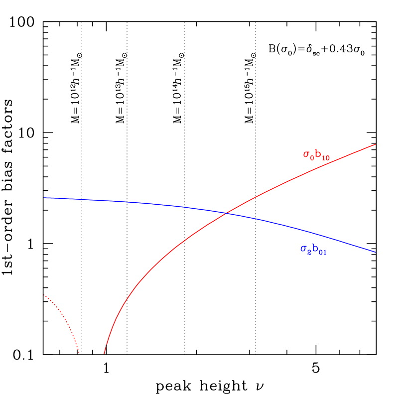
To illustrate the behaviour of the ESP bias parameters, we follow the methodology adopted in 2012arXiv1210.1483P . Namely, we smooth the density field with a tophat filter, while sticking to the Gaussian filter to define and (so that the second spectral moment remains finite). Therefore, we have , where the subscript and refer to tophat and Gaussian filtering, respectively, and denotes a mixed filtering, i.e. one filter is Gaussian and the other is tophat. Next, we construct the mapping between and by finding the for which . Finally, to account for departures from the spherical collapse approximation, we consider a moving barrier of the (square-root) form , where (2009ApJ…696..636R, ). For simplicity, we will ignore the scatter around even though it is quite substantial in the range of we are interested in. Fig.1 shows the first- and second-order peak bias factors at for a CDM cosmology with . Note that, while translate into a significance of , the actual height of density peaks is .
These results can be generalized to arbitrary filtering of the mass density field. For non-Gaussian initial conditions, there are a couple of subtleties which will be discussed elsewhere 111V. Desjacques, J.-O. Gong, A. Riotto, in preparation.
IV Discussion and Conclusions
We have shown that the 2-point correlation function of discrete density peaks can be computed, up to second order at least, from an effective local bias expansion in continuous fields that are invariant under rotations of the coordinate frame. This local expansion is not a count-in-cell relation in the sense that is merely an effective overdensity that can be used to recover the true from a trivial evaluation of . One of the consequences is that there only is one physically motivated smothing scale: the Lagrangian radius of the halos. Yet another important difference with the widespread local bias model is that one shall ignore all the contributions from zero-lag moments in order to obtain the correct .
All the bias coefficients can be derived from a peak-background split argument in which the background perturbation shifts the zero mean of the 1-point probability distribution functions of the rotationally invariant fields, unlike essentially all the other peak-background split formulations which consider a change in the number density of the tracers. Consequently, it is possible to derive bias factors from a peak-background split argument even if the variables are integrated over. The resulting probability densities can then be expanded in orthogonal polynomial bases. For the normally distributed peak height and curvature , these are bivariate Hermite polynomials whereas, for the chi-squared distributed and , these are generalized Laguerre polynomials. The peak bias factors are then obtained upon averaging the appropriate orthogonal polynomials over all the spatial locations that satisfy the peak constraint.
We have demonstrated that our simple local expansion reproduces the 2-point peak correlation function computed at second order by 2010PhRvD..82j3529D after a tedious expansion of the joint probability density . We believe that it should remain valid at higher orders. Furthermore, because discreteness enters the calculation only when averaging the orthogonal polynomials, we speculate that this local bias expansion combined with the peak-background split approach presented here can be generalized to describe the clustering of any point process of a Gaussian random field. The great advantage of our approach is that it circumvents the computation of , and requires only the evaluation of .
Our approach can be easily generalized to more sophisticated constraints involving, for instance, the tidal shear , where is the gravitational potential. As noted in 2002MNRAS.329…61S ; 2012arXiv1207.7117S , the quadratic invariant (the equivalent of our but with replaced by ) follows a -distribution with 5 degrees of freedom. Therefore, we expect that its associated bias parameters are given by some suitable average of the Laguerre polynomials . If the (nonspherical) collapse occurs at the spatial location of density peaks or includes the dependence on the large scale environment, then the distribution will be replaced by the appropriate conditional probability density 2008MNRAS.388..638D ; 2012MNRAS.421..296R , to which we shall apply the peak-background split in order to read off the new bias parameters.
Corrections induced by nonlinear gravitational evolution can also be decomposed into rotational invariants 1992ApJ…394L…5B ; 1995MNRAS.276…39C ; 2009JCAP…08..020M . Therefore, if one ignores the diffusion kernels (i.e. the propagators introduced by 2006PhRvD..73f3519C ), then it is straightforward to find explicit expressions for the Eulerian bias parameters in terms of local and nonlocal Lagrangian bias factors 1998MNRAS.297..692C ; 2012PhRvD..85h3509C ; 2012PhRvD..86h3540B ; 2012arXiv1207.7117S . This procedure can clearly be applied to our effective bias expansion Eq.(62), with the important caveat that discrete density peaks exhibit a statistical velocity bias. 2010PhRvD..81b3526D . Notwithstanding this, we expect from the structure of the kernel that the bias factors remain constant with time, in agreement with the findings of 2010PhRvD..82j3529D . For a more realistic treatment of gravitational motions, it should be possible to compute the evolved 2-point peak correlation in the framework of the integrated perturbation theory proposed by 2011PhRvD..83h3518M . We leave all this to future work.
Acknowledgments
I would like to thank Matteo Biagetti and Kwan Chuen Chan for their careful reading of the manuscript, and the Swiss National Science Foundation for support.
References
- (1) N. Kaiser, Astrophys. J. Lett.284, L9 (1984).
- (2) J. A. Peacock and A. F. Heavens, Mon. Not. R. Astron. Soc.217, 805 (1985).
- (3) J. M. Bardeen, J. R. Bond, N. Kaiser, and A. S. Szalay, Astrophys. J.304, 15 (1986).
- (4) V. Desjacques, M. Crocce, R. Scoccimarro, and R. K. Sheth, Phys. Rev. D82, 103529 (2010).
- (5) T. Matsubara, Astrophys. J.525, 543 (1999).
- (6) V. Desjacques, Phys. Rev. D78, 103503 (2008).
- (7) S. L. Lumsden, A. F. Heavens, and J. A. Peacock, Mon. Not. R. Astron. Soc.238, 293 (1989).
- (8) P. Coles, Mon. Not. R. Astron. Soc.238, 319 (1989).
- (9) V. Desjacques and R. K. Sheth, Phys. Rev. D81, 023526 (2010).
- (10) A. D. Ludlow and C. Porciani, Mon. Not. R. Astron. Soc.413, 1961 (2011).
- (11) A. Elia, A. D. Ludlow, and C. Porciani, Mon. Not. R. Astron. Soc.421, 3472 (2012).
- (12) A. Paranjape and R. K. Sheth, Mon. Not. R. Astron. Soc.426, 2789 (2012).
- (13) A. Paranjape, R. K. Sheth, and V. Desjacques, ArXiv e-prints (2012).
- (14) J. N. Fry and E. Gaztanaga, Astrophys. J.413, 447 (1993).
- (15) E. Regös and A. S. Szalay, Mon. Not. R. Astron. Soc.272, 447 (1995).
- (16) M. Kac, Bull. Am. Math. Soc. 49, 938 (1943).
- (17) S. O. Rice, Bell System Tech. J. 25, 46 (1945).
- (18) F. Schmidt, D. Jeong, and V. Desjacques, ArXiv e-prints (2012).
- (19) R. K. Sheth, K. C. Chan, and R. Scoccimarro, ArXiv e-prints (2012).
- (20) R. Dürrer, Fundamentals of Cosmic Physics 15, 209 (1994).
- (21) D. Pogosyan, C. Gay, and C. Pichon, Phys. Rev. D80, 081301 (2009).
- (22) R. K. Sheth and G. Tormen, Mon. Not. R. Astron. Soc.329, 61 (2002).
- (23) C. Gay, C. Pichon, and D. Pogosyan, Phys. Rev. D85, 023011 (2012).
- (24) H. J. Mo and S. D. M. White, Mon. Not. R. Astron. Soc.282, 347 (1996).
- (25) R. K. Sheth and G. Tormen, Mon. Not. R. Astron. Soc.308, 119 (1999).
- (26) M. L. Tiku, Biometrika 52, 415 (1965).
- (27) T. Matsubara, Phys. Rev. D83, 083518 (2011).
- (28) P. J. E. Peebles, Astrophys. J.196, 647 (1975).
- (29) S. D. M. White, Mon. Not. R. Astron. Soc.186, 145 (1979).
- (30) A. S. Szalay, Astrophys. J.333, 21 (1988).
- (31) M. Musso, A. Paranjape, and R. K. Sheth, ArXiv e-prints (2012).
- (32) T. Matsubara, Astrophys. J. Supp.101, 1 (1995).
- (33) M. Musso and R. K. Sheth, Mon. Not. R. Astron. Soc.423, L102 (2012).
- (34) L. Appel and B. J. T. Jones, Mon. Not. R. Astron. Soc.245, 522 (1990).
- (35) B. E. Robertson, A. V. Kravtsov, J. Tinker, and A. R. Zentner, Astrophys. J.696, 636 (2009).
- (36) V. Desjacques, Mon. Not. R. Astron. Soc.388, 638 (2008).
- (37) G. Rossi, Mon. Not. R. Astron. Soc.421, 296 (2012).
- (38) F. R. Bouchet, R. Juszkiewicz, S. Colombi, and R. Pellat, Astrophys. J. Lett.394, L5 (1992).
- (39) P. Catelan, F. Lucchin, S. Matarrese, and L. Moscardini, Mon. Not. R. Astron. Soc.276, 39 (1995).
- (40) P. McDonald and A. Roy, JCAP 8, 20 (2009).
- (41) M. Crocce and R. Scoccimarro, Phys. Rev. D73, 063519 (2006).
- (42) P. Catelan, F. Lucchin, S. Matarrese, and C. Porciani, Mon. Not. R. Astron. Soc.297, 692 (1998).
- (43) K. C. Chan, R. Scoccimarro, and R. K. Sheth, Phys. Rev. D85, 083509 (2012).
- (44) T. Baldauf, U. Seljak, V. Desjacques, and P. McDonald, Phys. Rev. D86, 083540 (2012).
Appendix A Computing correlators
For illustation, we evaluate the cross-covariance of the square modulus of the gradient at two different spatial locations and . We have
| (75) | ||||
where
| (76) |
To evaluate , we express in terms of the components of the unit vector, and take advantage of the fact that the integral over the angular variables is
| (77) |
Therefore, the product becomes (we omit the -dependence for conciseness)
| (78) |
which yields Eq.(29) once the multiplicative factor of and the additive zero-lag contribution are accounted for.
Appendix B Shape factor for peaks
In terms of the ordered eigenvalues of the hessian matrix , the asymmetry parameters that quantify the departure from a spherically symmetric peak density profile are and . The peak constraint together, with our choice of ordering, impose the four conditions , , and . Following 1986ApJ…304…15B , we also introduce an auxiliary function that measures the degree of asphericity expected for a peak,
| (79) |
This function scales as in the limit .
In 2010PhRvD..82j3529D , the peak 2-point correlation up to second order (i.e. terms quadratic in the correlation of the density field and its derivatives) is written as the sum of the linear contribution and three second-order terms , . In particular, contains all the terms for which the -dependence cannot be expressed as a polynomial in the linear and quadratic bias parameters . Their expression is phrased in terms of
| (80) |
and its integral over the th power of the peak curvature times the -dependent part of the one-point probability distribution,
| (81) |
These functions are very similar, albeit more general than those defined in Eqs (A15) and (A19) of 1986ApJ…304…15B .
Appendix C Non-central chi-squared distributions
The probability density of a non-central chi-squared distribution with degrees of freedom and non-centrality parameter is given by
| (82) |
where and is a modified Bessel function of the first kind. Ref. tiku:1965 proposed the following Laguerre polynomial expansion,
| (83) | ||||
The non-central -distribution can also be represented as a Poisson-weighted mixture of central -distributions (this was used by, e.g., 2012arXiv1207.7117S to estimate the nonlocal Lagrangian bias induced by ellipsoidal collapse). Note, however, that this representation does not make apparent the connection with the bias parameters .