Renormalization group flow equations connected to the $n$PI effective action

Abstract

In this paper we derive a hierarchy of integral equations from the 4PI effective action which have the form of Bethe-Salpeter equations. We show that the vertex functions defined by these equations can be used to truncate the exact renormalization group flow equations. This truncation has the property that the flow is a total derivative with respect to the flow parameter. We also show that the truncation is equivalent to solving the $n$PI equations of motion. This result establishes a direct connection between two non-perturbative methods.

I Introduction

There is much interest in the study of non-perturbative systems, which cannot be solved by exploiting the existence of a small expansion parameter. In this paper we discuss two formalisms that have been proposed to address non-perturbative problems: $n$-particle irreducible ($n$PI) effective theories Jackiw1974 ; Norton1975 , and the exact renormalization group (RG) Wetterich1993 ; Ellwanger1993 ; Tetradis1994 ; Morris1994 . The $n$PI formalism has been used to study finite temperature systems (see for example Blaizot1999 ; Berges2005a ), non-equilibrium dynamics and subsequent late-time thermalization (see Berges2001 and references therein), and transport coefficients Aarts2004 ; Carrington2008 ; Carrington2009 ; Carrington2010b . The exact RG has been applied to a variety of problems (for reviews see Morris-98 ; Bagnuls2001 ; Berges2002 ; Pawlowski2005 ; Delamotte2007 ; Rosten2007 ).

It has been proposed that the hierarchy of RG flow equations could be truncated at the level of the first equation using the Bethe-Salpeter (BS) equation derived from the 2PI effective action Blaizot2011 ; Blaizot2010 . The flow of the 2-point function is a total derivative with respect to the flow parameter, and the integral of the flow equation gives an integral equation whose solution is equivalent to the equation of motion (eom) for the 2-point function from the 2PI effective action. In this paper we show that the 4PI effective action produces two BS equations that can be used to truncate the RG flow equations at the level of the second equation, and that the resulting flow equations for the 2- and 4-point functions are total derivatives whose integrals give the 4PI eom’s. This result is surprising. Since the full hierarchy of RG flow equations are obtained using a single bi-local source term, one does not expect a connection to the nPI formalism beyond the lowest 2PI level. It suggests that a BS truncation at arbitrary orders produces equations whose integrals give the $n$PI eom’s, and establishes a direct connection between two non-perturbative methods. It also means that the truncation of the RG equations at any level of the hierarchy can be systematically extended by adding more and more skeleton diagrams to the effective action. For the $n$PI formalism, there could be a practical advantage in reformulating the integral equations as flow equations, because initial value problems are usually easier to solve than non-linear integral equations. Furthermore, regarding the vertices from the $n$PI effective theory as flow equations gives new insight into the problem of how to renormalize the $n$PI effective theory for $n>2$ Carrington2012 .

The paper is organized as follows. In section II we define our notation. In sections III and IV we give brief reviews of the RG flow equations and $n$PI effective action. In section V we review the derivation of the BS equation for the 4-point vertex from the 2PI effective action, and the procedure to use this equation to truncate the lowest order RG flow equation. In section VI we calculate the higher order BS equations that we will need, and in section VII we show how they can be used to truncate the renormalization group equations at higher orders. We present our conclusions in section VIII. Some details are left to the appendices.

II Notation

We work with a scalar field theory with quartic coupling and consider only the symmetric case where the expectation value of the field is zero. We define all propagators and vertices with factors of $i$ so that figures look as simple as possible: lines, and intersections of lines, correspond directly to propagators and vertices, with no additional factors of plus or minus $i$. The classical action is:

$$S[\varphi]=\int d^{d}x\bigg{(}\frac{1}{2}\varphi(x)^{2}-\frac{m^{2}}{2}\varphi(x)^{2}-\frac{i}{\;4!}\lambda\varphi(x)^{4}\bigg{)}\,,$$ (1)

and the bare propagator is defined:

$$G_{0}^{-1}(x,y)=-i\frac{\delta^{2}S[\varphi]}{\delta\varphi(x)\delta\varphi(y)}\,.$$ (2)

We use a compactified notation in which the space-time coordinates are represented by a single numerical subscript. For example, the propagator in equation (2) is written $G_{ij}:=G(x_{i},x_{j})$. We also use an Einstein convention in which a repeated index implies an integration over space-time variables. Using this notation we define the generating functionals:

$$Z[J]=\int d\varphi{\rm Exp}[i(S+J_{i}\varphi_{i})]\,,$$

$$W[J]=-i{\rm Ln}Z[J]\,,$$

$$\Gamma[\phi]=W[J]-J_{i}\frac{\delta W}{\delta J_{i}}\,.$$ (3)

The functional $W[J]$ is the generator of connected functions which are defined:

$$V^{c}_{x_{1},x_{2},x_{3},\cdots x_{k}}=\langle\varphi_{x_{1}}\varphi_{x_{2}}\varphi_{x_{3}}\dots\varphi_{x_{k}}\rangle_{c}=-(-i)^{k+1}\frac{\delta^{k}W}{\delta J_{x_{k}}\dots\delta J_{x_{3}}\delta J_{x_{2}}\delta J_{x_{1}}}\,.$$ (4)

The functional $\Gamma[\phi]$ generates 1-line irreducible, or proper, $n$-point functions. Using the notation $\Gamma=-i\Phi$ they are defined:

$$V_{x_{1},x_{2},x_{3},\cdots x_{k}} =\Phi^{(n)}(x_{1},x_{2},x_{3},\cdots x_{n})=\frac{\delta^{k}\Phi[\phi]}{\delta\phi_{x_{k}}\dots\delta\phi_{x_{3}}\delta\phi_{x_{2}}\delta\phi_{x_{1}}}\,.$$

Equations (2), (II) and (II) give

$$-\Phi^{(2)}(x,y)=G^{-1}(x,y)=G_{0}^{-1}-\Sigma(x,y)\,.$$ (5)

These $n$-point functions are invariant under translations of the co-ordinates and therefore in momentum space they depend on $n-1$ momenta. We use incoming momenta and the convention that the Fourier transformed $n$-point functions are defined without the 4-dimensional delta function that enforces the conservation of momentum:

$$(2\pi)^{d}\delta^{d}(p_{1}+p_{2}+\cdots p_{n})\Phi^{(n)}(p_{1},p_{2},\cdots p_{n})=\prod_{k=1}^{n}\int d^{d}x_{k}\;e^{i\sum_{j=1}^{n}p_{j}x_{j}}\;\Phi^{(n)}(x_{i}\cdots x_{n})\,.$$ (6)

We often use the shorthand notation:

$$\Phi^{(n)})(p_{1},p_{2},\cdots p_{n-1},-p_{1}-p_{2}-\cdots p_{n-1})=\Phi^{(n)})(p_{1},p_{2},\cdots p_{n-1})\,,$$ (7)

for example we write $\Phi^{(2)}(p,-p)=\Phi^{(2)}(p)=-G^{-1}(p)$.

III Renormalization group flow equations

In this section we give a brief summary of the RG flow equations (for reviews see Morris-98 ; Bagnuls2001 ; Berges2002 ; Pawlowski2005 ; Delamotte2007 ; Rosten2007 ). The RG is constructed by building a family of theories indexed by a continuous parameter $\kappa$ with the dimension of a momentum, such that fluctuations are smoothly taken into account as $\kappa$ is lowered from the microscopic scale $\Lambda$ (at which the couplings are defined) down to zero. To accomplish this, we add to the original action a non-local term which is quadratic in the fields:

$$\Delta S_{\kappa}[\varphi]=\frac{1}{2}\int dQ\,{\cal R}_{\kappa}(q)\varphi(q)\varphi(-q)\,,~{}~{}~{}dQ:=\frac{d^{d}q}{(2\pi)^{d}}\,.$$ (8)

The function ${\cal R}_{\kappa}$(q) is chosen so that it approaches zero for $q\gtrsim\kappa$ and $\kappa^{2}$ for $q\ll\kappa$. The first of these properties ensures that modes $\varphi(q\gtrsim\kappa)$ are unaffected, and the second suppresses the contribution of the modes $\varphi(q\ll\kappa)$ by giving them a mass $\sim\kappa$.

Generating functionals are defined as in equation (II) with the action $S$ replaced by $S+\Delta S_{\kappa}$, so that each generating functional now depends on the flow parameter $\kappa$. Differentiating with respect to $\kappa$ we obtain:

$$\partial_{\kappa}W_{\kappa}=\frac{1}{2}\int dQ\partial_{\kappa}{\cal R}_{\kappa}\langle\varphi(q)\varphi(-q)\rangle_{\kappa}=\frac{1}{2}\int dQ\partial_{\kappa}{\cal R}_{\kappa}G_{\kappa}(q,-q)\,,$$ (9)

where the subscript on the expectation value indicates that it depends on $\kappa$ (we remind the reader that we are considering the symmetric theory for which $\langle\varphi\rangle_{\kappa}=0$). It is easy to obtain the corresponding expression for the effective action. Using $\Phi_{\kappa}=i\Gamma_{\kappa}$ and defining $R_{\kappa}=i{\cal R}_{\kappa}$ we obtain:

$$\partial_{\kappa}\Phi_{\kappa}=\frac{1}{2}\int dQ\partial_{\kappa}R_{\kappa}\langle\varphi(q)\varphi(-q)\rangle_{\kappa}=\frac{1}{2}\int dQ\partial_{\kappa}R_{\kappa}G_{\kappa}(q,-q)\,,$$ (10)

and equation (5) becomes:

$$-G_{\kappa}^{-1}=R_{\kappa}+\Phi_{\kappa}^{(2)}\,,$$ (11)

which gives:

$$\partial_{\kappa}(G_{xy})_{\kappa}=(G_{xa})_{\kappa}\,\partial_{\kappa}(R_{\kappa}+\Phi_{\kappa}^{(2)})_{ab}\,(G_{by})_{\kappa}\,.$$ (12)

The diagrammatic notation we will use for equation (12) is shown in figure 1.

Figure 1: Diagrammatic representation of equation (12). The solid dot represents the insertion $\partial_{\kappa}R_{\kappa}$, the box with the cross is $\partial_{\kappa}\Phi_{\kappa}^{(2)}$, and the grey dot (red on-line) is the sum. Arrows on the ends of the lines indicate that propagator legs are attached.

Functionally differentiating equation (10) with respect to $\phi$ produces a hierarchy of equations known as the exact RG flow equations. The first two equations in this hierarchy are ($p_{4}=-p_{1}-p_{2}-p_{3}$):

$$\partial_{\kappa}\Phi_{\kappa}^{(2)}(p)= \frac{1}{2}\int dQ\,\partial_{\kappa}R_{\kappa}(q)G^{2}_{\kappa}(q)\Phi_{\kappa}^{(4)}(p,-p,q,-q)\,,$$ (13)

$$\partial_{\kappa}\Phi_{\kappa}^{(4)}(p_{1},p_{2},p_{3},p_{4})= \frac{1}{2}(6)\int dQ\,\Phi_{\kappa}^{(4)}(p_{1},p_{2},-q)G_{\kappa}(q)\partial_{\kappa}R_{\kappa}(q)G_{\kappa}(q)G_{\kappa}(p_{1}+p_{2}-q)\Phi_{\kappa}^{(4)}(q,p_{3},p_{4})$$ (14)

$$+\frac{1}{2}\int dQ\,G_{\kappa}(q)\partial_{\kappa}R_{\kappa}(q)G_{\kappa}(q)\Phi_{\kappa}^{(6)}(q,p_{1},p_{2},p_{3},p_{4})\,.$$

These equations are shown in figure 2. The factor (6) in equation (14) and figure 2 is a short-hand notation which means that there are 6 permutations of external legs only one of which is explicitly indicated. These correspond to the 4! ways to permute the 4 external legs of the diagram, divided by a factor 2$\cdot$2=4 to account for the fact that the vertices $\Phi_{\kappa}^{(4)}(p_{1},p_{2},-q)$ and $\Phi_{\kappa}^{(4)}(q,p_{3},p_{4})$ are symmetric under permutation of their legs. The 5 terms that are not written can be produced from the one which is using the variable changes: $p_{2}\leftrightarrow p_{1}$, $p_{2}\leftrightarrow p_{4}$, $\{p_{1},p_{2}\}\leftrightarrow\{p_{2},p_{3}\}$, $\{p_{1},p_{2}\}\leftrightarrow\{p_{2},p_{4}\}$, $\{p_{1},p_{2}\}\leftrightarrow\{p_{3},p_{4}\}$. Throughout this paper we will use this notation: numerical factors in brackets in equations (figures) represent additional terms that correspond to permutations of external indices that are not written (drawn).

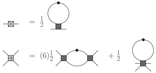
Figure 2: Diagrammatic representation of equations (13) and (14). Dark grey boxes with 2, 4 and 6 legs represent $\Phi_{\kappa}^{(2)}$, $\Phi_{\kappa}^{(4)}$ and $\Phi_{\kappa}^{(6)}$, respectively. Boxes with crosses through them (on the left side of the figure) represent the derivative with respect to the flow parameter of the corresponding vertex. The solid dot on a propagator represents the insertion $\partial_{\kappa}R_{\kappa}$.

The RG flow equations form an infinite coupled hierarchy: the equation for $\Phi^{(2n)}$ involves $\Phi^{(2)}$ and $\Phi^{(2[n+1])}$. In order to do calculations, one must truncate the hierarchy. This is a common feature of non-perturbative methods, and often leads to difficulties (see for example Smit2003 ; Zaraket2004 ; Binosi2009 ; Serreau2010 ).

IV The $n$PI effective action

The $n$PI effective action is obtained by taking the $n$th Legendre transform of the generating functional which is constructed by coupling the field to $n$ source terms:

$$Z[J,R,R^{(3)},R^{(4)},\dots]=\int d\varphi\;{\rm Exp}[i\,{\cal X}]\,,$$ (15)

$${\cal X}=S_{cl}[\varphi]+J_{i}\varphi_{i}+\frac{1}{2}R_{ij}\varphi_{i}\varphi_{j}+\frac{1}{3!}R^{(3)}_{ijk}\varphi_{i}\varphi_{j}\varphi_{k}+\frac{1}{4!}R^{(4)}_{ijkl}\varphi_{i}\varphi_{j}\varphi_{k}\varphi_{l}+\cdots\,,$$

$$W[J,R,R^{(3)},R^{(4)},\dots]=-i\,{\rm Ln}Z[J,R,R^{(3)},R^{(4)},\dots]\,,$$

$$\Gamma[\phi,G,U,V\dots]=W-J_{i}\frac{\delta W}{\delta J_{i}}-R_{ij}\frac{\delta W}{\delta R_{ij}}-R^{(3)}_{ijk}\frac{\delta W}{\delta R^{(3)}_{ijk}}-R^{(4)}_{ijkl}\frac{\delta W}{\delta R^{(4)}_{ijkl}}-\cdots$$

For future use we note the relations:

$$\frac{\delta W}{\delta J_{i}} =\langle\varphi_{i}\rangle=\phi_{i}\,,$$ (16)

$$2\frac{\delta W}{\delta R_{ij}} =\langle\varphi_{i}\varphi_{j}\rangle=G_{ij}+\phi_{i}\phi_{j}\,.$$ (17)

The $n$PI effective action is obtained from the last line of Eq. (15) and can be written:

$$\Gamma[\phi,G,U,V\dots] =-i\Phi[\phi,G,U,V\dots]$$

$$=S_{cl}[\phi]+\frac{i}{2}{\rm Tr}\,{\rm Ln}G^{-1}+\frac{i}{2}{\rm Tr}\left[\left(G^{0}\right)^{-1}G\right]-i\Phi_{2}[\phi,G,U,V\dots]~{}~{}+~{}~{}{\rm const}\,.$$

The term $\Phi_{2}[\phi,G,U,V\dots]$ contains all contributions to the effective action which have two or more loops. For example, for the 4-Loop 4PI effective action Berges2004 ; Carrington2004 ; Carrington2010b in the symmetric theory $\Phi_{2}$ is shown in figure 3.

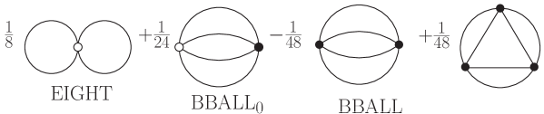
Figure 3: The functional $\Phi_{2}$ for the 4-Loop 4PI effective action. Bare vertices are denoted by open circles and effective vertices are solid dots.

The self consistent propagator and vertex are obtained through the variational principle by solving the equations produced by taking the functional derivative of the effective action and setting the result to zero. For the 4PI effective theory this gives:

$$-\frac{\delta\Phi}{\delta G_{xy}}=-G^{-1}_{xy}+(G^{-1}_{0})_{xy}-\Sigma_{xy}=0\,,~{}~{}~{}\Sigma_{xy}=2\frac{\delta\Phi_{2}}{\delta G_{xy}}\,,$$ (19)

$$4!G^{-1}_{xx^{\prime}}G^{-1}_{xx^{\prime}}G^{-1}_{xx^{\prime}}\frac{\delta\Phi}{\delta V_{x^{\prime}y^{\prime}w^{\prime}z^{\prime}}}=-V_{xywz}+\lambda\delta_{xy}\delta_{xw}\delta_{xz}+4!G^{-1}_{xx^{\prime}}G^{-1}_{yy^{\prime}}G^{-1}_{ww^{\prime}}G^{-1}_{zz^{\prime}}\frac{\delta\hat{\Phi}_{2}}{\delta V_{x^{\prime}y^{\prime}w^{\prime}z^{\prime}}}=0\,.$$ (20)

The minus sign on the left side of equation (19) is related to the minus sign in equation (5) and is discussed in footnote 1. The term $-G^{-1}_{xy}$ comes from the 1-loop terms in the effective action and is moved to the other side of the equation to produce the usual form of the Dyson equation. This is shown in figure 4. In equation (20) the term $-V_{xywz}$ is produced by the basketball (BBALL) diagram in figure 3 and is moved to the other side to produce the equation of motion shown in figure 5.

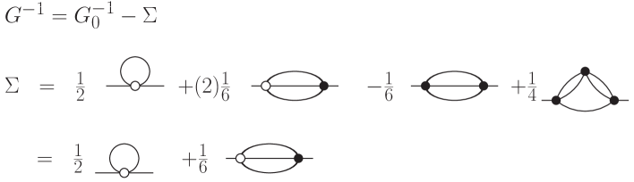
Figure 4: Equation of motion for the self-energy from the 4-Loop 4PI effective action. The second line illustrates the notation we use throughout this paper in which different permutations of external indices are indicated with a bracketed numerical factor. In the third line we have used the equation of motion for the 4-point function which is shown in figure 5.

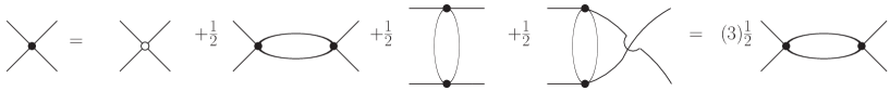
Figure 5: Equation of motion for the 4-point function from the 4-Loop 4PI effective action. In the last section of the figure different permutations of external indices are indicated with a bracketed numerical factor.

V Lowest order truncation

V.1 Bethe-Salpeter equation from the 2PI effective action

It is well known that the 2PI effective action can be used to obtain a 4-point vertex called the Bethe-Salpeter vertex vanHees2002 . In this section we review the derivation of this equation. We calculate the functional derivative of the effective action with respect to the 2-point function $G_{kl}$ and the source $R_{ij}$. We do the calculation in two different ways and equate the results. First, we use the last line in equation (15) with the derivatives $\delta W/\delta J$ and $\delta W/\delta R$ written in terms of the expectation value and propagator using equation (16). Differentiating we obtain:

$$\frac{\delta}{\delta R_{ij}}\frac{\delta}{\delta G_{kl}}\Phi =i\frac{\delta}{\delta R_{ij}}\bigg{(}\frac{\delta J_{x}}{\delta G_{kl}}\frac{\delta W}{\delta J_{x}}+\frac{\delta R_{xy}}{\delta G_{kl}}\frac{\delta W}{\delta R_{xy}}-\frac{\delta J_{x}}{\delta G_{kl}}\phi_{x}$$ (21)

$$-\frac{1}{2}\frac{\delta R_{xy}}{\delta G_{kl}}\big{(}G_{xy}+\phi_{x}\phi_{y}\big{)}-\frac{1}{4}R_{xy}(\delta_{xk}\delta_{yl}+\delta_{xl}\delta_{yk})\bigg{)}\,.$$

Using (16) the first and third, and the second and fourth terms on the right side cancel identically, and we are left with:

$$\frac{\delta}{\delta R_{ij}}\frac{\delta}{\delta G_{kl}}\Phi=-\frac{i}{4}\big{(}\delta_{ik}\delta_{jl}+\delta_{il}\delta_{jk}\big{)}\,.$$ (22)

Now we repeat the calculation using equation (IV) for the effective action. We obtain:

$$\frac{\delta}{\delta R_{ij}}\frac{\delta}{\delta G_{kl}}\Phi=\frac{\delta\phi_{x}}{\delta R_{ij}}\frac{\delta^{2}\Phi}{\delta\phi_{x}\delta G_{kl}}+\frac{\delta G_{xy}}{\delta R_{ij}}\frac{\delta^{2}\Phi}{\delta G_{xy}\delta G_{kl}}\,.$$ (23)

Since we consider only the symmetric theory, we drop all terms that correspond to vertices with an odd number of legs, which means that only the second term on the right side survives. Using (IV) we write:

$$4\frac{\delta^{2}\Phi}{\delta G_{xy}\delta G_{kl}} =4\frac{\delta^{2}(\Phi-\Phi_{2})}{\delta G_{xy}\delta G_{kl}}+4\frac{\delta^{2}\Phi_{2}}{\delta G_{xy}\delta G_{kl}}\,,$$ (24)

$$=:\Lambda^{disco}_{xykl}+\Lambda_{xykl}=-(G^{-1}_{xk}G^{-1}_{yl}+G^{-1}_{xl}G^{-1}_{yk})+\Lambda_{xykl}\,.$$

The term $\Lambda^{disco}_{xykl}$ represents all disconnected contributions and comes from the 1-loop terms in the effective action, and $\Lambda_{xykl}$ contains all contributions from $\Phi_{2}$.

The last step is to calculate the derivative of the propagator with respect to the source $R$. We have:

$$\frac{\delta G_{xy}}{\delta R_{ij}} =\frac{\delta}{\delta R_{ij}}\big{(}\langle\varphi_{x}\varphi_{y}\rangle-\langle\varphi_{x}\rangle\langle\varphi_{y}\rangle\big{)}\,,$$ (25)

$$=\frac{i}{2}\big{(}\langle\varphi_{x}\varphi_{y}\varphi_{i}\varphi_{j}\rangle-\langle\varphi_{x}\varphi_{y}\rangle\langle\varphi_{i}\varphi_{j}\rangle~{}+~{}\cdots\big{)}\,,$$

$$=\frac{i}{2}\big{(}G_{ia}G_{jb}G_{xc}G_{yd}V_{abcd}+G_{ix}G_{jy}+G_{iy}G_{jx}~{}+~{}\cdots\big{)}\,,$$

where the dots indicate expectation values which contain an odd number of field operators and are dropped since we are considering the symmetric theory.

We substitute equations (24) and (25) into (23) and set the result equal to the expression obtained in (22). This procedure gives:

$$0=\frac{i}{4}G_{ix}G_{jy}\,\big{(}-V_{klxy}+\Lambda_{klxy}+\frac{1}{2}\Lambda_{klab}G_{ac}G_{bd}V_{cdxy}\big{)}\,,$$ (26)

where we have used the fact that the vertex $V_{klxy}$ is symmetric with respect to permutations of any pair of indices, and the vertex $\Lambda_{klxy}$ is symmetric with respect to permutations of the first two indices, or the second two indices, or the interchange of the first pair and the second pair: $\Lambda_{klxy}=\Lambda_{lkxy}=\Lambda_{klyx}=\Lambda_{xykl}$. Truncating the external legs we obtain the standard form of the BS equation:

$$V_{xykl}=\Lambda_{xykl}+\frac{1}{2}\Lambda_{xyab}G_{ac}G_{bd}V_{cdkl}\,.$$ (27)

We consider systems in thermal equilibrium for which the system is invariant under space-time translations. In this case equation (27) can be written in momentum space as:

$$V(p,-p,q,-q)=\Lambda(p,-p,q,-q)+\frac{1}{2}\int dK\,\Lambda(p,-p,k,-k)G^{2}(k)V(k,-k,q,-q)\,.$$ (28)

Due to the translation invariance of the propagator, the 4-point function does not have general momentum arguments, but rather is restricted to the particular configuration indicated in equation (28). We will refer to these momentum arguments as “diagonal.” Equation (28) is shown diagrammatically in figure 6.

Figure 6: Diagrammatic representation of the BS equation in equation (28). Boxes and circles represent the vertex $V$ and kernel $\Lambda$, respectively.

V.2 Truncation of the lowest order renormalization group equation

It has been proposed that the hierarchy of RG flow equations could be truncated using the BS equation derived in the previous section Blaizot2011 ; Blaizot2010 . The procedure is as follows. We extend equation (28) to the deformed theory by writing:

$$V_{\kappa}(p,-p,q,-q)=\Lambda_{\kappa}(p,-p,q,-q)+\frac{1}{2}\int dK\,\Lambda_{\kappa}(p,-p,k,-k)G_{\kappa}^{2}(k)V_{\kappa}(k,-k,q,-q)\,.$$ (29)

In this equation the subscript on $\Lambda_{\kappa}$ indicates that the functional derivative which defines the kernel is taken with respect to the propagator, and the kernel is then evaluated at $G=G_{\kappa}$ (as defined in equation (11)). If we use $\Phi^{(4)}_{\kappa}=V_{\kappa}$ the equations (13) and (29) form a closed set. If the full effective action is used, the solution of this coupled system of equations gives the full 2-point function, and the full 4-point function for diagonal momenta. This observation points out an important feature of the truncation: it can be systematically extended by adding more and more skeleton diagrams to the effective action.

The result of the truncation is easiest to see diagrammatically and is shown in figure 7. In the first line of this figure we replace the dark grey box in the tadpole diagram in figure 2 (which represents $\Phi_{\kappa}^{(4)}$) by the light grey box on the left side of figure 6 (which represents $V_{\kappa}$). Using right side of figure 6 we obtain the second line of figure 7. The box of dotted lines is just the insertion $2\partial_{\kappa}\Phi_{\kappa}^{(2)}$, using the first line of the figure. Inserting the first line into the second we obtain the first part of the third line. In the second part of the third line we use the notation in figure 1 to represent the sum of terms $\partial_{\kappa}R_{\kappa}+\partial_{\kappa}\Phi^{(2)}$ by a small grey dot (red on-line).

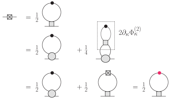
Figure 7: The result obtained using the BS equation from section V.1 to truncate the first RG flow equation in (13).

An interesting aspect of this truncation is that it has the property that the flow is a total derivative with respect to the flow parameter $\kappa$. To prove this, we consider the 2-point function obtained from the 2PI effective action. Using equation (19) and evaluating at $G=G_{\kappa}$ after taking the functional derivative we obtain:

$$(\Sigma_{ij})_{\kappa}=2\frac{\delta\Phi_{2}}{\delta G_{ij}}\bigg{|}_{G_{\kappa}}=\Sigma_{ij}[G_{\kappa}]\,,$$ (30)

and therefore:

$$\partial_{\kappa}(\Sigma_{ij})_{\kappa} =2\partial_{\kappa}(G_{kl})_{\kappa}\frac{\delta^{2}\Phi_{2}}{\delta G_{kl}\delta G_{ij}}\bigg{|}_{G_{\kappa}}=\frac{1}{2}\partial_{\kappa}(G_{kl})_{\kappa}(\Lambda_{ijkl})_{\kappa}\,,$$ (31)

$$=\frac{1}{2}\big{[}(G_{ka})_{\kappa}\partial_{\kappa}(R_{ab}+\Phi^{(2)}_{ab})(G_{bj})_{\kappa}\big{]}(\Lambda_{ijkl})_{\kappa}\,,$$

where we used equations (24) and (12) in the first and second lines. Equation (31) is exactly the result for $\partial_{\kappa}\Phi_{\kappa}^{(2)}$ that is shown in the last line of figure 7 and therefore we have obtained:

$$\partial_{\kappa}\Phi_{\kappa}^{(2)}=\partial_{\kappa}\Sigma_{\kappa}\,.$$ (32)

Thus we have shown that the flow is a total derivative with respect to the flow parameter, and the integral of the flow equation gives an integral equation whose solution is equivalent to the equation of motion for the 2-point function from the 2PI effective action.

VI Higher order BS equations

In this section we derive some higher order Bethe-Salpeter type equations from the 2PI and 4PI equations of motion. In the next section we will show how to use these equations to truncate the RG hierarchy at higher orders. Throughout this paper we use circles to denote kernels and boxes are vertices obtained by solving integral equations.

VI.1 Kernel notation

We introduce some notation for the various kernels that we will encounter:

$$\Lambda^{\rm disco}_{abcd\cdots rstuvxyz\cdots}+\Lambda_{abcd\cdots rstuvxyz\cdots}=2^{\#G}4!^{\#V}\big{(}G^{-1}_{rr^{\prime}}\cdots G^{-1}_{zz^{\prime}}\big{)}\frac{\delta^{(\#G)+(\#V)}\Phi}{\delta G_{ab}\delta G_{cd}\cdots\delta V_{r^{\prime}s^{\prime}t^{\prime}u^{\prime}}\delta V_{v^{\prime}x^{\prime}y^{\prime}z^{\prime}}\cdots}$$ (33)

The factors ${\#G}$ and ${\#V}$ indicate the number of $G$’s and $V$’s with respect to which the functional derivatives are taken. The inverse propagators truncate the legs that are left behind by the functional derivatives with respect to $V$ (there are $4\cdot({\#V})$ inverse propagators in total) which produces an amputated kernel. The definition of the kernel $\Lambda_{ab\cdots}$ excludes the disconnected contribution because this piece will always cancel in BS equations. For $\#G=2$ and $\#V=0$ equation (33) reduces to (24).

Note that the kernels defined in (33) for the cases where only one derivative is taken are not really kernels, since the right side is just the equation of motion for the corresponding vertex. In this case we obtain an integral equation by moving the vertex to the other side of the equation, as explained under equation (20).

Above equation (27) we commented on the symmetries of the 4-point vertex $\Lambda_{abcd}$ with respect to interchange of leg indices. In general, the vertices in equation (33) are symmetric with respect to the interchange of any two co-ordinates which came from the same $G$ or $V$ in the functional derivative. In addition, if there is more than one $G$ or $V$, one can interchange the full set of corresponding indices (in any order). For example, consider the 8-point kernel:

$$\Lambda^{\rm disco}_{abcdrstu}+\Lambda_{abcdrstu}=2^{2}4!\big{(}G^{-1}_{rr^{\prime}}G^{-1}_{ss^{\prime}}G^{-1}_{tt^{\prime}}G^{-1}_{uu^{\prime}}\big{)}\frac{\delta^{3}\Phi}{\delta G_{ab}\delta G_{cd}\delta V_{r^{\prime}s^{\prime}t^{\prime}u^{\prime}}}\,.$$ (34)

Some permutations of the variables $\{a,b,c,d,r,s,t,u\}$ that produce the same vertex are: $a\leftrightarrow b$, $r\leftrightarrow s$ and $\{a,b\}\leftrightarrow\{c,d\}$. Two permutations that do not are $a\leftrightarrow c$ and $a\leftrightarrow r$.

In equilibrium, translation invariance means that the kernels will depend only on the differences of the co-ordinate indices of each element of the functional derivative. For example, the vertex in (34) does not depend on $x_{a}$ and $x_{b}$ individually, but only on the difference $x_{a}-x_{b}$. Similarly, it does not depend on $x_{r}$, $x_{s}$, $x_{t}$ and $x_{u}$ but only on (for example) $x_{r}-x_{u}$, $x_{s}-x_{u}$ and $x_{t}-x_{u}$. The consequence of this invariance is that in momentum space the kernel does not have a number of independent momentum arguments equal to the number of its legs. For example, the Fourier transform of the vertex in equation (34) has the form $\Lambda(p,-p,k,-k,q_{1},q_{2},q_{3},-q_{1}-q_{2}-q_{3})$ (using the shorthand notation introduced in equation (7) we sometimes write $\Lambda(p,k,q_{1},q_{2},q_{3})$). Using $\#G=2$ and $\#G=3$ we obtain 4- and 6-point kernels which have diagonal momentum arguments of the form $\Lambda(p,-p,q,-q)$ and $\Lambda(p,-p,q,-q,k,-k)$. Using $\#G=1$ and $\#V=1$ produces a 6-point kernel with momentum arguments $\Lambda(p,-p,q_{1},q_{2},q_{3},-q_{1}-q_{2}-q_{3})$ which we will call partially-diagonal. Thus the general 6-point function depends on 5 independent momenta, and the partially-diagonal and diagonal 6-point functions depend on 4 and 3 independent momenta, respectively. Note that we always use the convention that the delta functions that enforce the conservation of momentum are removed from the Fourier transformed vertex (see equation (6)).

VI.2 BS equation for a 6-point vertex from the 2PI effective action

One can obtain a BS equation for a 6-point vertex from the 2PI effective action using the method that was used in section V.1 for the 4-point function. To obtain a 6-point vertex we calculate the functional derivative $\delta^{3}\Phi/\delta R\delta R\delta G$. Using the chain rule we have:

$$0=\frac{\delta^{3}\Phi}{\delta R_{ab}\delta R_{cd}\delta G_{ef}}=\frac{\delta^{2}G_{xy}}{\delta R_{ab}\delta R_{cd}}\;\frac{\delta^{2}\Phi}{\delta G_{xy}\delta G_{ef}}+\frac{\delta G_{xy}}{\delta R_{cd}}\;\frac{\delta G_{rs}}{\delta R_{ab}}\;\frac{\delta^{3}\Phi}{\delta G_{rs}\delta G_{xy}\delta G_{ef}}\,,$$ (35)

where the zero on the left side is obtained from equation (22). Using equation (33) the second derivative of the effective action with respect to the propagator gives the kernel $\frac{1}{4}(\Lambda^{\rm disco}_{xyef}+\Lambda_{xyef})$ and the third derivative gives:

$$8\frac{\delta^{3}\Phi}{\delta G_{rs}\delta G_{xy}\delta G_{ef}} =\Lambda^{\rm disco}_{rsxyef}+\Lambda_{rsxyef}\,.$$ (36)

The disconnected contribution comes from the functional derivatives acting on the 1-loop piece of the effective action and is:

$$\Lambda^{\rm disco}_{rsxyef} =-(G^{-1}_{ey}G^{-1}_{fs}G^{-1}_{rx}+G^{-1}_{ey}G^{-1}_{fr}G^{-1}_{sx}+G^{-1}_{es}G^{-1}_{fy}G^{-1}_{rx}+G^{-1}_{er}G^{-1}_{fy}G^{-1}_{sx}$$ (37)

$$~{}~{}~{}+G^{-1}_{ex}G^{-1}_{fs}G^{-1}_{ry}+G^{-1}_{es}G^{-1}_{fx}G^{-1}_{ry}+G^{-1}_{ex}G^{-1}_{fr}G^{-1}_{sy}+G^{-1}_{er}G^{-1}_{fx}G^{-1}_{sy})$$

$$=(8)G^{-1}_{ey}G^{-1}_{fs}G^{-1}_{rx}\,.$$

There are eight terms which correspond to the eight ways to group the indices $\{r,s,x,y,e,f\}$ into the three factors of inverse propagators, excluding terms of the form $G^{-1}_{ij}$ where $\{i,j\}=\{r,s\}$ or $\{x,y\}$ or $\{e,f\}$. In the last line of equation (36) we use the notation introduced in section III and write only one term, indicating that there are eight terms in total with the factor (8).

The functional derivative $\delta G/\delta R$ is calculated in section V.1 and the result is given in equation (25). The method to obtain the second derivative is exactly analogous. Starting from the expression in equation (25) and taking an additional derivative we obtain:

$$-4\frac{\delta}{\delta R_{cd}}\frac{\delta G_{xy}}{\delta R_{ab}} =\langle\varphi_{c}\varphi_{d}\varphi_{a}\varphi_{b}\varphi_{x}\varphi_{y}\rangle-\langle\varphi_{c}\varphi_{d}\rangle\langle\varphi_{a}\varphi_{b}\varphi_{x}\varphi_{y}\rangle$$ (38)

$$-\langle\varphi_{c}\varphi_{d}\varphi_{x}\varphi_{y}\rangle\langle\varphi_{a}\varphi_{b}\rangle+\langle\varphi_{c}\varphi_{d}\rangle\langle\varphi_{x}\varphi_{y}\rangle\langle\varphi_{a}\varphi_{b}\rangle$$

$$-\langle\varphi_{x}\varphi_{y}\rangle\langle\varphi_{c}\varphi_{d}\varphi_{a}\varphi_{b}\rangle+\langle\varphi_{c}\varphi_{d}\rangle\langle\varphi_{x}\varphi_{y}\rangle\langle\varphi_{a}\varphi_{b}\rangle\,.$$

Converting to connected functions the right side of (38) becomes:

$$V^{c}_{abcdxy} +G_{ay}V^{c}_{bcdx}+G_{dy}V^{c}_{abcx}+G_{cy}V^{c}_{abdx}+G_{by}V^{c}_{acdx}+G_{dx}V^{c}_{abcy}+G_{cx}V^{c}_{abdy}+G_{bx}V^{c}_{acdy}$$ (39)

$$+G_{ax}V^{c}_{bcdy}+G_{bd}V^{c}_{acxy}+G_{ad}V^{c}_{bcxy}+G_{bc}V^{c}_{adxy}+G_{ac}V^{c}_{bdxy}+G_{ay}G_{bd}G_{cx}+G_{ay}G_{bc}G_{dx}$$

$$+G_{ad}G_{by}G_{cx}+G_{ac}G_{by}G_{dx}+G_{ax}G_{bd}G_{cy}+G_{ad}G_{bx}G_{cy}+G_{ax}G_{bc}G_{dy}+G_{ac}G_{bx}G_{dy}\,.$$

Combining permutations of external indices to make this result more compact we write:

$$-4\frac{\delta^{2}G_{xy}}{\delta R_{cd}\delta R_{ab}} =V^{c}_{xyabcd}+(8)V^{c}_{xabc}G_{yd}+(4)V^{c}_{xyab}G_{cd}+(8)G_{xa}G_{yb}G_{cd}\,.$$ (40)

Substituting equations (24), (25), (36) and (39) into (35) produces a lengthy expression that can be manipulated into a compact form. The result is shown in figure 8, and some details are given in Appendix A. In equilibrium the expression depends only on the differences of co-ordinates $(x_{a}-x_{b})$, $(x_{c}-x_{d})$ and $(x_{e}-x_{f})$, and in momentum space it depends on only 3 momenta. For example, the momentum dependence of the vertex $\Lambda_{abcdef}$ (the second diagram on the right side of figure 8) is shown in figure 9.

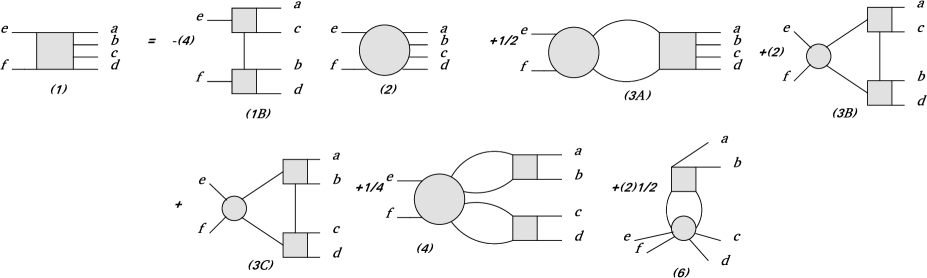
Figure 8: The BS equation for 6-point vertex function from the 2PI effective action. The numbers under each graph refer to the discussion in Appendix A.

Figure 9: Part (2) of figure 8 with co-ordinate indices and momentum arguments for each leg.

We note that the BS equations in figures 6 and 8 do not form a closed set, since the diagrams (1B) and (3B) in figure 8 contain non-diagonal 4-point vertices. In section VII.1 we will show that, in spite of this, these BS equations can be used to truncate the RG equations at the level of the second equation, because of the fact that the vertex $\Phi_{\kappa}^{(4)}$ also contains non-diagonal 4-point vertices.

VI.3 BS equations from the 4PI effective action

In this section we obtain two BS type integral equations from the 4PI effective action. Throughout this paper, in order to avoid a proliferation of indices, we do not introduce additional subscripts to distinguish the 2PI and 4PI effective actions and the vertices obtained from them.

We can obtain the BS equation for a diagonal 4-point function from the 4PI effective action, following the technique in section V.1, by calculating the functional derivative $\delta^{3}\Phi/\delta R\delta G$ where $\Phi$ is the 4PI effective action instead of the 2PI one. In section V.1 the integral equation for the 4-vertex was obtained by comparing the results of equations (22) and (23). Using the 4PI effective action, equation (21) contains two additional terms produced by the source $R^{(4)}$, but it is easy to see that the result in equation (22) is unchanged. Equation (23) becomes (in the symmetric theory):

$$\frac{\delta}{\delta R_{ij}}\frac{\delta}{\delta G_{kl}}\Phi=\frac{\delta G_{xy}}{\delta R_{ij}}\frac{\delta^{2}\Phi}{\delta G_{xy}\delta G_{kl}}+\frac{\delta V_{xywz}}{\delta R_{ij}}\frac{\delta^{2}\Phi}{\delta V_{xywz}\delta G_{kl}}\,.$$ (41)

Using equation (33) the two terms on the right side contain the kernels $\frac{1}{4}(\Lambda^{\rm disco}_{xykl}+\Lambda_{xykl})$ and $\frac{1}{2}\frac{1}{4!}\Lambda_{xywzkl}$ (note that the kernel obtained from $\delta\Phi/\delta G\delta V$ does not have a disconnected piece). The derivative $\delta G/\delta R$ is calculated in section V.1 and given in equation (25). The derivative $\delta V/\delta R$ can be calculated in exactly the same way. Some details are found in Appendix B, the result is given in equation (57). Substituting the expressions for the derivatives we obtain the result in figure 10.

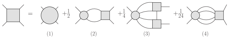
Figure 10: The BS equation that is produced by the functional derivative $\delta\Phi/\delta R_{ij}\delta G_{kl}$ where $\Phi$ is the 4PI effective action. Legs on the left side of the figure have indices $(k,l)$ and in momentum space they carry momenta $\pm p$. The legs on the right side have indices $(i,j)$ and carry momenta $\pm q$.

We can also obtain a BS equation for a partially-diagonal 6-point function of the form $V(p,-p,k_{1},k_{2},k_{3},-k_{1}-k_{2}-k_{3})$ by calculating the functional derivative $\delta\Phi/\delta R\delta V$ where $\Phi$ is the 4PI effective action. Using the chain rule we obtain:

$$0=\frac{\delta^{2}\Phi}{\delta R_{ab}\delta V_{cdef}}=\frac{\delta G_{xy}}{\delta R_{ab}}\;\frac{\delta^{2}\Phi}{\delta G_{xy}\delta V_{cdef}}+\frac{\delta V_{xywz}}{\delta R_{ab}}\;\frac{\delta^{2}\Phi}{\delta V_{xywz}\delta V_{cdef}}\,,$$ (42)

where the zero on the left side comes from equation (22). The functional derivatives of the effective action give the kernels (see equation (33)):

$$2\cdot 4!\,\frac{\delta^{2}\Phi}{\delta G_{xy}\delta V_{cdef}}=G_{cc^{\prime}}G_{dd^{\prime}}G_{ee^{\prime}}G_{ff^{\prime}}\big{(}\Lambda_{xyc^{\prime}d^{\prime}e^{\prime}f^{\prime}}\big{)}\,,$$

$$4!\cdot 4!\,\frac{\delta^{2}\Phi}{\delta V_{xywz}\delta V_{cdef}}=G_{xx^{\prime}}G_{yy^{\prime}}G_{ww^{\prime}}G_{zz^{\prime}}G_{cc^{\prime}}G_{dd^{\prime}}G_{ee^{\prime}}G_{ff^{\prime}}\big{(}\Lambda^{\rm disco}_{x^{\prime}y^{\prime}w^{\prime}z^{\prime}c^{\prime}d^{\prime}e^{\prime}f^{\prime}}+\Lambda_{x^{\prime}y^{\prime}w^{\prime}z^{\prime}c^{\prime}d^{\prime}e^{\prime}f^{\prime}}\big{)}\,.$$ (43)

The kernel obtained from $\delta\Phi/\delta G\delta V$ does not contain a disconnected piece. The kernel from $\delta\Phi/\delta V\delta V$ does have a disconnected piece which is produced by the basketball diagram. The derivative $\delta G_{xy}/\delta R_{ab}$ is given in equation (25) and $\delta V_{xywz}/\delta R_{ab}$ is calculated in Appendix B. To obtain the BS equation we substitute (25), (43) and (57) into (42). After a tedious but straightforward calculation we obtain the result in figure 11.

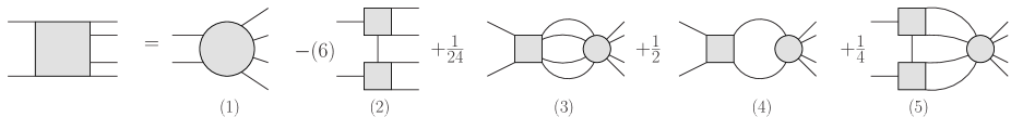
Figure 11: The BS equation that is produced by the functional derivative $\delta\Phi/\delta R_{ab}\delta V_{xywz}$. Legs on the left side of the figure have indices $(a,b)$ and in momentum space they carry momenta $\pm p$. The legs on the right side have indices $(x,y,w,z)$ and carry momenta $(k_{1},k_{2},k_{3},-k_{1}-k_{2}-k_{3})$.

VII Higher order truncations

VII.1 Truncation at the second level using the 2PI effective action

In this section we consider the truncation of the RG flow equations at the level of the second equation using integral equations obtained from the 2PI effective action (figures 6 and 8) and following the same procedure as in section V. The truncation can only be done if we restrict the second RG flow equation (equation (14)) to diagonal external momenta and consider only 4-point functions of the form $\Phi_{\kappa}^{(4)}(p,-p,q,-q)$, so that the 6-point function that appears in the tadpole diagram has diagonal momentum arguments of the form $\Phi_{\kappa}^{(6)}(p,-p,q,-q,k,-k)$. The BS equations have kernels with four and six legs of the form $\Lambda_{ijkl}=4\delta\Phi/\delta G_{ij}\delta G_{kl}$ and $\Lambda_{ijklrs}=8\delta\Phi/\delta G_{ij}\delta G_{kl}\delta G_{rs}$ which can be extended to the deformed theory by taking functional derivatives of the effective action and then evaluating at $G=G_{\kappa}$. This produces BS 4- and 6-point vertices that depend on the flow parameter. We show below how to truncate the hierarchy of RG equations at the level of the second equation by replacing the vertices $\Phi_{\kappa}^{(4)}$ and $\Phi_{\kappa}^{(6)}$ with the corresponding BS vertices.

We start by substituting the BS equation in figure 8 into the tadpole graph in the second line of figure 2. This produces the set of graphs in figure 12. The diagram labelled (1B) cancels the $t$- and $u$-channels from the bubble graph in the second line of figure 2. The remaining $s$-channel diagram can be rewritten by replacing the 4-vertex $\Phi^{(4)}_{\kappa}$ on the left side with the BS vertex $V_{\kappa}$ in figure 6 . The result is shown in figure 13. Combining the results in figures 12 and 13 gives the result in figure 14, where we have used the notation in figure 1 to represent the sum of terms $\partial_{\kappa}R_{\kappa}$ (represented by a black dot) and $\partial_{\kappa}\Phi^{(2)}$ by a small grey dot (red on-line).

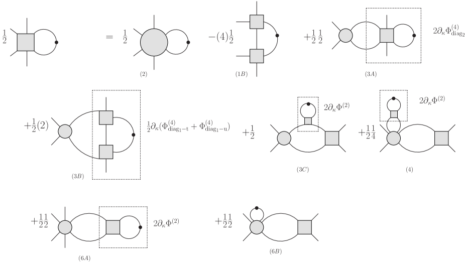
Figure 12: The tadpole diagram from the second RG flow equation with diagonal momenta and the 6-point vertex replaced using the BS equation in figure 8. In each diagram, the legs on the left side have co-ordinate indices $(e,f)$ and carry momenta $\pm p$. The remaining legs have co-ordinate indices $(c,d)$ and momenta $\pm k$. The dotted boxes indicate combinations that can be replaced by re-substituting the RG flow equations. The notation $\partial_{\kappa}\Phi^{(4)}_{{\rm diag_{2}}}$ indicates the second diagram on the right side of the second RG equation in figure 2, $\partial_{\kappa}\Phi^{(4)}_{{\rm diag_{1}}-t}$ indicates the $t$-channel of the first diagram, etc. The number under each diagram indicates the term in figure 8 that produced it. The graph labelled (6) in figure 8 produces two different contributions (6A) and (6B), which correspond respectively to the diagrams in (6) with $(c,d)$ and $(a,b)$ attached to the kernel.

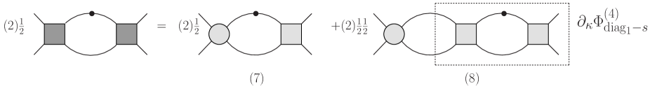
Figure 13: The surviving s-channel bubble diagram from the second RG flow equation with the left 4-point vertex replaced using the BS equation in figure 6. The dotted box on the right side indicates a combination that can be rewritten using the second RG flow equation.

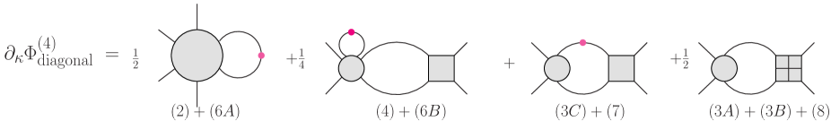
Figure 14: The result obtained by combining the surviving diagrams in figures 12 and 13. The subscript “diagonal” indicates that the momentum arguments are $\pm p$ on the left legs and $\pm k$ on the right legs.

We now show that this truncation has the same property as the lower order truncation, that the flow is a total derivative with respect to the flow parameter (see equation (32)). Differentiating the BS 4-vertex in equation (29) we obtain:

$$\partial_{\kappa}(V_{efcd})_{\kappa} =\partial_{\kappa}(\Lambda_{efcd})_{\kappa}+\frac{1}{2}\,\partial_{\kappa}(\Lambda_{efxy})_{\kappa}\;(G_{xz})_{\kappa}(G_{yw})_{\kappa}(V_{zwcd})_{\kappa}+(\Lambda_{efxy})_{\kappa}\,\partial_{\kappa}(G_{xz})_{\kappa}(G_{yw})_{\kappa}\;(V_{zwcd})_{\kappa}$$ (44)

$$+\frac{1}{2}\,(\Lambda_{efxy})_{\kappa}\;(G_{xz})_{\kappa}(G_{yw})_{\kappa}\;\partial_{\kappa}(V_{zwcd})_{\kappa}\,.$$

The third term in this equation is the third diagram on the right side of figure 14, and the fourth term is the fourth diagram if we identify $V_{\kappa}=\Phi^{(4)}_{\kappa}$. In order to obtain a diagrammatic representation of the first and second terms we need to calculate the derivative of the kernel. Using the fact that all $\kappa$ dependence enters through the propagator we have:

$$\partial_{\kappa}(\Lambda_{efxy})_{\kappa}=4\partial_{\kappa}\;\frac{\delta^{2}\Phi}{\delta G_{ef}\delta G_{xy}}\bigg{|}=4\partial_{\kappa}(G_{cd})_{\kappa}\frac{\delta^{3}\Phi}{\delta G_{cd}\delta G_{ef}\delta G_{xy}}\bigg{|}=\frac{1}{2}\partial_{\kappa}(G_{cd})_{\kappa}(\Lambda_{cdefxy})_{\kappa}\,.$$ (45)

This result is the first diagram in figure 14, and substituting (45) into the second term of (44) gives the second diagram. Combining all pieces, we obtain:

$$\partial_{\kappa}\Phi_{\kappa}^{(4)}(p,-p,q,-q)=\partial_{\kappa}V_{\kappa}(p,-p,q,-q)\,,$$ (46)

which shows that the truncation has the property that the flow is a total derivative.

VII.2 Truncation at the second level using the 4PI effective theory

The result of the previous section shows that the RG flow equations are equivalent to integral equations which can be obtained from the 2PI effective action, if one considers only the vertex $\Phi_{\kappa}^{(4)}$ with diagonal momentum arguments. Since the RG equations are obtained by introducing a bi-local source term, one might suspect that the correspondence between the flow equations and $n$PI integral equations is limited to the special case of diagonal vertices and the 2PI effective action. In this section we show that the correspondence holds at higher orders. We truncate the RG equations using the BS equations in figures 10 and 11 extended to the deformed theory as in the previous section.

Substituting figure 10 into the tadpole diagram in the first line of figure 2 produces the diagrams in figure 15. Similarly, using figure 11 the tadpole diagram the second equation in figure 2 takes the form shown in figure 16. Substituting figure 16 into the second line in figure 2 we obtain the result in figure 17.

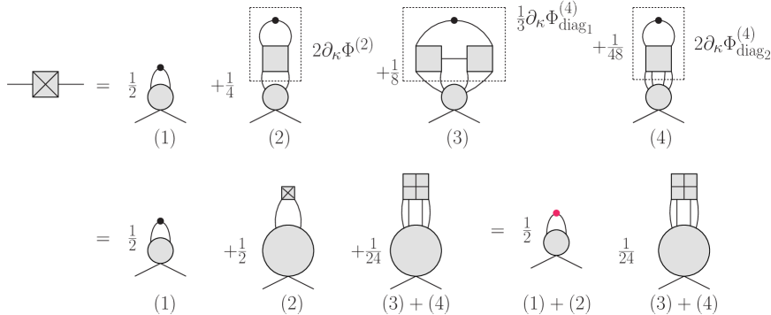
Figure 15: The diagrams produced when the BS equation in figure 10 is substituted into the tadpole diagram in the first line of figure 2. In the second line we regroup the graphs by re-substituting the RG equations and using figure 1. The numbers under each diagram indicate the pieces of figure 10 that contributed.

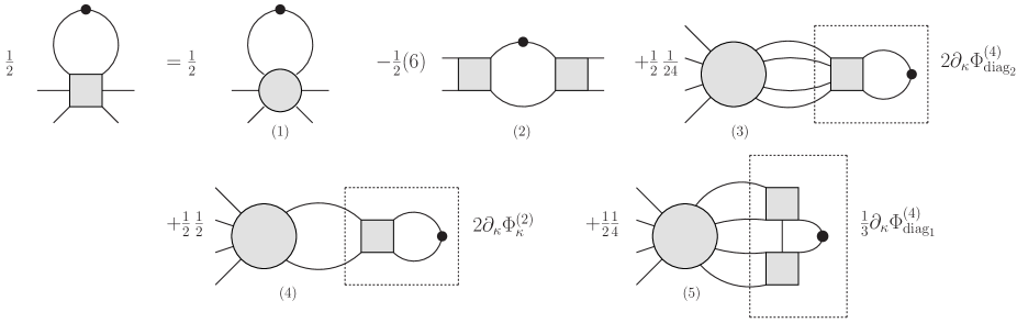
Figure 16: The result of substituting the 6-point vertex in figure 11 into the tadpole diagram in the second line of figure 2.

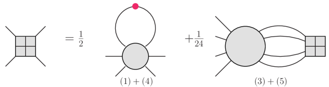
Figure 17: The second RG equation truncated with the BS equation in figure 11. The numbers under the diagrams correspond to the pieces of figure 16 that were combined. The diagram labelled (2) in figure 16 cancels the bubble graph in figure 2.

Now we compare our results for $\partial_{\kappa}\Phi_{\kappa}^{(2)}$ and $\partial_{\kappa}\Phi_{\kappa}^{(4)}$ in figures 15 and 17 with the derivatives $\partial_{\kappa}\Sigma_{\kappa}$ and $\partial_{\kappa}V_{\kappa}$ of the 2- and 4-point functions obtained from the 4PI equations of motion and extended to the deformed theory. Note that the vertex $V_{\kappa}$ depends on the flow parameter $\kappa$ only indirectly through the fact that the equation of motion for the 4-point function is coupled to the equation of motion for the 2-point function, which is evaluated at $G=G_{\kappa}$ after the functional derivatives are taken.

In the 4PI theory equation (31) becomes:

$$\partial_{\kappa}(\Sigma_{ij})_{\kappa} =2\partial_{\kappa}(G_{kl})_{\kappa}\frac{\delta^{2}\Phi}{\delta G_{kl}\delta G_{ij}}\bigg{|}_{G_{\kappa}}$$ (47)

$$+2\partial_{\kappa}(V_{klrs})_{\kappa}(G_{ka})_{\kappa}(G_{lb})_{\kappa}(G_{rc})_{\kappa}(G_{sd})_{\kappa}\;G^{-1}_{aa^{\prime}}G^{-1}_{bb^{\prime}}G^{-1}_{cc^{\prime}}G^{-1}_{dd^{\prime}}\frac{\delta^{2}\Phi}{\delta V_{a^{\prime}b^{\prime}c^{\prime}d^{\prime}}\delta G_{ij}}\bigg{|}_{G_{\kappa}}$$

$$=\frac{1}{2}\partial_{\kappa}(G_{kl})_{\kappa}(\Lambda_{ijkl})_{\kappa}+\frac{1}{24}\,\partial_{\kappa}(V_{klrs})_{\kappa}(G_{ka})_{\kappa}(G_{lb})_{\kappa}(G_{rc})_{\kappa}(G_{sd})_{\kappa}(\Lambda_{\kappa})_{abcdij}\,.$$

Equation (47) is precisely the result that is shown in the last line of figure 15 if we identify $V_{\kappa}=\Phi^{(4)}_{\kappa}$, which means we have obtained the equation

$$\partial_{\kappa}\Phi_{\kappa}^{(2)}(p)=\partial_{\kappa}\Sigma_{\kappa}(p)\,,$$ (48)

at the level of the 4PI effective action.

For the 4-point function we have:

$$\partial_{\kappa}(V_{xywz})_{\kappa} =4!\partial_{\kappa}\bigg{[}G^{-1}_{xx^{\prime}}G^{-1}_{yy^{\prime}}G^{-1}_{ww^{\prime}}G^{-1}_{zz^{\prime}}\frac{\partial^{2}\hat{\Phi}}{\delta V_{x^{\prime}y^{\prime}w^{\prime}z^{\prime}}}\bigg{]}_{G=G_{\kappa}}$$ (49)

$$=4!\partial_{\kappa}(G_{ab})_{\kappa}\bigg{[}\frac{\delta}{\delta G_{ab}}\bigg{(}G^{-1}_{xx^{\prime}}G^{-1}_{yy^{\prime}}G^{-1}_{ww^{\prime}}G^{-1}_{zz^{\prime}}\;\frac{\partial\hat{\Phi}}{\delta V_{x^{\prime}y^{\prime}w^{\prime}z^{\prime}}}\bigg{)}\bigg{]}_{G=G_{\kappa}}$$

$$~{}~{}~{}~{}~{}~{}+\partial_{\kappa}(V_{abcd})_{\kappa}\bigg{[}\frac{\delta}{\delta V_{abcd}}\bigg{(}G^{-1}_{xx^{\prime}}G^{-1}_{yy^{\prime}}G^{-1}_{ww^{\prime}}G^{-1}_{zz^{\prime}}\;\frac{\partial\hat{\Phi}}{\delta V_{xywz}}\bigg{)}\bigg{]}_{G=G_{\kappa}}$$

$$=\frac{1}{2}\partial_{\kappa}(G_{ab})_{\kappa}(\Lambda_{abxywz})_{\kappa}+\frac{1}{4!}\partial_{\kappa}(V_{abcd})_{\kappa}(G_{ax})_{\kappa}(G_{by})_{\kappa}(G_{cw})_{\kappa}(G_{dz})_{\kappa}(\Lambda_{abcdxywz})_{\kappa}\,.$$

The hat indicates that the basketball diagram has been removed from the effective action (since this is the diagram that produces the left side in the V equation of motion in figure 5 - see the discussion under equation (20)). The basketball diagram does not contribute to either the 6-point or 8-point kernel (it produces $\Lambda_{abcdxywz}^{\rm disco}$). There are no contributions from the functional derivative with respect to $G$ acting on the inverse propagators because the sum of these terms gives zero using the $V$ equation of motion. Equation (49) is exactly the equation shown in figure 17 if we use $V_{\kappa}=\Phi^{(4)}_{\kappa}$. Thus we have obtained:

$$\partial_{\kappa}\Phi_{\kappa}^{(4)}(p_{1},p_{2},p_{3},-p_{1}-p_{2}-p_{3})=\partial_{\kappa}V_{\kappa}(p_{1},p_{2},p_{3},-p_{1}-p_{2}-p_{3})\,,$$ (50)

which is the generalization of equation (46) to non-diagonal momenta.

Equations (48) and (50) show that the RG equations for the 2- and 4-point functions are total derivatives whose integrals can be written as the 4PI equations of motion.

VIII Conclusions

In this paper we have studied the connection between two different formalisms that are commonly used to study non-perturbative systems: the exact renormalization group and $n$-particle irreducible effective theories. We have derived Bethe-Salpeter type integral equations that can be used to truncate the RG flow equations, and shown that the resulting flow equations for the 2- and 4-point functions are total derivatives whose integrals give the $n$PI eom’s. Since the full hierarchy of RG flow equations are obtained using a single bi-local source term, this result is surprising and suggests that a BS truncation at arbitrary orders produces equations whose integrals gives the $n$PI eom’s. This establishes a direct connection between two non-perturbative methods. It also means that the truncation of the RG equations at any level of the hierarchy can be systematically extended by adding more and more skeleton diagrams to the effective action. For the $n$PI formalism, there might be a practical advantage in reformulating the integral equations as flow equations, because initial value problems are usually easier to solve than non-linear integral equations.

Appendix A Derivation of the BS equation for the diagonal 6-point vertex from the 2PI effective action

In this appendix we give some details of the derivation of the result in figure 8. Substituting equations (24), (25), (36) and (39) into (35) one finds immediately that all terms that contain a factor $\delta_{ij}$ cancel exactly. There are 10 remaining terms, which are shown in figure 18. The 6-point boxes in this figure are amputated vertex functions, which is indicated by the letter ‘$A$’ inside each box.

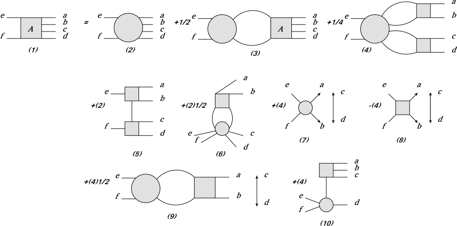
Figure 18: The diagonal 6-point vertex function in terms of amputated vertices.

The diagrams in parts (7), (8) and (9) of the figure contain disconnected contributions, but one immediately sees that they cancel using the lower-order BS equation in equation (27). Parts (1) and (3) of the figure can be written in terms of proper vertex functions using:

$$V^{\rm amputated}_{abcdef} =V_{abcdef}+G_{z_{7}z_{8}}V_{abcz_{8}}V_{defz_{7}}+G_{z_{7}z_{8}}V_{abdz_{8}}V_{cefz_{7}}+G_{z_{7}z_{8}}V_{acdz_{8}}V_{befz_{7}}+G_{z_{7}z_{8}}V_{aefz_{7}}V_{bcdz_{8}}$$ (51)

$$+G_{z_{7}z_{8}}V_{abez_{8}}V_{cdfz_{7}}+G_{z_{7}z_{8}}V_{acez_{8}}V_{bdfz_{7}}+G_{z_{7}z_{8}}V_{adfz_{7}}V_{bcez_{8}}+G_{z_{7}z_{8}}V_{adez_{8}}V_{bcfz_{7}}$$

$$+G_{z_{7}z_{8}}V_{acfz_{7}}V_{bdez_{8}}+G_{z_{7}z_{8}}V_{abfz_{7}}V_{cdez_{8}}\,,$$

$$=V_{abcdef}+(10)G_{z_{7}z_{8}}V_{abcz_{8}}V_{defz_{7}}\,.$$

The results are shown in figures 19 and 20. One can see immediately that (1C) cancels (5), and (1D) and (3D) cancel (10) when we use the BS equation for the 4-vertex in (27) in the lower vertex in (10). The survivors are shown in figure 8.

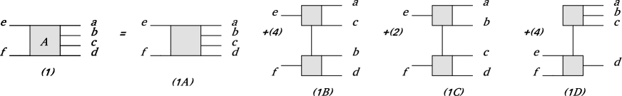
Figure 19: The diagram in part (1) of figure 18 in terms of proper vertices.

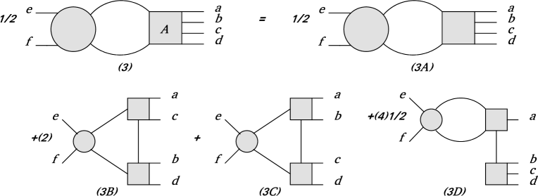
Figure 20: The diagram in part (3) of figure 18 in terms of proper vertices.

Appendix B Derivation of the functional derivative $\delta V/\delta R$

In this appendix we calculate $\delta V_{xywz}/\delta R_{ab}$ using the same technique as in sections V.1 and VI.2. In the symmetric theory we have:

$$\frac{\delta}{\delta R_{ab}}V_{xywz}=\frac{\delta}{\delta R_{ab}}\bigg{(}G^{-1}_{xx^{\prime}}G^{-1}_{xx^{\prime}}G^{-1}_{xx^{\prime}}G^{-1}_{xx^{\prime}}V^{c}_{x^{\prime}y^{\prime}w^{\prime}z^{\prime}}\bigg{)}\,.$$ (52)

We separate the contributions from the derivative acting on the inverse propagators and the connected vertex function. If the derivative acts only on the vertex function we have:

$$G^{-1}_{xx^{\prime}}G^{-1}_{yy^{\prime}}G^{-1}_{ww^{\prime}}G^{-1}_{zz^{\prime}}\frac{\delta}{\delta R_{ab}}V^{c}_{x^{\prime}y^{\prime}w^{\prime}z^{\prime}}$$ (53)

$$=G^{-1}_{xx^{\prime}}G^{-1}_{yy^{\prime}}G^{-1}_{ww^{\prime}}G^{-1}_{zz^{\prime}}\frac{\delta}{\delta R_{ab}}\big{(}\langle\varphi_{x^{\prime}}\varphi_{y^{\prime}}\varphi_{w^{\prime}}\varphi_{z^{\prime}}\rangle-\langle\varphi_{x^{\prime}}\varphi_{y^{\prime}}\rangle\langle\varphi_{w^{\prime}}\varphi_{z^{\prime}}\rangle-\langle\varphi_{x^{\prime}}\varphi_{w^{\prime}}\rangle\langle\varphi_{y^{\prime}}\varphi_{z^{\prime}}\rangle-\langle\varphi_{x^{\prime}}\varphi_{z^{\prime}}\rangle\langle\varphi_{y^{\prime}}\varphi_{w^{\prime}}\rangle\big{)}\,,$$

$$=\frac{i}{2}G^{-1}_{xx^{\prime}}G^{-1}_{yy^{\prime}}G^{-1}_{ww^{\prime}}G^{-1}_{zz^{\prime}}\bigg{(}\langle\varphi_{x^{\prime}}\varphi_{y^{\prime}}\varphi_{w^{\prime}}\varphi_{z^{\prime}}\varphi_{a}\varphi_{b}\rangle-G_{ab}\langle\varphi_{x^{\prime}}\varphi_{y^{\prime}}\varphi_{w^{\prime}}\varphi_{z^{\prime}}\rangle-(6)G_{x^{\prime}y^{\prime}}\langle\varphi_{a}\varphi_{b}\varphi_{w^{\prime}}\varphi_{z^{\prime}}\rangle\$$

$$~{}~{}~{}~{}~{}~{}~{}~{}~{}~{}~{}~{}~{}~{}~{}~{}~{}~{}~{}+2(3)G_{ab}G_{x^{\prime}y^{\prime}}G_{wz}\bigg{)}\,,$$

$$=\frac{i}{2}\bigg{(}(8)G_{az_{1}}\delta_{bz}V_{wxyz_{1}}+(4)G_{z_{3}z_{4}}G_{az_{1}}G_{bz_{2}}V_{xz_{1}z_{2}z_{3}}V_{wyzz_{4}}+(6)G_{z_{3}z_{4}}G_{az_{1}}G_{bz_{2}}V_{xzz_{2}z_{3}}V_{wyz_{1}z_{4}}$$

$$~{}~{}~{}~{}~{}~{}+G_{az_{1}}G_{bz_{2}}V_{wxyzz_{1}z_{2}}\bigg{)}\,.$$

Now we consider the contribution obtained when the derivative acts only on the inverse propagators. To differentiate the inverse propagators we use:

$$\frac{\delta G^{-1}_{ij}}{\delta R_{ab}} =\frac{\delta G^{-1}_{ij}}{\delta G_{mn}}\frac{\delta G_{mn}}{\delta R_{ab}}\,,$$ (54)

with the result for $\delta G_{mn}/\delta R_{ab}$ given in equation (25) and the derivative of the inverse propagator given by:

$$-2\frac{\delta G^{-1}_{ij}}{\delta G_{mn}}=G^{-1}_{im}G^{-1}_{jn}+G^{-1}_{in}G^{-1}_{jm}\,.$$ (55)

Using equations (25), (54) and (55) we obtain:

$$V^{c}_{x^{\prime}y^{\prime}w^{\prime}z^{\prime}}\frac{\delta}{\delta R_{ab}}\bigg{(}G^{-1}_{xx^{\prime}}G^{-1}_{xx^{\prime}}G^{-1}_{xx^{\prime}}G^{-1}_{xx^{\prime}}\bigg{)}=-\frac{i}{2}\bigg{(}(8)G_{az_{1}}\delta_{bz}V_{wxyz_{1}}+(4)G_{z_{3}z_{4}}G_{az_{1}}G_{bz_{2}}V_{xz_{1}z_{2}z_{3}}V_{wyzz_{4}}\bigg{)}\,.$$

$$\,.$$ (56)

Substituting the results in equations (53) and (B) into (52) we obtain:

$$\frac{\delta}{\delta R_{ab}}V_{xywz}=\frac{i}{2}G_{az_{1}}G_{bz_{2}}\bigg{(}V_{wxyzz_{1}z_{2}}+(6)G_{z_{3}z_{4}}V_{xzz_{2}z_{3}}V_{wyz_{1}z_{4}}\bigg{)}\,.$$ (57)

References

- (1) J.M. Cornwall, R. Jackiw, and E. Tomboulis, Phys. Rev. D 10, 2428 (1974).
- (2) R.E. Norton and J.M. Cornwall, Annals of Physics 91, 106 (1975).
- (3) C. Wetterich, Phys. Lett., B301, 90 (1993).
- (4) U. Ellwanger, Z. Phys. C58, 619 (1993).
- (5) N. Tetradis and C. Wetterich, Nucl. Phys. B 422, 541 (1994).
- (6) T.R. Morris, Phys. Lett. B329, 241 (1994).
- (7) J. P. Blaizot, E. Iancu, and A. Rebhan, Phys. Rev. Lett. 83, 2906 (1999), arXiv:hep-ph/9906340; Phys. Rev. D 63, 065003 (2001), arXiv:hep-ph/0005003.
- (8) J. Berges, Sz. Borsányi, U. Reinosa, and J. Serreau, Phys. Rev. D 71, 105004 (2005), arXiv:hep-ph/0409123.
- (9) J. Berges and J. Cox, Phys. Lett. B 517, 369 (2001), arXiv:hep-ph/0006160; J. Berges, Nucl. Phys. A 699, 847 (2002), arXiv:hep-ph/0105311; G. Aarts and J. Berges, Phys. Rev. Lett. 88, 041603 (2002), arXiv:hep-ph/0107129; G. Aarts, D. Ahrensmeier, R. Baier, J. Berges, and J. Serreau, Phys. Rev. D 66, 045008 (2002), arXiv:hep-ph/0201308.
- (10) G. Aarts and J. M. Martínez Resco, JHEP 02, 061 (2004).
- (11) M.E. Carrington and E. Kovalchuk, Phys.Rev. D77, 025015 (2008).
- (12) M.E. Carrington and E. Kovalchuk, Phys. Rev. D80, 085013 (2009).
- (13) M.E. Carrington and E. Kovalchuk, Phys. Rev. D81, 065017 (2010).
- (14) T. R. Morris, Prog. Theor. Phys. Suppl. 131, 395 (1998); Int. J. Mod. Phys. B12 (1998) 1343-1354;
- (15) C. Bagnuls and C. Bervillier, Phys. Rept. 348, 91 (2001).
- (16) J. Berges, N. Tetradis and C. Wetterich, Phys. Rept. 363, 223 (2002).
- (17) J. M. Pawlowski, Annals Phys. 322 (2007) 2831.
- (18) B. Delamotte, cond-mat/0702365.
- (19) O. J. Rosten, arXiv:1003.1366.
- (20) Jean-Paul Blaizot, Phil. Trans. R. Soc. A 369, 2735 (2011).
- (21) Jean-Paul Blaizot, Jan M. Pawlowski, Urko Reinosa, Phys. Lett. B696, 523 (2011).
- (22) M. E. Carrington, Wei-Jie Fu - arXiv:1202.3165
- (23) M. E. Carrington, Wei-Jie Fu - in progress
- (24) D. Binosi and L. Theussl, Comput. Phys. Commun. 161, 76 (2004), arXiv:hep-ph/0309015.
- (25) M.E. Carrington, Eur. Phys. J. C35, 83 (2004).
- (26) J. Berges, Phys. Rev. D 70, 105010 (2004).
- (27) H. van Hees and J. Knoll, Phys. Rev. D 65, 025010 (2002); ibid. 105005 (2002).
- (28) A. Arrizabalaga and J. Smit, Phys. Rev. D66, 065014 (2002).
- (29) M.E. Carrington, G. Kunstatter and H. Zaraket, Eur. Phys. J. C42, 253 (2005).
- (30) D. Binosi and J. Papavassiliou, Physics Reports, 479, 1 (2009).
- (31) U. Reinosa and J. Serreau, Annals Phys. 325, 969 (2010).