Occurrence conditions for two-dimensional Borromean systems

Abstract

We search for Borromean three-body systems of identical bosons in two dimensional geometry, i.e. we search for bound three-boson system without bound two-body subsystems. Unlike three spatial dimensions, in two-dimensional geometry the two- and three-body thresholds often coincide ruling out Borromean systems. We show that Borromean states can only appear for potentials with substantial attractive and repulsive parts. Borromean states are most easily found when a barrier is present outside an attractive pocket. Extensive numerical search did not reveal Borromean states for potentials without an outside barrier. We outline possible experimental setups to observe Borromean systems in two spatial dimensions.

1 Introduction

In quantum mechanics two particles in three spatial dimensions (3D) can attract each other without forming a bound state. However adding a third particle can make a three-body system bound. Such bound three-body structures, where each pair of particles is unbound, are called Borromean states. They turn out to be rather abundant in subatomic physics where many examples are found and studied, see e.g. zhukov1993 ; riisager2012 . Those examples raised the question about properties of the potentials that determine the possibility for Borromean binding. One can trace this discussion for three-dimensional geometry in numerous papers, e.g. richard1994 ; richard2000 . It turns out that in 3D finite range potentials of the form $gV(r)$ most likely have a region of the parameter $g$ where three, but not two particles are bound.

In two spatial dimensions (2D), however, this question is not well-established. The result has to be different, because two-body binding is easier to achieve in 2D than in 3D. This is shown already for two particles with $gV<0$. Such potentials support two- and three-body bound states even when $g\rightarrow 0$ landau1977 . The thresholds for binding of two and three-body systems are identical and Borromean structures cannot exist. Moreover, numerical investigations in momentum space tjon1980 ; frederico1988 and coordinate space cabral1979 ; lim1980 ; nielsen1999 ; hammer2004 ; blume2005 ; hammer2011 revealed that in 2D some other classes of potentials have no Borromean states.

Previous investigations also show, that it is not entirely impossible to have Borromean systems in 2D. However, to the best of our knowledge, only one example of an appropriate two-body potential can be found in the literature nielsen1999 . The purpose of this report is to identify conditions for the two-body potentials that can produce Borromean systems of three identical bosons in two dimensions. We believe that using advanced experimental techniques it is possible to create setups where these conditions are satisfied. This introduces structures with new few- and many- body properties. This investigation also puts limitations for a zero-range formalism that is used widely to describe few-body dynamics in 2D kart2006 ; bel2011 ; bel2012 ; bel2013 . This formalism is a powerful tool which has been proven to give correct results for weakly-bound systems in 2D that have identical three and two body thresholds. However it can not describe Borromean states where finite-range techniques have to be used.

We believe that this investigation is timely and important. First, because the experimental techniques in cold atomic gases are rapidly improving in 3D and are currently being adjusted to 2D. Second, a Borromean system has three particles which strongly suggests that traditional many-body correlations built on two-body properties now may turn out to be completely different if three particles are considered as building blocks. Our results provide guidence to the tuning of the potentials in order to achieve new many-body structures.

In this report we briefly discuss conditions for two-body binding in section II. We search for characteristic properties, e.g. shape of the potential $V$ and strength $g$, which allow binding of three but not of two particles in section III. We outline experimental setups to observe Borromean states in section IV. Finally, in section V we briefly summarize and conclude.

2 Two-body problem in two dimensions

According to the definition Borromean states, if they exist, appear for two-body potentials at the edge of two-body binding. An additional particle then provides the glue to form a three-body bound state. We therefore first must establish the criteria for a two-body potential to support a bound state first_footnote . This is known in the limit of weak potentials, $g\rightarrow 0$, where the net volume, $g\int Vr\mathrm{d}r$, simply has to be non-positive. However, the existence of bound states for stronger potentials is not solely determined by the net volume. Thus we reformulate the two-body problem with the aim of extracting suitable criteria for binding. The qualitative behavior is supplemented by a full quantitative analysis for simple potentials.

2.1 General properties

The radial Schrödinger equation for two particles in 2D is

$$\frac{\hbar^{2}}{2\mu}\bigg{(}-\frac{1}{r}\frac{\partial}{\partial r}r\frac{\partial}{\partial r}+\ \frac{M^{2}}{r^{2}}\bigg{)}\phi_{M}=(E_{2}-gV)\phi_{M}\;,$$ (1)

where $r$ is the relative coordinate, $E_{2}$ the two-body energy, $gV(r)$ the potential, $\mu$ the reduced mass, and $M=0,1,2,...$ is the angular quantum number, $\phi_{M}$ the wave function of the relative motion. For spherical potentials $M$ is conserved and $M=0$ therefore characterizes the ground state for identical bosons. We shall in the following only consider $M=0$ and omit any related index.

We demand the wave function, $\phi(k,r)$, to be regular in zero, through $\phi(k,r=0)=1$, where $k$ is the wave number given by $E_{2}=\hbar^{2}k^{2}/(2\mu)$. The condition for a bound state can then be written as vol10 ; vol11

$$1+\frac{2g\mu}{\hbar^{2}}\frac{i\pi}{2}\int_{0}^{\infty}\mathrm{d}rr\phi(k,r)V(r)H_{0}^{(1)}(kr)=0\;,$$ (2)

where $H_{0}^{(1)}$ is the first Hankel function of order zero. The solutions correspond to bound states with $k=i|k|$. We focus on the weak binding limit where $k$ approaches zero and eq. (2) reduces to

$$1+\frac{2g\mu}{\hbar^{2}}\int_{0}^{\infty}\mathrm{d}rr\phi(0,r)V(r)\big{(}i\frac{\pi}{2}-\ln(\frac{kr}{2}e^{\gamma})\big{)}=0\;,$$ (3)

where $\gamma$ is Euler’s constant and the regular zero energy solution to eq. (1) is

$$\phi(0,r)=1+\frac{2g\mu}{\hbar^{2}}\int_{0}^{r}\mathrm{d}ss\ln{(r/s)}V(s)\phi(0,s)\;.$$ (4)

Then eq. (3) can only be fulfilled for small $k$ when

$$g\int_{0}^{\infty}\mathrm{d}rr\phi(0,r)V(r)=0\;.$$ (5)

Eqs. (3) and (4) define appearence of the bound state in 2D. This result might also be obtained using the Jost function formalism, see gibson1986 .

From eq. (1) we get immediately

$$g\int_{0}^{R}\mathrm{d}rr\phi(0,r)V(r)=\frac{\hbar^{2}}{2\mu}\bigg{(}r\frac{\partial}{\partial r}\phi(0,r)\bigg{)}\bigg{|}_{r=R}=0\;,$$ (6)

where the vanishing result is obtained for finite-range potentials where $V(r>R)=0$. Thus the slope of the zero-energy wave function is zero at $r=R$.

It is obvious that for purely attractive potentials, $gV<0$, the condition from eq. (5) can be achieved only for $g=0$. This is a consequence of the fact that purely attractive potentials always provide at least one two-body bound state in 2D landau1977 . In this case the thresholds for binding of two and three-body systems has to coincide hence Borromean states are ruled out nielsen1999 .

It gives us the first necessary condition for Borromean binding: the potential, $gV$, has to contain both positive and negative parts. We shall proceed by defining shapes $V_{\pm}$ and dimensionless strengths $\lambda_{\pm}>0$ of the positive and negative parts. The total potential is then given by $gV(r)=\lambda_{+}V_{+}+\lambda_{-}V_{-}$. Binding is subsequently achieved by sufficient increase of $\lambda_{-}$, and binding is reduced by increase of $\lambda_{+}$. We define the critical repulsive interaction, $\lambda_{+}^{(cr)}(\lambda_{-})$, through eq. (5) by

$$\int_{0}^{\infty}\mathrm{d}rr\phi(0,r)(\lambda_{+}^{cr}V_{+}+\lambda_{-}V_{-})=0\;.$$ (7)

This implies that a Borromean system can only appear when $\lambda_{+}$ is larger than $\lambda_{+}^{cr}$, since two particles are unbound in this regime. Hence a Borromean system for given $\lambda_{-}$ might be found in an interval where $\lambda_{+}$ is larger than $\lambda_{+}^{cr}$, although perhaps an interval of very limited extension. The solution of eq. (4) and the definition in eq. (7) then provide crucial information about the most likely region for occurrence of Borromean systems.

Let us use eq. (7) for potentials, where knowledge of the wave function is not needed. First we show the well established result that any weak potential with negative or zero net volume has at least one bound state landau1977 ; vol10 ; simon1976 . When the attractive part is very weak we can appoximate the wave function in eq. (4) by the first term. This gives

$$\lambda_{+}^{cr}=-\lambda_{-}\frac{\int\mathrm{d}rrV_{-}(r)}{\int\mathrm{d}rrV_{+}(r)}+O(e^{-\frac{c}{\lambda_{-}^{2}}}).$$ (8)

Then from eq. (7) we see that when $\lambda_{+}\leq\lambda_{+}^{cr}$ the net volume is less than $O(e^{-\frac{c}{\lambda_{-}^{2}}})\ll\lambda_{-}$ and at least one bound state is present, whereas the system is unbound for $\lambda_{+}>\lambda_{+}^{cr}$ where the net volume is positive. This result leads us to a second necessary condition for a Borromean system, that is $g\int Vr\mathrm{d}r>0$, as only those potentials have a region of $g$ without two-body states.Second, we consider the two delta-shell potentials, $gV=\hbar^{2}/(2\mu d^{2})\big{(}\lambda_{+}\delta(r/c-1)-\lambda_{-}\delta(r/d-1))$, which is infinitely large for a given radial distance and zero otherwise. In the limit when $c\rightarrow d$ we immediately conclude from eq. (7) and continuity of the wave function that $\lambda_{+}^{cr}=-\lambda_{-}$.

Other potentials localize the wave function in the attractive region, which increases $\int\mathrm{d}rrV_{-}(r)\phi(0,r)$ and decreases $\int\mathrm{d}rrV_{+}(r)\phi(0,r)$. Eq. (7) then strongly suggests a steep increase of $\frac{\mathrm{d}\lambda_{+}^{cr}}{\mathrm{d}\lambda_{-}}$ at a given sufficiently large value of $\lambda_{-}$. Or, in another words, if the potential is of finite range then for $\lambda_{+}^{cr}\rightarrow\infty$ a finite $\lambda_{-}^{cr}$ exists that will bind the two-body system.

2.2 Square well with barrier or core

The threshold conditions are not easily derived for arbitrary potentials with sizable attraction and repulsion. However, the general equations, eqs. (7) and (4), are directly applicable for simple potentials where zero-energy wave functions are known. From properly selected potentials we can then extract correct qualitative properties for more general potentials. We choose to study a solvable model containing all the crucial features, that is

$$V=\lambda_{-}V_{-}+\lambda_{+}V_{+}=\left\{\begin{array}[]{ll}-\frac{\lambda_{-}\hbar^{2}}{2\mu R_{s}^{2}}&r\leq R_{s}\\ \frac{\lambda_{+}\hbar^{2}}{2\mu R_{s}^{2}}&R_{s}<r\leq R_{l}\\ 0&r>R_{l}\;,\end{array}\right.$$ (12)

where $R_{s}$ and $R_{l}$ are positive radii. This potential is useful for describing qualitative features of more general potentials, see e.g.  jeremy2010 . The zero-energy solution then has the form

$$\phi(0,r)=\left\{\begin{array}[]{ll}AJ_{0}(k_{1}r)&\;r\leq R_{s}\\ BI_{0}(k_{2}r)+CK_{0}(k_{2}r)&\;R_{s}<r\leq R_{l}\\ DK_{0}(k_{3}r)&\;r>R_{l}\;,\end{array}\right.$$ (13)

where $k_{1}=\sqrt{\lambda}_{-}/R_{s}$, $k_{2}=\sqrt{\lambda}_{+}/R_{s}$, $k_{3}\rightarrow 0$, $J_{0},I_{0},K_{0}$ are Bessel functions with the usual definitions abram64 , and the constants $B,C,D$ are defined through $A$ by matching at the points $r=R_{s}$ and $R_{l}$. One of these equations is the quantization condition providing the energy $E$. For $E=0$ we use instead eq. (7), which by use of $xZ_{0}(x)=\frac{\mathrm{d}}{\mathrm{d}x}xZ_{1}(x),Z_{i}=I_{i},Y_{i},J_{i}$, $xK_{0}(x)=-\frac{\mathrm{d}}{\mathrm{d}x}xK_{1}(x)$ and the wave function in eq. (13) can be integrated to give

$$aI_{1}(k_{2}R_{l})=bK_{1}(k_{2}R_{l}),\;$$ (14)

where the constants $a$ and $b$ are defined by

$$a = k_{2}J_{0}(k_{1}R_{s})K_{1}(k_{2}R_{s})-k_{1}J_{1}(k_{1}R_{s})K_{0}(k_{2}R_{s}),$$

$$b = k_{2}J_{0}(k_{1}R_{s})I_{1}(k_{2}R_{s})+k_{1}J_{1}(k_{1}R_{s})I_{0}(k_{2}R_{s}).$$ (15)

The derivation of eqs. (14) and (15) employed the bound state boundary condition and the relations $J_{0}(x)Y_{1}(x)-J_{1}(x)Y_{0}(x)=-\frac{2}{\pi x}$ and $I_{0}(x)K_{1}(x)+I_{1}(x)K_{0}(x)=\frac{1}{x}$.

First we start with overall weak potentials, that is $k_{2}R_{s}\rightarrow 0$ and $k_{1}R_{s}\rightarrow 0$. Then the properties of the Bessel functions give $a\rightarrow 1/R_{s}$ and $b\rightarrow R_{s}(k_{1}^{2}+k_{2}^{2})/2$. Using that $J_{1}(x)\approx x/2,K_{1}(x)\approx 1/x$ we find that eq. (14) is equivalent to $\int Vr\mathrm{d}r=0$, and coinciding with eq. (8).

The other limit of a sizable barrier where $k_{2}R_{s}\gg 1$ can also be found analytically. After some manipulations using properties of the Bessel functions, we conclude that Eq. (14) can be approximated by

$$k_{2}R_{s}J_{0}(k_{1}R_{s})-k_{1}R_{s}J_{1}(k_{1}R_{s})=0\;,$$ (16)

where we assumed that $R_{l}\neq R_{s}$. Thus, the solution has to be near the nodes of the Bessel function, since $J_{0}(k_{1}R_{s})=k_{1}R_{s}J_{1}(k_{1}R_{s})/(k_{2}R_{s})\rightarrow 0$. Continuity of the wave function at $r=R_{s}$ combined with the exponential decrease by penetrating into a barrier then in turn implies that the wave function must be severely diminishing with increasing barrier.

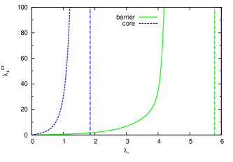
Figure 1: The critical strength, $\lambda_{+}^{cr}$, on the positive part of the potential as function of the strength, $\lambda_{-}$, on the negative part. We use $R_{s}/R_{l}=1/2$. The two curves are for the square well with a barrier (solid green), eq. (14), and the inverted with a core and no outer barrier (dashed blue), eq. (21). The vertical dot-dashed lines are the corresponding asymptotic values, $\lambda_{-}^{cr}$.

The critical value, $\lambda_{+}^{cr}$, are shown in Fig. 1 as function of $\lambda_{-}$, see eq. (14). The behavior is typical and thus characterizes also the behavior for less schematic potentials. The linear behavior for weak potentials (small $\lambda_{-}$) is as predicted in eq. (8). As $\lambda_{-}$ increases the critical repulsion rises steeply and at some point, $\lambda_{-}^{cr}$, it cannot compensate to avoid a bound state. Larger attraction, $\lambda_{-}>\lambda_{-}^{cr}$, always provides two-body binding.

The potential in eq. (12) could as well be understood with positive and negative parts interchanged.

$$V=\lambda_{-}V_{-}+\lambda_{+}V_{+}=\left\{\begin{array}[]{ll}\frac{\lambda_{+}\hbar^{2}}{2\mu R_{s}^{2}}&r\leq R_{s}\\ -\frac{\lambda_{-}\hbar^{2}}{2\mu R_{s}^{2}}&R_{s}<r\leq R_{l}\\ 0&r>R_{l}\;,\end{array}\right.$$ (20)

Then the corresponding condition in eq. (14) has to be modified as achieved most easily by analytic continuation. This implies the use of $k_{1}=\sqrt{\lambda_{+}}/R_{s},k_{2}=\sqrt{\lambda_{-}}/R_{s}$, resulting in

$$\tilde{a}J_{1}(k_{2}R_{l})=\tilde{b}Y_{1}(k_{2}R_{l})\;,$$ (21)

where the constants correspondingly have to be changed to

$$\tilde{a} = k_{2}I_{0}(k_{1}R_{s})Y_{1}(k_{2}R_{s})+k_{1}I_{1}(k_{1}R_{s})Y_{0}(k_{2}R_{s}),$$

$$\tilde{b} = k_{2}I_{0}(k_{1}R_{s})J_{1}(k_{2}R_{s})+k_{1}I_{1}(k_{1}R_{s})J_{0}(k_{2}R_{s}).$$ (22)

For weak potentials we again find $\tilde{a}\rightarrow 1/R_{s},\tilde{b}\rightarrow(k_{2}^{2}R_{s}+k_{1}^{2}R_{s})/2$, which as before leads to the condition for binding with zero net volume.

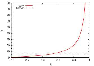
Figure 2: The dimensionless volume, $h$, of the attractive part as function of the ratio, $s=R_{s}/R_{l}$, of inner and outer radius for the square well potential with a repulsive inner core, see eq. (23). The horizontal dashed line is the volume needed to bind two particles when an outer barrier is present, see eq. (16).

However, these potentials of finite size with $k_{1}R_{s}\gg 1$ behave qualitatively different from the potential in eq. (12). In this limit it is again possible to reduce eq. (21) to give

$$J_{0}(k_{2}R_{s})Y_{1}(k_{2}R_{l})-J_{1}(k_{2}R_{l})Y_{0}(k_{2}R_{s})=0.$$ (23)

This equation provides the boundary condition for a wave function which is zero at $r=R_{s}$ and has zero derivative at $r=R_{l}$. This condition for binding by an attractive square well then depends on both $k_{2}R_{s}$ and $k_{2}R_{l}$. These two parameters can be expressed in terms of the dimensionless measure of the attractive volume, i.e. $h=k_{2}^{2}(R_{l}^{2}-R_{s}^{2})$, and the ratio between the two radii $s=k_{2}R_{s}/(k_{2}R_{l})<1$, that is $k_{2}^{2}R_{l}^{2}=h/(1-s^{2})$ and $k_{2}^{2}R_{s}^{2}=hs^{2}/(1-s^{2})$. Expressed by $h$ and $s$, eq. (23) determines $h$ as function of $s$ as shown in Fig. 2. For $s\rightarrow 1$, $h\sim\frac{1}{1-s}$ and for small values of $s$: $h\sim-1/\ln s$. We note the continuous approach to the $s=0$ limit which corresponds to the binding in an overall attractive potential where only infinitesimal strength or volume is necessary. The other limit of $s=1$ exhibits that the potential must be infinitely deep when the two radii approach each other at a finite value. This variation is completely different from the condition of binding for the potential from eq. (12) where the volume for deep potentials is independent of the barrier dimension. We also solve eq. (21) for given ratio $R_{l}/R_{s}$ and exhibit $\lambda_{+}^{cr}$ as function of $\lambda_{-}$ in Fig. 1. Again we find slow convergence towards the asymptotic value obtained from eq. (23).

In 1D we consider potentials given by eqs. (12) and (20) for $x>0$ and infinite wall for $x<0$. We write then, instead of eq. (16), $k_{1}R_{s}=\pi$, where only $k_{1}R_{s}$ is present and eq.(23) is replaced by $k_{2}(R_{l}-R_{s})=\pi/2$, where only the difference $R_{l}-R_{s}$ appears due to translational invariance landau1977 . In 3D we get a radial equation which is the same as in 1D. Moreover we also have the same boundary conditions, because we assume that 1D potentials have an infinite wall for negative $x$. Thus, in 3D we get the threshold conditions,$k_{1}R_{s}=\pi$ and $k_{2}(R_{l}-R_{s})=\pi/2$ for potentials from eqs. (12) and (20) respectively.

So far we can conclude that only potentials with positive volume integral can provide Borromean states. Also we see that the strength of the attractive part, $\lambda_{-}$, can not be larger than $\lambda_{-}^{cr}$, as $\lambda_{-}>\lambda_{-}^{cr}$ always produce a two-body bound state. This is the knowledge that we can extract without solving the three-body problem.

3 Three particles in 2D

We consider the three-body Schrödinger equation for three identical bosons with $\lambda_{+}$ larger than $\lambda_{+}^{cr}$. If this system has a bound three-body state we call it Borromean. To make this procedure formal we define $\Lambda_{+}^{cr}(\lambda_{-})$ as the threshold value of $\lambda_{+}$ for binding of the three-body system (for a given $\lambda_{-}$, potentials with $\lambda_{+}>\Lambda_{+}^{cr}$ can not provide three-body bound states). Since $\Lambda_{+}^{cr}\geq\lambda_{+}^{cr}$, Borromean states then appear if $\Lambda_{+}^{cr}\neq\lambda_{+}^{cr}$ for repulsive strengths in the interval $\lambda_{+}^{cr}<\lambda_{+}<\Lambda_{+}^{cr}$. We want to establish which potentials can provide Borromean binding.

3.1 Simple cases

It is entirely possible that Borromean systems do not exist for some shapes of the interaction, that is $\Lambda_{+}^{cr}=\lambda_{+}^{cr}$. We shall here provide a number of such examples, some of which we have already mentioned.

First, purely attractive potentials, $gV<0$, where the two and three-body thresholds coincide, $g\rightarrow 0$ tjon1980 ; nielsen1999 . Second, potentials with negative or zero net volume but not necessarily weak. These potentials have at least one bound two-body state for all, even infinitesimally small, strengths landau1977 ; vol10 ; simon1976 . Thus, again the two and three-body thresholds are the same and Borromean states cannot exist. For the same reasons these potentials can not provide Borromean binding also in 1D. The third example is the delta shell potential,

$$gV=\hbar^{2}/(2\mu d^{2})\big{(}\lambda_{+}\delta(r/c-1)-\lambda_{-}\delta(r/d-1)\big{)},$$ (24)

with $c\rightarrow d$. Consider a potential with three bound particles, i.e. $\lambda_{+}<\Lambda_{+}^{cr}$. Ref. richard1994 proves that if three particles are bound with a potential $gV$, then two particles are bound with a potential $\frac{3}{2}gV$ , thus the potential

$$\hbar^{2}/(2\mu d^{2})\big{(}\frac{3}{2}\lambda_{+}\delta(r/c-1)-\frac{3}{2}\lambda_{-}\delta(r/d-1)\big{)},$$ (25)

with $c\rightarrow d$ binds two particles. From the discussion in connection with eq. (8) for two particles, we then know that $\lambda_{+}<\lambda_{+}^{cr}=\lambda_{-}$, and as $\lambda_{+}\rightarrow\Lambda_{+}^{cr}$ we therefore find $\Lambda_{+}^{cr}=\lambda_{-}$. Again, Borromean systems do not exist for this potential.

Surprisingly, even potentials with positive net volume do not always provide Borromean binding. First it was pointed out in Ref. cabral1979 that the Lennard-Jones potential have dimer and trimer thresholds for the same coupling constant. Moreover numerical search for three-body bound states with potentials of the form

$$gV(r)=(\hbar^{2}/2\mu b^{2})[-\alpha_{1}e^{-r^{2}/b^{2}}+\alpha_{2}e^{-4r^{2}/b^{2}}],$$ (26)

with $\alpha_{i}>0$ shows absence of Borromean binding tjon1980 ; nielsen1999 . This has to be compared with the 3D behaviour, where those potentials always have a regime, when three but not two particles are bound richard2000 ; cramer1977 . Further extensive numerical investigation carried out in Ref. nielsen1999 yielded an example of potential $gV(r)=(\hbar^{2}/2\mu b^{2})[2e^{-r^{2}/(2b^{2})}-5.7e^{-2r^{2}/b^{2}}]$ that can provide Borromean binding. Another example with Borromean binding was suggested for 3D in richard2000 but it is also useful in 1D and 2D

$$gV(r)=\left\{\begin{array}[]{ll}g\frac{\hbar^{2}}{2\mu b^{2}}(\frac{r^{2}}{2b^{2}}-1)&\;r\leq C\times b\sqrt{\frac{1}{g}}\\ f(r)&\;r>C\times b\sqrt{\frac{1}{g}}\;,\end{array}\right.$$ (27)

where $f(r)$ is a positive continuous function that vanishes at infinity. We see that if the constant $C$ is sufficiently large we obtain Borromean binding for $\frac{4}{3}=g_{3}^{cr}<g<g_{2}^{cr}=2$. This potential can be used in any dimension to obtain the largest possible Borromean window ($g_{3}^{cr}/g_{2}^{cr}$). Moreover eq. (27) suggests that Borromean systems can be obtained for any decay of the potential at infinity. For example, potentials with $1/r$ behaviour at infinity, that we do not consider above, and deep enough pocket can produce Borromean binding.

The overall conclusion is that to get Borromean binding we need potentials with positive net volume which leads to finite strength, in contrast to (infinitesimally) small. Moreover, the examples we provided above show that so far we do not know potentials without an outer barrier that can produce Borromean binding. It might mean that only potentials with an outer barrier are able to provide Borromean states in 2D.

3.2 Three-body conditions

To get Borromean binding we need the three-body wave function to be localised in the region where all three particles are close to each other. However localization increases the kinetic energy. This interplay between kinetic and potential energies defines the possibility for existence of Borromean states. We illustrate it by using the hyperspherical expansion method, which is efficient for weakly bound systems fedorov1993 ; nielsen1997 . An upper bound for the energy is found by use of just the lowest hyperradial potential

$$\bigg{(}-\frac{\partial}{\partial\rho^{2}}+\frac{3/4}{\rho^{2}}+\frac{2m}{\hbar^{2}}(V_{\mathrm{eff}}(\rho)-E)\bigg{)}f(\rho)=0\;,$$ (28)

where $E$ is the energy, $m$ the mass of the particles labeled $(1,2,3)$, $V_{\mathrm{eff}}$ is the hyperradial potential, and the hyperradius is an average length coordinate defined by $3\rho^{2}=\sum_{i<k}{\bf r}_{ik}^{2}$, where ${\bf r}_{ik}={\bf r}_{i}-{\bf r}_{k}$. We also have $\rho^{2}=\frac{1}{2}r_{12}^{2}+\frac{2}{3}r_{12,3}^{2}$ and $r_{12,3}^{2}=\frac{3}{4}(r_{13}^{2}+r_{23}^{2})$. The eq. (28) is well-known for $3D$ fedorov1993 , where $3/4$ is replaced by $15/4$.

First, we consider weak purely attractive potentials in $2D$ that support only one two-body bound state with energy $E_{2}$ and root mean square (rms) radius

$$R_{2}=\sqrt{-\hbar^{2}/(3\mu E_{2})}.$$ (29)

In this case, the effective potential, $V_{\mathrm{eff}}$, supports only two three-body bound states bruch1979 ; nielsen1997 ; kart2006 ; hammer2004 ; hammer2011 with energies $E_{3}=16.52E_{2}$ and $E_{3}=1.27E_{2}$ and rms radii $R_{3}=0.305R_{2}$ and $R_{3}=2.55R_{2}$. Those states are independent of the details of the interparticle interaction for sufficiently small $E_{2}$ and are determined by the long-range behaviour of $V_{\mathrm{eff}}$, which is defined by $E_{2}$. It follows that these two universal states always exist if $\lambda_{+}\rightarrow\lambda_{+}^{cr}$. Consequently Borromean binding occurs when we have a third state with rms radius proportional to the range of the interaction. Then two bound three-body states move into the continuum (become unbound) with $E_{2}\rightarrow 0$, but the ground state at smaller distance remains bound. This mechanism for Borromean states reflects that the short-range part of the potential $V_{\mathrm{eff}}$ is responsible.

Let us now make an explicit division of $V_{eff}$ into two parts $\frac{2m}{\hbar^{2}}V_{\mathrm{eff}}(\rho)=V_{\mathrm{sh}}(\rho)+V_{\mathrm{lon}}(\rho)$, where $V_{\mathrm{lon}}$ depends just on two-body binding energy and may support the two weakly bound three-body states, and $V_{\mathrm{sh}}(\rho)$ depends on the details of the interparticle interaction. We illustrate this division on Fig. 3. A crude way to estimate the interplay between kinetic energy and potential energy is by using the short-range part $V_{\mathrm{sh}}$ in eq. (28) instead of $V_{\mathrm{eff}}$. Appearence of the bound state in such an equation is discussed in Ref. gibson1986 , that is

$$1+\int_{0}^{\infty}\mathrm{d}\rho\frac{\phi_{1}(0,\rho)V_{\mathrm{sh}}(\rho)}{\sqrt{\rho}}=0,$$ (30)

where the function $\phi_{1}(0,\rho)$ is defined through

$$\phi_{1}(0,\rho)=\frac{\rho^{3/2}}{2}\bigg{(}1+\int_{0}^{\rho}\mathrm{d}\rho^{\prime}\frac{\phi_{1}(0,\rho^{\prime})V_{\mathrm{sh}}(\rho^{\prime})}{\sqrt{\rho^{\prime}}}\bigg{)}$$

$$-\frac{1}{2\sqrt{\rho}}\int_{0}^{\rho}\mathrm{d}\rho^{\prime}\rho^{\prime 3/2}\phi_{1}(0,\rho^{\prime})V_{\mathrm{sh}}(\rho^{\prime}).$$ (31)

Eq. 30 directly expresses that a vanishing strength of $V_{\mathrm{sh}}$ cannot satisfy this equation. Thus, since a Borromean system requires a bound state, the potential must have a finite strength. It means, for example, that square wells from eq. (20) with $R_{s}/R_{l}\rightarrow 0$ can not provide Borromean binding because they need a very small depth of the pocket to provide a two-body bound state.

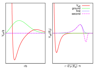
Figure 3: Division of the lowest effective adiabatic potential $V_{\mathrm{eff}}$ (solid line) for $E_{2}\rightarrow 0$ into $V_{\mathrm{sh}}$ (left) and $V_{\mathrm{lon}}$ (right). Range and strength of $V_{\mathrm{sh}}$ are defined through the range $b$ and strength $g$ of the two-body potential. Range and strength of $V_{\mathrm{lon}}$ are universal and defined through the two-body energy $E_{2}$. $V_{\mathrm{lon}}$ supports two universal three body states (dotted and dash-dotted lines). Here $V_{\mathrm{sh}}$ supports a third bound state (dashed) which becomes Borromean for $E_{2}=0$. If $V_{\mathrm{sh}}$ cannot support a bound state for $E_{2}=0$, a Borromean state does not occur.

3.3 Square well potentials

Eq. (30) qualitatively expresses the idea of the interplay between kinetic energy and interaction. A deep enough attraction inside a repulsive barrier, e.g. eq. (12), allows Borromean systems, since all three particles can benefit simultaneously from the attraction, without extending into the barrier. This is discussed for a schematic case in the Appendix. One would expect that potentials without an outside barrier, e.g. eq. (20), also must support Borromean binding for some $\lambda_{-},\lambda_{+}^{cr},R_{s}/R_{l}$. However extensive numerical searches did not reveal Borromean binding. Unfortunately, exploiting numerical search, we can not exclude it rigorously for all potentials without an outer barrier. However, using a rough estimate obtained from eq. (30) we can suggest a region where Borromean system might occur. To do so we establish a qualitative connection between a two-body square-well potential with infinite core and an effective three-body potential. We want to use only simple solvable potentials to suggest possibilities that unravel the general trend (see the appendix).

Using this connection we determine parameters of the two-body potentials that give three-body bound states with rms radius proportional to the range of the potential. To determine whether this is a Borromean state, we compare parameters of this potential with a two-body potential, that satisfies eq. (23). We present the result of this qualitative investigation on Fig. 4, where two-body bound states exist above the solid line, while dashed and dot-dashed lines represent parameters of the two-body potential that might allow three-body ground state with rms radius proportional to the range of the potential (see the Appendix). Thus Borromean systems are likely to exist below the two-body and above the three-body curves. The optimum configuration occurs when the two-body attraction is most effective for all pairs. By simple geometric considerations, this dictates that $R_{l}$ must be larger that $2R_{s}$. On the other hand $R_{s}/R_{l}$ can not go to zero, where as follows from Fig. 4 a two-body system is easily bound. This analysis suggests that the region where $R_{l}\sim 2R_{s}$ has to produce the largest Borromean window, because the negative part of the potential is deep enough to overcome the kinetic energy term, and radii do not deviate too much from each other, which allows the most effective attraction. This qualitative procedure unravels regions where three body Borromean state are most likely to exist.

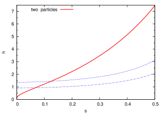
Figure 4: Axis and the solid red line is the same as on Fig. 2. Dashed and dot-dashed blue lines give an insight into the regions where three-body bound states with root mean square radius proportional to the range of the potential (see the Appendix) might exist. The space between solid and dashed (dot-dashed) line (when solid line is higher) gives a rough estimate for $h$ and $s$ that can support Borromean states.

3.4 Numerical illustrations

Our numerical procedure is based on the stochastic variational method with basis of correlated Gaussians. This procedure was proven to give accurate results suzuki1998 , however the convergence slows down for potentials with a hard core. Numerically convenient potentials are linear combinations of gaussians, because it allows calculation of matrix elements analytically. Moreover extensive numerical search with different potentials did not reveal Borromean states without an outer barrier. Thus, we choose a potential with outer barrier in the form $V_{\pm}=\frac{F\pm|F|}{2}$, with $F=\frac{\hbar^{2}}{2\mu b^{2}}\big{(}\exp(-0.5r^{2}/b^{2})-2\exp(-2r^{2}/b^{2})\big{)}$, where the net volume is zero. This potential is attractive for $r^{2}/b^{2}<\frac{2}{3}\ln 2$ and repulsive otherwise. We show in Fig. 5 the critical values for binding the two- and three-body systems as function of the attractive strength, $\lambda_{-}$. The straight line for the delta-shell potential is followed for small $\lambda_{-}$ for both two and three particles. The zero net volume behavior of $\lambda_{+}^{cr}\approx\lambda_{-}$ is found as expected in this region. All three curves begin to deviate around $\lambda_{-}\approx 0.7$, and the finite range potentials reveal their divergent character. We define the critical values, $\lambda_{-}^{cr}$ and $\Lambda_{-}^{cr}$, above which two and three-body bound states respectively are present independent of $\lambda_{+}$. This limit can be described by potentials of the form eq.(27) and we see numerically the expected ratio, $\Lambda_{-}^{cr}/\lambda_{-}^{cr}\sim 2/3$. When $\lambda_{-}>\lambda_{-}^{cr}$ the attractive pocket alone supports a two-body bound state.

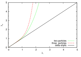
Figure 5: The two- and three-body critical strengths, $\lambda_{+}^{cr}$ (dashed line) and $\Lambda_{+}^{cr}$ (dot-dashed line), on the positive part of the potential as function of the strength on the negative part. The potential is $gV=\lambda_{+}V_{+}+\lambda_{-}V_{-}$ where $V_{\pm}$ are positive and negative parts of $\frac{\hbar^{2}}{2\mu b^{2}}\big{(}\exp(-0.5r^{2}/b^{2})-2\exp(-2r^{2}/b^{2})\big{)}$, respectively. Solid line represents results for delta-shell potential, i.e. $\lambda_{+}^{cr}=\lambda_{-}$.

At the threshold $\lambda_{+}=\lambda_{+}^{cr}$ two three-body states disappear into the continuum. They have the same threshold as the two-body system in complete analogy to weakly bound systems where the two and three-body thresholds are identical nielsen1999 ; bruch1979 . The difference for the deep potentials is that the Borromean state remains.

4 Experimental realization

From the discussion above it is obvious that Borromean systems in 2D are not as abundant as in 3D. In particular, we need an outer barrier and an attractive pocket. Systems where there is no outer barrier and those with non-positive net volume integral of the interaction are therefore out of the picture. This includes the case of neutral atoms in a plane which would have van der Waals-type attractive pockets and inner hard-core repulsion. A popular way to achieve long-range interactions is to use polar molecules lahaye2009 ; baranov2012 . In particular, layered systems with polar molcules have promising properties and have recently been stabilized experimentally miranda2011 . The geometric dipole-dipole interaction of polar molecules in a multilayer system supports a number of interesting few-body states jeremy2010 ; wang2006 ; klawunn2010 ; zinner2012-1 ; jeremy2012 ; artem2012 that are indicators of non-trivial many-body pairing potter2010 ; pikovski2010 ; zinner2012-2 . However, interlayer interactions always have zero net volume integral jeremy2010 , while the intralayer interactions are purely repulsive jeremy2012 and do not have the necessary pocket plus barrier structure.

In the following we list possible experimental setups where it could be possible to simultaneously maintain an outer barrier and a substantial inner attractive pocket.

The first option is to use cold ionized atoms in a two-dimensional geometry. Ideally this would be ions confined to live on a surface. Other interesting setups could be ions trapped near a surface szymanski2012 or in a Penning trap britton2012 . While these studies are mostly done with atoms in a crystal state, the few-body dynamics studied in the current paper requires that the ions also have motional degrees of freedom that are continuous in some range (or at least quasi-continuous if there is some weak confinement in the 2D plane of motion). To reach the Borromean regime, we have the outer barrier from the Coulomb repulsion of the ions. The inner attractive pocket would then need to be provided by short-range van der Waals interactions. This pocket is then required to sit at some small yet not too small distance in order to avoid the regime where everything is controlled by chemical reaction dynamics. What is particularly complicated about this proposal is the fact that the outer repulsive Coulomb barrier could be extremely large and render any inner attractive pocket irrelevant. This could possibly be counteracted through electron screening that lowers the Coulomb barrier. Here we imagine that a plasma of ions and electrons could be useful if it can be confined to 2D. A more realistic possiblity could be mobile impurities in solid-state system where the background electron density provides a screening effect.

A second, and presumably much easier, option is to use polar molecules in external fields. It has been predicted that applications of AC and DC fields in systems with particles that have non-zero permanent electric or magnetic dipole moments provides a way to taylor the inter-molecular interactions pfau2002 ; micheli2007 ; gorshkov2008 ; cooper2009 . In a squeezed geometry (quasi-2D), AC fields can be used to control the existance of two-body bound states for both bosonic and fermionic molecules, and correspondingly may result in bound three-body states of AC field dressed molecules huang2012 . What is needed here is the presence of both outer barrier and inner attractive pocket. As is discussed in Ref. micheli2007 this can be achieved by applying both an AC and a DC external field to the system. DC fields have been used to align polar molecules and control the overall magnitude of the dipole moment in two-dimensional systems miranda2011 and very recently the application of AC fields to the same geometry has been reported neyenhuis2012 . A combination of these two external influences could provide the potential profile necessary to produce and observe Borromean bound states in a 2D setup.

5 Conclusions

Two-body binding is easier achieved in 2D compared to 3D, because of the negative centrifugal barrier in the radial two-body Schrödinger equation. In all other spatial dimensions the centrifugal barrier is zero or positive. This feature makes 2D geometry a case of special interest.

We investigate possible few-body structures in 2D with the goal to find conditions for Borromean states. Thus, we search for the potentials that can support three, but not two-body bound states. Our focus is on potentials with positive and negative parts, as purely attractive potentials in 2D always support two-body bound state thus excluding Borromean states.

We show that the necessary condition for a potential to provide Borromean states is a substantial repulsive and attractive part. This is a consequence of the fact that near a two-body threshold a Borromean state is localised at small radii. This can happen only for potentials with substantial attraction to outweigh the kinetic energy of localisation. Moreover, our numerical search indicates that potentials without outer barrier are highly unlikely to support three-body states without a two-body state.

We conclude that experimental observation of Borromean systems in 2D is possible only for interactions that have an outer barrier, a substantial attractive region, and positive net volume. Polar molecules or ions in squeezed geometries are potential candidate systems for the occurence of low-dimensional Borromean states. A more speculative possibility is to look for Borromean signatures among impurities on a solid-state surface. The details of the experimental scenarios and which options are more viable goes beyond the current principle discussion and will be the focus of future studies.

Acknowledgements We thank F. F. Bellotti who was the first reader of the manuscript. This research was supported by grants from the Danish Council for Independent Research — Natural Sciences.

Appendix A Connections to the Hyperspherical Expansion

Here we qualitatively discuss the connection between an interparticle interaction and and the lowest adiabatic potential in the hyperspherical expansion method.

The hyperradial potential for three bosons interacting pairwise through a square well of radius $R_{0}$ and depth $V_{0}$ is determined semi-analytically for $s$-waves by solving trancendental algebraic equations jen96 . The hyperradius, $\rho$, is defined through two-body distances between pairs of the three particles which implies that the $3D$-procedure is directly applicable for $2D$ as well. The method divides the $\rho$-coordinate into four intervals, that is

(i) with $\rho<R_{0}/\sqrt{2}$, where all three two-particle distances are smaller than $R_{0}$.

(ii) $R_{0}/\sqrt{2}<\rho<R_{0}\sqrt{2/3}$, where at least 2 pairs interact, but configurations of 3 interacting pairs are also possible.

(iii) $R_{0}\sqrt{2/3}<\rho<R_{0}\sqrt{2}$, where at most 1 pair interacts, but configurations of 3 non-interacting pairs are also possible.

(iv) $R_{0}\sqrt{2}<\rho$, where at least 2 pairs don’t interact.

The hyperradial attractive potential in turn increases from $3V_{0}$ for $\rho=0$ through various continuous steps to a value less than $V_{0}$ at $\rho=R_{0}\sqrt{2}$. For larger $\rho$-values the potential approaches zero as $1/\rho^{2}$ until the scattering length is reached for $\rho\approx a\gg R_{0}$. For $\rho$ larger than $a$ the potential approaches zero even faster, that is in $3D$ as $\propto a/\rho^{3}$ and in $2D$ as $\propto a/(\rho^{3}\ln(\rho))$. These potentials must be supplemented by the centrifugal barrier term, which in $3D$ and $2D$ corresponds to effective angular momenta of $l^{*}=3/2$ and $l^{*}=1/2$, respectively.

The large-distance behavior in $3D$ allows a number of bound states provided the scattering length is sufficiently large. This means that it is possible to vary $R_{0}$ and $V_{0}$, where the scattering length is maintained to be much larger than $R_{0}$ while the volume is too small to support a bound two-body state. By increasing $a$ towards infinity, still for an unbound two-body system, the number of three-body bound states increase logarithmically towards infinity. This is the Efimov effect.

In $2D$ any, even infinitesimal, overall attractive potential provides a bound state. Thus, when the three-body potential can bind with the $l^{*}=1/2$-term, also the two-body system with $l^{*}=-1/2$-term is bound. No Borromean system can be constructed, and no Efimov effect exists, see subsection 3.2.

We consider now the more general two-body potential of an attractive square well of radius $R_{s}$ and depth $V_{s}$, and a repulsive barrier between $R_{s}$ and $R_{l}$ of height $V_{l}$. The most interesting combination in the present context is when $R_{l}>2R_{s}$, since then the large-distance configurations apply for the $s$-part of the potential before the short-distance behavior of the $l$-part has ceased to be present. In other words, the attraction contributes fully for all pairs when $\rho<R_{s}/\sqrt{2}$.

The volume, $h_{3}=k^{2}(R_{l}^{2}-R_{s}^{2})$, for the three-body potential is in general much larger than, $h_{2}$, for the two-body potential. We can roughly relate by $h_{3}\approx h_{2}f_{\mu}f_{V}f_{R}$, where $f_{\mu}=m/\mu=2$ is the ratio of the mass, $m$, in eq.(28), $f_{V}=\langle V\rangle/V_{0}\approx 2$ is the average three-body potential in units of $V_{0}$, and $f_{R}\approx(R_{0}\sqrt{2}/R_{0})^{2}=2$. Increase of the volume leads to the possibility of the Borromean binding.

In the limit of a huge barrier, $V_{l}$ is very large, we can then evaluate the condition for a bound three-body state. The hyperradial wave function, $J_{l=1}(\kappa\rho)$, for $l^{*}=3/2$ must have a node at $\rho=R_{s}/\sqrt{2}$, where $\kappa$ is the corresponding wave number. The dimensionless volume ratio is then, $h_{3}/h_{2}=f_{\mu}f_{V}f_{R}=2\times 3\times 1/2=3$. The node, $14.66$, is smaller than $3$ times the corresponding node, $5.78$ of the two-body wave function, $J_{l=0}(kr)$, which immedately implies that there is a window where three, but not two, particles are bound. Borromean systems exist when $4.89<h_{2}<5.78$, that is for small $s<0.5$.

Changing the sign of the two-body potential gives a repulsive core up to $R_{s}$ and afterwards until $R_{l}$ an attractive well. We use again the relation between two and three-body potentials where three-body binding must arise from the attractive part in the interval $R_{s}\sqrt{2}<\rho<R_{l}\sqrt{2}$. The limit of $s\rightarrow 0$ correspond to two-body potentials resembling an overall very weakly attractive potential. In this case Borromean systems cannot exist, see subsection 3.2.

Assuming an average potential strength of $2V_{l}$ we get, with $s_{3}=s_{2}=R_{s}/R_{l}$ that Borromean systems exist when $8h_{2}>h_{3}$. This comparison can be improved by replacing $2V_{l}$ by a weighted average of the attractive strength, $\langle V\rangle\approx\int Vrdr/\int rdr=19(1-36s^{2}/19)/[12(1-s^{2})]$. The average decreases with $s$ to a value of $10/9$ for $s=1/2$. This curve, shown in Fig.4 - dot-dashed line, allows a rather large window for Borromean states in an interval from $0.1<s<0.5$.

These estimates of restrictions are rather conservative. First they are only estimates, and second two other, so far neglected effects, oppose existence of Borromean states derived from the hyperspherical formalism. The first is that the approximation to use only the lowest adiabatic potential implies that the correct three-body energy must be lower. This is derived from the general theorem that the correct energy lie between the results from the lowest adiabatic potential with and without the diagonal non-adiabatic term. This tends to further narrow down the Borromean window.

The second effect is that the fraction of the 2D coordinate space where the distance between two particles is less than $R_{s}$ is $R_{s}^{2}/(2\rho^{2})$ for a given hyperradius. Then one of the attractions, $V_{l}$, should be replaced by the repulsion, $V_{s}$, in total amounting to $V_{l}\rightarrow V_{l}(1-s^{2}(1+V_{s}/V_{l})/3)$ when $\rho=R_{l}/\sqrt{2}$. For a larger $\rho=R_{l}\sqrt{2/3}$, the factor $1/3$ should be replaced by $3/8$. The requirement of an overall positive volume of the two-body potential provide the inequality $s^{2}(1+V_{s}/V_{l})>1$, which gives a limit on the reduction factor, that is at least $(1-s^{2}(1+V_{s}/V_{l})/3)<2/3$. Thus, we should further restrict the volumes by multiplying with $2/3$. This curve is also shown in Fig.4 (dashed line), leaving still room for Borromean states. However, a reduction by an additional factor of $2$ would close that window completely.

In conclusion, the features of the square well must be maintained in other potentials, that is with both attractive and repulsive parts. The conclusions are therefore much more general. Whether a small window is open for Borromean states in $2D$ without a confining outer barrier remains to be seen. The features of candidate potentials are that the ratio of attractive to repulsive volumes must be between $8$ and $15$. The ratio of repulsive to attractive strengths must be limited to be smaller than $1/s^{2}-1<V_{s}/V_{l}<2/s^{2}-1$.

References

- (1) M.V. Zhukov et al., Phys. Rep. 231, 151 (1993)
- (2) K. Riisager, Phys. Scr. T152, 014001 (2013)
- (3) J.-M. Richard, S. Fleck, Phys. Rev. Lett. 73, 1464 (1994)
- (4) S. Moszkowski, S. Fleck, A. Krikeb, L. Theußl, J.M. Richard, K. Varga, Phys. Rev. A 62, 032504 (2000)
- (5) L.D. Landau, E.M. Lifshitz: Quantum Mechanics, (Pergamon Press, Oxford, 1977)
- (6) J.A. Tjon, Phys. Rev. A 21, 1334 (1980)
- (7) S.K. Adhikari, A. Delfino, T. Frederico, I.D. Goldman, L. Tomio, Phys. Rev. A 37, 3666 (1988)
- (8) F. Cabral, L.W. Bruch, J. Chem. Phys. 70, 4669 (1979)
- (9) T.K. Lim, S. Nakaichi, Y. Akaishi, H. Tanaka H, Phys. Rev. A 22, 28 (1980)
- (10) E. Nielsen, D.V. Fedorov, A.S. Jensen, Few Body Systems 22, 15 (1999)
- (11) H.-W. Hammer, D.T. Son, Phys. Rev. Lett. 93, 250408 (2004)
- (12) D. Blume, Phys. Rev. B 72, 094510 (2005)
- (13) K. Helfrich, H.-W. Hammer, Phys. Rev. A 83, 052703 (2011)
- (14) O.I. Kartavtsev, A.V. Malykh, Phys. Rev. A 74, 042506 (2006)
- (15) F.F. Bellotti et al., J. Phys. B: At. Mol. Opt. Phys. 44, 205302 (2011)
- (16) F.F. Bellotti et al., Phys. Rev. A 85, 025601 (2012)
- (17) F.F. Bellotti et al., J. Phys. B: At. Mol. Opt. Phys. 46, 055301 (2013)
- (18) We consider potentials which are isotropic, fall off faster than at infinity, and are bounded. However, most of the results can be extended to potentials with infinite repulsion.
- (19) A.G. Volosniev, D.V. Fedorov, A.S. Jensen, N.T. Zinner, Phys. Rev. Lett. 106, 250401 (2011)
- (20) A.G. Volosniev, N.T. Zinner, D.V. Fedorov, A.S. Jensen, B. Wunsch, J. Phys. B: At. Mol. Opt. Phys. 44 250401 (2011)
- (21) W.G. Gibson, Phys. Lett. A 117, 107 (1986)
- (22) B. Simon, Ann. Phys. 97, 279 (1976)
- (23) J.R. Armstrong, N.T. Zinner, D.V. Fedorov, A.S. Jensen, Europhys. Lett. 91, 16001 (2010)
- (24) M. Abramowitz, I. Stegun: Handbook of Mathematical Functions with Formulas, Graphs, and Mathematical Tables (Dover, New York, 1964)
- (25) M.L. Cramer, L.W. Bruch, F. Cabral, J. Chem. Phys. 67, 1442 (1977)
- (26) D.V. Fedorov, A.S. Jensen, Phys. Rev. Lett. 71, 4103 (1993)
- (27) E. Nielsen, D.V. Fedorov, A.S. Jensen, Phys. Rev. A 56, 3287 (1997)
- (28) Y. Suzuki, K. Varga: Stochastic Variational Approach to Quantum-Mechanical Few-Body Problems (Springer, Berlin, 1998)
- (29) L.W. Bruch, J.A. Tjon, Phys. Rev. A 19, 425 (1979)
- (30) T Lahaye, C Menotti, L Santos, M Lewenstein, T Pfau, Rep. Prog. Phys. 72, 126401 (2009)
- (31) M.A. Baranov, M. Dalmonte, G. Pupillo, P. Zoller, Chemical Reviews 112, 5012 (2012)
- (32) M.G.H. de Miranda et al., Nature Phys. 7, 502 (2011)
- (33) D.-W. Wang, M.D. Lukin, E. Demler, Phys. Rev. Lett. 97, 180413 (2006)
- (34) M. Klawunn, A. Pikovski, L. Santos, Phys. Rev. A 82, 044701 (2010)
- (35) N.T. Zinner, J.R. Armstrong, A.G. Volosniev, D.V. Fedorov, A.S. Jensen, Few-Body Systems 53, 369 (2012)
- (36) J.R. Armstrong, N.T. Zinner, D.V. Fedorov, A.S. Jensen, Eur. Phys. J. D 66, 85 (2012)
- (37) A.G. Volosniev et al., arXiv:1112.2541 (Few-Body systems, in press, 2012)
- (38) A.C. Potter, E. Berg, D.-W. Wang, B.I. Halperin, E. Demler,Phys. Rev. Lett. 105, 220406 (2010)
- (39) A. Pikovski, M. Klawunn, G.V. Shlyapnikov, L. Santos, Phys. Rev. Lett. 105, 215302 (2010)
- (40) N.T. Zinner, B. Wunsch, D. Pekker, D.-W. Wang, Phys. Rev. A. 85, 013603 (2012)
- (41) B. Szymanski et al., Appl. Phys. Lett. 100, 171110 (2012)
- (42) J. W. Britton et al., Nature 484, 489 (2012).
- (43) S. Giovanazzi, A. Görlitz, and T. Pfau, Phys. Rev. Lett. 89, 130401 (2002).
- (44) A. Micheli, G. Pupillo, H.P. Büchler, and P. Zoller, Phys. Rev. A 76, 043604 (2007).
- (45) A.V. Gorshkov it et al., Phys. Rev. Lett. 101, 073201 (2008).
- (46) N.R. Cooper and G.V. Shlyapnikov, Phys. Rev. Lett. 103, 155302 (2009).
- (47) S.-J. Huang et al., Phys. Rev. A 85, 055601 (2012).
- (48) B. Neyenhuis et al., Phys. Rev. Lett. 109, 230403 (2012)
- (49) A.S. Jensen, E. Garrido, D.V. Fedorov, Few-Body Systems 22, 193 (1997)