Polarized Structure Functions and Two-Photon Physics at Super-B

Abstract:

The potential of polarized, high-luminosity, moderate-energy $e^{+}e^{-}$ colliders for performing unique measurements in fundamental QCD is described, with particular reference to the proposed Super-B facility. An extensive programme of 2-photon physics is proposed, focusing on measurements of the polarized photon structure functions $g_{1}^{\gamma}$ and $g_{2}^{\gamma}$ and pseudoscalar meson transition functions. The experimental requirements for Super-B to make the first measurement of the first moment sum rule for the off-shell polarized photon structure function $g_{1}^{\gamma}(x,Q^{2};K^{2})$ are described in detail. Cross-section formulae and experimental issues for investigations of NLO and higher-twist effects in $g_{1}^{\gamma}$ and $g_{2}^{\gamma}$ together with exclusive 2-photon meson production are presented. This programme of QCD studies complements the core mission of Super-B as a high-luminosity B factory investigating flavour physics and rare processes signaling new physics beyond the standard model.

1 Introduction

High-luminosity, moderate energy $e^{+}e^{-}$ colliders open a window on a wide and interesting range of phenomena in QCD. They provide an especially clean environment where many fundamental aspects of QCD itself can be studied without the complication of bound-state hadronic targets. With polarized beams, they provide the ideal conditions to study the polarized photon structure functions $g_{1}^{\gamma}$ and $g_{2}^{\gamma}$, including moment sum rules and higher-order perturbative QCD and higher-twist effects, $U(1)_{A}$ dynamics and anomalies, the gluon topological susceptibility, exclusive pseudoscalar meson production and transition functions, chiral symmetry breaking and vector meson dominance, amongst many others.

Super-B [2, 3, 4, 5] is a high-luminosity, asymmetric $e^{+}e^{-}$ collider to be built at the Cabibbo Laboratory at the University of Rome ‘Tor Vergata’ campus, with commissioning expected in 2017. It is conceived as a B factory, with asymmetric $e^{+}$ and $e^{-}$ beams with CM energy initially tuned to the $\Upsilon(4S)$ resonance at $\sqrt{s}=10.58~{}{\rm GeV}$ and luminosity $10^{36}~{}{\rm cm}^{-2}{\rm s}^{-1}$ corresponding to an annual integrated luminosity in excess of $12~{}{\rm ab}^{-1}$. It is designed to study precision flavour physics and rare events with a view to discovering signals of new physics beyond the standard model. The extensive scope of this physics programme is described in detail in ref.[3] while descriptions of the accelerator and detector can be found in refs.[4] and [5] respectively. Importantly, it is planned that from the outset the electrons in the low-energy ring will be polarized, with efficiencies of over 70% [6]. This will be achieved by injecting tranversely polarized electrons and using a system of spin rotators to produce a longitudinally polarized beam within the interaction region.

In this paper, we point out that in addition to its core flavour physics mission, Super-B has the potential to perform unique studies of polarization phenomena in QCD through a complementary programme of polarized 2-photon physics. To illustrate this potential, we describe in detail a number of QCD measurements, focusing on the polarized photon structure functions $g_{1}^{\gamma}$ and $g_{2}^{\gamma}$ and pseudoscalar meson transition functions, explaining the accelerator and detector requirements for these to be made at Super-B.

Foremost amongst these is the first moment sum rule for the polarized photon structure function $g_{1}^{\gamma}(x,Q^{2};K^{2})$, where $Q^{2}$ and $K^{2}$ are the invariant momenta of the scattered and target photon respectively, as measured in the inclusive process $e^{+}e^{-}\rightarrow e^{+}e^{-}X$ in the deep-inelastic regime (see Fig. 1). This was first proposed by Narison, Shore and Veneziano in 1992 [7, 8], though only now has collider technology evolved to the point where a detailed experimental verification has become possible. We emphasise that, in contrast to experiments using real back-scattered laser photons as the target, the target photons in $e^{+}e^{-}$ scattering are in principle virtual and indeed almost all the interesting QCD physics resides in the $K^{2}$-dependence of the sum rule. The sum rule can be written as [7, 9]:

$$\int_{0}^{1}dx~{}g_{1}^{\gamma}(x,Q^{2};K^{2})={1\over 18}{\alpha\over\pi}\left(1-{\alpha_{s}(Q^{2})\over\pi}\right)\\ \times\biggl{[}3F^{3}(K^{2})+F^{8}(K^{2})+8F^{0}(K^{2};\mu^{2})\exp\int_{t(K^{2})}^{t(Q^{2})}dt^{\prime}\gamma(\alpha_{s}(t^{\prime}))\biggr{]}\ ,$$ (1)

in terms of non-perturbative form factors $F^{a}(K^{2})$ which characterise the anomalous three-current AVV correlation function $\langle 0|J_{\mu 5}^{a}(0)~{}J_{\lambda}(k)~{}J_{\rho}(-k)|0\rangle$. Here, $\gamma(\alpha_{s})$ is the anomalous dimension of the flavour singlet axial current, $t(Q^{2})={1\over 2}\log(Q^{2}/\mu^{2})$, and we assume three dynamical quark flavours, so $a=3,8$ denote $SU(3)$ flavour generators with $a=0$ the singlet. The AVV correlator is an important quantity in non-perturbative QCD and encodes a wealth of information about anomalies, chiral symmetry breaking and the validity of widely used models such as vector meson dominance. First-principles theoretical calculations are challenging and the opportunity to compare with direct experimental measurements for a variety of external momenta will be valuable.

For real photons, $K^{2}=0$, electromagnetic gauge invariance implies the simple sum rule

$$\int_{0}^{1}dx~{}g_{1}^{\gamma}(x,Q^{2};0)=0\ ,$$ (2)

first derived by Bass [10] (see also refs.[7, 8, 11]). For target photons with invariant momenta in the range $m_{\rho}^{2}\ll K^{2}\ll Q^{2}$, the sum rule is determined entirely by the electromagnetic $U(1)_{A}$ anomaly with perturbative QCD corrections given by Wilson coefficients together with the anomalous dimension related to the QCD $U(1)_{A}$ anomaly. It was shown in ref.[7] that to NLO, i.e. $O(\alpha\alpha_{s})$,

$$\int_{0}^{1}dx~{}g_{1}^{\gamma}(x,Q^{2};K^{2})={2\over 3}{\alpha\over\pi}\biggl{[}1-{\alpha_{s}(Q^{2})\over\pi}+{4\over 9}\biggl{(}{\alpha_{s}(Q^{2})\over\pi}-{\alpha_{s}(K^{2})\over\pi}\biggr{)}\biggr{]}\ .$$ (3)

Note that the overall normalisation factor is $N_{c}\sum_{f}\hat{e}_{f}^{4}$, proportional to the fourth power of the quark charges $\hat{e}_{f}$, corresponding to the lowest order box diagram contributing to $g_{1}^{\gamma}$. This result was verified in refs.[12, 13] and subsequently extended to NNLO, $O(\alpha\alpha_{s}^{2})$, in ref.[14].

In order to verify the first moment sum rule experimentally, we require polarized beams and a sufficiently high luminosity to allow the spin asymmetry of the cross-section to be measured, recalling [7] that it is kinematically suppressed by a factor of $Q_{\rm min}^{2}/s$ relative to the total cross-section. This factor also explains why colliders with moderate CM energy $\sqrt{s}$ are favoured for this type of QCD spin physics. Identification of the target photon virtuality $K^{2}$ is most clearly done by tagging the target electron, though this is experimentally challenging for the small angles necessary to access the non-perturbative region $K^{2}\simeq m_{\rho}^{2}$. The perturbative sum rule (3), for $K^{2}\gtrsim 1~{}{\rm GeV}^{2}$ is more readily measurable. These experimental issues are discussed in detail in section 5, after we derive the relevant cross-section moment formulae in section 2. It is important here that all these formulae are derived without use of the conventional ‘equivalent photon’ formalism (see, e.g. refs. [15, 16], since the $K^{2}$-dependence of the target photon is crucial.

If the azimuthal angle between the planes of the scattered and target electrons is also measured, then we can identify the second polarized photon structure function $g_{2}^{\gamma}(x,Q^{2};K^{2})$. This is of additional theoretical interest since it receives contributions from both twist 2 and twist 3 operators in the OPE analysis of deep inelastic scattering. Following ref.[17], we show how to isolate the twist 3 contribution, then derive cross-section formulae to use the azimuthal angle dependence of the scattered electrons to distinguish the structure functions and determine $g_{2}^{\gamma}$.

In refs.[7, 8, 9, 18], it was shown how the non-perturbative form factors $F^{a}(K^{2})$ can be related to the off-shell transition functions $g_{P\gamma^{*}\gamma^{*}}(0,K^{2},K^{2})$ of the pseudoscalar mesons $P=\pi,\eta,\eta^{\prime}$. An important subtlety arises in the flavour singlet sector, where the QCD $U(1)_{A}$ anomaly means that the equivalent result for the $\eta^{\prime}$ also involves the gluon topological susceptibility, the key non-perturbative quantity which controls much of the $U(1)_{A}$ dynamics of QCD. In fact, the pseudoscalar meson transition functions can be measured directly for different photon virtualities via the exclusive two-photon production reaction $e^{+}e^{-}\rightarrow e^{+}e^{-}P$ (see Fig. 2) even with unpolarized beams. Such measurements have already been made at CELLO [19], CLEO [20] and BABAR [21, 22, 23] for transition functions $g_{P\gamma^{*}\gamma}(m_{P}^{2},Q^{2},0)$ with one virtual and one assumed real photon. Here, in section 4, we derive cross-section formulae relevant to polarized beams and discuss what may be learned more generally from measurements of meson transition functions at Super-B. In addition to their intrinsic interest, these are important in theoretically determining the virtual light-by-light $\gamma^{*}\gamma^{*}\rightarrow\gamma^{*}\gamma^{*}$ scattering amplitude, which is itself a key part of the hadronic contribution which is the major uncertainty in reconciling theoretical predictions with experimental measurements of $g-2$ for the muon [24].

This theoretical analysis of the polarized photon structure functions and pseudoscalar meson transition functions is presented in sections 2-4, with extensive reference to our earlier papers [7, 8, 9, 18, 25, 26, 27]. See also refs. [28, 29, 30, 31, 32, 33, 34, 17, 13, 14, 35] for a selection of further papers on the $g_{1}^{\gamma}$ and $g_{2}^{\gamma}$ photon structure functions, mainly from a parton perspective. Here, our focus is on deriving cross-section formulae and investigating the experimental requirements to measure $g_{1}^{\gamma}(x,Q^{2};K^{2})$, $g_{2}(x,Q^{2};K^{2})$ and $g_{P\gamma*\gamma*}$ at a high-luminosity, polarized $e^{+}e^{-}$ collider. In the final section, we turn more specifically to Super-B and investigate the cross-sections and experimental cuts necessary to measure the first moment sum rule for $g_{1}^{\gamma}$ with  the design CM energy and luminosity. We will also consider what detector requirements are necessary to realise the full potential of Super-B as the collider of choice to investigate polarized QCD phenomenology.

2 Polarized Photon Structure Functions $g_{1}^{\gamma}$ and $g_{2}^{\gamma}$

In this section, we show how to determine the polarized photon structure functions $g_{1}^{\gamma}(x,Q^{2};K^{2})$ and $g_{2}^{\gamma}(x,Q^{2};K^{2})$ and their moments from the inclusive process $e^{+}e^{-}\rightarrow e^{+}e^{-}X~{}{\rm(hadrons)}$ shown in Fig. 1.

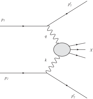
Figure 1: Kinematics for the inclusive two-photon reaction $e^{+}e^{-}\rightarrow e^{+}e^{-}X~{}{\rm hadrons}$.

We begin with some kinematics. The total cross-section is given by integrating over the phase space of the scattered electrons, a total of 6 degrees of freedom. However, by symmetry only the relative azimuthal angle $\phi=\phi_{1}-\phi_{2}$ of the scattering planes of the electrons is physically relevant, so we need to specify only 5 Lorentz invariants. We choose these to be $Q^{2}=-q^{2}$, $K^{2}=-k^{2}$, $\nu_{e}=p_{2}.q$, $\bar{\nu}_{e}=p_{1}.k$ and $\nu=k.q$. The deep-inelastic limit is $Q^{2},\nu_{e},\nu\rightarrow\infty$ with $x_{e}=Q^{2}/2\nu_{e}$ and $x=Q^{2}/2\nu$ fixed. Note that while we use the analogous notation for the ‘target’ electron, neither $K^{2}$ nor $\bar{\nu}_{e}$ is assumed to be large, and indeed we are most interested in the regime $K^{2}/Q^{2}\ll 1$, with $K^{2}$ less than around 1 GeV².

In terms of the momenta and angles of the scattered electrons in the lab frame, we define $p_{1}^{\mu}=(E_{1},0,0,E_{1})$ and $p_{1}^{\prime\mu}=(E_{1}^{\prime},E_{1}^{\prime}\sin\theta_{1}\cos\phi_{1},E_{1}^{\prime}\sin\theta_{1}\sin\phi_{1},E_{1}^{\prime}\cos\theta_{1})$, in the limit where we neglect the electron mass, and similarly for $p_{2}^{\mu}$ and $p_{2}^{\prime\mu}$, noting that for an asymmetric collider like Super B, $E_{1}\neq E_{2}$. We then have, with $s=(p_{1}+p_{2})^{2}=4E_{1}E_{2}$,

$$Q^{2} =4E_{1}E_{1}^{\prime}\sin^{2}{\theta_{1}\over 2}~{}~{}~{}~{}~{}~{}~{}~{}~{}~{}~{}~{}~{}~{}~{}~{}~{}~{}~{}~{}~{}~{}~{}~{}~{}K^{2}=4E_{2}E_{2}^{\prime}\sin^{2}{\theta_{2}\over 2}$$

$$\nu_{e} =2E_{2}\left(E_{1}-E_{1}^{\prime}\cos^{2}{\theta_{1}\over 2}\right)~{}~{}~{}~{}~{}~{}~{}~{}~{}~{}~{}~{}~{}~{}\bar{\nu}_{e}=2E_{1}\left(E_{2}-E_{2}^{\prime}\cos^{2}{\theta_{2}\over 2}\right)$$

$$\nu =\frac{2}{s}\bigl{(}\nu_{e}\bar{\nu}_{e}+{1\over 4}K^{2}Q^{2}\bigr{)}+k_{T}q_{T}\cos\phi$$ (4)

where we define $q_{T}(k_{T})$ as the magnitude of the transverse component of $q^{\mu}(k^{\mu})$, so that

$$q_{T}^{2}=Q^{2}\Bigl{(}1-{2\nu_{e}\over s}\Bigr{)}\ ,~{}~{}~{}~{}~{}~{}~{}~{}~{}~{}~{}~{}~{}~{}~{}~{}~{}~{}k_{T}^{2}=K^{2}\Bigl{(}1-{2\bar{\nu}_{e}\over s}\Bigr{)}\ .$$ (5)

The on-shell condition for the electrons determines $p_{1}.q=-{1\over 2}Q^{2}$ and $p_{2}.k=-{1\over 2}K^{2}$ so these are not independent variables. Also note that $\nu=\tfrac{1}{2}(Q^{2}+K^{2}+W^{2})$, where $W^{2}$ is the total hadronic invariant momentum.

The complete set of 5 kinematic variables is therefore the measurable quantities $E_{1}^{\prime},\theta_{1},E_{2}^{\prime},\theta_{2},\phi$, which determine the invariants $Q^{2},K^{2},\nu_{e},\bar{\nu}_{e},\nu$. We will be concerned with cross-sections that are differential with respect to different subsets of these 5 invariants. Note that the azimuthal dependence $\phi$ is encoded in $\bar{\nu}_{e}$ once $\nu_{e}$ and $\nu$ are fixed. For the theoretical discussion, we assume that the target electron is tagged, with $E_{2}^{\prime}$ and $\theta_{2}$ (as well as $\phi$) being measured directly. The experimental issue of whether this is possible for the interesting range of $K^{2}$, or whether it would be necessary to try to reconstruct the scattered target electron momentum from a knowledge of the total hadronic momentum, is discussed later.

The photon structure functions are defined from the Green function $T_{\mu\nu\lambda\rho}(q,k)=\langle 0|J_{\mu}(q)J_{\nu}(-q)A_{\lambda}(k)A_{\rho}(-k)|0\rangle$. There are two independent Lorentz structures, which we denote [12, 13] as $I_{\mu\nu\lambda\rho}$ and $J_{\mu\nu\lambda\rho}$ where

$$I_{\mu\nu\lambda\rho} =-\nu\epsilon_{\mu\nu\alpha\gamma}\epsilon_{\lambda\rho\beta}{}^{\gamma}q^{\alpha}k^{\beta}$$

$$J_{\mu\nu\lambda\rho} =I_{\mu\nu\lambda\rho}-\epsilon_{\mu\nu\alpha\gamma}\epsilon_{\lambda\rho\beta\delta}q^{\alpha}q^{\beta}k^{\gamma}k^{\delta}\ .$$ (6)

The structure functions $g_{1}^{\gamma}$ and $g_{2}^{\gamma}$ are then given in terms of the antisymmetric part of $T_{\mu\nu\lambda\rho}$ as follows:

$$\tfrac{1}{\pi}\operatorname{Im}T_{\mu\nu\lambda\rho}^{A}={1\over{2K^{4}\nu^{2}}}\Bigl{[}g_{1}^{\gamma}(x,Q^{2};K^{2})~{}I_{\mu\nu\lambda\rho}~{}+~{}g_{2}^{\gamma}(x,Q^{2};K^{2})~{}J_{\mu\nu\lambda\rho}\Bigr{]}\ .$$ (7)

The usual leptonic tensor for electrons with helicity $h_{1}/2$, where $h_{1}=\pm 1$, is defined as:

$$L_{\lambda\rho}(p_{1},h_{1};q)=4p_{1\lambda}p_{1\rho}-2(p_{1\lambda}q_{\rho}-p_{1\rho}q_{\lambda})+q^{2}g_{\lambda\rho}+2ih_{1}\epsilon_{\lambda\rho\sigma\tau}p_{1}^{\sigma}q^{\tau}\ ,$$ (8)

and it is convenient to define the antisymmetric part,

$$L^{A}_{\lambda\rho}(p_{1};q)=2i\epsilon_{\lambda\rho\sigma\tau}p_{1}^{\sigma}q^{\tau}\ .$$ (9)

We then find

$$\tfrac{1}{\pi}\operatorname{Im}T_{\mu\nu\lambda\rho}^{A}(q,k)L^{\lambda\rho}(p_{2},h_{2};k)=-2ih_{2}K^{2}{1\over\nu}\epsilon_{\mu\nu\alpha\gamma}q^{\gamma}\left[g_{1}^{\gamma}(p_{2}^{\alpha}-\tfrac{1}{2}k^{\alpha})+g_{2}^{\gamma}\left(p_{2}^{\alpha}-{\nu_{e}\over\nu}k^{\alpha}\right)\right]$$ (10)

and (compare ref.[17], appendix A)

$$L^{\mu\nu}(p_{1},h_{1};q)\tfrac{1}{\pi}\operatorname{Im}T_{\mu\nu\lambda\rho}^{A}(q,k)L^{\lambda\rho}(p_{2},h_{2};k)\\ =-4h_{1}h_{2}K^{2}Q^{2}\frac{1}{\nu^{2}}\left[g_{1}^{\gamma}(s+\tfrac{1}{2}\nu-\nu_{e}-\bar{\nu}_{e})+g_{2}^{\gamma}\left(s-\frac{2\nu_{e}\bar{\nu}_{e}}{\nu}\right)\right]\ .$$ (11)

The cross-section polarization asymmetry $\Delta\sigma={1\over 2}\bigl{(}\sigma(++)-\sigma(+-)\bigr{)}$ is then given as an integral over $q$ and $k$ as follows:

$$\Delta\sigma=\frac{\alpha^{3}}{4\pi^{2}}\frac{1}{s}\int d^{4}q~{}\delta\left(p_{1}.q+\tfrac{1}{2}Q^{2}\right)~{}\int d^{4}k~{}\delta\left(p_{2}.k+\tfrac{1}{2}K^{2}\right)\\ \times~{}\frac{1}{Q^{4}}L_{A}^{\mu\nu}(p_{1};q)\tfrac{1}{\pi}\operatorname{Im}T_{\mu\nu\lambda\rho}^{A}(q,k)L_{A}^{\lambda\rho}(p_{2};k)\ .$$ (12)

Changing variables in the $\int d^{4}q$ integration, including the Jacobian factor $1/s$, and integrating over the irrelevant azimuthal angle $\int d\phi_{1}=2\pi$ using the cylindrical symmetry, we find

$$\Delta\sigma={\alpha^{3}\over 2\pi}~{}\frac{1}{s^{2}}\int dQ^{2}\int d\nu_{e}\int d^{4}k~{}\delta\left(p_{2}.k+\tfrac{1}{2}K^{2}\right)\\ \times\frac{1}{Q^{4}}L_{A}^{\mu\nu}(p_{1};q)\tfrac{1}{\pi}\operatorname{Im}T_{\mu\nu\lambda\rho}^{A}(q,k)L_{A}^{\lambda\rho}(p_{2};k)\ .$$ (13)

(i)  $g_{1}^{\gamma}(x,Q^{2};K^{2})$ and cross-section moments:

The first structure function $g_{1}^{\gamma}(x,Q^{2};K^{2})$ and its moments can be isolated by measuring the differential cross-section $d^{3}\Delta\sigma/dQ^{2}dx_{e}dK^{2}$. To see this, note that under the full $\int d^{4}k$ integral we can effectively substitute $\bar{\nu}_{e}\rightarrow s\nu/2\nu_{e}+O(K^{2}/Q^{2})$. The $g_{2}^{\gamma}$ dependence then drops out of eq.(11), while the coefficient of $g_{1}^{\gamma}$ reorganises into the familiar Altarelli-Parisi splitting function $\Delta P_{\gamma e}(z)=2-z$, where $z=x_{e}/x$, and the standard kinematical factor $\left(1-Q^{2}/2x_{e}s\right)$ which arises in polarized cross-sections. Then, rewriting the $\int d^{4}k$ in terms of the invariants $K^{2},\nu$ and the azimuthal angle $\phi_{2}$, which we can then integrate over, we finally find:

$$\Delta\sigma={\alpha^{3}\over s}\int_{0}^{\infty}{dQ^{2}\over Q^{2}}\int_{0}^{1}{dx_{e}\over x_{e}}\int_{0}^{\infty}{dK^{2}\over K^{2}}\int_{x_{e}}^{1}{dx\over x}~{}\Delta P_{\gamma e}\left({x_{e}\over x}\right)~{}g_{1}^{\gamma}(x,Q^{2};K^{2})~{}\left(1-{Q^{2}\over 2x_{e}s}\right)\ ,$$ (14)

reproducing the result quoted in refs.[7, 9]. In particular, $x$-moments of the structure function $g_{1}^{\gamma}(x,Q^{2};K^{2})$ can be measured in terms of the $x_{e}$-moments of the polarization asymmetry of the differential cross-section as follows:

$$\int_{0}^{1}dx_{e}~{}x_{e}^{n}~{}{d^{3}\Delta\sigma\over dQ^{2}dx_{e}dK^{2}}={\alpha^{3}\over sQ^{2}K^{2}}\int_{0}^{1}dz~{}z^{n-1}\Delta P_{\gamma e}(z)~{}\int_{0}^{1}dx~{}x^{n-1}~{}g_{1}^{\gamma}(x,Q^{2};K^{2})\ ,$$ (15)

where the integral over the splitting function factorises. (For simplicity, we have assumed here that $Q^{2}/2x_{e}s\ll 1$ though this factor could easily be retained.) In particular, for the first moment we have simply

$$\int_{0}^{1}dx_{e}~{}{d^{3}\Delta\sigma\over dQ^{2}dx_{e}dK^{2}}={3\over 2}{\alpha^{3}\over sQ^{2}K^{2}}\int_{0}^{1}dx~{}g_{1}^{\gamma}(x,Q^{2};K^{2})\ ,$$ (16)

the key point being that the cross-section is differential w.r.t. the standard DIS variables $Q^{2},x_{e}$ and the target photon virtuality $K^{2}$ only, but with the dependence on the azimuthal angle $\phi$ integrated out.

(ii)  Azimuthal dependence and $g_{2}^{\gamma}(x,Q^{2};K^{2})$:

Alternatively, we may retain the explicit dependence on the azimuthal scattering angle in the differential cross-sections, which allows us to measure the second polarized structure function $g_{2}^{\gamma}(x,Q^{2};K^{2})$. This time, we re-express the $\int d^{4}k$ in eq.(13) directly as an integral over the invariants $K^{2},\nu$ and $\bar{\nu}_{e}$, which encodes the $\phi$-dependence. Rearranging terms, we find:

$$\Delta\sigma=\frac{\alpha^{3}}{\pi}\frac{1}{s}\int_{0}^{\infty}\frac{dQ^{2}}{Q^{2}}\int_{0}^{1}\frac{dx_{e}}{x_{e}}\int_{0}^{\infty}\frac{dK^{2}}{K^{2}}\int_{0}^{1}\frac{d\bar{x}_{e}}{\bar{x}_{e}}\int_{x_{e}}^{1}\frac{dx}{x}~{}{\hat{J}}\\ \times\left[g_{1}^{\gamma}\Big{(}2-\frac{x_{e}}{x}\Big{)}\left(1-\frac{Q^{2}}{2x_{e}s}\right)+\Big{(}2g_{2}^{\gamma}+\frac{x_{e}}{x}g_{1}^{\gamma}\Big{)}\left(1-\frac{xK^{2}}{x_{e}\bar{x}_{e}s}\right)\right]\ ,$$ (17)

where $\hat{J}=\nu_{e}\bar{\nu}_{e}J$, with the Jacobian factor $J$ (which we shall use explicitly in the section on pseudoscalar meson production) given by

$$J^{-1}=2|\epsilon_{\alpha\beta\gamma\delta}p_{1}^{\alpha}p_{2}^{\beta}q^{\gamma}k^{\delta}|=sk_{T}q_{T}\sin\phi\ ,$$ (18)

or alternatively,

$$J^{-2}=K^{2}Q^{2}(s-2\nu_{e})(s-2\bar{\nu}_{e})-4\left(\tfrac{1}{2}s\nu-\nu_{e}\bar{\nu}_{e}-\tfrac{1}{4}K^{2}Q^{2}\right)^{2}\ .$$ (19)

Note that the first term in eq.(17) is the same as before, while the factor

$$\left(1-\frac{xK^{2}}{x_{e}\bar{x}_{e}s}\right)=\left(1-\frac{2\nu_{e}\bar{\nu}_{e}}{s\nu}\right)=\frac{1}{s\nu}\left(sk_{T}q_{T}\cos\phi+\tfrac{1}{2}K^{2}Q^{2}\right)$$ (20)

encodes the azimuthal dependence and allows $g_{2}^{\gamma}$ to be determined from the differential cross-section asymmetry.

(iii)  Operator product expansion and sum rules:

In the deep-inelastic limit, the Green function $T_{\mu\nu\lambda\rho}(q,k)$ can be evaluated using the usual OPE for two electromagnetic currents,

$$iJ_{\mu}(q)J_{\nu}(-q)=-i\epsilon_{\mu\nu\alpha\sigma}q^{\alpha}\sum_{n=1,~{}{\rm odd}}\left(\frac{2}{Q^{2}}\right)^{n}q_{\mu_{2}}\ldots q_{\mu_{n}}\\ \times\left[\sum E_{2,n}(Q^{2})R_{2,n}^{\sigma\mu_{2}\ldots\mu_{n}}(0)+\sum E_{3,n}(Q^{2})R_{3,n}^{\sigma\mu_{2}\ldots\mu_{n}}(0)\right]\ ,$$ (21)

where $R_{2,n}$ and $R_{3,n}$ are respectively twist 2 and twist 3 and we have shown only the odd-parity operators, which contribute to $g_{1}^{\gamma}$ and $g_{2}^{\gamma}$. Form factors $\hat{R}_{2,n}(K^{2})$ and $\hat{R}_{3,n}(K^{2})$ are then defined as:

$$\langle 0|R_{2,n}^{\sigma\mu_{2}\ldots\mu_{n}}(0)A_{\lambda}(k)A_{\rho}(-k)|0\rangle =\frac{i}{K^{4}}{\cal S}\left[\hat{R}_{2,n}(K^{2})k^{\mu_{2}}\ldots k^{\mu_{n}}\epsilon^{\delta}{}_{\beta\lambda\rho}k^{\beta}\right]-{\rm traces}$$ (22)

$$\langle 0|R_{3,n}^{\sigma\mu_{2}\ldots\mu_{n}}(0)A_{\lambda}(k)A_{\rho}(-k)|0\rangle =\frac{i}{K^{4}}{\cal A}\left[\hat{R}_{2,n}(K^{2})k^{\mu_{2}}\ldots k^{\mu_{n}}\epsilon^{\delta}{}_{\beta\lambda\rho}k^{\beta}\right]-{\rm traces}\ .$$ (23)

With these definitions, we find [17]

$$T_{\mu\nu\lambda\rho}(q,k)=\sum_{n=1,{\rm odd}}\frac{1}{K^{4}}\left(\frac{2}{Q^{2}}\right)^{n}\nu^{n-2}\bigg{[}\sum E_{2,n}(Q^{2})\hat{R}_{2,n}(K^{2})\left(I_{\mu\nu\lambda\rho}-\frac{n-1}{n}J_{\mu\nu\lambda\rho}\right)\\ +\sum E_{3,n}(Q^{2})\hat{R}_{3,n}(K^{2})\frac{n-1}{n}J_{\mu\nu\lambda\rho}\bigg{]}\ ,$$ (24)

and therefore identify the structure functions as:

$$g_{1}^{\gamma}(x,Q^{2};K^{2}) =\frac{2}{\pi}\operatorname{Im}\sum_{n=1,~{}{\rm odd}}\sum E_{2,n}(Q^{2})\hat{R}_{2,n}(K^{2})x^{-n}$$ (25)

$$g_{2}^{\gamma}(x,Q^{2};K^{2}) =\frac{2}{\pi}\operatorname{Im}\sum_{n=1,~{}{\rm odd}}\frac{n-1}{n}\left[\sum E_{3,n}(Q^{2})\hat{R}_{3,n}(K^{2})-\sum E_{2,n}(Q^{2})\hat{R}_{2,n}(K^{2})\right]x^{-n}$$ (26)

The moment sum rules follow immediately. For the first structure function, we have

$$\int_{0}^{1}dx~{}x^{n-1}g_{1}^{\gamma}(x,Q^{2};K^{2})=\sum E_{2,n}(Q^{2})\hat{R}_{2,n}(K^{2})\ .$$ (27)

The important first moment sum rule is then

$$\int_{0}^{1}dx~{}g_{1}^{\gamma}(x,Q^{2};K^{2})=\sum_{r=3,8,0}E^{r}_{2,1}(Q^{2})\hat{R}^{r}_{2,1}(K^{2})\ ,$$ (28)

where the only operators contributing for $n=1$ are the axial currents $J_{\mu 5}^{r}$, with form factors defined from the three-current AVV Green function:

$$4\pi\alpha\langle 0|J_{\mu 5}^{r}(0)J_{\lambda}(k)J_{\rho}(-k)|0\rangle=i\epsilon_{\lambda\rho\mu\alpha}k^{\alpha}\hat{R}_{2,1}^{r}(K^{2})\ .$$ (29)

For the second structure function, we have the moment sum rule [17]

$$\int_{0}^{1}dx~{}x^{n-1}g_{2}^{\gamma}(x,Q^{2};K^{2})=\frac{n-1}{n}\left[\sum E_{3,n}(Q^{2})\hat{R}_{3,n}(K^{2})-\sum E_{2,n}(Q^{2})\hat{R}_{2,n}(K^{2})\right]\ .$$ (30)

It follows immediately that the first moment of $g_{2}^{\gamma}$ vanishes,

$$\int_{0}^{1}dx~{}g_{2}^{\gamma}(x,Q^{2};K^{2})=0\ .$$ (31)

This is the Burkhardt-Cottingham sum rule [37]. Following ref.[17], we can also isolate the contribution of the twist 3 operators. If we define the function $\bar{g}_{2}^{\gamma}$ as the function whose moments are given by the twist 3 terms on the r.h.s. of eq.(30), it is straightforward to show that

$$\bar{g}_{2}^{\gamma}=g_{2}^{\gamma}+g_{1}^{\gamma}-\int_{x}^{1}\frac{dx^{\prime}}{x^{\prime}}~{}g_{1}^{\gamma}(x^{\prime},Q^{2};K^{2})\ .$$ (32)

The second two terms, which therefore represent (minus) the twist 2 contribution to $g_{2}^{\gamma}$, reproduce the Wandzura-Wilczek [38] relation.

For our purposes, we have therefore shown how a measurement of the azimuthal dependence of the differential cross-section asymmetry at a polarized $e^{+}e^{-}$ collider such as Super B enables the photon structure function $g_{2}^{\gamma}$ to be measured as well as $g_{1}^{\gamma}$. The relation (32) then provides a theoretically clean decomposition allowing the contribution of the twist 3 operators in the OPE to be isolated and studied in detail.

3 First Moment Sum Rule for $g_{1}^{\gamma}(x,Q^{2};K^{2})$

The most interesting direct QCD measurement that could be made at a high-luminosity polarized $e^{+}e^{-}$ collider is the first moment sum rule for $g_{1}(x,Q^{2};K^{2})$. As shown above, this probes the important anomalous 3-current AVV Green function, which encodes a wealth of information on $U(1)_{A}$ physics, gluon topology and the realisation of chiral symmetry (for a review, see ref. [18]).

There are two elements to the sum rule (28). First are the Wilson coefficients which are well-known in perturbative QCD and are given to $O(\alpha_{s})$ by

$$E_{2,1}^{r} =c^{(r)}\left(1-\frac{\alpha_{s}(Q^{2})}{\pi}\right)\ ,\hskip 56.9055ptr=3,8$$

$$E_{2,1}^{0} =c^{0)}\left(1-\frac{\alpha_{s}(Q^{2})}{\pi}\right)\exp\left[\int_{0}^{t}dt^{\prime}\gamma\left(\alpha_{s}(t^{\prime})\right)\right]\ ,$$ (33)

where $t=\frac{1}{2}\log\frac{Q^{2}}{\mu^{2}}$. For $N_{c}=3$ and with $N_{f}=3$ effective dynamical flavours, where $r=3,8$ labels the $SU(3)_{f}$ generators and $r=0$ the singlet, the coefficients $c^{(r)}$ are determined by the quark charges: $c^{(3)}=\frac{1}{3}$,  $c^{(8)}=\frac{1}{3\sqrt{3}}$ and $c^{(0)}=\frac{2}{9}$. The flavour singlet current is not conserved because of the $U(1)_{A}$ anomaly, which gives rise to the non-vanishing anomalous dimension $\gamma=-\gamma_{0}\frac{\alpha_{s}}{4\pi}-\gamma_{1}\frac{\alpha_{s}^{2}}{(4\pi)^{2}}-\ldots$ with $\gamma_{0}=0$ and $\gamma_{1}=6N_{f}(N_{c}^{2}-1)/N_{c}=48$. It is important to note that this expansion only starts at $O(\alpha_{s}^{2})$. We also need the beta function: $\beta=-\beta_{0}\frac{\alpha_{s}^{2}}{4\pi}-\beta_{1}\frac{\alpha_{s}^{3}}{(4\pi)^{2}}-\ldots$ with $\beta_{0}=\frac{2}{3}(11N_{c}-2N_{f})=18$.

The second element is the AVV Green function itself. In general, this is given in terms of a set of six form factors $A_{1},\ldots,A_{6}$ by

$$-i\langle 0|J_{\mu 5}^{r}(p)J_{\lambda}(k_{1})J_{\rho}(k_{2})|0\rangle =A_{1}^{r}\epsilon_{\mu\lambda\rho\alpha}k_{1}^{\alpha}+A_{2}^{r}\epsilon_{\mu\lambda\rho\alpha}k_{2}^{\alpha}$$

$$+A_{3}^{r}\epsilon_{\mu\lambda\alpha\beta}k_{1}^{\alpha}k_{2}^{\beta}k_{2\rho}+A_{4}^{r}\epsilon_{\mu\rho\alpha\beta}k_{1}^{\alpha}k_{2}^{\beta}k_{1\lambda}$$

$$+A_{5}^{r}\epsilon_{\mu\lambda\alpha\beta}k_{1}^{\alpha}k_{2}^{\beta}k_{1\rho}+A_{6}^{r}\epsilon_{\mu\rho\alpha\beta}k_{1}^{\alpha}k_{2}^{\beta}k_{2\lambda}\ ,$$ (34)

where the form factors are functions of the invariant momenta: $A_{1}^{r}=A_{1}^{r}(p^{2},k_{1}^{2},k_{2}^{2})$, etc. For simplicity, we abbreviate $A_{i}^{r}(0,k^{2},k^{2})=A_{i}^{r}(K^{2})$ below. The form factor $\hat{R}_{2,1}^{r}(K^{2})$ in the first moment sum rule (28) is therefore simply

$$\hat{R}_{2,1}^{r}(K^{2})=4\pi\alpha\left(A_{1}^{r}(K^{2})-A_{2}^{r}(K^{2})\right)\ .$$ (35)

The $K^{2}=0$ limit of $\hat{R}_{2,1}^{r}$ is determined by electromagnetic current conservation [10, 7, 8, 11]. The Ward identity $\partial^{\lambda}J_{\lambda}=0$ applied to the AVV function implies

$$ik_{1}^{\lambda}\langle 0|J_{\mu 5}^{r}(p)J_{\lambda}(k_{1})J_{\rho}(k_{2})|0\rangle=0\ ,$$ (36)

and similarly for $k_{1}\rightarrow k_{2}$. Substituting the form factor decomposition, we find

$$A_{1}^{r} =A_{3}^{r}k_{2}^{2}+A_{5}^{r}\frac{1}{2}(p^{2}-k_{1}^{2}-k_{2}^{2})$$

$$A_{2}^{r} =A_{4}^{r}k_{1}^{2}+A_{6}^{r}\frac{1}{2}(p^{2}-k_{1}^{2}-k_{2}^{2})\ ,$$ (37)

so in the limit $p\rightarrow 0$, $k_{1}^{2}=k_{2}^{2}=-K^{2}$, the r.h.s. vanishes at $K^{2}\rightarrow 0$ provided none of the form factors is singular, as is the case in the absence of exactly massless Goldstone bosons coupling to $J_{\mu 5}^{r}$. It follows immediately that $\hat{R}_{2,1}^{r}(0)=0$, and so the first moment of $g_{1}^{\gamma}$ for real photons vanishes:

$$\int_{0}^{1}dx~{}g_{1}^{\gamma}(x,Q^{2};K^{2}=0)=0\ .$$ (38)

The asymptotic limit for large $K^{2}$ (while still retaining the DIS condition that $Q^{2}\gg K^{2}$) can be deduced using the renormalization group together with the anomalous chiral Ward identity for $J_{\mu 5}^{r}$. This is:

$$\partial^{\mu}J_{\mu 5}^{r}=d_{rst}m_{s}\phi_{5}^{t}+6Q\delta^{r0}+a^{(r)}\frac{\alpha}{8\pi}\tilde{F}^{\mu\nu}F_{\mu\nu}\ ,$$ (39)

where $\phi_{5}^{r}=\bar{\psi}T^{r}\gamma_{5}\psi$ and $Q=\frac{\alpha_{s}}{8\pi}{\rm tr}\tilde{G}^{\mu\nu}G_{\mu\nu}$ is the topological charge density. $G_{\mu\nu}$ and $F_{\mu\nu}$ are the gluon and electromagnetic field strengths, and the quark masses are written in $SU(3)_{f}$ notation as ${\rm diag}(m_{u},m_{d},m_{s})=\sum_{r=3,8,0}m_{r}T^{r}$ with $d_{rst}$ the usual $d$-symbols. The gluonic anomaly term involving $Q$ arises only for the $U(1)_{A}$ flavour singlet current $J_{\mu 5}^{0}$ while the final term is the usual electromagnetic axial anomaly, with coefficients $a^{(3)}=1$, $a^{(8)}=\frac{1}{\sqrt{3}}$ and $a^{(0)}=4$ determined by the quark charges. The AVV Green function therefore satisfies

$$ip^{\mu}\langle 0|J_{\mu 5}^{r}(p)J_{\lambda}(k_{1})J_{\rho}(k_{2})|0\rangle=d_{rst}m_{s}\langle 0|\phi_{5}^{r}(p)J_{\lambda}(k_{1})J_{\rho}(k_{2})|0\rangle\\ +6\delta^{r0}\langle 0|Q(p)J_{\lambda}(k_{1})J_{\rho}(k_{2})|0\rangle+a^{(r)}\frac{1}{8\pi^{2}}\epsilon_{\lambda\rho\alpha\beta}k_{1}^{\alpha}k_{2}^{\beta}\ ,$$ (40)

which in the limit $p\rightarrow 0$ implies

$$A_{1}^{r}(K^{2})-A_{2}^{r}(K^{2})=D^{r}(K^{2})+B^{r}(K^{2})+\frac{1}{8\pi^{2}}a^{(r)}\ ,$$ (41)

where $D^{r}$ and $B^{r}$ are form factors defined in the obvious way from the Green functions involving $\phi_{5}^{r}$ and $Q$. To determine the large $K^{2}$ behaviour, note that the form factors $A_{i}^{r}(K^{2})$ for the flavour non-singlet currents satisfy a homogeneous RG equation with the standard solution in terms of running couplings and masses, while for the flavour singlet there is an additional anomalous dimension contribution:

$$A_{i}^{r}(K^{2};\alpha_{s}(\mu);m) =A_{i}^{r}\big{(}\mu^{2};\alpha_{s}(t);e^{-t}m(t)\big{)}\hskip 85.35826ptr=3,8$$

$$A_{i}^{0}(K^{2};\alpha_{s}(\mu);m) =A_{i}^{0}\big{(}\mu^{2};\alpha_{s}(t);e^{-t}m(t)\big{)}\exp\left[-\int_{0}^{t}dt^{\prime}~{}\gamma(\alpha_{s}(t^{\prime}))\right]\ ,$$ (42)

where here $t=\frac{1}{2}\log\frac{K^{2}}{\mu^{2}}$. Similar results hold for $D^{r}(K^{2})$ and $B^{r}(K^{2})$. Clearly, therefore, in the limit $K^{2}\rightarrow\infty$ the mass term goes to zero and $D^{r}(K^{2})$ does not contribute. Moreover, for small $\alpha_{s}(t)$, the contribution $B^{r}(K^{2})$ of the topological charge term, which is $O(\alpha_{s}^{2})$, can be neglected at the NLO order we are working to here. (See [14] for a discussion of the sum rule at $O(\alpha_{s}^{2}\alpha)$.) We therefore deduce

$$\hat{R}_{2,1}^{r}(K^{2}\rightarrow\infty) =\frac{1}{2}a^{(r)}\frac{\alpha}{\pi}\hskip 85.35826ptr=3,8$$

$$\hat{R}_{2,1}^{0}(K^{2}\rightarrow\infty) =\frac{1}{2}a^{(0)}\frac{\alpha}{\pi}\exp\left[-\int_{0}^{t}dt^{\prime}~{}\gamma(\alpha_{s}(t^{\prime}))\right]\ .$$ (43)

The asymptotic form of the sum rule then follows by combining eq.(33) for the Wilson coefficients with eq.(43) for the form factors. We find [7]:

$$\int_{0}^{1}dx~{}g_{1}^{\gamma}(x,Q^{2};K^{2}\rightarrow\infty)=\sum_{r=3,8,0}E_{2,1}^{r}(Q^{2})\hat{R}_{2,1}^{r}(K^{2})\\ =\frac{1}{2}\frac{\alpha}{\pi}\left(1-\frac{\alpha_{s}(Q^{2})}{\pi}\right)\left[c^{(3)}a^{(3)}+c^{(8)}a^{(8)}+c^{(0)}a^{(0)}\exp\bigg{[}\int_{t(K)}^{t(Q)}dt^{\prime}~{}\gamma(\alpha_{s}(t^{\prime}))\bigg{]}\right]\ .$$ (44)

Finally, using $\frac{\alpha_{s}(t)}{4\pi}\simeq\frac{1}{\beta_{0}t}$ and substituting for the $c^{(r)}$ and $a^{(r)}$ coefficients, we obtain the result for $N_{c}=N_{f}=3$ QCD at $O(\alpha_{s}\alpha)$ quoted in the introduction [7]:

$$\int_{0}^{1}dx~{}g_{1}^{\gamma}(x,Q^{2};K^{2}\rightarrow\infty)=\frac{2}{3}\frac{\alpha}{\pi}\left(1-\frac{\alpha_{s}(Q^{2})}{\pi}\right)\left[1+\frac{4}{9}\left(\frac{\alpha_{s}(Q^{2})}{\pi}-\frac{\alpha_{s}(K^{2})}{\pi}\right)\right]\ .$$ (45)

Note that the overall coefficient is $N_{c}\sum_{f}\hat{e}_{f}^{2}$, i.e. proportional to the fourth power of the quark charges $\hat{e}_{f}$ as given by the lowest-order box diagram contributing to $g_{1}^{\gamma}$.

For intermediate values of $K^{2}$, we may rewrite the sum rule in the convenient form

$$\int_{0}^{1}dx~{}g_{1}^{\gamma}(x,Q^{2};K^{2})=\frac{1}{18}\frac{\alpha}{\pi}\left(1-\frac{\alpha_{s}(Q^{2})}{\pi}\right)\\ \times\left[3F^{3}(K^{2})+F^{8}(K^{2})+8F^{0}(K^{2};\mu^{2}=K^{2})\exp\bigg{[}\int_{t(K)}^{t(Q)}dt^{\prime}~{}\gamma(\alpha_{s}(t^{\prime}))\bigg{]}\right]\ ,$$ (46)

where we have introduced normalised form factors $F^{r}(K^{2})$ defined by

$$A_{1}^{r}(K^{2})-A_{2}^{r}(K^{2})=\frac{1}{8\pi^{2}}a^{(r)}F^{r}(K^{2})\ .$$ (47)

Note that in anomalous flavour singlet sector, with the choice of anomalous dimension factor in eq.(47), the renormalization scale in $F^{0}(K^{2};\mu^{2})$ is specified as $\mu^{2}=K^{2}$.

The form factors $F^{r}(K^{2})$ therefore interpolate between 0 for $K^{2}=0$ and 1 for asymptotically large $K^{2}$. The full momentum dependence of the sum rule for $g_{1}(x,Q^{2};K^{2})$ is governed by these form factors, which are in turn determined by the AVV Green finction. A non-perturbative, first-principles calculation of this 3-current Green function would therefore give a complete prediction for the first moment sum rule for arbitrary photon virtuality $K^{2}$.

In practice, this is still beyond current techniques and represents a challenge to lattice gauge theory, QCD spectral sum rules, AdS/QCD and other non-perturbative approaches to QCD. Indeed, this emphasises the importance of a direct experimental measurementof the sum rule and the form factors $F^{r}(K^{2})$. As an interim measure we can adopt a phenomenological approach, modelling the form factor by a simple interpolating formula such as $F^{r}(K^{2})\simeq K^{2}/(K^{2}+M^{2})$ for some characteristic crossover scale $M^{2}$. For heavy quarks, this would be the quark mass itself. However, for the light quarks, due to chiral symmetry breaking, we expect $M^{2}$ to be a typical hadronic scale, viz. $M^{2}\sim m_{\rho}^{2}$ for $F^{3}(K^{2})$. This can be supported by a simple OPE argument [7, 9]. If we evaluate the 3-current Green function by inserting an intermediate pseudoscalar meson, then write the OPE for the remaining electromagnetic currents for large $K^{2}$, we have

$$\langle\pi|J_{\lambda}(k)J_{\rho}(-k)|0\rangle=-\frac{2}{K^{2}}\epsilon_{\lambda\rho\alpha}{}^{\mu}k^{\alpha}E_{2,1}^{3}(K^{2})\langle\pi|J_{\mu 5}^{3}(0)|0\rangle+\ldots\ ,$$ (48)

which implies

$$F^{3}(K^{2}\rightarrow\infty)=1-\frac{(4\pi)^{2}}{3}f_{\pi}^{2}\frac{1}{K^{2}}+\ldots$$ (49)

The crossover scale is then identified from this expansion as $M^{2}\simeq\frac{(4\pi)^{2}}{3}f_{\pi}^{2}\sim m_{\rho}^{2}$, as would be expected in general terms from vector meson dominance.

4 Two-photon physics and pseudoscalar mesons

In this section, we consider other aspects of polarized two-photon physics accessible at Super B, with a special focus on the pseudoscalar mesons $P=\pi,\eta,\eta^{\prime}$ and their radiative transition functions $g_{P\gamma\gamma}(k_{1}^{2},k_{2}^{2})$. As we shall see, these may be measured for complementary values of the photon invariant momenta $k_{1}^{2}$ and $k_{2}^{2}$ either from the form factors arising in the $g_{1}^{\gamma}$ moment sum rule or by direct two-photon production of the pseudoscalar mesons.

(i)  Pseudoscalar mesons and the $g_{1}^{\gamma}(x,Q^{2};K^{2})$ sum rule:

In the first approach, we use familiar PCAC ideas to rewrite the form factors characterising the 3-current AVV function in terms of the pseudoscalar meson transition functions by assuming the dominant contribution comes from the pseudo-Goldstone boson intermediate states. This is not straightforward, as careful account has to be taken of $SU(3)_{f}$ mixing and, especially, the interesting and subtle use of PCAC in the anomalous $U(1)_{A}$ channel. This has been described in detail in our earlier work [7, 8, 25, 26, 27], and specifically in ref.[9] where the following results were presented:

$$f_{\pi}g_{\pi\gamma^{*}\gamma^{*}}(K^{2},K^{2})=\frac{\alpha}{\pi}\left(1-F^{3}(K^{2})\right)$$

$$f_{8\eta}g_{\eta\gamma^{*}\gamma^{*}}(K^{2},K^{2})+f_{8\eta^{\prime}}g_{\eta^{\prime}\gamma^{*}\gamma^{*}}(K^{2},K^{2})=\frac{1}{\sqrt{3}}\frac{\alpha}{\pi}\left(1-F^{8}(K^{2})\right)$$

$$f_{0\eta}g_{\eta\gamma^{*}\gamma^{*}}(K^{2},K^{2})+f_{0\eta^{\prime}}g_{\eta^{\prime}\gamma^{*}\gamma^{*}}(K^{2},K^{2})+6Ag_{G\gamma^{*}\gamma^{*}}(K^{2},K^{2};\mu^{2})=4\frac{\alpha}{\pi}\left(1-F^{0}(K^{2};\mu^{2})\right)$$ (50)

The flavour singlet relation (50) is particularly interesting theoretically, since it involves the non-perturbative constant $A$ which determines the gluon topological susceptibility in QCD [40, 41]:

$$\chi(0)\equiv\langle~{}Q~{}Q~{}\rangle=-A\left[1-A\sum_{q}\frac{1}{m_{q}\langle\bar{q}q\rangle}\right]^{-1}\ .$$ (51)

The corresponding transition function $g_{G\gamma^{*}\gamma^{*}}$ determines the coupling of two photons to a glueball-like operators $G$ which is orthogonal to the physical $\eta^{\prime}$. However, $G$ does not necessarily correspond to a physical particle state so is not directly measurable. In fact, theoretical arguments based on the $1/N_{c}$ expansion show that the $6Ag_{G\gamma^{*}\gamma^{*}}$ term in (51) is sub-dominant, while an explicit fit of the transition functions and $SU(3)_{f}$-mixed decay constants (see ref.[27] for full details and experimental values) shows that its relative contribution is likely to be only around 20%.

Setting this important subtlety to one side, we may therefore determine the off-shell pseudoscalar meson transition functions $g_{\pi\gamma^{*}\gamma^{*}}$, $g_{\eta,\gamma^{*}\gamma^{*}}$ and $g_{\eta^{\prime}\gamma^{*}\gamma^{*}}$ in the kinematical region where the photon invariant momenta are equal and cover the full range of $K^{2}$ accessible to the experimental measurement of the structure function $g_{1}^{\gamma}(x,Q^{2};K^{2})$.

(ii)  Exclusive two-photon production and meson transition functions:

The second approach involves the direct measurement of the transition functions for the pseudoscalar mesons $P=\pi,\eta,\eta^{\prime}$ through the two-photon production reaction $e^{+}e^{-}\rightarrow e^{+}e^{-}P$ shown in Fig. 2 [42, 16, 43]. (See also ref. [44] for an early review of two-photon physics at $e^{+}e^{-}$ colliders.) This gives the transition functions $g_{P\gamma^{*}\gamma^{*}}(Q^{2},K^{2})$ where $Q^{2}$ and $K^{2}$ are measured directly provided the scattering angles of both electrons are tagged. This may cover the whole range from $Q^{2}$ values typical of DIS to soft, nearly-real $K^{2}$ as well as all intermediate values.

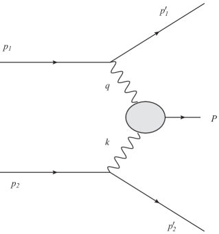
Figure 2: Kinematics for the two-photon pseudoscalar meson production reaction $e^{+}e^{-}\rightarrow e^{+}e^{-}P$.

The cross-section for $e^{+}e^{-}\rightarrow e^{+}e^{-}P$ is given by

$$\sigma=\frac{1}{2}\frac{\alpha^{2}}{(2\pi)^{4}}\frac{1}{s}\int d^{4}q~{}\delta\left(p_{1}.q+\tfrac{1}{2}Q^{2}\right)\int d^{4}k~{}\delta\left(p_{2}.k+\tfrac{1}{2}K^{2}\right)\frac{1}{Q^{4}K^{4}}\\ \times L^{\mu\nu}(p_{1},h_{1};q)M^{\dagger}_{\mu\lambda}(q,k)M_{\nu\rho}(q,k)L^{\lambda\rho}(p_{2},h_{2};k)~{}2\pi\delta(2\nu-Q^{2}-K^{2}-m_{P}^{2})\ ,$$ (52)

where

$$M_{\mu\lambda}(q,k)=-i\epsilon_{\mu\lambda\alpha\beta}q^{\alpha}k^{\beta}g_{P\gamma^{*}\gamma^{*}}(Q^{2},K^{2})$$ (53)

is defined in terms of the off-shell transition functions. This is related to the inclusive cross-section (12) by the optical theorem, which for the specific meson final state $P$ implies the substitution

$$4\pi\alpha K^{4}\operatorname{Im}T_{\mu\nu\lambda\rho}\rightarrow\frac{1}{2}M^{\dagger}_{\mu\lambda}(q,k)M_{\nu\rho}(q,k)~{}2\pi\delta\left((q+k)^{2}-m_{P}^{2}\right)\ .$$ (54)

Notice that in deriving (12) no use has been made of the conventional ‘equivalent photon’ formalism (see, e.g. refs. [15, 16] and no assumption has been made that the target photon is quasi-real. This is essential if we are to measure transition functions covering the whole range of values of $K^{2}$.

We can evaluate the integrand in this expression for the cross-section in the same way as in section 2. Defining the symmetric part of the leptonic tensor of (8) as $L^{S}_{\mu\nu}(p_{1},q)$, we find

$$L_{S}^{\mu\nu}(p_{1},q)M^{\dagger}_{\mu\lambda}(q,k)M_{\nu\rho}(q,k)L_{S}^{\lambda\rho}(p_{2},k)\\ =\Big{[}4J^{-2}+4Q^{2}K^{2}\Big{(}\left(\nu\nu_{e}-\tfrac{1}{4}Q^{2}K^{2}\right)-\nu_{e}^{2}+\left(\nu\bar{\nu}_{e}-\tfrac{1}{4}Q^{2}K^{2}\right)-\bar{\nu}_{e}^{2}-\tfrac{1}{2}\left(\nu^{2}-Q^{2}K^{2}\right)\Big{)}\Big{]}\\ \times~{}|g_{P\gamma^{*}\gamma^{*}}|^{2}$$ (55)

where $J$ is the Jacobian factor in (19). Substituting for $J$, and after reorganising terms on the r.h.s, we find the comparatively simple expression:

$$\left[4\left(s\nu-2\nu_{e}\bar{\nu}_{e}\right)^{2}-4Q^{2}K^{2}\left(\left(s+\tfrac{1}{2}\nu-\nu_{e}-\bar{\nu}_{e}\right)^{2}+\tfrac{1}{4}(\nu^{2}-Q^{2}K^{2})\right)\right]|g_{P\gamma^{*}\gamma^{*}}|^{2}\ .$$ (56)

We recognise the first term here as that previously found in (20), which encodes the dependence on the azimuthal scattering angle $\phi$. To determine the polarization asymmetry of the cross-section, we also require the contribution of the antisymmetric part of the leptonic tensor:

$$L_{A}^{\mu\nu}(p_{1},q)M^{\dagger}_{\mu\lambda}(q,k)M_{\nu\rho}(q,k)L_{A}^{\lambda\rho}(p_{2},k)\\ =-4Q^{2}K^{2}(\nu-2\nu_{e})(\nu-2\bar{\nu}_{e})~{}|g_{P\gamma^{*}\gamma^{*}}|^{2}\ .$$ (57)

Putting all this together, we find the following formula relating the differential cross-section for the exclusive production reaction $e^{+}e^{-}\rightarrow e^{+}e^{-}P$ and the off-shell pseudoscalar meson transition functions $g_{P\gamma*\gamma*}(Q^{2},K^{2})$:

$$\frac{d^{2}\sigma(h_{1},h_{2})}{dQ^{2}dK^{2}} =\frac{\alpha^{2}}{(2\pi)^{2}}\frac{1}{s^{2}Q^{4}K^{4}}\int_{0}^{\infty}d\nu_{e}\int_{0}^{\infty}d\bar{\nu}_{e}\int_{0}^{\infty}d\nu~{}\delta\left(\nu-\tfrac{1}{2}(Q^{2}+K^{2}+m_{P}^{2})\right)~{}J$$

$$\times\bigg{[}(s\nu-2\nu_{e}\bar{\nu}_{e})^{2}-Q^{2}K^{2}\Big{(}(s+\tfrac{1}{2}\nu-\nu_{e}-\bar{\nu}_{e})^{2}+\tfrac{1}{4}(\nu^{2}-Q^{2}K^{2})^{2}$$

$$\hskip 85.35826pt~{}~{}-h_{1}h_{2}(\nu-2\nu_{e})(\nu-2\bar{\nu}_{e})\Big{)}\bigg{]}~{}|g_{P\gamma^{*}\gamma^{*}}(Q^{2},K^{2})|^{2}\ .$$ (58)

This shows clearly how the off-shell transition functions $g_{P\gamma^{*}\gamma^{*}}(Q^{2},K^{2})$, for the full range of $Q^{2}$ and $K^{2}$, may be extracted from the exclusive differential cross-section. Notice that in this case, where the produced hadron is a pseudoscalar, there is only a single transition function (see eq.(53)) and so no extra information is obtained from the polarization asymmetry of the cross-section. The transition functions can therefore be obtained from an $e^{+}e^{-}$ collider running even with unpolarized beams, as was the case with BABAR. This is not true of higher-spin mesons, where knowing the polarized cross-sections analogous to (58) will yield valuable new information. This is especially relevant to $\gamma^{*}\gamma^{*}\rightarrow\gamma^{*}\gamma^{*}$ scattering, as discussed below.

Determining the $\pi,\eta,\eta^{\prime}$ transition functions in this way will complement other low-energy experimental studies of $\eta$ and $\eta^{\prime}$ physics, and add to our understanding of other processes such as $\eta(\eta^{\prime})\rightarrow V\gamma$, where $V=\rho,\omega,\phi$ and vector meson dominance can be tested, or $\eta^{\prime}(\eta)\rightarrow\pi^{+}\pi^{-}\gamma$. For our purposes, it will also add to the usefulness of the set of identities (50). An independent, direct measurement of the off-shell transition functions $g_{P\gamma^{*}\gamma^{*}}(Q^{2},K^{2})$ will allow the form factors $F^{r}(K^{2})$ to be determined and used as input into the $g_{1}^{\gamma}(x,Q^{2};K^{2})$ sum rule. It will also clarify the role of the anomalous gluonic term in (50) and provide indirect experimental information on the gluon topological susceptibility in QCD.

Here, we are primarily interested in $\gamma^{*}\gamma^{*}$ reactions where the target photon is off-shell and both electrons are tagged (see also [46]). This complements the extensive programme of $\gamma^{*}\gamma$, single-tagged, scattering off quasi-real photons which can also be carried out at Super-B [47]. In addition to $\gamma^{*}\gamma\rightarrow P$ at high $Q^{2}$, which is interpreted [48] in terms of meson distribution amplitudes, there is considerable interest in $\gamma^{*}\gamma\rightarrow\pi\pi,\rho\rho$, etc. [16, 49, 50] which can be interpreted in terms of generalised distribution amplitudes (GDAs), related to the GPDs used to analyse deeply-virtual Compton scattering and the angular momentum decomposition of the nucleon. Reactions producing hybrid mesons [51] are also of interest.

(iii)  Light-by-light scattering:

Light-by-light scattering is a fundamental quantum process, interesting both in its own right and because it arises theoretically in the calculation of the anomalous magnetic moment $g-2$ of the muon. Indeed, the hadronic contribution to the light-by-light contribution is currently the major theoretical uncertainty, which in turn constrains the interpretation of any anomalies in the muon $g-2$ as a signal of new physics beyond the standard model [24].

The imaginary part of the light-by-light scattering amplitude is related via the optical theorem to the related process of $\gamma\gamma$ fusion. As discussed above, cross-sections for $\gamma^{*}\gamma^{*}\rightarrow X~{}{\rm hadrons}$ can be readily measured in $e^{+}e^{-}$ colliders and a high-luminosity, polarized machine such as Super B is ideally suited for this purpose.

Labelling the photon helicities by $\lambda_{1}$,$\lambda_{2}$, the imaginary part of the virtual light-by-light forward scattering amplitude is written (compare eq.(54)) as

$$\operatorname{Im}M_{(\lambda_{1})(\lambda_{2}),(\lambda^{\prime}_{1})(\lambda^{\prime}_{2})}(q,k)=\frac{1}{2}\sum_{X}\int d\Gamma_{X}~{}(2\pi)^{4}\delta(q+k-p_{X})~{}\\ {\cal M}^{\dagger}_{(\lambda_{1})(\lambda_{2})}(q,k;p_{X}){\cal M}_{(\lambda^{\prime}_{1})(\lambda^{\prime}_{2})}(q,k;p_{X})\ ,$$ (59)

where ${\cal M}_{(\lambda_{1})(\lambda_{2})}(q,k;p_{X})$ is the amplitude for $\gamma^{*}(q;\lambda_{1})+\gamma^{*}(k;\lambda_{2})\rightarrow X(p_{X})$, with $X$ denoting a hadronic state and $d\Gamma_{X}$ the corresponding phase space measure. There are a total of eight independent helicity amplitudes in $\operatorname{Im}M_{(\lambda_{1})(\lambda_{2}),(\lambda^{\prime}_{1})(\lambda^{\prime}_{2})}$, which can be related to the cross-sections for $\gamma^{*}\gamma^{*}\rightarrow X$ with different photon helicities and spins of the hadronic state $X$. These are listed in full in ref.[45], together with the corresponding dispersion relations. In particular, to make contact with the results above, if the hadron is a pseudoscalar meson $P$ then the only non-vanishing scattering amplitudes ${\cal M}_{(\lambda_{1})(\lambda_{2})}$ are those with the photons transversely polarized in the same sense, and we can show from the definition in footnote 8 that

$${\cal M}_{++}(q,k)=-{\cal M}_{--}(q,k)=-4\pi\alpha\left(\nu^{2}-Q^{2}K^{2}\right)^{\tfrac{1}{2}}~{}g_{P\gamma^{*}\gamma^{*}}(Q^{2},K^{2})\ .$$ (60)

The other light-by-light helicity amplitudes $M_{(\lambda_{1})(\lambda_{2})(\lambda^{\prime}_{1})(\lambda^{\prime}_{2})}(q,k)$ are similarly determined from measurements of the $\gamma^{*}\gamma^{*}$ amplitudes ${\cal M}_{(\lambda_{1})(\lambda_{2})}(q,k;p_{X})$, which are in turn measured from the exclusive $e^{+}e^{-}\rightarrow e^{+}e^{-}X$ cross-sections for different hadronic states and electron polarizations.

So once more we see from a different perspective the importance of measuring the off-shell meson transition functions. In particular, we want to highlight the close connection between the form factors describing low-energy pseudoscalar meson decays, the light-by-light scattering amplitudes relevant to the muon $g-2$, and the first moment sum rule for the photon structure functions $g_{1}^{\gamma}(x,Q^{2};K^{2})$. This whole rich spectrum of complementary QCD phenomena would be experimentally accessible given a dedicated programme of two-photon physics at Super B.

5 QCD at Super-B

In this final section, we use the design parameters of Super-B to investigate the feasibility of the programme of two-photon QCD physics described above, with particular focus on the possibility of verifying the first moment sum rule for $g_{1}^{\gamma}(x,Q^{2};K^{2})$. Here, the key issues concern the luminosity, beam polarization and the possibility of tagging the target electron.

The first issue is whether the luminosity is sufficiently high to allow $g_{1}^{\gamma}(x,Q^{2};K^{2})$ to be measured from the polarization asymmetry of the differential cross section, according to eq.(16). The total, polarization averaged, cross-section $\sigma$ is expressed in terms of the photon structure functions $F_{2}^{\gamma}(x,Q^{2};K^{2})$ and $F_{L}^{\gamma}(x,Q^{2};K^{2})$ by

$$\sigma={\alpha^{3}}\int_{0}^{\infty}\frac{dQ^{2}}{Q^{4}}\int_{0}^{1}\frac{dx_{e}}{x_{e}}\int_{0}^{\infty}\frac{dK^{2}}{K^{2}}\int_{x_{e}}^{1}\frac{dx}{x}~{}\frac{x_{e}}{x}P_{\gamma e}\left(\frac{x_{e}}{x}\right)\\ \times\left[F_{2}^{\gamma}\left(1-\frac{Q^{2}}{x_{e}s}+\frac{1}{2}\frac{Q^{4}}{x_{e}^{2}s^{2}}\right)-\frac{1}{2}F_{L}^{\gamma}\frac{Q^{4}}{x_{e}^{2}s^{2}}\right]$$ (61)

where $P_{\gamma e}(z)=(1+(1-z)^{2})/z$. To find an initial estimate, we again work to leading order in $Q^{2}/x_{e}s$, so retain only the $F_{2}^{\gamma}$ contribution. The polarization asymmetry is given by (14),

$$\Delta\sigma={\alpha^{3}\over s}\int_{0}^{\infty}{dQ^{2}\over Q^{2}}\int_{0}^{1}{dx_{e}\over x_{e}}\int_{0}^{\infty}{dK^{2}\over K^{2}}\int_{x_{e}}^{1}{dx\over x}~{}\Delta P_{\gamma e}\left({x_{e}\over x}\right)~{}g_{1}^{\gamma}(x,Q^{2};K^{2})~{}\Big{(}1-{Q^{2}\over 2x_{e}s}\Big{)}\ .$$ (62)

To estimate these cross-sections, we use the dominant contribution to the moments, viz.

$$\int_{0}^{1}dx~{}x^{n-1}F_{2}^{\gamma}(x,Q^{2};K^{2}) \simeq{\alpha\over 4\pi}a_{n+1}\log\frac{Q^{2}}{\Lambda^{2}}\ ,\hskip 28.45274ptn\geq 1,~{}{\rm odd}$$

$$\int_{0}^{1}dx~{}x^{n-1}g_{1}^{\gamma}(x,Q^{2};K^{2}) \simeq{\alpha\over 4\pi}b_{n+1}\log\frac{Q^{2}}{\Lambda^{2}}\ ,\hskip 28.45274ptn\geq 3,~{}{\rm odd}\ ,$$ (63)

where $a_{n+1},b_{n+1}$ are known [52, 53]. Taking the inverse Mellin transform, we deduce

$$F_{2}^{\gamma} \simeq\frac{\alpha}{4\pi}a(x)\log\frac{Q^{2}}{\Lambda^{2}}$$

$$g_{1}^{\gamma} \simeq\frac{\alpha}{4\pi}b(x)\log\frac{Q^{2}}{\Lambda^{2}}\ ,$$ (64)

where numerically $a(x)$ and $b(x)$ are approximately constant, with $1.2<a(x)<1.6$ for $0.3<x<0.9$. For the estimates below, we take $a(x)\simeq\bar{a}\simeq 1.5$ with the same value for $b(x)\simeq\bar{b}$. Placing upper and lower limits on the integrations over $Q^{2}$, $K^{2}$, $x_{e}$ and $x$, we therefore find [7]:

$$\sigma \simeq\frac{\alpha^{4}}{2\pi}\bar{a}\frac{1}{Q^{2}_{min}}\log\frac{Q^{2}_{min}}{\Lambda^{2}}\log\frac{K^{2}_{\max}}{K^{2}_{min}}\log\frac{x_{e}^{max}}{x_{e}^{min}}\log\frac{x_{max}}{\langle x_{e}\rangle}$$

$$\Delta\sigma \simeq\frac{\alpha^{4}}{2\pi}\bar{b}\frac{1}{s}\log\frac{Q^{2}_{max}}{Q^{2}_{min}}\log\frac{\langle Q^{2}\rangle}{\Lambda^{2}}\log\frac{K^{2}_{\max}}{K^{2}_{min}}\log\frac{x_{e}^{max}}{x_{e}^{min}}\log\frac{x_{max}}{\langle x_{e}\rangle}\ ,$$ (65)

where $\langle Q^{2}\rangle$ is the geometric mean of $Q^{2}_{max}$ and $Q^{2}_{min}$, and similarly for $x_{e}$. The ratio $\Delta\sigma/\sigma$ is therefore

$$\frac{\Delta\sigma}{\sigma}\simeq\frac{1}{2}\frac{Q^{2}_{min}}{s}\log\frac{Q^{2}_{max}}{Q^{2}_{min}}\left[1+\log\frac{Q^{2}_{max}}{\Lambda^{2}}\left(\log\frac{Q^{2}_{min}}{\Lambda^{2}}\right)^{-1}\right]\ .$$ (66)

The experimental cuts are chosen as follows. We take $K^{2}_{min}\simeq 0.1~{}{\rm GeV}^{2}$ and $K^{2}_{max}\simeq 2~{}{\rm GeV}^{2}$, above the non-perturbatively interesting region $K^{2}\sim m_{\rho}^{2}$ where the first moment of $g_{1}^{\gamma}(x,Q^{2};K^{2})$ rises from 0 to its asymptotic value. For the Bjorken variables, we choose $\nu_{e}^{max}=\nu_{max}\simeq s/2$ from (4), and $\nu_{e}^{min}=\nu_{min}\simeq Q^{2}_{min}/2$ to ensure $x_{e}$ and $x$ greater than zero, while $Q^{2}_{max}\simeq s/2$. Finally, the lower cut $Q^{2}_{min}$ is retained as a free parameter which we will vary in order to optimise the asymmetry $\Delta\sigma/\sigma$ while retaining a sufficiently high total cross-section.

With these cuts, we find [7, 9]

$$\sigma\simeq 10^{-9}\frac{1}{Q^{2}_{min}}\log\frac{Q^{2}_{min}}{\Lambda^{2}}\left(\log\frac{s}{Q^{2}_{min}}\right)^{2}\ ,$$ (67)

while

$$\frac{\Delta\sigma}{\sigma}\simeq\frac{1}{2}\frac{Q^{2}_{min}}{s}\log\frac{s}{2Q^{2}_{min}}\left[1+\log\frac{s}{2\Lambda^{2}}\left(\log\frac{Q^{2}_{min}}{\Lambda^{2}}\right)^{-1}\right]\ .$$ (68)

Notice in particular the relative $1/s$ supression of the polarization asymmetry. This explains why a moderate energy $e^{+}e^{-}$ collider is best suited to the polarized QCD studies proposed here. The CM energy of B factories such as Super-B, with $\sqrt{s}=10.6~{}{\rm GeV}$, is ideal.

      

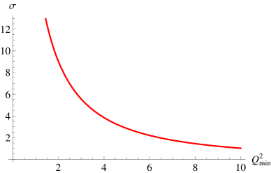
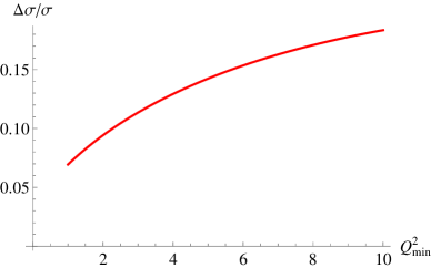
Figure 3: The total cross-section $\sigma$, measured in pb, for the inclusive reaction $e^{+}e^{-}\rightarrow e^{+}e^{-}X$ plotted against the lower cut-off $Q^{2}_{min}$ in ${\rm GeV}^{2}$. The corresponding polarization asymmetry $\Delta\sigma/\sigma$ is shown in the right-hand figure.

In Fig. 3, we plot $\sigma$ (in pb) and $\Delta\sigma/\sigma$ for the Super-B $\sqrt{s}$ over the range of $Q^{2}_{min}$ from 1 to 10 ${\rm GeV}^{2}$. As is clear from the formulae above, we see that as $Q^{2}_{min}$ is increased, the asymmetry $\Delta\sigma/\sigma$ increases, but at the cost of reducing the total cross-section $\sigma$. A reasonable compromise is therefore to take $Q^{2}_{min}\simeq 2~{}{\rm GeV}^{2}$, which gives $\sigma\simeq 10~{}{\rm pb}$ with an asymmetry $\Delta\sigma/\sigma=0.1$.

The extremely high luminosity of Super-B means that this cross-section is sufficient to give a large number of events. The design luminosity is $10^{36}~{}{\rm cm}^{-2}{\rm s}^{-1}$ and ref.[4] quotes a potential annual integrated luminosity $L=12~{}{\rm ab}^{-1}$. With the above choice of the $Q^{2}_{min}$ cut, this corresponds to $N=L\sigma=10^{8}$ events/year, with a 10% polarization asymmetry. To check the statistical significance of this asymmetry, we require $\Delta N/\sqrt{N}\gg 1$ and with these cuts we find $\Delta N/\sqrt{N}=\sqrt{L\sigma}\Delta\sigma/\sigma\simeq 10^{3}$. Of course, to measure the first moment sum rule for $g_{1}^{\gamma}(x,Q^{2};K^{2})$ we need to distribute these events into sufficient $Q^{2}$ and $K^{2}$ bins, but with such a high event rate even the differential cross-section $d^{2}\Delta\sigma/dQ^{2}dK^{2}$ should be easily measurable with high precision.

The second main accelerator issue is polarization. In order to measure the polarization asymmetry, both beams need to be polarized. At present, the Super-B design only envisages polarizing the low-energy beam, as required for example for $\tau$ polarization studies, but there appears to be no insurmountable technical obstacle to polarizing both beams given sufficient physics motivation, which we believe an extensive programme of polarized QCD physics provides.

The polarization scheme designed for Super-B is described in detail in chapter 16 of ref.[4] (see also [6]). It involves the continuous injection of transversely polarized electrons into the low-energy ring (LER) and subsequently use of an arrangement of spin rotator solenoids to bring the electron polarization into longitudinal mode at the intersection region. The LER is chosen simply because the strength of the solenoids scales with energy. The design estimates that polarization efficiencies in excess of 70% at high luminosity can be sustained.

Finally, to measure the $K^{2}$ dependence of $g_{1}^{\gamma}(x,Q^{2};K^{2})$ in detail in the dynamically interesting region $K^{2}<1.5~{}{\rm GeV}^{2}$, we need to tag the ‘target’ electron at sufficiently small angles, since $K^{2}=4E_{2}E_{2}^{\prime}\sin^{2}(\theta_{2}/2)$. Ideally, we would like to be able to detect the electron at very small scattering angles $\theta_{2}$, to allow for small values of $K^{2}$ to be measured for comparatively large energies $E_{2}^{\prime}$. This raises the critical issue of detector acceptance.

The Super-B detector [5], which is based on a major upgrade of BABAR, can detect particles with angles greater than 300 mrad to the beam direction (see Fig. 1 of ref.[5] for an overview sketch of the planned detector). It is not clear whether it would be possible to add small angle detectors capable of tagging an electron at angles around 50-100 mrad [44] to the proposed design. However, as we now show, the comparatively modest beam energy of Super-B (taking $E_{2}=4.18~{}{\rm GeV}$ from the low-energy ring) means that even the detector acceptance of 300 mrad will in fact allow the target electron to be tagged with the required values of $K^{2}$ while satisfying the kinematical constraints for deep-inelastic scattering.

      

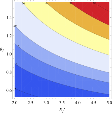
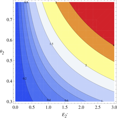
Figure 4: The left-hand figure (4a) shows a contour plot of $Q^{2}$ from 5 to 60 ${\rm GeV}^{2}$ for a range of electron scattering energies and angles $E_{1}^{\prime}$ and $\theta_{1}^{\prime}$. The analogous contour plot for $K^{2}$ is shown in the right-hand figure (4b). This shows how the important region $0.2<K^{2}<1.5~{}{\rm GeV}^{2}$ is accessible with target electron scattering energy in the range $0.5<E_{2}^{\prime}<2.5~{}{\rm GeV}^{2}$ with angle $\theta_{2}$ greater than the detector acceptance 300 mrad.

The dependence of $Q^{2}$ on $E_{1}^{\prime}$ and $\theta_{1}^{\prime}$, and the dependence of $K^{2}$ on $E_{2}^{\prime}$ and $\theta_{2}^{\prime}$, are given in eq.(4) and illustrated in the contour plots in Fig. 4. The $Q^{2}$ plot shows that the full range of desired values from the optimal cut $Q^{2}_{min}\simeq 2~{}{\rm GeV}^{2}$ up to $Q^{2}_{max}\simeq s/2$ can be easily realised for scattering angles $\theta_{1}^{\prime}>300~{}{\rm mrad}$ and energies $E_{1}^{\prime}$ from 2-5 GeV. The required range $K^{2}\lesssim 1.5~{}{\rm GeV}^{2}$ is shown by the series of curves in the lower left of the contour plot Fig. 4b. This shows that the whole range $0.2<K^{2}<1.5~{}{\rm GeV}^{2}$ can be covered by tagging the electron with $300~{}{\rm mrad}<\theta_{2}^{\prime}<\pi/4$ and energy $E_{2}^{\prime}$ in the range $0.5<E_{2}^{\prime}<2.5~{}{\rm GeV}$. We conclude that, coupled with the large number of events in this range guaranteed by the ultra-high luminosity, the Super-B detector will indeed be able to cover the range of $K^{2}$ and $Q^{2}$ necessary to measure the $g_{1}^{\gamma}(x,Q^{2};K^{2})$ sum rule.

      

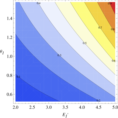
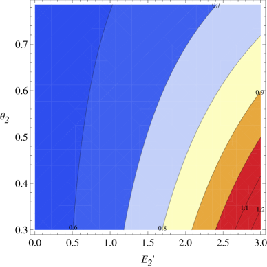
Figure 5: The left-hand figure (5a) shows a contour plot of $x_{e}=Q^{2}/2\nu_{e}$ over a range of $E_{1}^{\prime}$ and $\theta_{1}$. The right-hand figure (5b) shows the corresponding plot for $x=Q^{2}/2\nu$ as a function of $E_{2}^{\prime}$ and $\theta_{2}$ for values $E_{1}^{\prime}=4.5~{}{\rm GeV}$, $\theta_{1}=\pi/3$. Satisfying the constraint $x<1$ near the detector acceptance angle $\theta_{2}\simeq 300~{}{\rm mrad}$ imposes an upper bound $E_{2}^{\prime}<2.5~{}{\rm GeV}$.

We also need to check the constraints on the remaining DIS variables. From the derivation of the cross-sections involving $g_{1}^{\gamma}$, we require the hierarchy $\nu_{e}>\nu>\tfrac{1}{2}(Q^{2}+K^{2})$, since clearly the hadronic invariant momentum $W^{2}>0$, as well as $x_{e}=Q^{2}/2\nu_{e}<1$ and $x=Q^{2}/2\nu<1$. Expressions for $\nu_{e}$ and $\nu$ in terms of the scattering energies and angles are given in eq.(4), and we also have the following useful relation

$$\nu_{e}-\nu=E_{2}^{\prime}\Big{[}E_{1}(1+\cos\theta_{2})-E_{1}^{\prime}\big{(}1+\cos(\theta_{1}-\theta_{2})+\sin\theta_{1}\sin\theta_{2}(1-\cos\phi)\big{)}\Big{]}$$ (69)

The condition $x_{e}<1$ is satisfied provided only that $E_{1}^{\prime}$ is not too big, and from Fig. 5a we see that $E_{1}^{\prime}\lesssim 5~{}{\rm GeV}$ is sufficient. The condition $x<1$ is however much more stringent and places an important upper bound on $E_{2}^{\prime}$, which reduces as the maximum value of $E_{1}^{\prime}$ increases. From Fig. 5b we see that to maintain $x<1$ with $E_{2}^{\prime}\lesssim 2.5~{}{\rm GeV}$ at $\theta_{2}=300~{}{\rm mrad}$, we have to cut off $E_{1}^{\prime}$ and $\theta_{1}^{\prime}$ at around 4.5 GeV and $\pi/3$ respectively, corresponding to $Q^{2}\simeq 30~{}{\rm GeV}^{2}$. This is nevertheless a perfectly acceptable upper cut-off on $Q^{2}$ for the DIS analysis. This maximum value of $E_{2}^{\prime}$ is necessary to optimise the available data in the required low $K^{2}$ region, as shown above. We can then show, using (69) and numerical plots, that $\nu_{e}>\nu$ provided $\theta_{2}$ is below an upper bound of around $\pi/3$, so we confirm that the full hierarchy $\nu_{e}>\nu>\tfrac{1}{2}(Q^{2}+K^{2})$ holds for the range of variables already determined.

In summary, all the kinematical constraints for the DIS analysis of the first moment sum rule for $g_{1}^{\gamma}(x,Q^{2};K^{2})$ are satisfied with scattering angles and energies allowing measurements of $Q^{2}$ in the range $2<Q^{2}<30~{}{\rm GeV}^{2}$ with $K^{2}$ satisfying $0.2<K^{2}<1.5~{}{\rm GeV}^{2}$, provided we tag both electrons with $2\lesssim E_{1}^{\prime}\lesssim 4.5~{}{\rm GeV}$, $\theta_{1}\lesssim\pi/3$ and $0.5<E_{2}^{\prime}<2.5~{}{\rm GeV}$, $\theta_{2}\lesssim\pi/4$ with both electrons scattered within the detector acceptance $\theta_{1},\theta_{2}>300~{}{\rm mrad}.$

Finally, we discuss briefly the prospects for measuring exclusive processes at Super-B, such as the two-photon production of pseudoscalar mesons through $e^{+}e^{-}\rightarrow e^{+}e^{-}P$. The kinematics relating the invariants $Q^{2},K^{2},\nu_{e}$ and $\bar{\nu}_{e}$ to the observed electron scattering angles and energies is given in eq.(4) as described above. In the exclusive case, however, $\nu$ is fixed by the constraint $W^{2}=m_{P}^{2}$, while now the DIS constraints on $Q^{2}$ and $\nu_{e}$ are no longer relevant. Tagging both electrons allows the off-shell meson transition functions $g_{P\gamma^{*}\gamma^{*}}(Q^{2},K^{2})$ to be measured for essentially arbitrary values of $Q^{2}$ and $K^{2}$, including very soft photons with $Q^{2}$ and/or $K^{2}$ down to around $0.2~{}{\rm GeV}^{2}$, limited only by the detector acceptance. Knowledge of these transition functions will feed directly into eqs.(50) for the non-perturbative form factors characterising the first moment of $g_{1}^{\gamma}(x,Q^{2};K^{2})$.

The differential cross-section for $e^{+}e^{-}\rightarrow e^{+}e^{-}P$ was derived in eq.(58). As already explained, since $\gamma^{*}\gamma^{*}\rightarrow P$ for pseudoscalar $P=\pi,\eta,\eta^{\prime}$ is determined by a single form factor, the transition functions can be obtained with unpolarized beams. The polarization asymmetry would of course give new information for two-photon production of higher-spin mesons which are characterised by more than one form factor. Note also from (58) that in the exclusive case, the polarization asymmetry of the differential cross-section is suppressed by a double factor $O(Q^{2}K^{2}/s^{2})$ compared to the single suppression $O(Q^{2}/s)$ for the inclusive process. The ultra-high luminosity of Super-B will allow a much-improved study of the off-shell transition functions $g_{P\gamma^{*}\gamma^{*}}(Q^{2},K^{2})$ with both $Q^{2}$ and $K^{2}$ specified compared to the existing data from CELLO [19], CLEO [20] and BABAR [21, 22, 23].

In conclusion, we have shown how the unique combination of moderate energy, polarization and ultra-high luminosity, together with its detector capability, means Super-B has the ideal characteristics to support an ambitious programme of two-photon QCD physics. This includes, but is not limited to, the investigation of pseudoscalar meson transition functions, with their relevance to the muon $g-2$, and the photon structure functions $g_{1}^{\gamma}(x,Q^{2};K^{2})$ and $g_{2}^{\gamma}(x,Q^{2};K^{2})$, including the potential to make the first experimental measurement of the first moment sum rule for $g_{1}(x,Q^{2};K^{2})$. This will give direct experimental input into many interesting theoretical issues in QCD, including chiral symmetry breaking, $U(1)_{A}$ dynamics, gluon topology and anomalous chiral symmetry. All this provides strong motivation for including polarized two-photon QCD physics as an important element of the research programme planned for Super-B.

*******

I would like to thank S. Narison and G. Veneziano for their original collaboration on the photon sum rule and the Theory Division, CERN for hospitality during the course of this work. I am grateful to the U.K. Science and Technology Facilities Council (STFC) for financial support under grant ST/J000043/1.

References

[1]
[2]
M. Bona et al. [SuperB Collaboration],
“SuperB: A High-Luminosity Asymmetric Super Flavor Factory. Conceptual Design Report,”
Pisa, Italy: INFN (2007) 453p. www.pi.infn.it/SuperB/?q=CDR
[arXiv:0709.0451 [hep-ex]]; http://superb.infn.it/home.
[3]
B. O’Leary et al. [SuperB Collaboration],
“SuperB Progress Reports – Physics,”
arXiv:1008.1541 [hep-ex].
[4]
M. E. Biagini et al. [SuperB Collaboration],
“SuperB Progress Reports – The Collider,”
arXiv:1009.6178 [physics.acc-ph].
[5]
E. Grauges et al. [SuperB Collaboration]
“ SuperB Progress Reports – Detector,”
arXiv:1007.4241 [physics.ins-det].
[6]
U. Wienands, Y. Nosochkov, M. Sullivan, W. Wittmer, D. Barber,
M. Biagini, P. Raimondi and I. Koop et al.,
“Polarization in SuperB,”
Conf. Proc. C 100523 (2010) TUPEB029.
[7]
S. Narison, G. M. Shore and G. Veneziano,
Nucl. Phys. B 391 (1993) 69.
[8]
G. M. Shore and G. Veneziano,
Mod. Phys. Lett. A 8 (1993) 373.
[9]
G. M. Shore,
Nucl. Phys. B 712 (2005) 411
[hep-ph/0412192].
[10]
S. D. Bass,
Int. J. Mod. Phys. A 7 (1992) 6039.
[11]
S. D. Bass, S. J. Brodsky and I. Schmidt,
Phys. Lett. B 437 (1998) 417
[hep-ph/9805316].
[12]
K. Sasaki and T. Uematsu,
Phys. Rev. D 59 (1999) 114011
[hep-ph/9812520].
[13]
T. Ueda, T. Uematsu and K. Sasaki,
Phys. Lett. B 640 (2006) 188
[hep-ph/0606267].
[14]
K. Sasaki, T. Ueda and T. Uematsu,
Phys. Rev. D 73 (2006) 094024
[hep-ph/0604130].
[15]
C. Berger and W. Wagner,
Phys. Rept. 146 (1987) 1.
[16]
S. J. Brodsky, T. Kinoshita and H. Terazawa,
Phys. Rev. D 4 (1971) 1532.
[17]
H. Baba, K. Sasaki and T. Uematsu,
Phys. Rev. D 65 (2002) 114018
[hep-ph/0202142].
[18]
G. M. Shore,
Lect. Notes Phys. 737 (2008) 235
[hep-ph/0701171].
[19]
H. J. Behrend et al. [CELLO Collaboration],
Z. Phys. C 49 (1991) 401.
[20]
J. Gronberg et al. [CLEO Collaboration],
Phys. Rev. D 57 (1998) 33
[hep-ex/9707031].
[21]
B. Aubert et al. [BABAR Collaboration],
Phys. Rev. D 80 (2009) 052002
[arXiv:0905.4778 [hep-ex]].
[22]
P. del Amo Sanchez et al. [BABAR Collaboration],
Phys. Rev. D 84 (2011) 052001
[arXiv:1101.1142 [hep-ex]].
[23]
J. P. Lees et al. [BABAR Collaboration],
Phys. Rev. D 81 (2010) 052010
[arXiv:1002.3000 [hep-ex]].
[24]
F. Jegerlehner and A. Nyffeler,
Phys. Rept. 477 (2009) 1
[arXiv:0902.3360 [hep-ph]].
[25]
G. M. Shore and G. Veneziano,
Nucl. Phys. B 381 (1992) 3.
[26]
G. M. Shore,
Nucl. Phys. B 569 (2000) 107
[hep-ph/9908217].
[27]
G. M. Shore,
Nucl. Phys. B 744 (2006) 34
[hep-ph/0601051].
[28]
K. Sasaki,
Phys. Rev. D 58 (1998) 094007
[hep-ph/9803282].
[29]
M. Stratmann,
Nucl. Phys. Proc. Suppl. 82 (2000) 400
[hep-ph/9907467].
[30]
K. Sasaki and T. Uematsu,
Phys. Lett. B 473 (2000) 309
[hep-ph/9911424].
[31]
K. Sasaki and T. Uematsu,
Nucl. Phys. Proc. Suppl. 89 (2000) 162
[hep-ph/0006025].
[32]
J. Kwiecinski and B. Ziaja,
Phys. Rev. D 63 (2001) 054022
[hep-ph/0006292].
[33]
M. Gluck, E. Reya and C. Sieg,
Phys. Lett. B 503 (2001) 285
[hep-ph/0102014].
[34]
H. Baba, K. Sasaki and T. Uematsu,
Phys. Rev. D 68 (2003) 054025
[hep-ph/0307136].
[35]
N. Watanabe, Y. Kiyo and K. Sasaki,
Phys. Lett. B 707 (2012) 146
[arXiv:1110.2625 [hep-ph]].
[36]
J. Kodaira, Y. Yasui and T. Uematsu,
Phys. Lett. B 344 (1995) 348
[hep-ph/9408354].
[37]
H. Burkhardt and W. N. Cottingham,
Annals Phys. 56 (1970) 453.
[38]
S. Wandzura and F. Wilczek,
Phys. Lett. B 72 (1977) 195.
[39]
K. Melnikov and A. Vainshtein,
Phys. Rev. D 70 (2004) 113006
[hep-ph/0312226].
[40]
R. J. Crewther, P. Di Vecchia, G. Veneziano and E. Witten,
Phys. Lett. B 88 (1979) 123
[Erratum-ibid. B 91 (1980) 487].
[41]
H. Leutwyler and A. V. Smilga,
Phys. Rev. D 46 (1992) 5607.
[42]
S. J. Brodsky, T. Kinoshita and H. Terazawa,
Phys. Rev. Lett. 25 (1970) 972.
[43]
S. J. Brodsky, T. Kinoshita and H. Terazawa,
Phys. Rev. Lett. 27 (1971) 280.
[44]
H. Kolanoski and P. M. Zerwas,
“Two Photon Physics,”
in Ali, A., Soeding, P. (eds.): High-Energy Electron-Positron Physics
695-784, and Hamburg DESY – DESY 87-175 (1987).
[45]
V. Pascalutsa, V. Pauk and M. Vanderhaeghen,
Phys. Rev. D 85 (2012) 116001
[arXiv:1204.0740 [hep-ph]].
[46]
B. Pire, M. Segond, L. Szymanowski and S. Wallon,
Phys. Lett. B 639 (2006) 642
[hep-ph/0605320].
[47]
B. Pire, L. Szymanowski and S. Wallon, unpublished note. See also
L. Szymanowski,
http://agenda.infn.it/getFile.py/access?contribId=173&sessionId=21&resId=0& materialId=slides&confId=3352
[48]
S. J. Brodsky and G. P. Lepage,
Phys. Rev. D 24 (1981) 1808.
[49]
M. Diehl, T. Gousset and B. Pire,
Phys. Rev. D 62 (2000) 073014
[hep-ph/0003233].
[50]
P. Achard et al. [L3 Collaboration],
Phys. Lett. B 568 (2003) 11
[hep-ex/0305082].
[51]
I. V. Anikin, B. Pire, L. Szymanowski, O. V. Teryaev and S. Wallon,
Eur. Phys. J. C 47 (2006) 71
[hep-ph/0601176].
[52]
W. A. Bardeen and A. J. Buras,
Phys. Rev. D 20 (1979) 166
[Erratum-ibid. D 21 (1980) 2041].