MOA-2010-BLG-073L: An M-Dwarf with a Substellar Companion at the Planet/Brown Dwarf Boundary

Abstract

We present an analysis of the anomalous microlensing event, MOA-2010-BLG-073, announced by the Microlensing Observations in Astrophysics survey on 2010-03-18. This event was remarkable because the source was previously known to be photometrically variable. Analyzing the pre-event source lightcurve, we demonstrate that it is an irregular variable over time scales $>$200 d. Its dereddened color, $(V-I)_{S,0}$, is 1.221$\pm$0.051 mag and from our lens model we derive a source radius of 14.7$\pm$1.3 $R_{\odot}$, suggesting that it is a red giant star. We initially explored a number of purely microlensing models for the event but found a residual gradient in the data taken prior to and after the event. This is likely to be due to the variability of the source rather than part of the lensing event, so we incorporated a slope parameter in our model in order to derive the true parameters of the lensing system. We find that the lensing system has a mass ratio of $q$=0.0654$\pm$0.0006. The Einstein crossing time of the event, $t_{\rm{E}}$=44.3$\pm$0.1 d, was sufficiently long that the lightcurve exhibited parallax effects. In addition, the source trajectory relative to the large caustic structure allowed the orbital motion of the lens system to be detected. Combining the parallax with the Einstein radius, we were able to derive the distance to the lens, $D_{L}$=2.8$\pm$0.4 kpc, and the masses of the lensing objects. The primary of the lens is an M-dwarf with $M_{L,1}$=0.16$\pm$0.03 $M_{\odot}$ while the companion has $M_{L,2}$=11.0$\pm$2.0 $M_{\rm{J}}$, putting it in the boundary zone between planets and brown dwarfs.

1 Introduction

The mass function of individual compact objects (brown dwarfs and planets) in the Galaxy remains poorly understood, particularly at the low-mass end. Brown dwarfs (BD) are commonly defined as objects with masses between the deuterium and hydrogen burning limits (DBL and HBL, respectively) but these can be hard to detect, being intrinsically faint and fading further as they cool over time. Below the DBL, the mass function for individual objects is even more poorly measured. Unbound, free-floating objects of planetary mass have been discovered via direct imaging of clusters (for example in $\sigma$ Orionis (Béjar et al., 2012)) and in the field (e.g. the 6–25 $M_{\rm{J}}$ object reported by Kirkpatrick et al. (2006)). Sumi et al. (2011) reported a population of planets which are either unbound or at very wide separations, discovered when their gravity caused short timescale microlensing events.

At least partially as a result of these poor constraints the origin of low-mass compact objects remain unclear. Although traditionally thought of as separate classes of objects, planets and brown dwarfs form a continuous scale of mass and are best distinguished by the circumstances of their formation (Burrows et al., 2001; Chabrier et al., 2005; Sahlmann et al., 2010; Chabrier et al., 2011). Planets form in disks of material orbiting a protostellar object and may subsequently migrate to different period orbits. Brown dwarfs on the other hand, are considered to be the extreme low mass end of the star formation process by fragmentation of locally over dense cores caused by turbulence in a cloud (Chabrier et al., 2011), which can themselves form protoplanetary disks (Klein et al., 2003; Scholz et al., 2006). This mechanism may also produce objects of a few Jupiter masses. For a recent review, see Luhman (2012).

The mass function of free-floating low-mass objects is likely to be different from those bound to stars. Marcy & Butler (2000) identified a paucity of BDs orbiting close ($<$3 AU) to their host stars, a region where Jovian-mass planets are commonly found. This “brown dwarf desert” may represent the gap between the largest objects that can form in protoplanetary disks and the smallest objects that can concurrently collapse/condense next to a star.

Two different theories have been proposed to explain the formation of Jovian planets in disks (for a review, see Zhou et al. (2012)). The core accretion model predicts planets form from protoplanetary cores, growing up to tens of Jupiter masses (Mordasini et al., 2009; Baraffe et al., 2010, e.g.) but predicts few giant planets around M-dwarfs. Higher mass stars are thought to have disks with enhanced surface densities which allow the cores to grow more rapidly (Laughlin et al., 2004), as do disks with a high fraction of dust, leading to enhanced planet formation around high metallicity stars (Ida & Lin, 2004). Alternatively, the model of planet formation via gravitational instabilities in the disk (Boss, 2006, e.g.) tends to favor the formation of more massive planets, in generally wider orbits.

A number of lines of evidence support the core accretion theory. There is a well-established correlation of increasing planet frequency with stellar metallicity (Santos, Israelian & Mayor, 2001; Fischer & Valenti, 2005; Maldonado et al., 2012). The results of radial velocity surveys imply there is a derth of M-dwarf stars with massive, close-in planets. In part, this reflects an observational bias against these faint objects but the sample is sufficiently large that a real statistical trend is emerging (Cumming et al., 2008; Johnson et al., 2010; Bonfils et al., 2011), for companions with $P<2000$ d. Recent spectroscopic and Kepler results have confirmed the prediction of a rapid increase in frequency for planets with small radii (down to 2$R_{\oplus}$) and $P<50$ d for all spectral types, and found that these small planets are several times more common around stars of late spectral type (Bonfils et al., 2011; Howard et al, 2012).

However, the core accretion model has difficulty forming massive planets at large orbital radii and such systems have been discovered, for example HR 8799 (Marois et al., 2008). Furthermore, a number of planets have been found orbiting M-dwarf hosts at larger orbital separations, for example Dong et al. (2006); Forveille et al. (2011); Batista et al. (2011). These systems may instead form through gravitational instability in the disk, which can account for companions up to several Jupiter masses around M-dwarfs (Boss, 2006).

To better understand the formation mechanisms of heavy substellar companions in bound systems we need to trace the distributions of the physical and orbital properties (such as mass ratio, orbital separation, occurrence frequency) of a significant number of systems. Yet relatively few bound brown dwarf companions have been reported, despite their being easy to detect at close orbital separations (the “brown dwarf desert”).

Microlensing offers a complementary window onto BD and planet formation by probing for cooler companions of all masses in orbital radii between $\sim$0.2 – 10 AU, separations which are difficult or time consuming to explore by other methods (Shin et al., 2012a). It can probe the companion mass function down to M- and brown dwarf hosts, and is sensitive to companions from nearly equal mass down to terrestrial masses.

Sixteen systems have been published to date, and thanks to large-scale galactic lensing surveys and efficient follow-up, each season’s Bulge observing campaign is now producing a regular yield of new discoveries (e.g. Bachelet et al. (2012); Yee et al. (2012); Miyake et al. (2012)). Of these 16 companions, 3 are giant planets orbiting M-dwarf stars: OGLE-2005-BLG-071Lb, a 3.8 $M_{\rm{J}}$ planet (Dong et al., 2009), MOA-2009-BLG-0387Lb, with $M_{P}$=2.5 $M_{\rm{J}}$ planet (Batista et al., 2011) and MOA-2011-BLG-293Lb, which hosts a 2.4 $M_{\rm{J}}$ companion (Yee et al., 2012).

Here we present the newly discovered system, MOA-2010-BLG-073L (catalog MOA-2010-BLG-073L), an M-dwarf star with a companion whose mass is close to the deuterium burning limit of $\sim$12.6 $M_{\rm{J}}$. The discovery and follow-up observations are described in § 2 and we discuss the variability of the source star in § 3. We describe our analysis in § 4, from which we derive the physical properties of the lens in § 5. Finally, we discuss our findings in § 6.

2 Observations

The microlensing event, MOA-2010-BLG-073 (catalog MOA-2010-BLG-073), was first announced by the Microlensing Observations in Astrophysics (MOA, Bond et al. (2001); Sumi et al. (2003) on the 1.8 m telescope at Mt. John Observatory, New Zealand) survey on 2010-03-18. A background source star in the Galactic Bulge, $\alpha$=18:10:11.342, $\delta$=-26:31:22.544 (J2000.0), previously having a mean baseline magnitude of $I\sim$16.5 mag, was discovered to be rising smoothly in brightness consistent with a point-source, point-lens (PSPL) microlensing event. However, on 2010-05-03 the event was found to show an anomalous brightening of $\sim$ 0.5 mag and an alert was issued (K. Furusawa, private comm.).

Microlensing follow-up teams worldwide – RoboNet-II (Tsapras et al., 2009), $\mu$FUN (Gould et al., 2006), PLANET (Beaulieu et al., 2006) and MiNDSTEp (Dominik et al., 2010) – responded to provide intensive coverage of the event for the duration of the anomaly ($\sim$2 days), and monitored the event as it returned to baseline, over the course of the next $\sim$2 months.

In addition to the MOA data, taken with the wide band “MOA-Red” filter (corresponding to $R$+$I$ bandpasses), the event was observed from several other sites in New Zealand. The 0.41 m telescope at Auckland Observatory, the 0.35 m at Kumeu Observatory and the 0.41 m Possum Observatory all used $R$-band filters while the 0.304 m Molehill Astronomical Observatory (MAO), the 0.35 m telescope at Farm Cove Observatory (FCO) and the 0.4 m telescope at Vintage Lane Observatory (VLO) all observed it unfiltered. The event was then picked up from three sites in Australia, firstly in $I$-band by the 1 m Canopus telescope in Tasmania followed by the 2 m Faulkes Telescope South (FTS), where an SDSS-$i$ filter was used. The 0.6 m telescope in Perth also observed in $I$ band. Of the observing sites around longitude zero, the event was imaged from the 1 m telescope at the South African Astronomical Observatory (SAAO) using an I band filter and in $J$, $H$ and $K_{S}$ by the 1.4 m Infra Red Survey Facility (IRSF), also at SAAO. The 2 m Liverpool Telescope (LT) observed the event in SDSS-$i$ from the Canary Islands.

As darkness fell in the Americas, a number of Chilean telescopes picked up the observing baton: the SMARTS 1.3 m at the Cerro Tololo Interamerican Observatory (CTIO) obtained data in $V$, $I$ and $H$ bands with the andicam camera, and the Danish 1.54 m used an $I$ filter. Though in the midst of commissioning the new OGLE-IV camera at the time, the 1.3 m Warsaw telescope also covered the event in $I$-band. The 1 m Mt. Lemmon Telescope in Arizona imaged the event in the $I$-band and in the extreme west, the 2 m Faulkes Telescope North (FTN), Hawai’i used an SDSS-i filter to complete the 24-hour coverage of the event from the Pacific. Table 1 summarizes the data obtained, which are plotted in Figure 1.

The high density of Galactic Bulge star fields and the consequent degree of overlap (or blending) in stellar point-spread functions (PSF) has long since made difference image analysis (DIA) the photometry method of choice among microlensing teams. Both MOA and OGLE make their photometry available to the community, automatically reducing their data with their custom pipelines described respectively in Bond et al. (2001) and Udalski et al. (2003). The RoboNet data (from FTN, FTS and the LT) were reduced with the project’s automated data reduction pipeline, which is based around the DanDIA package (Bramich, 2008). This software was also later used to reduce data from Canopus, the Perth 0.6 m, the SAAO 1 m and the $H$-band data from CTIO, while the DIAPL package was used to process the images from the Danish telescope. The PLANET team released their photometry (produced by the WISIS pipeline) in real time via their website, and the Pysis DIA pipeline (Albrow et al., 2009) was used for later re-reduction of these data sets.

Table 1: Summary of observations.

Telescope &	Filter	$u_{\lambda}^{(c)}$	$\Gamma_{\lambda}^{(c)}$	N frames	N frames	$a_{0}^{(c)}$	$a_{1}^{(c)}$
aperture [m]				total	used		[mag]
MOA 1.8	$R$/$I$	0.7027	0.6118	1747	1726	1.305	0.005
OGLE 1.3a	$I$	0.6098	0.5103	47	42	2.188	0.005
Auckland 0.41	$R$	0.7027	0.6118	136	136	0.910	0.000
Canopus 1.0	$I$	0.6098	0.5103	162	159	1.310	0.005
CTIO 1.3	$V$	0.7817	0.7048	19	18	0.603	0.000
CTIO 1.3	$I$	0.6098	0.5103	162	162	1.010	0.003
CTIO 1.3	$H$	0.4145	0.3206	586	575	1.340	0.016
Danish 1.54	$I$	0.6098	0.5103	498	491	1.130	0.014
Farm Cove 0.4b	Unfiltered	-	0.5611	225	225	0.975	0.000
FTN 2.0	SDSS-$i$	0.6098	0.5103	159	158	1.055	0.011
FTS 2.0	SDSS-$i$	0.6098	0.5103	129	129	1.125	0.006
IRSF 1.4	$J$	0.4836	0.3844	4	4	1.000	0.000
IRSF 1.4	$H$	0.4145	0.3206	4	4	1.000	0.000
IRSF 1.4	$K_{S}$	0.3550	0.2684	4	4	1.000	0.000
Kumeu 0.35	$R$	0.7027	0.6118	272	272	0.772	0.000
Lemmon 1.0	$I$	0.6098	0.5103	116	105	1.290	0.020
LT 2.0	SDSS-$i$	0.6098	0.5103	167	167	1.155	0.006
MAO 0.304b	Unfiltered	-	0.5611	238	238	1.025	0.018
Perth 0.6	$I$	0.6098	0.5103	66	66	1.095	0.008
Possum	$R$	0.7027	0.6118	15	15	1.030	0.009
SAAO 1.0	$I$	0.6098	0.5103	30	30	1.050	0.011
Vintage Lane 0.4b	Unfiltered	-	0.5611	124	124	0.995	0.000

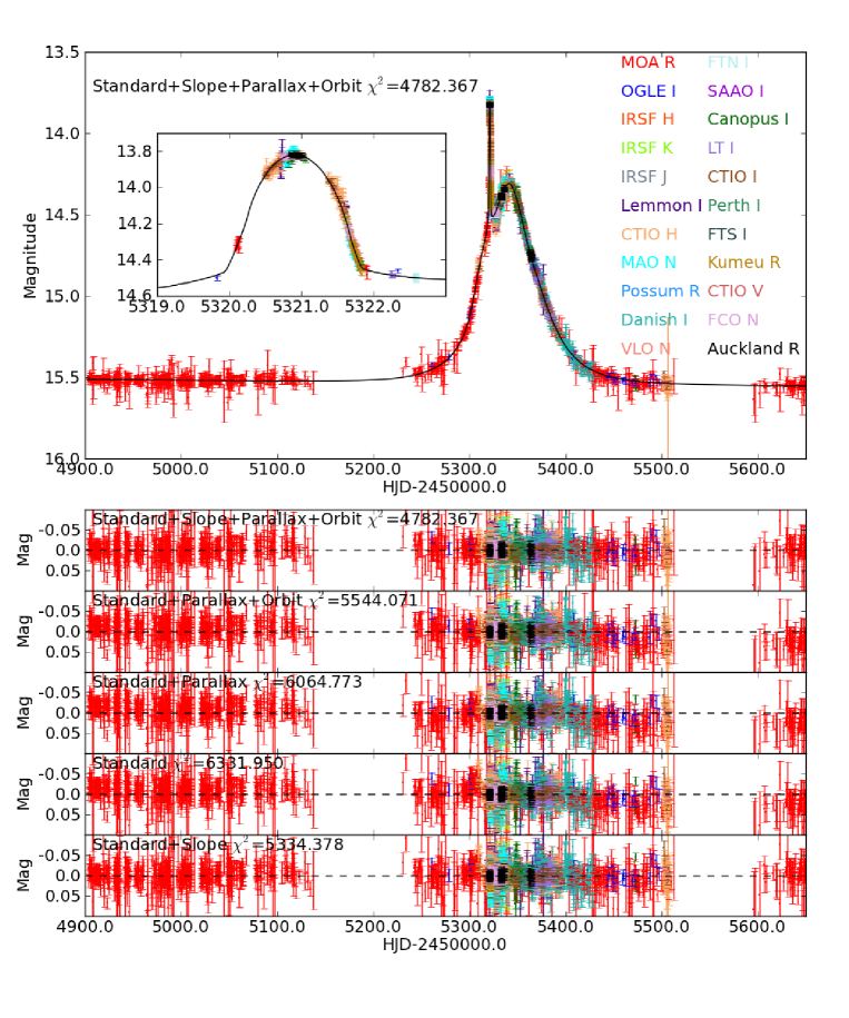
Figure 1: Top panel: The complete light curve of MOA-2010-BLG-073 with the data sets from the various observatories overlaid with our best fitting model. The inset shows the anomaly in greater detail. Lower panels: The residuals of the fit for each of the best-fitting models of each class.

3 Variability of the Source Star

MOA-2010-BLG-073 was present in the fields of the OGLE-II and OGLE-III surveys so the source star’s I-band photometric record extends from 1998 to 2006 (Fig. 2). OGLE-IV was in the commissioning phase when this event took place. From this excellent baseline it was immediately clear that the source is variable over many-month time scales. This raised the possibility that shorter-term variability might obfuscate the microlensing signal, making it difficult to determine its properties.

To investigate this possibility, we performed a search for periodicities in the baseline OGLE-II and OGLE-III data, excluding the lensing event, using the ANOVA algorithm (Schwarzenberg-Czerny, 1996). Due to the seasonal gaps in the baseline, we analyzed the OGLE-II data in yearly subsets as it is the best sampled, searching for periods between $P$=0.5–200 d. As Figure 3 demonstrates, there are no significant or persistent periodicities, other than the expected integer multiples of the 1-day sampling alias.

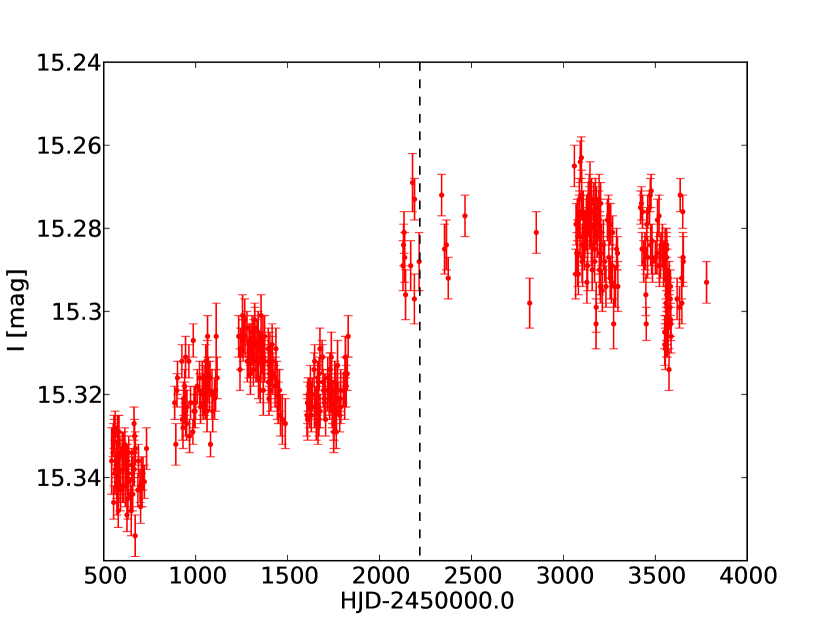
Figure 2: All available OGLE-II (1998–2001) and OGLE-III (June 2001–2006) lightcurve data for the source star of MOA-2010-BLG-073, taken prior to the event. The instrument upgrade to OGLE-III occurred around HJD=2452000.0. The apparent offset in magnitude at this time may be due in part to the difficulties of accurately calibrating photometry between the two wide field surveys.

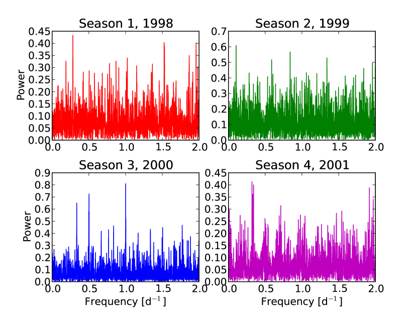
Figure 3: Periodograms of the OGLE-II (1998–2001) seasons of data, analyzed separately with the ANOVA algorithm. No significant periodicities were found in the range $P$=0.5–200 d, aside from the expected aliases.

We then combined the OGLE-II and III data sets in order to search for periods up to $P$=4000 d. Figure 2 indicates a slight ($\sim$0.04 mag) magnitude offset between the OGLE-II and III data. This can occur as a residual of OGLE’s photometric calibration between the two surveys but it might also be the result of the intrinsic stellar variation. Therefore, we performed a search for periods between 0.5 and 4000 d based on the combined data both with and without this offset (estimated visually). In both cases the periodogram was dominated by the window function; the only significant power was found in the peaks marking multiples of the 1-day alias, plus one peak at extreme low frequency corresponding to the finite length of the data set. We conclude that this star is an irregular, long-term variable, most likely as a result of pulsations.

However, there remained the possibility that the star could be irregularly variable on time scales comparable to that of the lensing event. To test this possibility, we binned the OGLE-II light curve on a range of time scales between 2–1200 d. To each bin we fitted two functions: one of constant brightness, and one with a linear slope and calculated the weighted root-mean-square (RMS) photometric scatter around each function per bin. We plot the average and maximum RMS (calculated over all bins in the lightcurve) against the width of the bins in time in Figure 4. On time scales shorter than 200 d the RMS scatter in the binned light curve is reasonably constant implying no significant short term variability. The longer term trend becomes clearly evident in the constant brightness curves for time scales longer than 400 d. We note that for bin widths between $\sim$800–1200 d, this curve has an RMS actually exceeding that of the whole light curve; this is because these bins were sufficiently wide that the first bin included the majority of the data, and the most variable sections of the light curve. As the bin widths became longer, they included more data points from the relatively stable section towards the end of the OGLE-II data set, and the RMS drops. The deviation of the OGLE lightcurve from a constant brightness exceeds 3$\sigma$ for timescales longer than $\sim$750 d. However, it deviates from a linear slope by $\leq$1.6$\sigma$ for timescales less than 1000 d, so we represent this variation as a gradient in the lightcurve over the duration of the event.

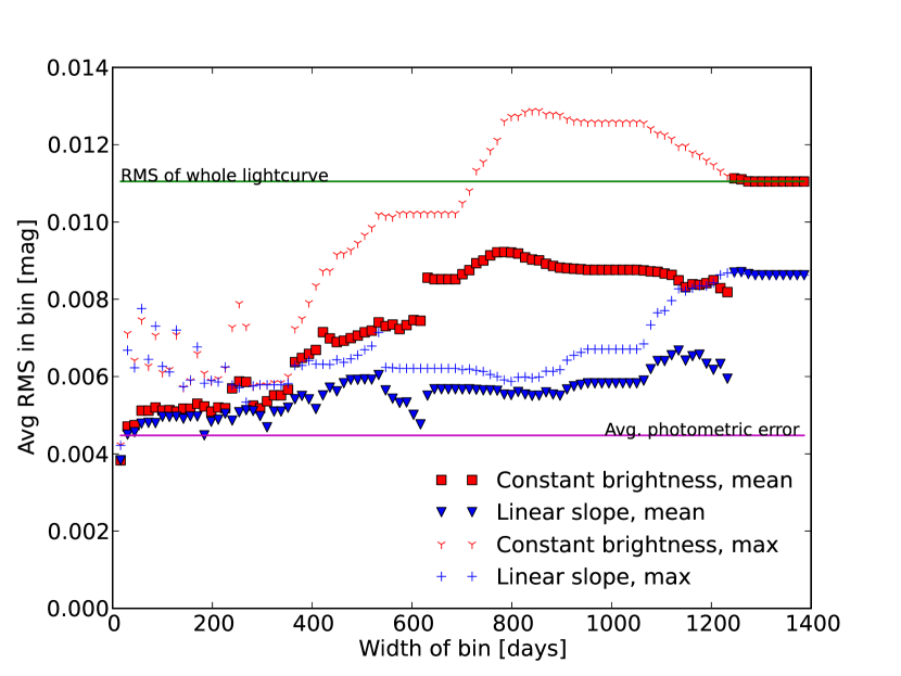
Figure 4: The OGLE-II photometry was binned using a series of bins of varying width in time. The data in each bin was fitted with two functions a) constant brightness b) with a linear slope, and the RMS around these curves was averaged over all the bins in the lightcurve. The average and maximum RMS for each binning is plotted here against the width of the bin, indicating variability over different timescales.

The most intuitive way to account for the variation of the source was to measure the gradient of the lightcurve taken at baseline immediately before and after the event. Unfortuantely only one of the available datasets covered these periods. Fitting a straight-line model (via a non-linear least-squares Marquardt-Levenberg algorithm) to the MOA 2009 and 2011 season data, we measured a slope of 0.018 mag/yr. However, the RMS scatter in the residuals of this fit were 0.016 mag, making it difficult to properly determine the slope. Additionally, in order to remove this slope from the other datasets, it would be necessary to transform the fluxes measured by each telescope on to the same scale as the MOA data. We attempted this via a linear regression approach but found that significant residuals remained. These contributed to overall higher $\chi^{2}$ values when the corrected data were fit with binary lensing models. We therefore adopted the alternative method of incorporating the slope as an additional parameter in our lensing model which we fit to the original, uncorrected data and we describe this approach in the following sections.

4 Analysis

In the analysis of this event, we used the established modeling software developed by S. Dong and C. Han (Dong et al., 2006; Shin et al., 2012b).

4.1 Initial Parameters

As a starting point for our analysis, we needed approximate values for the three parameters of the standard model for a PSPL event (not yet including the slope; this is discussed in § 4.8): $t_{\rm{0}}$, the time of peak magnification occurring at the closest projected separation between the lens and source, $u_{\rm{0}}$ and the Einstein radius crossing time, $t_{\rm{E}}$. Following standard convention, all distances are quoted in units of the angular Einstein radius, $\theta_{\rm{E}}$, of the lens.

To estimate these parameters, we combined all available data sets into a single light curve using the following scaling to take account of the varying degrees of PSF blending from different instruments:

$$f(t,k)=A(t)f_{s}(k)+f_{b}(k),$$ (1)

where $f(t,k)$ is the measured flux of the target at time $t$ from data set $k$, $A(t)$ is the lensing magnification at that time, $f_{s}$$(k)$ is the flux of the source star and $f_{b}$$(k)$ represents the flux of all stars blended with the source in the data set. A regression fit was used to measure $f_{s}$ and $f_{b}$ for each data set, producing an aligned light curve. Although the resulting parameter estimates are somewhat different from their ‘true’ values due to the existence of the anomalous deviation on the light curve, they provided a starting point in parameter space.

We note that two additional parameters can contribute to a PSPL model. They are the lens parallax parameters $\pi_{{\rm E},N}$ and $\pi_{{\rm E},E}$ that account for the light curve deviation caused by the motion of the Earth in its orbit over the course of the event. The vector microlens parallax, $\vec{\pi_{\rm{E}}}=AU/\widetilde{r_{\rm{E}}}$, where $\widetilde{r_{\rm{E}}}$ is the Einstein radius projected onto the observer plane and:

$$\vec{\pi}_{\rm E}\equiv(\pi_{{\rm E},N},\pi_{{\rm E},E})\equiv(\cos{\phi_{\pi}},\sin{\phi_{\pi}})\pi_{\rm{E}},$$ (2)

where $\phi_{\pi}$ represents the direction of lens motion relative to the source as a counter-clockwise angle, north through east. However, this is generally significant only for long ($\sim$months) time scale events, and was included at a later stage (see Section 4.6).

4.2 Finite Source

The sharp spike feature in the lightcurve is indicative of the source closely approaching or crossing a caustic. In these circumstances, it cannot be approximated by a point light source and must be treated as a disk of finite angular radius, $\rho$, with wavelength-dependent limb-darkening. This is addressed within our software using the ray-shooting approach (Kayser et al., 1986): the path of light rays is traced from the image plane back to the source, taking into account the bending of the trajectory according to the lens equation. If a ray is found to “land” within the radius of the source, its intensity is computed taking limb-darkening into account. We derived this from the linear limb darkening law:

$$I_{\lambda}(\cos{\phi})=I_{\lambda}(1)\left[1-u_{\lambda}(1-\cos{\phi})\right],$$ (3)

where $I_{\lambda}$ is the intensity of the source at radius $\phi$ from the center, relative to the central intensity $I_{\lambda}(1)$ in the same wavelength, $\lambda$, scaled by the coefficient $u_{\lambda}$. While more accurate limb darkening models are available, they are not commonly used in microlensing analyses due to the complexity introduced by combining data from many sources (Bachelet et al. (2012) discussed this in more detail). The values of $u_{\lambda}$ for each passband were calculated from the Kurucz ATLAS9 stellar atmosphere models presented by Kurucz (1979) using the method of Heyrovský (2007). However, within the microlensing community and software, Equation 3 more commonly follows the formalism derived by Albrow et al. (1999):

$$I_{\lambda}=\frac{F_{\lambda}}{\pi\theta_{*}^{2}}\left[1-\Gamma_{\lambda}\left(1-\frac{3}{2}\cos{\phi}\right)\right],$$ (4)

where $F_{\lambda}$ is the total flux from the source in a given passband and $\phi$ is the angle between the line of sight to the observer and the normal to the stellar surface. The limb darkening coefficient, $\Gamma_{\lambda}$ is related to $u_{\lambda}$ by:

$$\Gamma_{\lambda}=\frac{2u_{\lambda}}{3-u_{\lambda}}.$$ (5)

The values of $u_{\lambda}$ and $\Gamma_{\lambda}$ applied for each dataset are presented in Table 1. The lensing magnification is then computed as the ratio of the number of rays reaching the source plane relative to the number in the image plane. This approach is only required while the source is close to the caustic. At larger separations, the software employs a semi-analytic hexadecapole approximation to the finite source calculation to improve computation speeds (Pejcha & Heyrovský, 2009; Gould, 2008).

4.3 Standard Binary Model Grid Search

To model the light curve of a binary lens event, we introduced three additional parameters: $q=M_{L,2}/M_{L,1}$, the ratio of the masses of the two bodies composing the lens where $M_{L,1}$ is the more massive component, $s_{0}$, the projected separation of those masses and $\alpha_{0}$, the angle of the trajectory of the lensed source star, relative to the lens’ binary axis. The frame of reference was defined to be at rest with respect to the Earth at time $t_{0,\rm{par}}$, which we took to be the time of caustic crossing at HJD=2455321.0, estimated from the easily identifiable feature in the light curve (following the notation of Skowron et al. 2011).

With seven variables in the model ($t_{\rm{0}}$, $u_{\rm{0}}$, $t_{\rm{E}}$, $\alpha_{0}$, $s_{0}$, $q$, $\rho$), a number of different lens/source configurations may produce similar light curves, so it was necessary to thoroughly explore a large area of parameter space in order to ensure all possible solutions are identified. We therefore constructed a grid of models, spanning set ranges in the values of the three variables upon which the overall $\chi^{2}$ of the fit depended most sensitively, $s_{0}$, $q$ and $\alpha_{0}$. Each node in this grid took fixed values of ($s_{0}$,$q$,$\alpha_{0}$) and used a Markov Chain Monte Carlo (MCMC) approach (Dong et al., 2006) to find the best fitting model by optimizing the other parameters. To improve efficiency, a magnification map is generated by rayshooting for each point in the grid from which the model light curves used to compute the $\chi^{2}$ are drawn. The grid covered the following range: $\log(s_{0})=-0.6:0.6$ in steps of 0.012, $\log(q)=-4.0:1.0$ in steps of 0.05 and $\alpha=0.0:6.3$ in steps of 0.6.

Mapping out the $\chi^{2}$ for each node in this grid, we found a number of local minima. Visual inspection of these models overlaid on the light curve demonstrated that some more closely followed the data than others. Our first pass analysis included substantial baseline photometry before and after the event. This was not well fit by the models due to the variability of the source and hence the $\chi^{2}$ map gave a distorted view of regions in parameter space that best match the event. For this reason, we proceeded by repeating the grid search using just data taken during 2010. This produced two clear minima in $\chi^{2}$ of which one model stood out as by far the best match to the data. We then conducted a refined grid search over this restricted region of parameter space, taking smaller incremental steps.

4.4 Optimized Standard Binary Model

The refined grid search produced a reasonable model, fitting the majority of the data from all telescopes. This was used as a guide to identifying likely outlying data points, for which the quality of the reduction was then checked. A handful of data points were removed at this stage. However, this model included only fixed values for $s_{0}$, $q$ and $\alpha_{0}$. To properly determine the standard binary model for this event, our next step was to allow the seven parameters ($t_{\rm{0}}$, $u_{\rm{0}}$, $t_{\rm{E}}$, $\alpha_{0}$, $s_{0}$, $q$, $\rho$) to be optimized during the MCMC fitting process, which used the grid search results as its starting point. At this point we included the extended baseline data from MOA for seasons 2009 and 2011, as these fall within the period for which the source’s variability can be approximated with a straight line; we address this in Section 4.8.

4.5 Normalization of Photometric Errors

When fitting microlensing events, the reduced $\chi^{2}$ of the fit on a per data set basis, $\chi_{\rm{red}}^{2}$, typically produces a range of values both less than and exceeding the expected unity value. This can occur as different groups have slightly different ways of estimating photometric errors, but can lead to over- or under-emphasis being placed on particular data sets during the modeling process.

A common technique to address this issue is to arrive at a complete model for the event and then use this model to renormalize the original photometric errors of each data set, $e_{\rm{orig}}$, according to the expression:

$$e_{\rm{new}}=a_{0}\sqrt{e_{\rm{orig}}^{2}+a_{1}^{2}}.$$ (6)

We first conducted the sequence of models described in the following sections in order to find the best model for the event. We then set the coefficients $a_{0}$, $a_{1}$ such that the $\chi_{\rm{red}}^{2}$ relative to that model equaled unity; the adopted values are given in Table 1. We then repeated our MCMC fitting process, starting with the Standard binary model and systematically adding parameters in to determine the extent of improvement in the model $\chi^{2}$ in each case. We compare models in Tables 2 & 3, and we plot the residuals ($\rm{data}-\rm{model}$) in Figure 1. In the following sections, the $\chi^{2}$ values given are those post-renormalization.

4.6 Parallax

Given that the event’s $t_{\rm{E}}$$\sim$44 d$\sim$0.12 yr, it was necessary to include parallax in our model. Using the parameters of the Standard Binary Model as a starting point, we allowed our fitting process to optimize for $\pi_{{\rm E},E}$, $\pi_{{\rm E},N}$ also. We found that this significantly reduced the $\chi^{2}$ of the overall fit to 6064.773. By default, this procedure explored models with positive projected separations at closest approach of the lens and source, that is $u_{\rm{0}}>0$, which we define as the source’s trajectory passing the caustic at positive values of $\theta_{y}$ in the lens plane (see Figure 6). For the standard model case the symmetry with respect to the binary axis of the caustic means that the $u_{\rm{0}}<0$ solutions are identical. However once parallax was included, this was no longer the case, so we also explored $u_{\rm{0}}<0$ solutions (this degeneracy is further discussed in Park et al. (2004)). The parameters of the $u_{\rm{0}}>0$ model were taken as a starting point for the fit, except that the sign of $u_{\rm{0}}$ was reversed and the $\alpha_{0}$ value became $2\pi-\alpha_{0}$. We found the best fitting $u_{\rm{0}}<0$ model to be slightly less favored, with $\chi^{2}$=6099.487.

4.7 Lens Orbital Motion

The mass ratio and projected separation determined from this model put this event close to the boundary between close and intermediate/resonant caustic structure. In this regime, small changes in the projected separation of the lensing bodies due to their orbital motion can effectively change the shape of the caustic (see Fig. 6) while the event is underway, sometimes causing detectable deviations in the lightcurve. To explore this possibility, we included additional parameters in our model to describe the change in projected binary separation, $ds/dt$ and the rate of change of the angle of the projected binary axis, $d\alpha/dt$. Again we found that the $u_{\rm{0}}>0$ model gave the best fit, with $\chi^{2}$=5544.071, compared with 5690.003 when $u_{\rm{0}}<0$. This type of orbital motion is classified as “separational” in the schema put forward by Gaudi (2009); Penny et al. (2010), and is detected in this event as the source happens to cross the cusp of the caustic in the position where the caustic changes most rapidly.

4.8 Sloping Baseline

While taking these second-order effects into account significantly improved the fit to the data, the overall $\chi^{2}$ remained rather high. Visual inspection of the light curve still showed a gradient, especially in the 2010 baseline before, relative to after, the event. Based on our analysis in § 3, this trend is likely to be part of the longer-term variability of the source and not associated with the microlens. In order to determine the true lens/source characteristics though, this trend had to be taken into account.

The OGLE-II and III data demonstrate that the source variation over the $\sim$150 d time scale of the event can be approximated by a straight-line, rather than a higher-order function. We therefore introduced a ‘slope’ parameter to our model, representing the linear rate of change in magnitude during the event. This further improved the $\chi^{2}$, and the best-fitting model was once again the $u_{\rm{0}}>0$ solution with $\chi^{2}$=4782.367.

We note that there exist degeneracies between the slope parameter and those for parallax and orbital motion as they can be used to fit similar residuals in the lightcurve. To test for possible degeneracies, we also fit a standard model plus the slope parameter alone and found that $\chi^{2}$=5334.378. The value for the slope from this model, -0.0160$\pm$0.0004, was consistent with that derived from the model including parallax and orbital motion, -0.0153$\pm$0.0004.

4.9 Second Order Effects

With the slope parameter included we had accounted for all the physical effects which we expected to be present in the lightcurve. Having found that the residuals showed no further variation at a level detectable above the photometric noise, we did not attempt to include second order effects such as xallarap etc.

4.10 Final Model

All our models are compared in Table 2 and the parameters of the best-fitting models are presented in Table 3 and Figure 1. We plot the $\chi^{2}$ for each link in the MCMC chain for all parameters against one another in the best-fitting model in Figure 5. This plot was used as a diagnostic throughtout the fitting process, as any correlations between parameters display distinct trends as the chain moves towards the minimum. The caustic structure changed during the course of event, so in Figure 6 we show the structure at two distinct times; the first at the time of the first caustic crossing during the anomaly, and the second at the time of closest approach.

Table 2: The $\chi^{2}$for the best-fitting model in each class, comparing $u_{\rm{0}}>0$ and $u_{\rm{0}}<0$ solutions.

Model	$\chi^{2}$
	$u_{\rm{0}}>0$	$u_{\rm{0}}<0$
Standard	6331.950	6331.950
Standard+Parallax	6064.773	6099.487
Standard+Parallax+Orbital Motion	5544.071	5690.003
Standard+Parallax+Orbital Motion with Slope	4782.367	4802.606
Standard+Slope	5334.378	5334.378

Table 3: The best fitting parameters.

Parameter	Standard	Standard	Standard	Standard+Parallax	Standard+Parallax
(Units)		+Slope	+Parallax	+Orbital Motion	+Orbital Motion+Slope
$\chi^{2}$	6331.950	5334.378	6064.773	5544.071	4782.367
$\Delta\chi^{2}$b	1549.583	552.011	1282.406	761.704	0.0
$t_{\rm{0}}$ (HJD′)	5344.32	5344.38	5344.47	5344.83	5344.69
	$\pm$0.01	$\pm$0.01	$\pm$0.02	$\pm$0.03	$\pm$0.02
$u_{\rm{0}}$	0.4089	0.403	0.403	0.381	0.386
	$\pm$0.0009	$\pm$0.001	$\pm$0.001	$\pm$0.001	$\pm$0.001
$t_{\rm{E}}$ (d)	43.82	44.84	43.49	43.4	44.3
	$\pm$0.08	$\pm$0.09	$\pm$0.09	$\pm$0.1	$\pm$0.1
$s_{0}$	0.7692	0.7725	0.7717	0.7792	0.7750
	$\pm$0.0005	$\pm$0.0005	$\pm$0.0006	$\pm$0.0007	$\pm$0.0007
$q$	0.0705	0.0677	0.0695	0.0683	0.0654
	$\pm$0.0005	$\pm$0.0005	$\pm$0.0006	$\pm$0.0006	$\pm$0.0006
$\alpha_{0}$	0.180	0.171	0.198	0.297	0.221
	$\pm$0.003	$\pm$0.003	$\pm$0.003	$\pm$0.006	$\pm$ 0.007
$\rho$	0.01963	0.01912	0.01931	0.0163	0.0165
	$\pm$0.00006	$\pm$0.00007	$\pm$0.00008	$\pm$0.0001	$\pm$0.0001
$\pi_{{\rm E},N}$			0.18	0.96	0.37
			$\pm$0.02	$\pm$0.04	$\pm$0.05
$\pi_{{\rm E},E}$			-0.124	0.09	0.01
			$\pm$0.007	$\pm$0.01	$\pm$0.01
$ds/dt$ ($\rm{yr}^{-1}$)				0.53	0.49
				$\pm$0.02	$\pm$0.02
$d\alpha/dt$ ($\rm{yr}^{-1}$)				-1.21	-0.37
				$\pm$0.06	$\pm$0.08
Slope (mag/yr)		-0.0160			-0.0153
		$\pm$0.0004			$\pm$0.0004

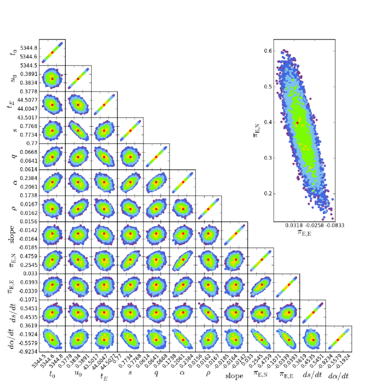
Figure 5: Chi squared contours plotted as a function of the parameters fitted in the MCMC fit for the best model. The red, orange, green, light blue, dark blue and purple colors indicate the regions with $\Delta\chi^{2}$$<$1–6$\sigma$ (respectively) from the best-fit solution. Inset: Close-up of the coutours for the parallax parameters.

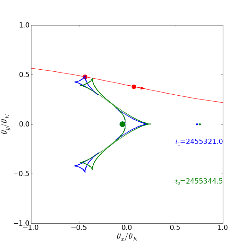
Figure 6: Maps of the caustic structure during the anomaly and at the time of closest approach. The red line and arrow indicate the trajectory of the source in a reference frame centered on the barycenter of the lensing system, while the red dots indicate the position of the source at these times. The green and blue dots indicate the positions of $M_{L,1}$ (largest) and $M_{L,2}$ at both times (radii of dots not to scale).

5 Physical Parameters

The purpose of this model is to ultimately arrive at the physical parameters of the lens and source, which can be achieved using the known relations between these and the lensing parameters obtained from the modeling.

Chiefly of interest is the mass of the lensing system, $M_{L,\rm{tot}}$, which can be determined explicitly for events where parallax is measurable provided the angular extent of the Einstein radius, $\theta_{\rm{E}}$, is known from:

$$M_{L,\rm{tot}}=\frac{c^{2}}{4G}\widetilde{r}_{\rm{E}}\theta_{\rm{E}}=\frac{c^{2}AU}{4G}\frac{\theta_{\rm{E}}}{\pi_{\rm{E}}},$$ (7)

where $\widetilde{r}_{\rm{E}}$ is the Einstein radius projected from the source onto the observer’s plane. The model parameter $\rho$ represents the angular size of the source star $\theta_{S}$ in units of the angular Einstein radius $\theta_{\rm{E}}$. We derive this from the crossing time taken for the source to travel behind the lens, $t_{*}=\mu\theta_{S}$ where $\mu$ is the relative source-lens proper motion. $\rho$ can then be written as:

$$\rho=\frac{t_{*}}{t_{\rm{E}}}=\frac{\theta_{S}}{\theta_{\rm{E}}},$$ (8)

These parameters also yield the distance to the lens,

$$\frac{AU}{D_{L}}\equiv\pi_{L}=\theta_{\rm{E}}\pi_{\rm{E}}+\frac{AU}{D_{S}}$$ (9)

which in turn yields the projected separation between the lens components:

$$a_{\perp}=s_{0}D_{L}\theta_{\rm{E}},$$ (10)

and the relative proper motion between lens and source, when combined with $t_{\rm{E}}$:

$$\mu=\frac{\theta_{\rm{E}}}{t_{\rm{E}}}.$$ (11)

The appreciable lens orbital motion during this event also allows us to test whether the companion object is bound to the primary lensing mass, via the ratio of its kinetic to potential energy:

$$\rm{KE}/\rm{PE}=\frac{(s_{0}R_{E})^{3}\gamma^{2}}{8\pi^{2}M_{L}},$$ (12)

where $\gamma$ relates the two lens orbital parameters: $\gamma^{2}$=($ds/dt$/$s_{0}$)² + ($d\alpha/dt$)² and where the masses are in units of $M_{\odot}$, the distances in AU and time measured in years.

However, these expressions include two key terms which are as yet, unknown: $\theta_{S}$, the angular source radius and $D_{S}$, the distance to the source. In order to extract the physical characteristics of the lens, we therefore turned our attention to the characteristics of the source.

5.1 Source Star

Long-exposure $V$, $I$ images were acquired by the CTIO 1.3 m at several epochs which enabled us to plot the color-magnitude diagram for the field including the source star (Fig. 7). By observing the event at different levels of lensing magnification, these data can be incorporated into the model which yields the source and blended light fluxes, $f_{s}$, $f_{b}$ for those data, and hence the instrumental magnitudes and colors of the source and blend. But we note that these uncalibrated fluxes also suffer from the high degree of extinction along the line of sight to the Galactic Bulge. To calculate the dereddened color, $(V-I)_{S,0}$, and magnitude, $I_{S,0}$, of the source, we needed to calibrate the instrumental fluxes $f_{s}$ and $f_{b}$ relative to a standard candle.

Fig. 7 clearly shows a locus of stars centered at $I_{\rm{RC},\rm{inst}}$=15.821$\pm$0.05 mag, $(V-I)_{\rm{RC},\rm{inst}}$=-0.350$\pm$0.05 mag. This consists of a clump of red giant stars, for which stellar theory predicts a stable absolute luminosity, varying only slightly with age and chemical composition. Their frequent occurrence makes these objects useful as standard candles. Stanek et al. (1998) established photometric calibrations for red clump magnitudes which were later refined by Alves et al. (2002) using Hipparcos data. Most recently, Nataf et al. (2012) were able to measure the dereddened apparent magnitude of the red clump stars at the Galactocentric distance, $I_{\rm{RC},\rm{0}}$= 14.443. By mapping the distances, $D_{RC}$, to red clump stars in the Galactic Bar as a function of Galactic longitude, $l$ they found an apparent viewing angle on the Bar of $\phi_{\rm Bar}$=40^∘,

$$\frac{R_{0}}{D_{RC}}=\frac{\sin{\phi+l}}{\phi}=\cos{l}+\sin{l}\cot{\phi},$$ (13)

where Nataf et al. (2012) measured $R_{0}$ to be 8.20 kpc. For the field of MOA-2010-BLG-073 (Galactic coordinates: $l$=4.81030^∘, $b$=-3.50131^∘), we derive $D_{RC}$=7.48 kpc, and we assumed that the source star lies behind the same amount of dust as the Red Clump stars and at the same distance. Scaling the dereddened apparent magnitude of the red clump stars, $I_{\rm{RC},\rm{0}}$, appropriately for the slightly closer distance of the stars in this field, $I_{RC,\rm{app}}$= $I_{\rm{RC},\rm{0}}$+ $\Delta I$, where:

$$\Delta I=5\log_{10}{R_{0}/D_{RC}}.$$ (14)

We found $\Delta I$ = 0.20 mag, and so the distance modulus to the red clump and the source in this field is $I_{RC,\rm{app}}$= 14.24 mag. Bensby et al. (2011) determined the intrinsic $(V-I)_{\rm{RC},\rm{0}}$=1.09 mag for red clump stars, so we were able to derive their absolute $V$ magnitude of $M_{V,RC,O}$=0.97 mag. Combining these results with the measured $\Delta(V-I)_{\rm inst}$ and $\Delta V_{\rm inst}$ between the source and red clump in the CTIO data, we then derived the dereddened color, $(V-I)_{S,0}$ and magnitude $I_{S,0}$ of the source, summarized in Table 4.

Bessell & Brett (1988) provided a relationship between $(V-I)$ and $(V-K)$ color indices, and Kervella et al. (2004) related $(V-K)$ to angular radius for giant and dwarf stars. Having thus determined $D_{S}$ and $\theta_{S}$, we derived the physical parameters of the lensing system, which are also summarized in Table 4. The color and large source radius of 14.7$\pm$1.3 $R_{\odot}$ implies this star is a K-type giant, which is consistent with the observed photometric variability. Jorissen et al. (1997) found that red giant stars with spectral types later than early-K are all variable, with amplitudes increasing from microvariability to several magnitudes towards cooler temperatures and timescales from days to years. Kiss et al. (2006) notes that irregular photometric variability may be caused by large convection cells, or may actually be the result of a number of simultaneous periodic pulsation modes, and many examples have been identified from time-domain surveys (Wray et al., 2004; Woźniak et al., 2004; Eyer & Blake, 2005; Ciechanowska et al., 2006, e.g.). We note that the star was detected by 2mass (Skrutskie et al., 2006) as source 2MASS J18101138-2631226 (catalog 2MASS~J18101138-2631226) with colors $(J-H)$=0.76$\pm$0.078 mag and $(H-K_{S})$=0.284$\pm$0.079 mag. Although the 2mass field is crowded the star’s PSF is distinct and their photometry for it has the best-quality AAA flag. These colors are consistent with a giant star and with our derived value for $K_{S,0}$=12.345 mag, when we take into account $AK_{S}$=0.24 mag from the vvv survey (Gonzalez et al., 2012).

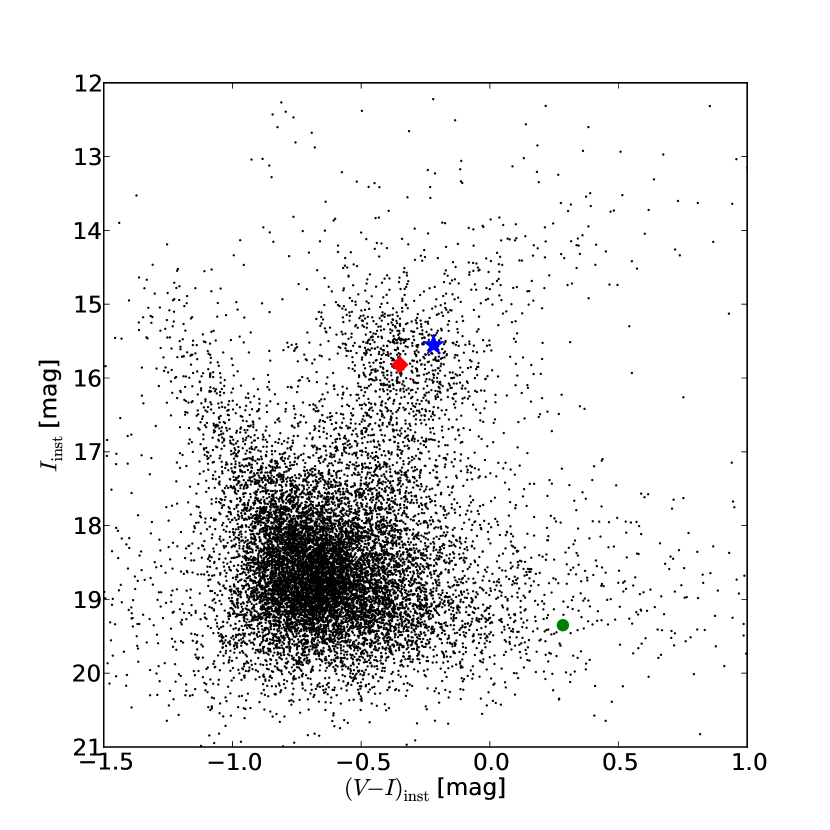
Figure 7: The instrumental color-magnitude diagram for the field of view including the lensing source star. The position of the source is marked with a blue star, relative to the center of the Red Giant Clump highlighted with a red diamond. The green circle indicates the color and $V$ magnitude of light blended in the CTIO photometry.

Table 4: The physical parameters of the lensing system and source star, derived from the model including slope, parallax and orbital motion, plus color information.

Parameter	Units	Value
$\theta_{S}$	$\mu$as	9.143$\pm$0.792
$\theta_{\rm{E}}$	mas	0.557$\pm$0.09
$R_{S}$	$R_{\odot}$	14.7$\pm$1.3
$M_{L,1}$	$M_{\odot}$	0.16$\pm$0.03
$M_{L,2}$	$M_{\rm{J}}$	11.0$\pm$2.0
$M_{L,\rm{tot}}$	$M_{\odot}$	0.17$\pm$0.03
$D_{L}$	kpc	2.8$\pm$0.4
$a_{\perp}$	AU	1.21$\pm$0.16
KE/PE		0.079
Proper motion	mas yr-1	4.60$\pm$0.4
$I_{S,\rm{inst}}$	mag	15.554$\pm$0.007
$V_{S,\rm{inst}}$	mag	15.335$\pm$0.007
$(V-I)_{S,\rm{inst}}$	mag	-0.22$\pm$0.01
$I_{\rm{RC},\rm{inst}}$	mag	15.821$\pm$0.05
$(V-I)_{\rm{RC},\rm{inst}}$	mag	-0.350$\pm$0.05
$I_{\rm{RC},\rm{0}}$	mag	14.443
$(V-I)_{\rm{RC},\rm{0}}$	mag	1.09
$I_{S,0}$	mag	13.976
$V_{S,0}$	mag	15.197
$(V-I)_{S,0}$	mag	1.221$\pm$0.051
$(V-K)_{S,0}$	mag	2.852
$K_{S,0}$	mag	12.345
$J$ (2mass)	mag	13.686$\pm$0.053
$H$ (2mass)	mag	12.926$\pm$0.057
$K_{S}$ (2mass)	mag	12.642$\pm$0.054

Nataf et al. (2012) explain that their value of our viewing angle of the Galactic Bar is a “soft upper bound” because the distance along the plane to the greatest density of stars along the line-of-sight to a triaxial Bar structure is less than the distance to the structure’s major axis on the far side and greater on the near side. As the physical parameters derived for MOA-2012-BLG-073 are somewhat dependent on the value of our viewing angle of the Galactic Bar and Nataf et al. (2012) quote consistent results with values as low as 25^∘, we explored the potential impact of this on our results. A reduced viewing angle would produce a smaller distance to the source, changing it’s dereddened magnitude and color. The resulting increase in source radius produces a corresponding reduction in the value of $D_{L}$and increases in the lens masses. However we found that the physical parameter values do not change by more than the errors quoted in Table 4, implying that this is not the dominant source of uncertainty. Finally, we computed the physical parameters derived from the best-fitting $u_{\rm{0}}<0$model for comparison and found that the masses derived changed by $<1\sigma$.

6 Discussion

The Earth’s movement during this relatively long time scale ($t_{\rm{E}}$=44.3 d) microlensing event resulted in a gradual shift in our perspective on the lensing system, breaking the symmetry of the caustic. Meanwhile, the change in projected separation of the lensing objects modified the shape of the caustic just as the source’s trajectory happened to pass close by. If not for these subtle variations, it can be seen from Figure 6 that a source trajectory $u_{\rm{0}}>0$ would produce exactly the same light curve as a $u_{\rm{0}}<0$ trajectory. As it is, for this event, the $u_{\rm{0}}>0$  solution best explains our observations, though the difference in $\chi^{2}$ relative to the corresponding $u_{\rm{0}}<0$ solution is very small ($\Delta\chi^{2}$=20.2) compared with the $\chi^{2}$ of both fits.

The measurable parallax signature enables us to determine the masses of the lensing bodies. The primary lensing object has $M_{L,1}$=0.16$\pm$0.03 $M_{\odot}$, making it an M-dwarf star. The companion’s mass is $M_{L,2}$=11.0$\pm$2.0 $M_{\rm{J}}$. This places it the brown dwarf desert, though we note that this traditionally refers to close-in companions, and since microlensing and direct imaging measure only the projected separation, we know only their minimum orbital semi-major radii. Regardless, it is clear that MOA-2010-BLG-073L b is close to the mass threshold for deuterium burning ($\sim$0.012 $M_{\odot}$=12.6 $M_{\rm{J}}$) quoted as the nominal boundary between planets and brown dwarfs established by the IAU (Chabrier et al., 2005). So what kind of object is it?

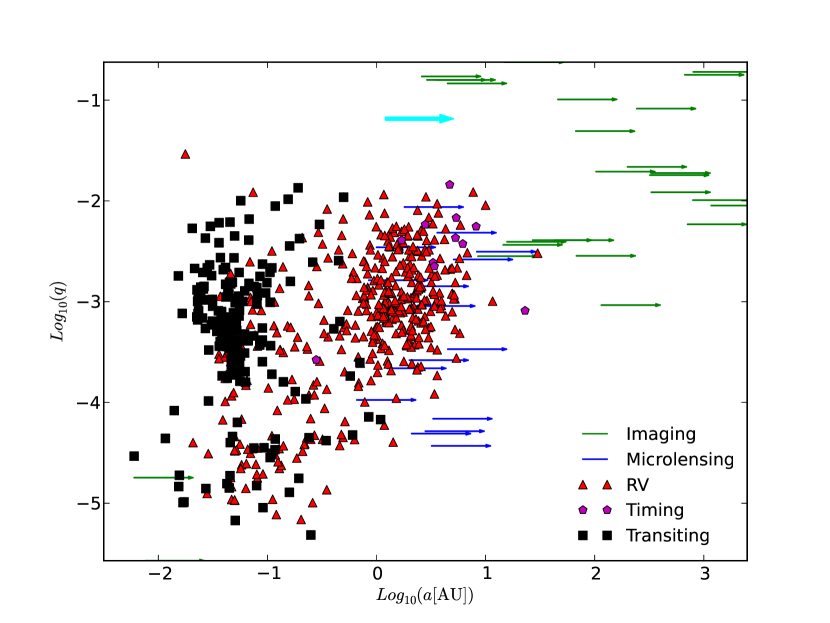
Figure 8: The ratio of planet mass to host star mass plotted against semi-major axis for all exoplanets for which these parameters are available (source: exoplanet.eu Schneider et al. (2011)). The true orbital semi-major axis is plotted where it has been measured, otherwise the projected (minimum) separation has been indicated with an arrow, where the base of the arrow marks the measured value. Very few objects have been found between $\log_{10}(q)$=-1 – -2. This corresponds to the brown dwarf desert. The location of MOA-2010-BLG-073L, highlighted in cyan and bold, lies between the brown dwarf and planetary regimes.

No further orbital or metallicity information is available for this event, which might have shed light on its evolutionary history. Theoretical isochrones predict that a star of this low mass will not have lost a significant amount of material over its lifetime, so we can say that MOA-2010-BLG-073L b formed as a high mass-ratio binary. Models of protoplanetary disks have the expectation that disk mass, $M_{D}$, will scale linearly with star mass $M_{*}$ (Williams & Cieza, 2011), $M_{D}/M_{*}\sim 1$% at young ages, but this would limit $M_{D}$ – and hence $M_{P,\rm{max}}$ – to $\sim$1–10 $M_{\rm{J}}$ in the case of MOA-2010-BLG-073L. So it seems questionable whether such a massive companion could have formed in a protostellar disk, via either core accretion or gravitational instability.

Bonnell et al. (2008); Kroupa & Bouvier (2003) discuss a number of mechanisms which can produce an M-dwarf/Brown Dwarf binary following gravitational fragmentation in a molecular cloud:

1. Embryo rejection model the nascent binary was ejected from a dynamically unstable multiple protostellar system, leading to the loss of its accretion envelope before the secondary component could acquire enough mass to become a star.

2. Collision model the binary was prematurely ejected from a larger protostellar system by the close passage of another star.

3. Photo-evaporation model the accretion envelope around the binary was photo-evaporated by the nearby presence of a massive star in the birth cluster before the secondary could accrete enough mass to become a star.

4. “Star-like” model the object formed as a normal stellar binary with low-mass components.

The embryo rejection model predicts (Bate, Bonnell & Bromm, 2002) that the maximum separation of binaries surviving this process is $a_{\rm{max}}\sim 10-20$ AU. We cannot rule out this scenario as we only measure the projected separation of the lens, which is nevertheless below $a_{\rm{max}}$. Since MOA-2010-BLG-073L is a field object we have no information regarding the proximity of other stars during its birth, so the collisional and photo-evapouration models are equally plausible. However, we note that Whitworth & Stamatellos (2006) derived a minimum mass for primary fragmentation components of 0.004 $M_{\odot}$$\sim$4.2 $M_{\rm{J}}$. As this threshold is below the mass of MOA-2010-BLG-073Lb the simplest explanation is that the companion is an extremely low-mass product of star formation. However, we note that the mass ratio of this system would match that of an object in the brown dwarf desert if the host were a more massive star. Recent surveys (Dieterich et al. (2012, e.g.); Evans et al. (2012, e.g.), though restricted to massive companions with $a>10$ AU) hint that the brown dwarf desert may extend to M-dwarfs and beyond 3 AU, which would make MOA-2010-BLG-073L a rare example of its type.

References

- Albrow et al. (1999) Albrow, M.D., Beaulieu, J.-P., Caldwell, J.A.R. et al. 1999, ApJ, 522, 1022.
- Albrow et al. (2009) Albrow, M. D., Horne, K., Bramich, D. M. et al. 2009, MNRAS, 397, 2099
- Alves et al. (2002) Alves, D. R., Rejkuba, M., Minniti, D.,Cook, K. H. 2002, ApJ, 573, L51
- Bachelet et al. (2012) Bachelet, E., Shin, I.-G., Han.C et al. 2012, ApJ, 754, 73.
- Beaulieu et al. (2006) Beaulieu, J.-P., Bennett, D.P.,Fouqué, P. et al. 2006, Nature, 439, 437.
- Baraffe et al. (2010) Baraffe, I., Chabrier, G.,Barman,T. 2010, Rep. Prog. Phys. 73, 016901.
- Bate, Bonnell & Bromm (2002) Bate, M.R., Bonnell, I.A., Bromm, V. 2002, MNRAS, 332, L65.
- Batista et al. (2011) Batista, V., Gould, A., Dieters, S. etal. 2011, A&A, 529, 102.
- Béjar et al. (2012) Béjar, V.J.S., Zapatero Osorio,M.R., Rebolo, R. et al. 2012, ApJ, 743, 64.
- Bensby et al. (2011) Bensby, T., Adén, D., Meléndez, J. et al. 2011, A&A, 533, 134.
- Bessell & Brett (1988) Bessell, M.S. & Brett, J.M.1988, PASP, 100, 1134.
- Bond et al. (2001) Bond, I., Abe, F., Dodd, R. J. et al. 2001, MNRAS, 327, 868.
- Bonnell et al. (2008) Bonnell, I.A., Clark, P., Bate, M.R.2008, MNRAS, 389, 1556.
- Bonfils et al. (2011) Bonfils, X., Delfosse, X., Udry, S. et al.2011, A&A, submitted.
- Boss (2006) Boss, A.P. 2006, ApJ, 643, 501.
- Bramich (2008) Bramich, D.M. 2008, MNRAS, 386, L77.
- Burrows et al. (2001) Burrows, A., Hubbard, J.I.,Lunine, J.I. et al. 2001, Rev. Mod. Phys., 73, 719.
- Chabrier et al. (2005) Chabrier, G., Baraffe, I., Allard,F. et al. 2005, ASP Conf. Series ”Resolved Stellar Populations”, Cancun.
- Chabrier et al. (2011) Chabrier, G., Leconte, J.,Baraffe, I. 2011, Proc. IAU Symp., 276, 171.
- Ciechanowska et al. (2006) Ciechanowska, A. et al. 2006, Acta Astron., 56, 219.
- Cumming et al. (2008) Cumming, A., Butler, R.P., Marcy, G.W. et al. 2008, PASP, 120, 531.
- Díaz et al. (2012) Díaz, R.F., Santerne, A., Sahlmann, J. et al. 2012, A&A, 538, A113.
- Dieterich et al. (2012) Dieterich, S.B., Henry, T.J., Golimowski, D.A. et al. 2012, AJ, 144, 64.
- Dominik et al. (2010) Dominik, M., Jørgensen, U.G., Rattenbury, N.J. et al. 2010, Ast. Nac., 331, 671.
- Dong et al. (2006) Dong, S., DePoy, D. L., Gaudi, B. S. et al. 2006, ApJ, 642, 842.
- Dong et al. (2009) Dong, S., Gould, A., Udalski, A. et al. 2009, ApJ, 695, 970.
- Evans et al. (2012) Evans, T.M., Ireland, M.J., Kraus, A.L. et al. 2012, ApJ, 744, 120.
- Eyer & Blake (2005) Eyer, L. & Blake, C. 2005, MNRAS, 358, 30.
- Fischer & Valenti (2005) Fischer, D.A. & Valenti, J. 2005, ApJ, 622, 1102.
- Forveille et al. (2011) Forveille, T., Bonfils, X., Lo Curto, G. et al. 2011, A&A, 526, A141.
- Gaudi (2009) Gaudi, B.S. 2009, Oral presentation at 13th Microlensing Workshop, Paris.
- Gonzalez et al. (2012) Gonzalez, O.A., Rejkuba, M., Zoccali, M. 2012, A&A, 543, A13.
- Gould et al. (2006) Gould, A., Udalski, A., An, D. et al. 2006, ApJ, 644, L37.
- Gould (2008) Gould, A. 2008, ApJ, 681, 1598.
- Heyrovský (2007) Heyrovský, D. 2007, ApJ, 656, 483.
- Howard et al (2012) Howard, A.W., Marcy, G.W., Bryson, S.T. et al. 2012, ApJ, 201, 15.
- Ida & Lin (2004) Ida, S. & Lin, D.N.C. 2004, ApJ, 616, 567.
- Ida & Lin (2005) Ida, S. & Lin, D.N.C. 2005, ApJ, 626, 1045.
- Johnson et al. (2007) Johnson, J.A., Butler, R.P., Marcy, G.W. et al. 2007, ApJ, 670, 833.
- Johnson et al. (2010) Johnson, J.A., Aller, K.M., Howard, A.W. et al. 2010, PASP, 122, 905.
- Jorissen et al. (1997) Jorissen, A., Mowlavi, N., Sterken, C., Manifroid, J. 1997, A&A, 324, 578.
- Kervella et al. (2004) Kervella, P., Bersier, D., Mourard, D. et al. 2004, A&A, 428, 587.
- Kayser et al. (1986) Kayser, R., Refsdal, S. & Stabell, R.1986, A&A, 166, 36.
- Kirkpatrick et al. (2006) Kirkpatrick, J. D., Barman, T. S., Burgasser, A. et al. 2006, ApJ, 639, 1120.
- Kiss et al. (2006) Kiss, L.L., Szabó, Gy.M., Bedding, T.R. 2006, MNRAS, 372, 1721.
- Klein et al. (2003) Klein, R., Apai, D., Pascucci, I. et al. 2003, ApJ, 593, L57.
- Kroupa & Bouvier (2003) Kroupa, P. & Bouvier, J. 2003,MNRAS, 346, 369.
- Kurucz (1979) Kurucz, R.L. 1979, ApJS, 40, 1.
- Laughlin et al. (2004) Laughlin, G., Bodenheimer, P. & Adams,F.C. 2004, ApJ, 612, L73.
- Luhman (2012) Luhman, K.L. 2012, ARA&A, 50, 65.
- Marcy & Butler (2000) Marcy, G.W. & Butler, R.P. 2000, PASP, 112, 137.
- Maldonado et al. (2012) Maldonado, J., Eiroa, C., Villaver, E. et al. 2012, A&A, 541, 40.
- Marois et al. (2008) Marois, C., MacIntosh, B., Barman, T., 2008, Science, 322, 1348
- Mordasini et al. (2009) Mordasini, C., Alibert, Y., Benz, W. 2009,A&A, 501, 1139.
- Miyake et al. (2012) Miyake, N., Udalski, A., Sumi, T. et al. 2012, ApJ, 752, 82.
- Nataf et al. (2012) Nataf, D.M., Gould, A., Fouqué, P. et al. 2012, ApJ,submitted.
- Park et al. (2004) Park, B.-G., DePoy, D.L., Gaudi, B.S. et al. 2004, ApJ, 609, 166.
- Pejcha & Heyrovský (2009) Pejcha, O. & Heyrovský, D. 2009, ApJ, 690, 1772.
- Penny et al. (2010) Penny, M.T., Mao, S. & Kerins, E. 2010, MNRAS, 412, 607.
- Santos, Israelian & Mayor (2001) Santos, N.C., Israelian, G. & Mayor, M. 2001, A&A, 373, 1019.
- Sahlmann et al. (2010) Sahlmann, J., Ségransan, D., Queloz, D. et al. 2010, A&A, 525, A95.
- Schneider et al. (2011) Schneider, J., Dedieu, C., Le Sidaner, P. et al. 2011, A&A, 532, A79.
- Scholz et al. (2006) Scholz, A., Jayawardhana, R. & Wood, K. 2006, ApJ, 645, 1498.
- Schwarzenberg-Czerny (1996) Schwarzenberg-Czerny, A. 1996,ApJ, 460, L107–L110.
- Shin et al. (2012a) Shin, I.-G., Han, C., Gould, A. et al. 2012, ApJ, in prep.
- Shin et al. (2012b) Shin, I.-G., Han, C., Choi, J.-Y. et al. 2012, ApJ, 746, 127.
- Skowron et al. (2011) Skowron, J., Udalski, A., Gould, A. et al. 2011, ApJ, 738, 87.
- Skrutskie et al. (2006) Skrutskie, M.F., Cutri, R.M., Stiening, R. et al. 2006, AJ, 131, 1163.
- Stanek et al. (1998) Stanek, K.Z. & Garnavich, P.M. 1998, ApJ, 503, 131.
- Sumi et al. (2003) Sumi, T., Bond, I. A., Dodd, R. J. 2003, ApJ, 591, 204.
- Sumi et al. (2011) Sumi, T., Kamiya, K., Bennett, D.P. et al. 2011,Nature, 473, 349.
- Tsapras et al. (2009) Tsapras, Y, Street, R., Horne, K. et al. 2009, Ast. Nac., 330,4.
- Udalski et al. (2003) Udalski, A. 2003, Acta Astron.,53, 291.
- Whitworth & Stamatellos (2006) Whitworth, A.P. & Stamatellos, D. 2006, A&A, 458, 817.
- Williams & Cieza (2011) Williams, J.P. & Cieza, L.A. 2011, ARA&A, 49, 67.
- Woźniak et al. (2004) Woźniak, P.R., Williams, S.J., Vestrand, W.T., Gupta, V. 2004, AJ, 128, 2965.
- Wray et al. (2004) Wray, J.J., Eyer, L., Paczyński, B. 2004,MNRAS, 349, 1059.
- Yee et al. (2012) Yee, J. C., Shvartzvald, Y., Gal-Yam, A. et al. 2012, ApJ, 755, 102.
- Zhou et al. (2012) Zhou, J.-L., Xie, J-W, Liu, H-G et al. 2012, Res. in Astron. & Astrophy., 12, 1081.