Asymmetry in the outburst of SN 1987A detected using light echo spectroscopy

Abstract

We report direct evidence for asymmetry in the early phases of SN 1987A via optical spectroscopy of five fields of its light echo system. The light echoes allow the first few hundred days of the explosion to be reobserved, with different position angles providing different viewing angles to the supernova. Light echo spectroscopy therefore allows a direct spectroscopic comparison of light originating from different regions of the photosphere during the early phases of SN 1987A. Gemini multi-object spectroscopy of the light echo fields shows fine-structure in the H$\alpha$ line as a smooth function of position angle on the near-circular light echo rings. H$\alpha$ profiles originating from the northern hemisphere of SN 1987A show an excess in redshifted emission and a blue knee, while southern hemisphere profiles show an excess of blueshifted H$\alpha$ emission and a red knee. This fine-structure is reminiscent of the “Bochum event” originally observed for SN 1987A, but in an exaggerated form. Maximum deviation from symmetry in the H$\alpha$ line is observed at position angles $16^{\circ}$ and $186^{\circ}$, consistent with the major-axis of the expanding elongated ejecta. The asymmetry signature observed in the H$\alpha$ line smoothly diminishes as a function of viewing angle away from the poles of the elongated ejecta. We propose an asymmetric two-sided distribution of ⁵⁶Ni most dominant in the southern far quadrant of SN 1987A as the most probable explanation of the observed light echo spectra. This is evidence that the asymmetry of high-velocity ⁵⁶Ni in the first few hundred days after explosion is correlated to the geometry of the ejecta some 25 years later.

1. Introduction

A light echo (LE) occurs when outburst light from an event is scattered by circumstellar or interstellar dust into the line of sight of the observer. LE imaging has long been used as a powerful tool for studying the three-dimensional dust structure surrounding supernovae (SNe) (Crotts, 1988; Xu et al., 1995; Sugerman et al., 2005; Kim et al., 2008). In 1988, spectra of the inner and outer LE rings of SN 1987A confirmed the resemblance to a maximum-light spectrum (Gouiffes et al., 1988; Suntzeff et al., 1988b). More recently, however, this technique of targeted LE spectroscopy has been used on historical SNe to identify the spectral type of the original outburst. After the serendipitous discovery of LEs from ancient SNe in the Large Magellanic Cloud (LMC) during the SuperMACHO project by Rest et al. (2005a), follow-up spectroscopy by Rest et al. (2008b) identified the type of SN responsible for the remnant SNR 0509-675. The spectral types of the Cas A and Tycho SNe have also been identified using this method of targeted LE spectroscopy (Rest et al., 2008a; Krause et al., 2008a, b). Rest et al. (2011b) used LE spectroscopy to detect asymmetries in the outburst of the Cas A SN, while Rest et al. (2012b) recently obtained LE spectroscopy from the “Great Eruption” of $\eta$ Carinae. We refer the reader to Rest et al. (2012a) for a review of LE spectroscopy emphasizing these more recent results. Given the acceleration of the field of LE spectroscopy in recent years, a detailed study of spectra of the well-known LE system of SN 1987A can provide a foundation for future studies, as well as provide new insight into the explosion of SN 1987A.

In the case of historical LEs, one has to use the photometric and spectroscopic history of a different SN to model the LE spectrum (see, e.g. Rest et al., 2011b, where the Cas A outburst is modeled with the lightcurve and spectra of SN 1993J and SN 2003bg). For SN 1987A, however, the exact spectral and photometric history of the LE source is known with high-precision, allowing observed LE spectra to be compared unambiguously to an isotropic scenario. In addition to acting as a test bed for LE spectroscopy theories, the near-circular LE rings of SN 1987A allow the original outburst to be probed for asymmetries in an entirely direct way. Different position angles (PAs) on the LE system probe different viewing angles from which we can view the time-integrated spectrum of the original event.

Observations as well as theoretical simulations indicate that core-collapse SNe are asymmetric in nature. Polarization measurements show deviations from spherical symmetry in all core-collapse SN with sufficient data (Wang & Wheeler, 2008), while recent simulations in two and three spatial dimensions show large deviations from symmetry (e.g., Hammer et al., 2010; Gawryszczak et al., 2010; Müller et al., 2012). Coupled with the fact that state of the art spherically symmetric core-collapse simulations in one spatial dimension fail at producing an explosion for $>10$M_☉ projenitors (Burrows, 2012), multi-dimensional physics such as the standing accretion shock instability (SASI; Blondin et al., 2003) may play a key role in understanding the explosion mechanism. As a new method for observing asymmetries, LE spectroscopy of SNe may be able to provide new insight into the origin of SN asymmetries and their relation to the core-collapse explosion mechanism.

SN 1987A was a peculiar Type II SN with a blue supergiant progenitor located in the LMC (see, e.g., Arnett et al., 1989, and references therein for a review of SN 1987A and its progenitor). SN 1987A was known to be an asymmetric SN. Early polarization measurements (e.g., Jeffery, 1987; Bailey, 1988; Cropper et al., 1988) and an elongated initial speckle image (Papaliolios et al., 1989) suggested a non-spherical event. Fine structure in the H$\alpha$ line (the “Bochum event”) at 20-100 days after the explosion as well as redshifted emission lines at more than 150 days after explosion provide strong evidence for radial-mixing of heavy elements into the upper envelope (Hanuschik & Dachs, 1987; Phillips & Heathcote, 1989; Spyromilio et al., 1990). Updated models of the bolometric lightcurve at early epochs also require radial-mixing of ⁵⁶Ni (Shigeyama & Nomoto, 1990; Utrobin, 2004). Direct HST imaging by Wang et al. (2002) showed an elongated remnant ejecta, claimed to be bipolar and showing evidence for a jet-induced explosion. Recent integral field spectroscopy of the ejecta by Kjær et al. (2010) showed a prolate structure for the ejecta oriented in the plane of the equatorial ring, arguing against a jet-induced explosion.

Here we present detailed imaging and spectroscopy of the SN 1987A LE system. We infer the relative contributions of the different epochs of the SN to the observed LE spectrum by modeling images of the LE, as demonstrated by Rest et al. (2011a). We fit the observed LE spectra and use specific examples to illustrate the models ability to correctly interpret the observations. We then use the LE spectra to probe for asymmetries in the explosion of SN 1987A and compare to previous observations of asymmetry.

2. Observations and Reductions

2.1. Imaging

Imaging of the SN 1987A LE system was performed under the SuperMACHO Project microlensing survey (Rest et al., 2005b) using the CTIO 4m Blanco telescope. The survey monitored the central portion of the LMC for five seasons beginning in 2001 using the 8K $\times$ 8K MOSAIC imager (plus atmospheric dispersion corrector) with the custom “VR” filter ($\lambda_{c}=625$ nm, $\delta\lambda=220$ nm). Exposure times were between 150 and 200 s. We have continued to monitor the field containing SN 1987A and its LEs (field sm77) since the survey ended. Data reduction and difference images were performed using the ESSENCE/SuperMACHO pipeline photpipe (Rest et al., 2005b; Garg et al., 2007; Miknaitis et al., 2007). A stacked and mosaiced difference image of the LE system is shown in Figure 1. The near-circular rings illuminate three general dust structures: a smaller structure $\sim 85$ pc in front of SN 1987A, only visible in the south; a near-complete ring at $\sim 185$ pc and brightest in the north-east; as well as a larger and fainter near-circular illumination at $\sim 400$ pc in front of the SNR. All three of these structures have been mapped previously in detail by Xu et al. (1995) and can be referred to as three “sheets” of ISM dust roughly in the plane of the sky. However, it is important to note that the LE flux observed in Figure 1 is due to dense filamentary structure within the general “sheets” of ISM dust. The physical properties of the scattering dust filaments (inclination and thickness) can vary greatly within what appears to be a uniform “sheet” of dust. This distinction is important to make when modeling the LE photometry and spectroscopy.

2.2. Gemini Spectroscopy

We obtained multi-object optical spectroscopy (MOS) for five fields of the SN 1987A echo system in the 2006B term, using the R400 grating and GG455 blocking filter on the Gemini Multi-Object Spectrograph (GMOS) on Gemini-South. SuperMACHO or GMOS preimages were differenced with previous SuperMACHO images to establish the precise location of the echo system, allowing the design of GMOS masks. The locations of five MOS fields and the 14 1.0^′′ wide LE slitlets are shown in Figure 1.

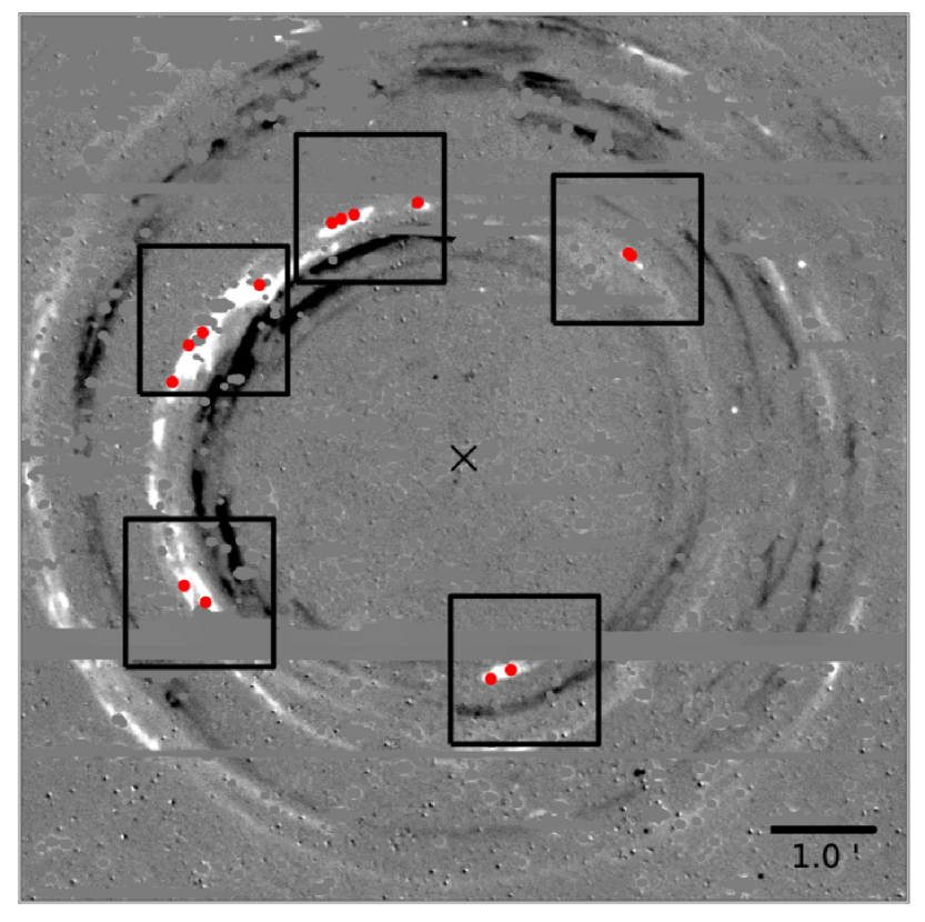
Figure 1.— Mosaiced SuperMACHO difference image of August 2006 and January 2002 epochs of the SN 1987A LE system. The locations of the 14 GMOS slits appear in red, while the black cross indicates the location of SNR. Slitlets are not to scale. The black squares collect LEs which were observed in the same MOS field. North is up and east is to the left.

The nod and shuffle mode of GMOS was used to best isolate the diffuse LE signal from the nebular sky background. To ensure clear sky in the offset position, the telescope was nodded off-source several degrees every 225 s. On-source integration times for the brightest echo fields were 30 minutes, and 90 minutes for the fainter, more diffuse echoes. During each night of observations, flat field and CuAr spectral calibration images were taken before or after the science images. We also acquired dark images with the same nod and shuffle parameters used during integration. These specialized dark images allow features associated with charge-traps in the GMOS CCDs to be masked out during reduction.

The observations result in LE spectra from SN 1987A with a spectral range of 4500-8500 Å, contaminated by strong emission lines from the nebular region, as well as any stellar continuum entering the slitlets. The P Cygni H$\alpha$ line seen in the spectra is further degraded due to six strong nebular emission lines ([NII] $\lambda$6548, H$\alpha$ $\lambda$6563, [NII] $\lambda$6585, HeI $\lambda$6678, [SiII] $\lambda$6717, [SiII] $\lambda$6731). Signal from the emission peak of the P Cygni H$\alpha$ line is therefore lost to nebular emission, and this region of the profile cannot be interpreted with confidence. In particular, the location and flux of the emission peak cannot be determined without interpolations which we found introduced large uncertainties.

The nebular contamination can be greatly reduced since the LE system is expanding superluminally on the sky (as seen in Figure 1). We therefore have the unique opportunity in astronomy to observe only the background sky signal at the same location on the sky as the initial sky+object observation. Sky-only observations were taken in the 2009A and 2009B semesters for the five MOS fields. The spectroscopy was carried out using the same GMOS configuration as the previous sky+object 2006B observations, with 30 minutes on-source integration times in nod and shuffle mode. The spectrophotometric standard star LTT 3864 was observed during the 2009A observations.

2.3. Spectra Reduction

All spectra were reduced using IRAF and the Gemini IRAF package, with bias subtraction and trimming done on each CCD individually. Science images were dark subtracted using the special nod and shuffle darks, with each CCD being cleaned of cosmic rays using the Laplacian rejection algorithm LACOSMIC (van Dokkum, 2001). Nod and shuffle sky subtraction was performed on each science exposure using the gnsskysub task. Individual slitlets were automatically cut from the wavelength calibrations frames, however this procedure required manual tweaking to achieve the best cutting possible. A wavelength solution was found for each slitlet in the calibration frame. Science frames were flattened, CCDs mosaiced together, and slitlets cut from the images. The wavelength solution for each slitlet was then applied to the corresponding science spectrum in two dimensions. Since the LE signal is so weak, determining an extraction aperture is very difficult. Instead, we collapsed the entirety of each slitlet to one dimension using a block average.

No suitable spectrophotometric standard star was observed during the 2006B observing semester, nor did a suitable standard star matching our unique instrument configuration exist in the data archive nearby temporally. However, the spectrophotometric standard LTT 3864 was observed during the 2009A observations. We therefore used the 2009A standard to perform the flux calibration for all of the 2006 and 2009 spectra. While this leads to large errors in absolute flux calibration, our analysis is independent of absolute flux levels. Instead, the purpose of the flux calibration used here is to remove the effect of CCD sensitivity from the spectra, which is relatively stable in time. A LE spectrum is a weighted average of many epochs from the outburst. Determining the continuum of such a spectrum is therefore difficult, and the alternative analysis procedure of removing the continuum from all of our spectra would have had a larger error than that of the flux calibration.

The sky-only spectra from 2009 were subtracted in one dimension from the 2006 LE spectra for each MOS slit. This procedure was performed interactively, adjusting the scale and wavelength of the sky spectrum in small increments using the IRAF task skytweak to minimize sky subtraction residuals in the final spectra. Since we focus our science analysis on the H$\alpha$ line, we performed the sky subtraction such that the subtraction residuals in the P Cygni profile of H$\alpha$ were minimized. All spectra were Doppler-corrected, adopting a LMC radial velocity of 286.5 km s^-1 (Meaburn et al., 1995).

3. Analysis

3.1. Light Echo Spectra

The upper panel of Figure 2 shows a reduced LE spectrum from the 2006 observations along with the underlying sky-only nebular spectrum from 2009. The high-velocity P Cygni profiles including H$\alpha$ resemble a Type II SN spectrum at maximum light, confirming the LE spectra probe the original outburst light of SN 1987A. Strong, narrow nebular lines not associated with the SN outburst dominate the spectrum around 5000Å and the H$\alpha$ line at 6563Å.

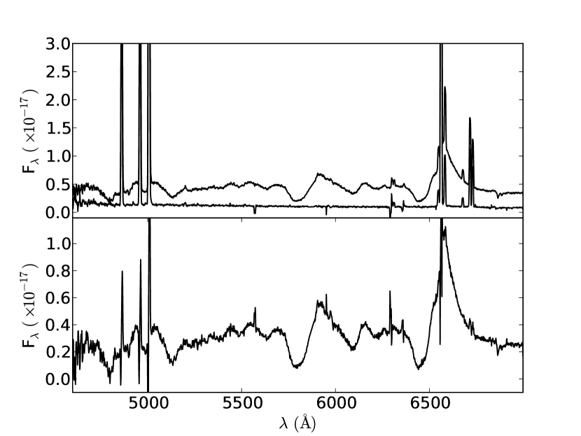
Figure 2.— Upper Panel: Example LE+sky spectrum from 2006 shown with the corresponding sky-only nebular spectrum from 2009. Lower Panel: The result of difference spectroscopy, showing the LE-only spectrum along with remaining nebular residuals from the subtraction. The strength of the H$\alpha$ emission peak can now be estimated in the difference spectrum.

The result of performing difference spectroscopy is shown in the lower panel of Figure 2, where the sky-only signal has been subtracted from the 2006 echo spectrum. Flux from the emission component of the H$\alpha$ line is recovered that was initially lost to nebular contamination. In the majority of our spectra we are able to resolve the H$\alpha$ emission peak without loss due to the nebular lines.

3.2. Modeled Isotropic Spectrum

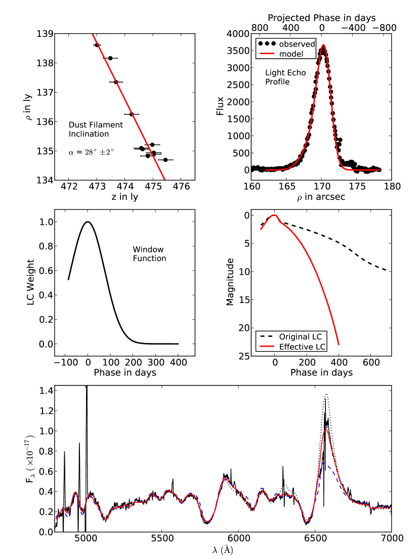
Figure 3.— Summary of modeling procedure for each LE spectrum. The inclination of the dust filament is measured (upper left panel), allowing the shape of the LE profile to be modeled to determine the dust width (upper right panel). The properties of the slit determine the window function containing the relative contribution from each epoch (middle left panel), which when multiplied by the original lightcurve gives the effective lightcurve for this observation (middle right panel). We integrate the historical spectra of SN 1987A, flux-weighted with the effective lightcurve, and take into account wavelength-dependent scattering and reddening to obtain a fit between the LE model and the observed spectrum (lower panel). The lower panel plot shows the model LE fit (solid red) along with the attempted fit with the maximum light spectrum of SN 1987A (dashed blue) and the full lightcurve-integrated spectrum (dotted black).

To search for asymmetries in SN 1987A using spectroscopy of its LEs, we need to first consider what defines asymmetry in observed spectra. As shown in Rest et al. (2011a), multiple LE spectra from the same transient source, with differing line strength ratios, does not necessarily imply an asymmetry in the outburst light. An observed LE spectrum will depend strongly on the physical properties of the scattering dust as well as the instrument configuration and seeing conditions at time of observation. Specifically, the dominant epochs of the original outburst probed by a LE spectrum can change with the above properties. Relative comparisons of LE spectra can therefore easily lead to false-detections of asymmetry if the above factors are not taken into consideration. Each LE spectrum should instead be compared to a single isotropic spectrum modeled for each observation. We define our isotropic model spectrum as the original outburst of SN 1987A, as it would have been spectroscopically observed if scattered by dust corresponding to the observed LE. This provides a direct probe of asymmetry since differences between observed and model spectra represent deviations from the historically observed outburst of SN 1987A.

A LE observed on the sky has a flux profile (flux versus $\rho$, where $\rho$ is the distance on the sky from the SNR, see upper right panel of Figure 3) that is the projected lightcurve of the source event stretched or compressed depending on the inclination of the scattering dust. The width of the scattering dust and the point spread function (PSF) further distort the observed LE. The dust inclination is measured through imaging the LE at multiple epochs and can be measured prior to spectroscopy. The PSF is also known, allowing the width of the scattering dust filament to be determined through fitting the LE flux profile.

The inclination, $\alpha$, is obtained by monitoring the apparent motion of the LE on the sky. Positive values of $\alpha$ correspond to scattering dust sheets tilted out of the plane of the sky, from the positive $\rho$ axis toward the negative $z$ axis, where $z$ is the distance in front of the remnant. Using the SuperMACHO database of difference images around SN 1987A, we are able to monitor the apparent motion of the echo system over seven years from 2002 to 2008. For each difference image and each slit location in Figure 1, we measure the one dimensional profile of the difference flux as a function of distance away from the SNR, $\rho$. Carefully monitoring the superluminal apparent motion in this way allows us to determine the inclination of the scattering dust for each slit location, as described in Rest et al. (2011a) (see, e.g., upper left panel of Figure 3). We find the apparent motion (and therefore inclination) is typically stable over a one year period. We find typical uncertainties in the inclination are less than $5^{\circ}$ for our 14 dust locations. Rest et al. (2011a) showed that, for the case of SN 1987A, changes in inclination on the order of $10^{\circ}$ do not alter the final modeled spectrum in a significant way. With the inclination known, the photometric history of SN 1987A (Hamuy et al., 1988; Suntzeff et al., 1988a; Hamuy & Suntzeff, 1990) can be used to model the one dimensional flux profile and determine the best-fitting scattering dust width. The upper right panel of Figure 3 shows an example fit to the LE profile.

The above procedure determines the properties of the scattering dust for each LE location. We also take into account the location, orientation, and size of the spectroscopic slit to compute a window function that is unique to each LE observation (see, e.g., middle left panel of Figure 3). This window function is the relative contribution from each epoch of the lightcurve when observed through the slit. The slit offset, $\Delta\rho$, measures the offset between the peak of the LE profile and the location of the slit on the sky. This is an important parameter, as it shifts the window function in time, systematically probing later or early epochs in the spectrum if the slit is positioned closer or further away from the SNR, respectively.

Multiplying the window function with the original lightcurve of SN 1987A, we determine an effective lightcurve corresponding to each observed LE spectrum (see, e.g., middle right panel of Figure 3). The isotropic model spectrum is then the integration of the historical spectra of SN 1987A weighted with the effective lightcurve. We refer the reader to Rest et al. (2011a) where our model is described in detail with SN 1987A examples. To integrate the historical spectra of SN 1987A, we use the integration method described in Rest et al. (2008b), with the spectral database from SAAO and CTIO observations (Menzies et al., 1987; Catchpole et al., 1987, 1988; Whitelock et al., 1988; Catchpole et al., 1989; Whitelock et al., 1989; Caldwell et al., 1993; Phillips et al., 1988, 1990).

The wavelength-dependent effect of scattering by dust grains is taken into account when fitting the isotropic model to our observed LE spectra. We calculate the integrated scattering function for each LE (i.e. scattering angle) using the method described in Rest et al. (2012a), using the “LMC avg” carbonaceous-silicate grain model of Weingartner & Draine (2001). We then fit the model spectrum to the observed LE spectrum (see, e.g., lower panel of Figure 3) varying three parameters: the reddening (E(B-V) assuming R${}_{v}=3.2$), a normalization constant, and a small flux offset (to account for small errors in sky subtraction).

Figure 3 summarizes the modeling procedure outlined above and in Rest et al. (2011a) that occurs for each LE spectrum. The lower panel shows the final isotropic model spectrum in red, which fits the features in the observed LE spectrum very well. To highlight the importance of the modeling procedure, we also attempt to fit the LE spectrum with a spectrum of SN 1987A near maximum light (dashed blue line), and an integrated spectrum obtained by flux-weighting with the original lightcurve of SN 1987A (dotted black line). The maximum light spectrum cannot reproduce the strength of the observed H$\alpha$ emission. Conversely, the full lightcurve-integrated spectrum has an excess in H$\alpha$ emission and a lower H$\alpha$ velocity in the absorption minimum. Only by integrating using the modeled window function (solid red line) are we able to obtain a good fit to the H$\alpha$ profile. Below we highlight the importance of the LE modeling by considering two scenarios.

3.2.1 Dust-Dominated Scenario

Both the physical properties of the scattering dust as well as the configuration of the observation affect the observed LE spectrum. Here we highlight the effect of the scattering dust. Table 1 shows the observed inclinations and best-fitting dust widths for the 14 LE locations shown in Figure 1. Figure 4 shows two examples of observed flux profiles, corresponding to the two LEs in Figure 1 at PA $\sim 115^{\circ}$, LE113 and LE117. Note the numbers in the names of the LEs correspond to the PA of the LE with respect to the SNR. Both LEs are at essentially the same PA along the echo system, so probe the same viewing angle onto the SN. However, as shown in Figure 1 the two slits are placed on physically distinct dust filaments. The bright filament in LE113 is 53 ly closer to the observer along the line of sight than the bright LE117 filament, while both are 3 ly thick. The observed widths and shapes of the LE profiles in Figure 4 are also different, with LE113 having a larger width on the sky and a more symmetric shape. This is explained entirely by the $\sim 50^{\circ}$ difference in the inclinations of the two dust filaments. The highly inclined dust filament for LE113 is within $\sim 15^{\circ}$ of the tangential to the scattering ellipsoid and compresses the lightcurve on the sky, causing the LE113 profile to resemble a point-like source with a broad, symmetric profile. The lower inclination of the LE117 dust filament preserves the shape of the lightcurve with a broad increase in flux at small $\rho$ values (the long decay of the SN lightcurve) and a sharp decrease in flux at large $\rho$ values (the short rise of the SN lightcurve). It should be noted that the LE113 profile in the left panel of Figure 4 shows dust substructure to the left of the main LE peak. The additional contribution from the secondary peak is weak pre-maximum flux and we found the effect on the H$\alpha$ emission strength in the integrated spectra to be $<4\%$. However, we do take substructure in the dust into account in the extreme case of LE186 as shown in Section 3.3.1 below. The effect of dust substructure is considered more formally in the Appendix.

The modeled isotropic spectra are shown in Figure 5, with the upper left panel showing the observed LE spectrum for the LE117 slit (black), the corresponding LE117 model (thin red), and the non-matching LE113 model (thick cyan) derived using the larger inclination. Since the dust inclination of LE113 compresses the lightcurve on the sky, a much larger range of epochs span the width of the slit resulting in a wide window function compared to the LE117 slit (Table 1 lists the approximate range of epochs probed by each LE). The LE113 model therefore has an excess of H$\alpha$ emission from the inclusion of late-time nebular epochs. The LE117 model is able to correctly match the observed LE117 H$\alpha$ strength. The lower panel of Figure 5 shows the same LE113 model with the corresponding LE113 observed LE spectrum, showing good agreement. The fact that two distinct LEs with differing line strengths and differing dust properties show the same result – that the observed LE spectra from this viewing angle can be modeled with an isotropic historical spectrum – shows the interpretation of LE spectroscopy described here and in detail in Rest et al. (2011a) is correct.

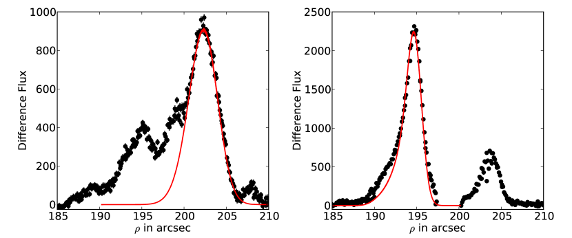
Figure 4.— Observed LE profiles and corresponding best-fit models (red line) for LE113 (left) and LE117 (right). The larger width and symmetric shape of the LE113 profile on the sky is due to the dust filament being inclined $\sim 50^{\circ}$ closer to the tangential to the line-of-sight than the LE117 dust filament, compressing the entire lightcurve on the sky and resulting in a more symmetric point-like LE profile.

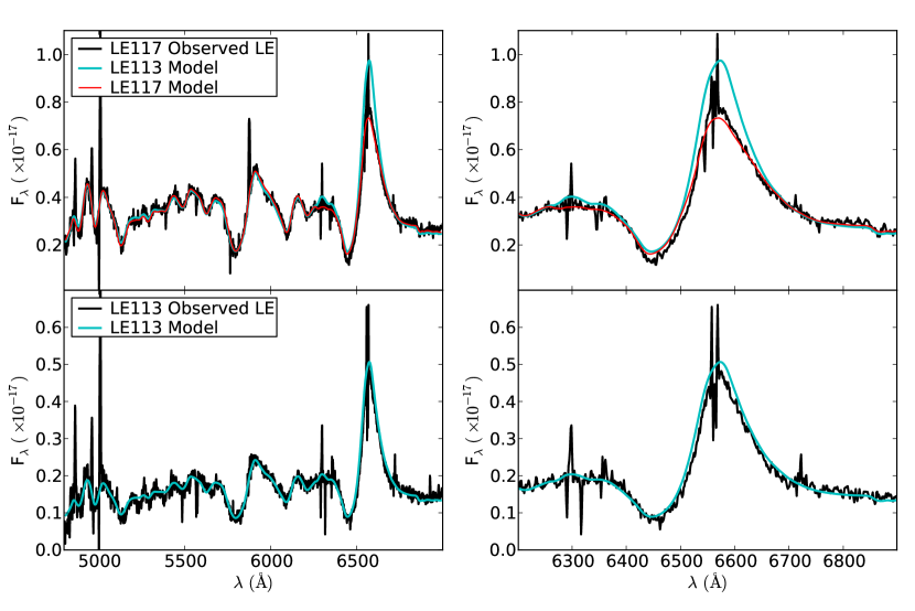
Figure 5.— The upper left panel shows the observed LE spectrum of LE117 with its corresponding isotropic model, along with the incorrect model of the nearby dust filament LE113. Only the matching LE117 model can fit the observed LE spectrum, while the lower left panel shows the LE113 observed LE spectrum can be fit with its corresponding model. The right panels show enlargements of the H$\alpha$ profile in both cases.

Table 1

LE ID	PA	$z_{0}$	$\theta$	$\alpha$	$\sigma_{d}$	$\Delta\rho_{\rm offset}$	Epochs
	(∘ )	(ly)	(∘ )	(∘ )	(ly)	(′′ )	(days)
LE016	15.8	428.91	17.1	22 $\pm$ 6	4.49 $\pm$ 0.03	-0.35	0-180
LE029	29.2	473.13	16.3	28 $\pm$ 2	4.49 $\pm$ 0.03	-0.19	5-200
LE032	31.8	483.02	16.2	-46 $\pm$ 2	2.71 $\pm$ 0.05	-0.27	30-180
LE034	33.9	486.53	16.1	-16 $\pm$ 2	3.37 $\pm$ 0.15	+0.26	0-140
LE053	53.0	505.05	15.8	38 $\pm$ 7	5.26 $\pm$ 0.03	-0.18	0-215
LE066	66.3	590.39	14.7	11 $\pm$ 2	4.50 $\pm$ 0.55	+1.05	0-80
LE069	69.3	624.64	14.3	66.8 $\pm$ 0.2	1.80 $\pm$ 0.07	+0.57	0-110
LE076	76.4	648.50	14.0	11 $\pm$ 4	0.60 $\pm$ 0.22	-0.08	40-135
LE113	112.5	671.04	13.8	79 $\pm$ 1	3.06 $\pm$ 0.09	-0.39	0-330
LE117	116.8	618.40	14.3	33 $\pm$ 5	3.10 $\pm$ 0.39	-0.14	35-155
LE180	180.2	289.69	20.7	-49 $\pm$ 2	4.53 $\pm$ 0.06	+0.73	0-290
LE186	185.6	270.34	21.3	70 $\pm$ 3	3.52 $\pm$ 0.18	-1.00	0-420
LE325	325.3	369.67	18.4	-6 $\pm$ 11	1.13 $\pm$ 0.16	+0.18	20-120
LE326	326.1	370.33	18.4	15 $\pm$ 3	2.24 $\pm$ 0.51	+0.21	0-130

3.2.2 Observation-Dominated Scenario

Here we consider a scenario where the properties of the observation (specifically the slit location) are the dominant factors in two very different observed LE spectra that have similar viewing angles onto the photosphere. Figure 6 shows the LE profiles of LE053 and LE066, corresponding to the slits at PA$\sim 60^{\circ}$ in Figure 1. The gray shaded region indicates the location of the slit for both profiles. The slit of LE066 was placed $\sim 1\hbox{${}^{\prime\prime}$}\,$ farther away from the SNR than the peak of the LE. This was unintentional since the location of the LE peak may not be very well known when making the MOS masks. The offset results in very different observed LE spectra for the two profiles, as shown in Figure 7. When compared to the observed LE spectra of Figure 5 and LE053 in Figure 7, the spectrum of LE066 looks more like an early-time spectrum with a lower H$\alpha$ emission-to-absorption ratio and a higher temperature continuum. Since the slit is centered on the pre-maximum light portion of the LE profile, LE066 does not probe epochs $>100$ days after maximum light, while LE053 probes epochs out to $\sim 300$ days after maximum light. As in the previous example, both model isotropic spectra are good fits to their observed LE spectra. However, the model of LE053 has a lower H$\alpha$ absorption velocity and a larger H$\alpha$ emission-to-absorption ratio, making it a poor fit to the LE066 observed LE spectrum.

The above dust- and observation-dominated examples highlight the danger in comparing LE spectra without sufficient modeling. Without the corresponding models for the LE053 and LE066 observed spectra, one might make a false-detection of asymmetry: the LE066 spectrum has a larger H$\alpha$ velocity and excess in emission compared to the LE053 spectrum. If the two LEs occurred at opposite PAs this asymmetry claim would be even more tempting to make.

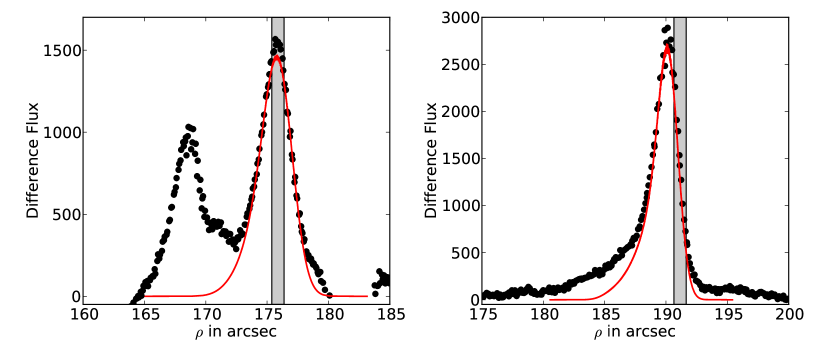
Figure 6.— Observed LE profiles and corresponding best-fit models (red line) for LE053 (left) and LE066 (right). The grey shaded regions indicate the location of the spectroscopic slit. The slit offset from the LE peak in the LE066 LE produces an observed spectrum that is heavily weighted towards the earlier epochs of the outburst.

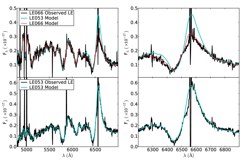
Figure 7.— The upper left panel shows the observed LE spectrum of LE066 with its corresponding isotropic model, along with the incorrect model of the nearby dust filament LE053. Only the higher velocity LE066 early-epoch model is a good fit for the observed LE spectrum. The lower left panel shows the LE053 observed LE spectrum which probes later epochs of the explosion. The lower velocity and larger H$\alpha$ emission-to-absorption ratio of the LE053 model is a good fit to the observed spectrum. The right panels show enlargements of the H$\alpha$ profile in both cases.

3.3. Evidence for Asymmetry in SN 1987A

Each PA on the LE system of SN 1987A represents a distinct viewing angle with which to view the original outburst. LEs originating to the north of SN 1987A probe outburst light originating mainly from the northern portion of the photosphere. Therefore, by observing the LEs as a function of increasing PA, we are able to view the outburst of SN 1987A as a function of north to south lines of sight. The scattering angles probed by the LE ring are listed in Table 1 and lead to typical opening angles of $\sim 35^{\circ}-40^{\circ}$.

Observed LE spectra and corresponding dust-modeled isotropic spectra are plotted as a function of PA in Figures 8-12, with each figure representing a field as shown in Figure 1. Figure 8 corresponds to the most northern field. As previously mentioned, we should avoid searching for differences between observed LE spectra. Instead, deviations in asymmetry are defined by deviations from the dust-modeled isotropic spectrum (red line) for each line of sight. A deviation from the model then describes a deviation from the appropriate weighted set of outburst spectra of SN 1987A as it was historically observed along the direct line of sight.

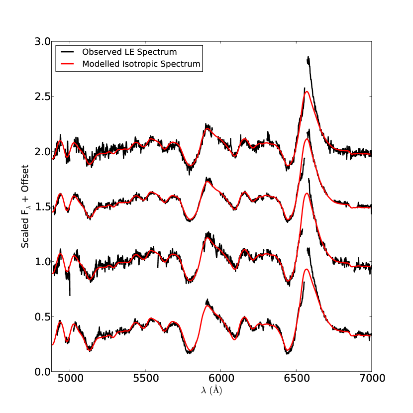
Figure 8.— Observed LE spectra with corresponding modeled isotropic spectra for field at PA $\sim 30\hbox{${}^{\circ}$}\,$ in Figure 1. Spectra are plotted from top to bottom as a function of increasing position angle as shown in Figure 1: LE016, LE029, LE032, LE034. Gaps in the observed spectra correspond to areas contaminated by sky-subtraction residuals.

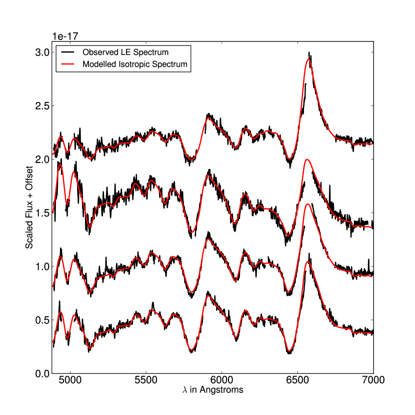
Figure 9.— Observed LE spectra with corresponding modeled isotropic spectra for field at PA $\sim 65\hbox{${}^{\circ}$}\,$ in Figure 1. Spectra are plotted from top to bottom as a function of increasing position angle as shown in Figure 1: LE053, LE066, LE069, LE076. Gaps in the observed spectra correspond to areas contaminated by sky-subtraction residuals.

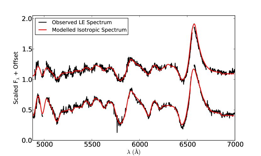
Figure 10.— Observed LE spectra with corresponding modeled isotropic spectra for field at PA $\sim 115\hbox{${}^{\circ}$}\,$ in Figure 1. Spectra are plotted from top to bottom as a function of increasing position angle as shown in Figure 1: LE113, LE117. Gaps in the observed spectra correspond to areas contaminated by sky-subtraction residuals.

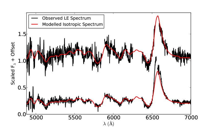
Figure 11.— Observed LE spectra with corresponding modeled isotropic spectra for field at PA $\sim 185\hbox{${}^{\circ}$}\,$ in Figure 1. Spectra are plotted from top to bottom as a function of increasing position angle as shown in Figure 1: LE180, LE186. Gaps in the observed spectra correspond to areas contaminated by sky-subtraction residuals. LE180 (upper spectrum) represents an example where our LE fitting algorithms fail to extract meaningful results due to the complexity and low signal-to-noise of both the spectrum and the LE flux profile.

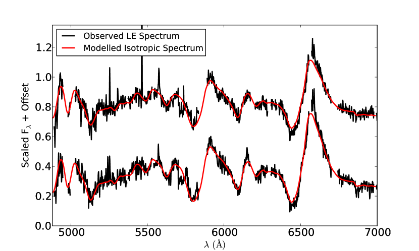
Figure 12.— Observed LE spectra with corresponding modeled isotropic spectra for field at PA $\sim 325\hbox{${}^{\circ}$}\,$ in Figure 1. Spectra are plotted from top to bottom as a function of increasing position angle as shown in Figure 1: LE325, LE326. Gaps in the observed spectra correspond to areas contaminated by sky-subtraction residuals.

3.3.1 H$\alpha$ Profiles

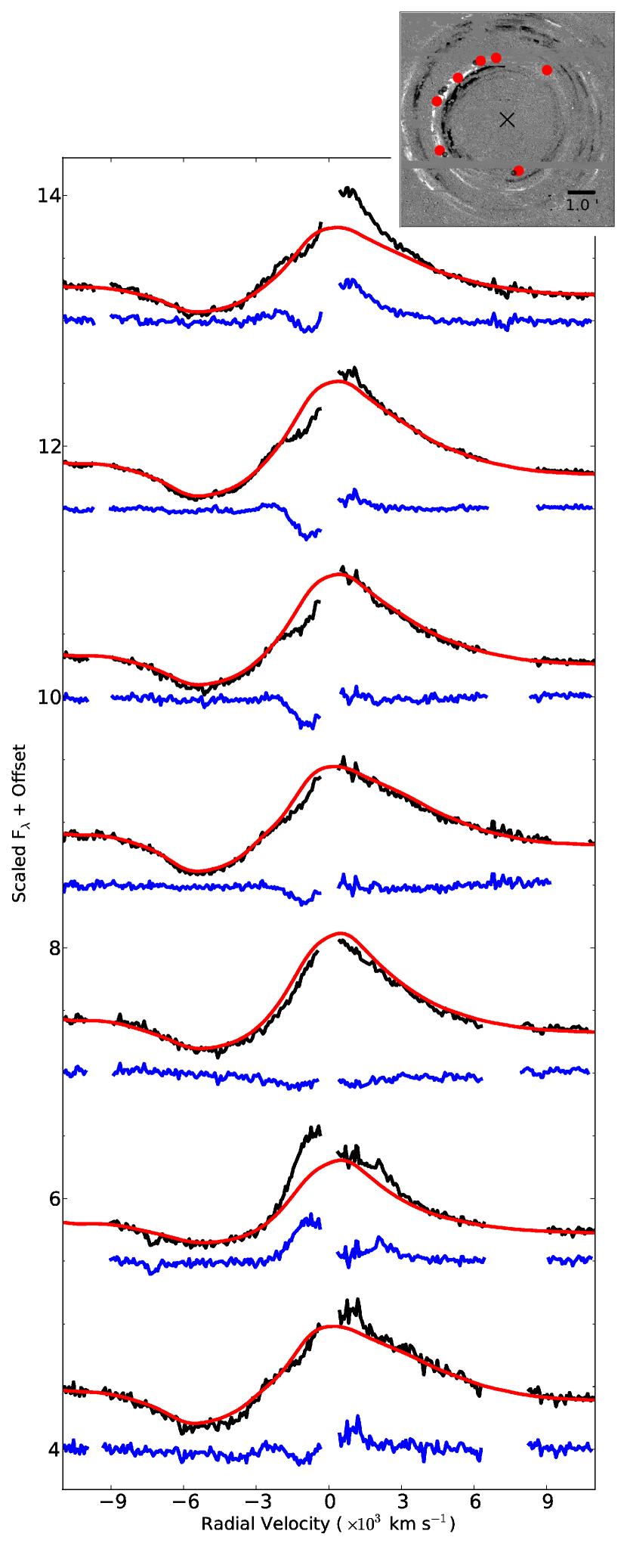
Figure 13.— Closeup of observed H$\alpha$ profiles (black) and corresponding dust-modeled isotropic spectra (red), as a function of PA for seven viewing angles. The top H$\alpha$ profile corresponds to the most northern slit in the upper right legend, and the profiles increase in PA from top to bottom: LE016, LE029, LE053, LE076, LE113, LE186, LE326. LE naming convention corresponds to PA of LE with respect to SNR. Residuals between the observed LE spectra and the dust-modeled isotropic spectra are plotted in blue below each profile. To prevent guiding the eye, the portions of the H$\alpha$ profile containing residuals from sky subtraction have been masked out. The most northern profile, LE016, has an excess in redshifted H$\alpha$ emission and a blue knee at $\sim-2000$ km s^-1 are observed. At almost opposite PA (LE0186, second from bottom), the opposite asymmetry is observed in the H$\alpha$ profile: an excess in blueshifted emission and a red knee at $\sim+2200$ km s^-1 . Both asymmetry features diminish as a function of viewing angle away from the north. Portions of the observed H$\alpha$ peak contaminated by sky-subtraction residuals have been removed to prevent guiding the eye. No smoothing has been applied to any of the spectra.

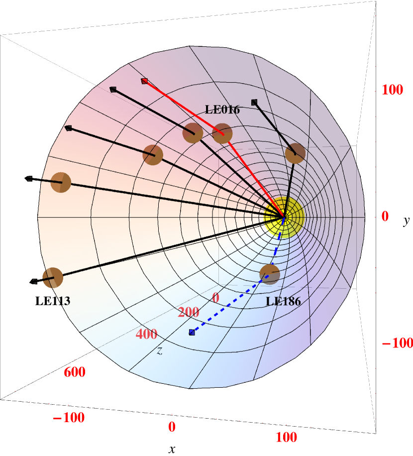
Figure 14.— 3D locations of the scattering dust for the seven LEs from Figure 13. Highlighted in solid red and dashed blue are the extreme viewing angles corresponding to LE016 and LE186. North is towards the positive $y$ axis, east is towards the negative $x$ axis, and $z$ is the distance in front of the SN. All units are in light years.

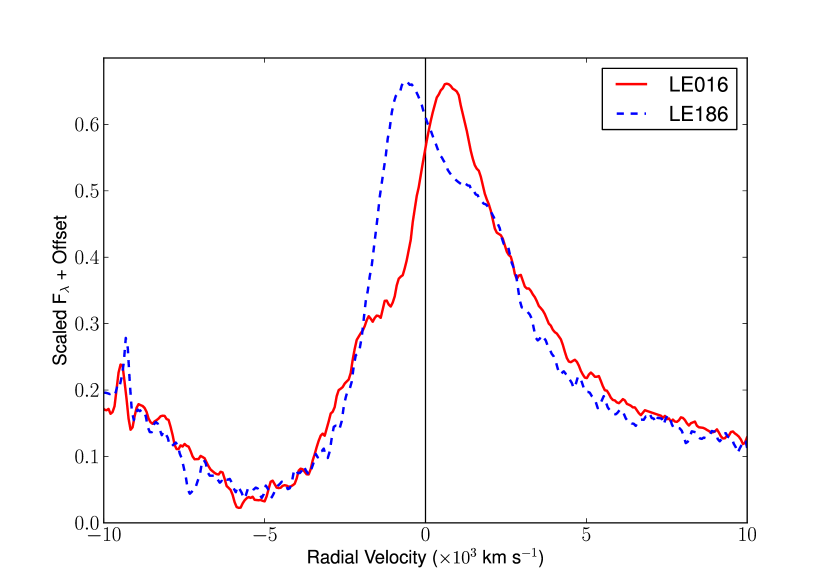
Figure 15.— Observed H$\alpha$ lines from LE016 and LE186. Emission peaks have been interpolated with high-order polynomials. Spectra are scaled and offset for comparison purposes, as well as smoothed with a boxcar of 3 pixels. Although this plot does not take into account the important differences in LE time-integrations between the spectra, it highlights the overall difference in fine-structure in the two LE spectra from opposite PAs. Observing H$\alpha$ profiles with opposite asymmetry structure at opposite PAs is surprising considering the opening angle between the two LEs is $<40^{\circ}$.

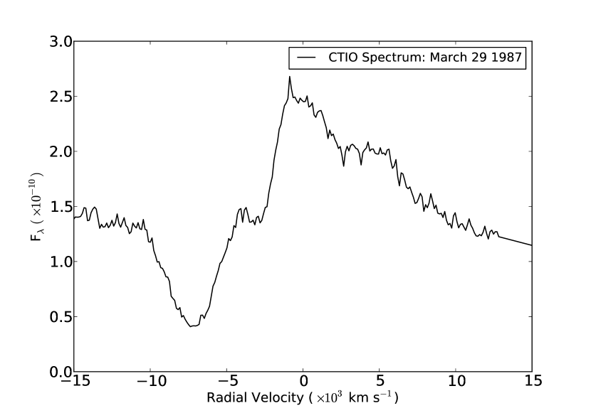
Figure 16.— Historical CTIO H$\alpha$ profile from Phillips et al. (1988) of SN 1987A taken on March 29, 1987, 34 days after explosion. The fine-structure, showing blue and red features at $\sim\pm 3500$ km s^-1 , defines the “Bochum event” which was observed 20-100 days after explosion. Evidence for this fine structure is not present after the historical spectra are integrated with the LE scattering model (red lines in Figure 13). H$\alpha$ fine structure observed in the LE spectra in Figure 13 must therefore require stronger line profile asymmetry than the original “Bochum event” or the asymmetry must last for much longer than originally observed for SN 1987A.

Figures 8-12 show that most features and line strengths observed in the optical LE spectra can be fit with the isotropic historical spectrum of SN 1987A, without the need to invoke asymmetry in the outburst. However, the fine-structure and strength of the H$\alpha$ $\lambda 6563$ line show deviations from symmetry as a function of PA (i.e. viewing angle onto the SN).

Figure 13 shows a closeup of the H$\alpha$ profiles of seven unique viewing angles as a function of increasing PA from top to bottom (the geometry of the viewing angles is shown in Figure 14). The most northern line of sight LE, LE016, shows a strong blue knee in the profile at $\sim-2000$ km s^-1 in addition to a strong excess of emission that is redshifted from the rest wavelength by $\sim+800$ km s^-1 (and by $\sim+500$ km s^-1 compared to the historical spectrum). The most southern LE, LE186, has a PA almost directly opposite that of LE016. Its H$\alpha$ profile (second from bottom in Figure 13) shows a red knee in the fine-structure at $\sim+2200$ km s^-1 and an excess in emission shifted towards the blue by $\sim-500$ km s^-1 (and by $\sim-1000$ km s^-1 compared to the historical spectrum). The qualitative difference in the H$\alpha$ profile shape between the two extreme viewing angles, LE016 and LE186, is shown in Figure 15. This figure does not take into account the effects of the LE observations on the integrated spectra and so cannot be used as a direct comparison between the viewing angles. However, it does qualitatively describe the asymmetry in the fine-structure between the two viewing angles.

The two asymmetries in the H$\alpha$ profile (summarized in Figure 15) are the fine-structure, with a blue knee in the northern profiles and a red knee in the southern profile, as well as an excess of H$\alpha$ emission that is redshifted in the north and blueshifted in the south. Both of these asymmetries appear to be physical for a number of reasons. The excess in H$\alpha$ emission as well as the blue knee feature smoothly diminish in Figure 13 as PA is increased. At PA $\sim 110^{\circ}$ in the south-east quadrant, both the H$\alpha$ strength and fine-structure from LEs LE113 and LE117 can be fit with the historical model spectrum of SN 1987A. The fact that both H$\alpha$ asymmetries (fine-structure and redshifted emission) smoothly diminish as a function of viewing angle from north to south in the eastern half of the LE ring is strong evidence that these asymmetries are physical.

This fine-structure in the H$\alpha$ profile is similar to the “Bochum event” (named after the 61 cm Bochum telescope at La Silla, Chile) originally observed in SN 1987A (Hanuschik & Dachs, 1987; Phillips & Heathcote, 1989), where blue and red satellite emission features were observed 20-100 days after explosion. Figure 16 shows the H$\alpha$ profile of a CTIO spectrum taken 34 days after explosion (Phillips et al., 1988). The blue and red emission satellites are similar to the blue and red knees observed in the LE016 and LE186 LE spectra, respectively. It is tempting to compare the H$\alpha$ fine-structure observed in Figure 16 directly with the fine-structure observed in the LE profiles. However, LE spectra represent an integration of many epochs of signal and cannot be compared directly to a single epoch spectrum. Although the “Bochum event” is prominent in Figure 16, there is no evidence for fine-structure in any of the isotropic model spectra in Figure 13. That is, the “Bochum event” does not survive the smoothing effect when the historical spectra of SN 1987A are integrated. This can be seen in the lower panel of Figure 3, where the fine-structure from the “Bochum event” is faintly visible in the maximum light spectrum, but entirely nonexistent in the integrated model spectra. The fact that fine-structure similar to the “Bochum event” is present in the observed LE spectra is evidence for underlying fine-structure that is much stronger than that originally observed for SN 1987A. In general, small deviations from symmetry observed in a LE spectrum must represent very large deviations from symmetry in the underlying outburst in order to remain after the integrating effect of the LE phenomenon. This is an important aspect of all LE spectroscopy work that is rarely emphasized.

The excess emission in the north and south from profiles LE016 and LE186, respectively, cannot be explained within uncertainties. To obtain the largest temporal coverage we used both CTIO and SAAO spectra when integrating the model spectrum. There exists known systematic differences between the datasets of the original observations from the two locations (Hamuy et al., 1990). Using the two data sets individually in our analysis pipeline can lead to differences in the H$\alpha$ strength by $5\%-10\%$ in our models, but cannot account for the $30\%-40\%$ excess observed in the LE016 and LE186 spectra. We also stress that our analysis is based on relative flux comparisons only.

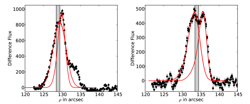
Figure 17.— LEFT: Observed LE profile on the sky for the southern LE186. Over-plotted in red are models for two scattering dust filaments which both contribute signal to the slit (plotted as the shaded region). Although the narrow filament at larger $\rho$ contributes late-time epochs to the spectrum, allowing for a larger emission-to-absorption ratio, the excess emission in the LE186 H$\alpha$ profile in Figure 13 cannot be modeled with the historical spectra of SN 1987A. See Appendix for full consideration. RIGHT: Observed LE profile of LE180. See Appendix for full consideration on why the LE fitting algorithm does not provide meaningful results in this complex case.

The LE profile on the sky for LE016 is very similar to that shown in Figure 3. Since it is a single peak, the theoretical maximum amount of H$\alpha$ emission in the model would correspond to integrating the historical spectra with the full lightcurve of SN 1987A out to $t=t_{now}$, rather than an effective lightcurve that is truncated by a window function (i.e. having an infinitely thick dust sheet). However, even this unphysical limit cannot reproduce the H$\alpha$ emission-to-absorption ratio that is seen in the observed LE profile of LE016. The LE profile on the sky and the slit location for LE186, which has two closely spaced filaments, are shown in Figure 17. Since the slit was placed on the first peak, there will be late-time nebular emission entering the slit from the second peak at larger $\rho$. In such a case, it is possible to obtain a larger emission-to-absorption ratio. However, we have taken this into account by modeling both LE peaks and determining the relative contributions from each peak entering the slits. This effect, discussed in more detail in the Appendix, cannot account for the excess in emission in LE186. We also stress that the apparent lack of any H$\alpha$ emission excess in LE180 is due to limitations in our LE fitting algorithrims when dealing with such low signal-to-noise data. LE180 is discussed in more detail in the Appendix. It should be noted, however, that LE180 appears to show the same fine-structure in H$\alpha$ (blueshifted emission peak and red knee) despite the low signal of the spectrum.

The opening angles probed by the LE lines of sight are $<45\hbox{${}^{\circ}$}\,$. The fact that large asymmetries are seen in the observed integrated LE spectra for relatively small changes in viewing angle is evidence for a strong asymmetry in the explosion.

3.3.2 Additional Evidence of Asymmetry

Although the H$\alpha$ profile shows the strongest asymmetry signature that is dependent on viewing angle, we note here two additional possible sources of asymmetry from the LE spectra: a velocity shift in the Fe II $\lambda 5018$ line that appears to be correlated with the H$\alpha$ asymmetry, and an unidentified feature near $5265$Å present in only one direction.

Figure 18.— Observed Fe II $\lambda 5018$ line in LE016 most-northern LE spectrum. The isotropic dust-modeled spectrum is over-plotted (solid red line), along with the same isotropic spectrum shifted $800$ km s^-1 to the red (dashed blue line), corresponding to the best fit to the peak location of the $\lambda 5018$ line and of similar magnitude to the velocity shift observed in the H$\alpha$ profile. Note that the velocity-shifted model spectrum is a better fit to the observed LE spectrum, indicating that the H$\alpha$ velocity asymmetry may be correlated with the velocity of the Fe II $\lambda 5018$ line.

Figure 18 plots the Fe II $\lambda 5018$ line for the observed LE spectra of LE016 (black), the asymmetric northern viewing angle. The dust-modeled isotropic spectrum is plotted as solid red. We also plot in dashed blue the same isotropic spectrum redshifted by $+800$ km s^-1 , which gives the best fit to the emission peak of the Fe II $\lambda 5018$ line (determined by eye). The redshifted spectrum is a better fit to the line and is consistent with the $600-800$ km s^-1 redshift observed in the H$\alpha$ line for the same viewing angle. As with the H$\alpha$ line asymmetry, the magnitude of the best-fitting redshift for the Fe II $\lambda 5018$ line decreases as a function of viewing angle away from the LE016 line of sight. For the case of LE186, the line is weak and heavily contaminated from sky residuals. Although it has the most blueward Fe II $\lambda 5018$ line of all observed LE spectra, it is unclear if the line is actually blueshifted with respect to the isotropic model or to zero. The structure is complicated since this line is part of a blend of the Fe II $\lambda\lambda 4924$, $5018$, $5169$ features.

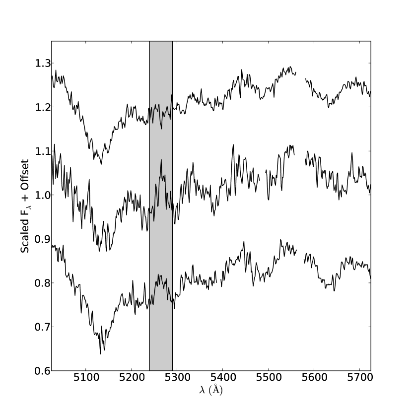
Figure 19.— Observed LE spectrum for LE016 (top) compared with the two “equatorial” LE locations (LE113 and LE117, middle and lower, respectively) shown at PA $\sim 115\hbox{${}^{\circ}$}\,$ in Figure 1. Both spectra show an unidentified feature near $5265$Å that is not present in any other viewing angle. The fact that the line appears broader in the upper spectrum is consistent with that LE probing a narrower range of early, high-velocity epochs compared to the lower spectrum as described in Section 3.2.1.

Figure 19 shows an unidentified feature near $5265$Å in the observed LE spectra for both “equatorial” (i.e. perpendicular to maximum asymmetry axes $16$^∘ /$186$^∘ ) lines of sight at PA $\sim 115\hbox{${}^{\circ}$}\,$. Many LE spectra have signal-to-noise ratios higher than the lower spectrum of Figure 19, however there is no evidence for the feature in any other line of sight. The fact that the feature is broader in the LE117 (lower) spectrum is consistent with that LE probing a narrower range of early, high-velocity epochs as described in Section 3.2.1. Considering this wavelength region is populated with many line blends and the fact that the spectra represent a time-integration, it is currently unclear if the feature is due to differences in chemical or velocity properties at this viewing angle.

4. Discussion

Ignoring the smaller knee-like fine-structure, the H$\alpha$ profiles of the LE016 and LE186 viewing angles in Figure 15 argue strongly for a one-sided asymmetry in SN 1987A. An overabundance of ⁵⁶Ni in the southern far hemisphere would create an excess in nonthermal excitation of hydrogen. This results in an excess in redshifted emission for the northern LE016 viewing angle. If the overabundance of ⁵⁶Ni is inclined close to the plane of the sky (within $21^{\circ}$), the overexcitation would occur in the near hemisphere with respect to the LE186 line of sight, explaining the blueshifted H$\alpha$ emission in LE186. The question remains if the asymmetry summarized in Figure 15 is strictly a result of this one-sided asymmetry plus time-integration effects, or if an additional asymmetry is the cause of the blue and red knee in the fine-structure of H$\alpha$ in LE016 and LE186, respectively.

The “Bochum event” (Figure 16) has previously been interpreted as an asymmetric distribution of ⁵⁶Ni (e.g., Lucy, 1988; Hanuschik & Thimm, 1990; Chugai, 1991a). Although both blue and red emission features are observed in Figure 16, the blue emission feature was only additionally observed in H$\beta$ (Hanuschik & Thimm, 1990) while the redshifted emission feature was also observed in infrared hydrogen lines (Larson et al., 1987) and [Fe II] lines (Haas et al., 1990). Chugai (1991a) proposed a two-sided ⁵⁶Ni asymmetry: (1) a dominant ⁵⁶Ni cloud in the far hemisphere producing the red emission fine-structure and the redshifted emission peak at later epochs, and (2) a smaller, higher velocity ⁵⁶Ni cloud in the near hemisphere producing the blue fine-structure. However, instead of invoking a smaller ⁵⁶Ni cloud in the near hemisphere, the more recent explanation for the blue fine-structure is a non-monotonic Sobolev optical depth, $\tau(v)$, for H$\alpha$ with a minimum near $v\approx 5000\hbox{$~{}$km$~{}$s${}^{-1}$}\,$ (Chugai, 1991b; Utrobin et al., 1995; Wang et al., 2002; Utrobin & Chugai, 2002, 2005). This interpretation does not require breaking spherical symmetry to explain the blue fine-structure. Although Utrobin & Chugai (2005) favor this scenario, their model cannot successfully produce the optical depth minimum at the required strength. The smooth transition of the H$\alpha$ profiles in PA from LE016 to LE117 in Figure 13 shows that the blue fine structure is dependent on viewing angle. As such, some form of deviation from spherical symmetry must be the root of the blue fine-structure in the LE H$\alpha$ profiles and presumably directly correlated to the blue fine-structure observed in the “Bochum event.”

The “Bochum event” was observed on days 20-100, while the redshift in lines of hydrogen and other elements was observed after $\sim 150$ days. For each LE spectrum, Table 1 lists the approximate range of epochs that contribute to the LE spectrum at greater than the $50\%$ level. This relative contribution is based on the window function generated for each LE (Figure 3), prior to any flux-weighted integration. While the temporal resolution in the LEs is not capable of distinguishing between photospheric and nebular epochs, we can compare LEs with different degrees of nebular emission. It is therefore interesting to note that both the fine-structure and the velocity shift of the H$\alpha$ line appear to be more dominantly a function of viewing angle rather than a function of epoch. LE066 probes the first $\sim 80$ days of the explosion only, but does not show fine-structure in H$\alpha$ considerably different than the nearby LEs probing much later epochs. The fact that the blue fine-structure feature is also present in the early-epoch LE066 spectrum almost certainly links this feature to an exaggerated version of the original “Bochum event.”

Since the H$\alpha$ P Cygni line is a blend with Ba II $\lambda 6497$, it is possible an asymmetry in the Ba II line is causing the observed blue fine-structure in the LE spectra. However, Utrobin et al. (1995) determined that the inclusion of the Ba II line was not sufficient to explain the blue emission in the “Bochum event.” Additionally, unlike H$\alpha$ , the Ba II $\lambda 6142$ line appears to be fit well with the isotropic model in the LE spectra.

A two-sided ⁵⁶Ni model such as Chugai (1991a) could explain the H$\alpha$ LE observations. A smaller high-velocity cloud blueshifted in the north causing the blue and red fine-structure in the north and south viewing angles, respectively. And a larger cloud redshifted in the south causing the red- and blue-shifted excess in the emission observed in the north and south viewing angles, respectively. The larger cloud could also be responsible for the Fe II asymmetry shown in Figure 18. The original observations of SN 1987A provided strong evidence for the large cloud being in the far hemisphere as previously stated. This is apparent in the isotropic model spectrum of LE186, where the time-integrated emission peak of H$\alpha$ is shifted to the red. LE186 probes a larger range of epochs in the explosion (out to $\sim 400$ days), so the redshift and integrated line profile asymmetry is most apparent in the LE186 isotropic model. The observed LE spectrum, however, shows a small blueshift with respect to zero velocity, implying the overabundance is inclined within $21^{\circ}$ of the plane of the sky in the southern far hemisphere. If the cloud was $\sim 20^{\circ}$ from the plane of the sky, the radial velocities would be a factor of $1.7-1.9$ larger in the north and south viewing angles, more easily altering the H$\alpha$ profile shape of the integrated LE spectra.

Figure 15 highlights the H$\alpha$ emission peak redshifted and blueshifted with respect to zero velocity in the northern (LE016) and southern (LE186) viewing angles, respectively. With respect to the isotropic model of SN 1987A, the absolute velocity shift of the H$\alpha$ peak is twice as large in the south ($-1000$ km s^-1 in LE186 compared to $+500$ km s^-1 in LE016). This is surprising considering both LEs have nearly equal $\sim 20^{\circ}$ north and south lines of sight onto the photosphere. However, LE186 probes over twice the range of epochs in the original explosion compared to LE016. The velocity shift is most likely more apparent at these later nebular epochs as previously discussed, potentially accounting for the larger velocity shift for LE186.

In addition to SN 1987A, a velocity shift in the H$\alpha$ peak or a Bochum-like event has also been observed for the Type IIP SNe SN 1999em, SN 2000cb, SN 2004dj, and SN 2006ov, as well as the Type II SN 2006bc (Elmhamdi et al., 2003; Kleiser et al., 2011; Chugai et al., 2005; Chornock et al., 2010; Gallagher et al., 2012). The H$\alpha$ profiles of SN 2004dj are strikingly similar to that of the LE186 profile in Figure 15. Although LE spectra cannot be compared directly with instantaneous spectra, it appears the H$\alpha$ lines from Chugai et al. (2005) would resemble that of LE186 after being smoothed by time-integration. Chugai et al. (2005) were able to successfully model the SN 2004dj H$\alpha$ fine-structure using an asymmetric bipolar ⁵⁶Ni distribution, including a spherical component with two cylindrical components. They modeled the observer viewing a dominant jet $30^{\circ}$ off-axis, resulting in a larger blueshifted emission peak with a smaller redshifted feature in the profiles of H$\alpha$ . This describes the LE186 LE profile in Figure 15, suggesting a bipolar ⁵⁶Ni distribution as a possible explanation. Since at the opposite PA, LE016, we see the opposite set of features in Figure 15, the two LE viewing angles would have to be looking towards opposite ends of the bipolar distribution in the model of Chugai et al. (2005). Since the viewing angles only differ by $\sim 40^{\circ}$, this would put strict constraints on the orientation of the bipolar distribution. This is, however, consistent with the dominant ⁵⁶Ni component being aligned within $\sim 20^{\circ}$ to the plane of the sky, as previously suggested.

 

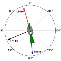
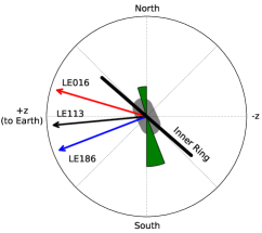
Figure 20.— LEFT: PAs on the sky of the three dominant LE viewing angles LE016, LE113 and LE186. The central grey region denotes the orientation on the sky of the elongated remnant ejecta (PA = $16^{\circ}$) from Kjær et al. (2010). The green wedges illustrate the proposed two-sided distribution of ⁵⁶Ni, most dominant in the southern hemisphere. White circles illustrate the locations of the two mystery spots as identified by Nisenson & Papaliolios (1999), with radius proportional to relative brightness in magnitudes of the two sources. Only the relative distance from the center of the SNR to the mystery spots is to scale in the image. RIGHT: Schematic with viewing angle perpendicular to Earth’s line of sight. The inclination of the inner circumstellar ring is shown along with the proposed two-sided distribution of ⁵⁶Ni in green. Note that the green wedges are to highlight the proposed geometry (not absolute velocity) of the ⁵⁶Ni asymmetry probed by the LE spectra, illustrating that the southern overabundance is most dominant.

As noted in the introduction, one of the benefits of LE spectroscopy is it allows the signatures of the explosion in the first few hundred days to be compared directly with the state of the remnant. The PA of the symmetry axis of the elongated ejecta was measured to be $14^{\circ}\pm 5^{\circ}$ using HST imaging (Wang et al., 2002) and $15^{\circ}\pm 0.9^{\circ}$ using IFU spectra (Kjær et al., 2010). This PA corresponds to LE016, where we see the maximum deviation from symmetry in H$\alpha$ in the northern hemisphere. Kjær et al. (2010) found the present-day ejecta to be blueshifted in the north and redshifted in the south, inclined out of the plane of the sky by $\sim 25^{\circ}$. The bipolar ⁵⁶Ni distribution proposed above to explain the LE observations is therefore aligned with the roughly $25$ year-old ejecta both in PA and inclination out of the sky. The inner ring of circumstellar material is inclined $49^{\circ}$ out of the plane of the sky, blueshifted in the north (Sugerman et al., 2005). The outer circumstellar rings are similarly inclined, presumably related to the rotation axis of the progenitor. The elongated ejecta and ⁵⁶Ni distribution probed by the LE observations are therefore aligned approximately in plane with the equatorial ring, as opposed to sharing a symmetry axis as initially proposed by Wang et al. (2002). This disfavors the axially symmetric jet-induced explosion model for SN 1987A proposed by Wang et al. (2002). We illustrate the proposed asymmetry with a schematic in Figure 20, highlighting the overabundance of ⁵⁶Ni close to the plane of the sky and redshifted in the southern hemisphere.

The “mystery spot” of SN 1987A was a bright source observed in speckle interferometry measurements 30, 38, and 50 days after the explosion, separated by only 60 mas from the SN (Nisenson et al., 1987; Meikle et al., 1987), and appearing at PA=$194^{\circ}\pm 2^{\circ}$. Nisenson & Papaliolios (1999) reprocessed this data, and identified two mystery spots in the data: (1) the original bright source at PA=$194^{\circ}\pm 3^{\circ}$ separated by $60\pm 8$ mas from the SNR, and (2) a fainter source at PA=$14^{\circ}\pm 3^{\circ}$ separated by $160\pm 8$ mas from the SNR. In order to be associated with the SN, they claimed the mystery spots must be at relativistic speeds with the northern spot blueshifted. A satisfactory explanation of the mystery spot (or spots) has yet to appear, a fact which is often forgotten. Figure 20 highlights the location of the mystery spots of Nisenson & Papaliolios (1999) with respect to our LEs. Since the PAs for the LE H$\alpha$ spectra showing maximum asymmetry ($16^{\circ}/186^{\circ}$) match the mystery spot PAs to within $10^{\circ}$, future modeling of the LE lines may aid in an explanation of the mystery spots.

If in fact the blue fine-structure of the “Bochum event” is due to an asymmetrical ⁵⁶Ni feature in the northern hemisphere, as the LE spectra here suggest, ⁵⁶Ni is transported to even higher velocities than previously considered. The blue feature emerges after 20 days at a radial velocity of $-5000\hbox{$~{}$km$~{}$s${}^{-1}$}\,$ in the H$\alpha$ profile. Since the blue fine-structure is most dominant in LE016 at a scattering angle of $17^{\circ}$, the lower limit of the absolute velocity of the ⁵⁶Ni cloud in the near hemisphere is $5200\hbox{$~{}$km$~{}$s${}^{-1}$}\,$, a velocity difficult to explain in current neutrino-driven explosion models. Absolute velocities of $>7000\hbox{$~{}$km$~{}$s${}^{-1}$}\,$ are required if the cloud is inclined within $45^{\circ}$ to the plane of the sky and upwards of $10000\hbox{$~{}$km$~{}$s${}^{-1}$}\,$ if within $30^{\circ}$. Assuming the dominant southern ⁵⁶Ni overabundance (and change in H$\alpha$ peak velocity) is correlated to the red emission feature observed in the “Bochum event” requires absolute velocities of $\sim 10000\hbox{$~{}$km$~{}$s${}^{-1}$}\,$ for that feature for an inclination of $20^{\circ}$ out of the plane of the sky. For the case of SN 2000cb, Utrobin & Chugai (2011) required radial mixing ⁵⁶Ni to velocities of $8400\hbox{$~{}$km$~{}$s${}^{-1}$}\,$ to reproduce the observed lightcurve of SN 2000cb, although it was a more energetic Type IIP than SN 1987A. Therefore, these unrealistically high velocities of ⁵⁶Ni for current neutrino-powered core-collapse explosion models require us to step back and view the asymmetries in Figure 15 at their most basic level: a non-spherical excitation structure in the early ejecta. Dessart & Hillier (2011) demonstrated that the P Cygni line profiles from non-spherical Type II ejecta can be altered significantly depending on viewing angle. Only future modeling of the LE spectra, taking into account the effects of time-integration, will allow the ejecta geometry to be determined or further constrained.

5. Conclusions

We have obtained optical spectra from the LE system of SN 1987A, allowing time-integrated spectra of the first few hundred days of the original explosion to be viewed from multiple lines of sight. We have modeled the LE spectra using the original photometry and spectroscopy of SN 1987A using the model of Rest et al. (2011a). Using specific examples we have showed the model correctly interprets LE flux profiles and spectra when both scattering dust properties and observational properties are taken into consideration.

Each PA on the LE system represents a unique viewing angle onto the photosphere which can be spectroscopically compared to the isotropic spectrum calculated from the original outburst of SN 1987A. The LE spectra show evidence for asymmetry, demonstrating the technique of targeted LE spectroscopy as a useful probe for observing SN asymmetries. The observed asymmetries can be summarized as follows:

1. Fine-structure in the H$\alpha$ line stronger than the original “Bochum event” is observed most strongly at PAs $16^{\circ}$ and $186^{\circ}$, with the H$\alpha$ profiles showing opposite asymmetry features in the north and south viewing angles.

2. At PA $16^{\circ}$ we observed an excess in redshifted H$\alpha$ emission and a blueshifted knee. At PA $186^{\circ}$ we observed an excess of blueshifted H$\alpha$ emission and a red knee. This fine-structure diminishes slowly as the PA increases from $16^{\circ}$ to $16^{\circ}+90^{\circ}$, with the LEs perpendicular to the symmetry axis showing no evidence for asymmetry.

3. At PA $16^{\circ}$ we observe a velocity shift in the Fe II $\lambda 5018$ line of the same magnitude and direction as the velocity shift in the H$\alpha$ emission peak at the same viewing angle. As with the H$\alpha$ fine-structure, this velocity shift appears to diminish as PA increases from $16^{\circ}$.

4. At PA $\sim 115^{\circ}$ (roughly perpendicular to symmetry axis defined by $16^{\circ}/186^{\circ}$ viewing angles) we observed an unidentified feature near $\lambda 5265$Å not observed in any other viewing angle.

This symmetry axis defined by the $16^{\circ}/186^{\circ}$ viewing angles is in excellent agreement with the current axis of symmetry in the ejecta geometry, the initial polarization and speckle observations, as well as the location of the “mystery spot.” The H$\alpha$ lines at PAs $16^{\circ}$ and $186^{\circ}$ are very similar to the H$\alpha$ lines observed in SN 2004dj and modeled as a two-sided ⁵⁶Ni distribution by Chugai et al. (2005). This same model could describe a two-sided ejection of ⁵⁶Ni in SN 1987A as probed by the LE H$\alpha$ lines. The ⁵⁶Ni is blueshifted in the north and redshifted in the south, with the dominant overabundance of ⁵⁶Ni being inclined $\sim 20^{\circ}$ from the plane of the sky. The indication that high-velocity ⁵⁶Ni is not correlated with the inner ring and presumed rotation axis may indicate that the explosion mechanism is independent of rotation. While these observations argue for a two-sided distribution of high-velocity ⁵⁶Ni, at their most basic level they probe unequal source functions of the H$\alpha$ line at different viewing angles. Only future modeling of the LE spectra will be able to constrain the early ejecta geometry with confidence.

Appendix A Effect of Dust Substructure in LE Profiles

For the observed LE profiles presented in this work, 11/14 show no strong evidence for dust substructure within the profile. These LE profiles can be modeled with one dust sheet effectively. However, LE113, LE180, and LE186 all show significant substructure in the their profiles (Figures 4 and 17) and we seek to quantify the effect this can have on the observed LE spectrum. Figures 21-23 show the observed LE profiles and the effect of dust substructure on the window functions and effective lightcurves. Figure 24 shows the differences in H$\alpha$ strengths obtained with and without including the effect of the secondary dust structure.

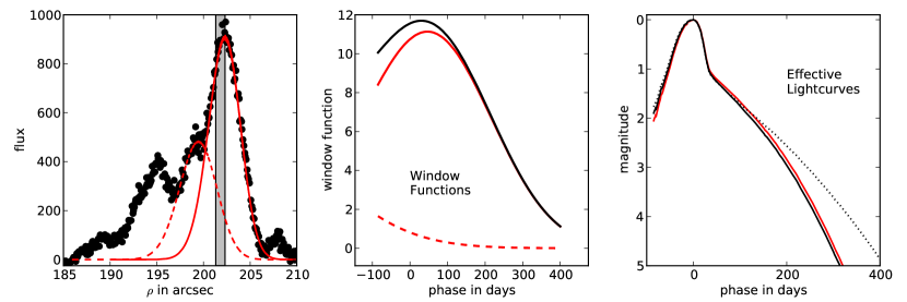
Figure 21.— LEFT: LE113 observed LE profile (black points) with the best fit to the primary dust sheet (solid red line), as well as the best fit to the secondary dust sheet (dashed red line). The location of the slit is shown with the grey region. MIDDLE: Window functions for the primary (solid red line) and secondary (dashed red line) dust sheets, as well as the total window function (solid black line). RIGHT: Effective lightcurves for the primary dust sheet (solid red line), the total effective lightcurve from both dust sheets (solid black line), and the original lightcurve of SN 1987A (dotted line). The effect of the secondary dust sheet is minimal in this case.

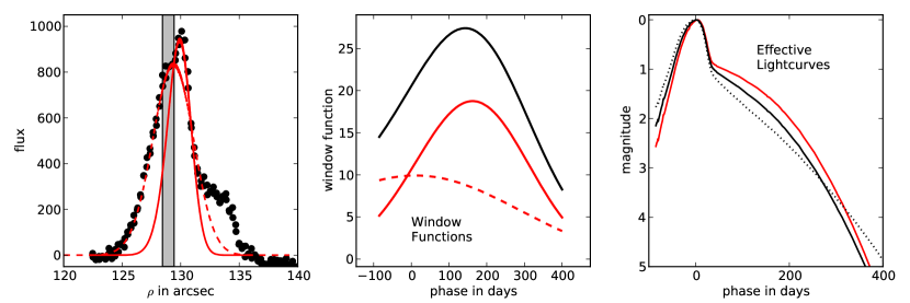
Figure 22.— LEFT: LE186 observed LE profile (black points) with the best fit to the primary dust sheet (solid red line), as well as the best fit to the secondary dust sheet (dashed red line). The location of the slit is shown with the grey region. MIDDLE: Window functions for the primary (solid red line) and secondary (dashed red line) dust sheets, as well as the total window function (solid black line). RIGHT: Effective lightcurves for the primary dust sheet (solid red line), the total effective lightcurve from both dust sheets (solid black line), and the original lightcurve of SN 1987A (dotted line). Without the secondary peak, the effective lightcurve is significantly biased towards later times due to the location of the slit. The secondary peak contributes flux from early epochs, reducing the late-epoch biased produced by the slit.

As shown in Figure 24, the effect of the secondary substructure on the resulting H$\alpha$ profile is minimal for LE113 ($<4\%$ difference in strength of emission peak), primarily because the flux contribution from the wing of the LE profile is so small. For LE186, including the secondary LE profile decreases the H$\alpha$ emission peak by $11\%$. Note, however, that because of the significant offset of the slit from the primary peak, the H$\alpha$ emission for LE186 is in excess of the full lightcurve-weighted integration of SN 1987A. For the case of LE180, the secondary peak significantly alters the window function and subsequent H$\alpha$ line, increasing the emission strength by $\sim 40\%$.

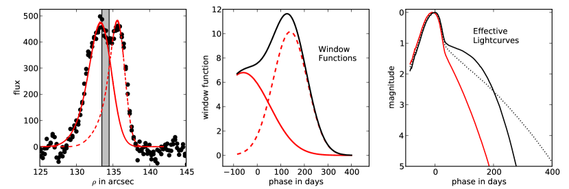
Figure 23.— LEFT: LE180 observed LE profile (black points) with the best fit to the primary dust sheet (solid red line), as well as the best fit to the secondary dust sheet (dashed red line). The location of the slit is shown with the grey region. MIDDLE: Window functions for the primary (solid red line) and secondary (dashed red line) dust sheets, as well as the total window function (solid black line). RIGHT: Effective lightcurves for the primary dust sheet (solid red line), the total effective lightcurve from both dust sheets (solid black line), and the original lightcurve of SN 1987A (dotted line). Here the two dust sheets create LE substructure with nearly equal amounts of flux. The window function in this case is significantly shifted to later times due to the presence of the secondary peak at larger values of $\rho$.

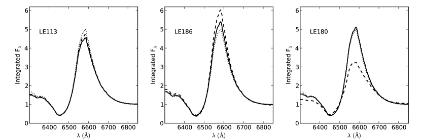
Figure 24.— Resulting H$\alpha$ profiles obtained by integrating the historical spectra of SN 1987A with the effective lightcurves in Figures 21-23 for LE113 (left panel), LE186 (middle panel), and LE180 (right panel). For each panel, the solid and dashed lines are from integrations of the total and primary-only effective lightcurves. The dotted line is H$\alpha$ profile obtained by integrating the actual lightcurve of SN 1987A with no window function truncating the integration.

Appendix B The Excess of H$\alpha$ Emission in LE186

The observed LE spectra and isotropic models for LE180 and LE186 in Figure 11 show two different results. LE186 shows a clear, high signal-to-noise excess in H$\alpha$ emission over the isotropic dust-modeled spectrum. LE180, probing essentially the same viewing angle onto the photosphere, does not show such an excess in the H$\alpha$ profile. In addition to the much lower signal-to-noise of LE180, we can use arguments based on the above dust substructure analysis to show that the excess emission observed in LE186 is physical.

As shown in the middle panel of Figure 24, the effect of the secondary LE peak in the LE186 profile is to reduce the emission peak of H$\alpha$ . The maximum amount of H$\alpha$ emission for LE186 therefore occurs when no secondary substructure is included. Since this gives an excess of only $\sim 10\%$, even this scenario is not able to account for the $\sim 30\%$ excess in H$\alpha$ in the observed LE186 spectrum.

For the case of LE180, the effect of the substructure is to increase the H$\alpha$ emission peak substantially ($\sim 40\%$ using the profile fits in Figure 23). Unlike the case of LE186, where the LE profile fits are well constrained within the data, the fits to the LE180 profile in Figure 23 are an example of a situation where our profile fitting algorithms cannot extract meaningful results due to the intrinsic complexity and low signal-to-noise ratio. It is most likely the case the secondary substructure in the LE180 profile is actually much wider than shown in Figure 23, which would result in more late-epoch contribution from the secondary peak and more emission in H$\alpha$ .

References

- Arnett et al. (1989) Arnett, W. D., Bahcall, J. N., Kirshner, R. P., & Woosley, S. E. 1989, ARA&A, 27, 629
- Bailey (1988) Bailey, J. 1988, Proceedings of the Astronomical Society of Australia, 7, 405
- Blondin et al. (2003) Blondin, J. M., Mezzacappa, A., & DeMarino, C. 2003, ApJ, 584, 971
- Burrows (2012) Burrows, A. 2012, ArXiv e-prints
- Caldwell et al. (1993) Caldwell, J. A. R., et al. 1993, MNRAS, 262, 313
- Catchpole et al. (1987) Catchpole, R. M., et al. 1987, MNRAS, 229, 15P
- Catchpole et al. (1988) —. 1988, MNRAS, 231, 75P
- Catchpole et al. (1989) —. 1989, MNRAS, 237, 55P
- Chornock et al. (2010) Chornock, R., Filippenko, A. V., Li, W., & Silverman, J. M. 2010, ApJ, 713, 1363
- Chugai (1991a) Chugai, N. N. 1991a, Soviet Ast., 35, 171
- Chugai (1991b) —. 1991b, Soviet Astronomy Letters, 17, 400
- Chugai et al. (2005) Chugai, N. N., Fabrika, S. N., Sholukhova, O. N., Goranskij, V. P., Abolmasov, P. K., & Vlasyuk, V. V. 2005, Astronomy Letters, 31, 792
- Cropper et al. (1988) Cropper, M., Bailey, J., McCowage, J., Cannon, R. D., & Couch, W. J. 1988, MNRAS, 231, 695
- Crotts (1988) Crotts, A. P. S. 1988, ApJ, 333, L51
- Dessart & Hillier (2011) Dessart, L., & Hillier, D. J. 2011, MNRAS, 415, 3497
- Elmhamdi et al. (2003) Elmhamdi, A., et al. 2003, MNRAS, 338, 939
- Gallagher et al. (2012) Gallagher, J. S., et al. 2012, ApJ, 753, 109
- Garg et al. (2007) Garg, A., et al. 2007, AJ, 133, 403
- Gawryszczak et al. (2010) Gawryszczak, A., Guzman, J., Plewa, T., & Kifonidis, K. 2010, A&A, 521, A38
- Gouiffes et al. (1988) Gouiffes, C., et al. 1988, A&A, 198, L9
- Haas et al. (1990) Haas, M. R., Erickson, E. F., Lord, S. D., Hollenbach, D. J., Colgan, S. W. J., & Burton, M. G. 1990, ApJ, 360, 257
- Hammer et al. (2010) Hammer, N. J., Janka, H.-T., & Müller, E. 2010, ApJ, 714, 1371
- Hamuy & Suntzeff (1990) Hamuy, M., & Suntzeff, N. B. 1990, AJ, 99, 1146
- Hamuy et al. (1990) Hamuy, M., Suntzeff, N. B., Bravo, J., & Phillips, M. M. 1990, PASP, 102, 888
- Hamuy et al. (1988) Hamuy, M., Suntzeff, N. B., Gonzalez, R., & Martin, G. 1988, AJ, 95, 63
- Hanuschik & Dachs (1987) Hanuschik, R. W., & Dachs, J. 1987, A&A, 182, L29
- Hanuschik & Thimm (1990) Hanuschik, R. W., & Thimm, G. J. 1990, A&A, 231, 77
- Jeffery (1987) Jeffery, D. J. 1987, Nature, 329, 419
- Kim et al. (2008) Kim, Y., Rieke, G. H., Krause, O., Misselt, K., Indebetouw, R., & Johnson, K. E. 2008, ApJ, 678, 287
- Kjær et al. (2010) Kjær, K., Leibundgut, B., Fransson, C., Jerkstrand, A., & Spyromilio, J. 2010, A&A, 517, A51
- Kleiser et al. (2011) Kleiser, I. K. W., et al. 2011, MNRAS, 415, 372
- Krause et al. (2008a) Krause, O., Birkmann, S. M., Usuda, T., Hattori, T., Goto, M., Rieke, G. H., & Misselt, K. A. 2008a, Science, 320, 1195
- Krause et al. (2008b) Krause, O., Tanaka, M., Usuda, T., Hattori, T., Goto, M., Birkmann, S., & Nomoto, K. 2008b, Nature, 456, 617
- Larson et al. (1987) Larson, H. P., Drapatz, S., Mumma, M. J., & Weaver, H. A. 1987, in European Southern Observatory Conference and Workshop Proceedings, Vol. 26, European Southern Observatory Conference and Workshop Proceedings, ed. I. J. Danziger, 147–151
- Lucy (1988) Lucy, L. B. 1988, in Supernova 1987A in the Large Magellanic Cloud, ed. M. Kafatos & A. G. Michalitsianos, 323–334
- Meaburn et al. (1995) Meaburn, J., Bryce, M., & Holloway, A. J. 1995, A&A, 299, L1
- Meikle et al. (1987) Meikle, W. P. S., Matcher, S. J., & Morgan, B. L. 1987, Nature, 329, 608
- Menzies et al. (1987) Menzies, J. W., et al. 1987, MNRAS, 227, 39P
- Miknaitis et al. (2007) Miknaitis, G., et al. 2007, ApJ, 666, 674
- Müller et al. (2012) Müller, B., Janka, H.-T., & Marek, A. 2012, ApJ, 756, 84
- Nisenson & Papaliolios (1999) Nisenson, P., & Papaliolios, C. 1999, ApJ, 518, L29
- Nisenson et al. (1987) Nisenson, P., Papaliolios, C., Karovska, M., & Noyes, R. 1987, ApJ, 320, L15
- Papaliolios et al. (1989) Papaliolios, C., Krasovska, M., Koechlin, L., Nisenson, P., & Standley, C. 1989, Nature, 338, 565
- Phillips et al. (1990) Phillips, M. M., Hamuy, M., Heathcote, S. R., Suntzeff, N. B., & Kirhakos, S. 1990, AJ, 99, 1133
- Phillips & Heathcote (1989) Phillips, M. M., & Heathcote, S. R. 1989, PASP, 101, 137
- Phillips et al. (1988) Phillips, M. M., Heathcote, S. R., Hamuy, M., & Navarrete, M. 1988, AJ, 95, 1087
- Rest et al. (2012a) Rest, A., Sinnott, B., & Welch, D. L. 2012a, Proceedings of the Astronomical Society of Australia, 29, 466
- Rest et al. (2011a) Rest, A., Sinnott, B., Welch, D. L., Foley, R. J., Narayan, G., Mandel, K., Huber, M. E., & Blondin, S. 2011a, ApJ, 732, 2
- Rest et al. (2005a) Rest, A., et al. 2005a, Nature, 438, 1132
- Rest et al. (2005b) —. 2005b, ApJ, 634, 1103
- Rest et al. (2008a) —. 2008a, ApJ, 681, L81
- Rest et al. (2008b) —. 2008b, ApJ, 680, 1137
- Rest et al. (2011b) —. 2011b, ApJ, 732, 3
- Rest et al. (2012b) —. 2012b, Nature, 482, 375
- Shigeyama & Nomoto (1990) Shigeyama, T., & Nomoto, K. 1990, ApJ, 360, 242
- Spyromilio et al. (1990) Spyromilio, J., Meikle, W. P. S., & Allen, D. A. 1990, MNRAS, 242, 669
- Sugerman et al. (2005) Sugerman, B. E. K., Crotts, A. P. S., Kunkel, W. E., Heathcote, S. R., & Lawrence, S. S. 2005, ApJS, 159, 60
- Suntzeff et al. (1988a) Suntzeff, N. B., Hamuy, M., Martin, G., Gomez, A., & Gonzalez, R. 1988a, AJ, 96, 1864
- Suntzeff et al. (1988b) Suntzeff, N. B., Heathcote, S., Weller, W. G., Caldwell, N., & Huchra, J. P. 1988b, Nature, 334, 135
- Utrobin (2004) Utrobin, V. P. 2004, Astronomy Letters, 30, 293
- Utrobin & Chugai (2002) Utrobin, V. P., & Chugai, N. N. 2002, Astronomy Letters, 28, 386
- Utrobin & Chugai (2005) —. 2005, A&A, 441, 271
- Utrobin & Chugai (2011) —. 2011, A&A, 532, A100
- Utrobin et al. (1995) Utrobin, V. P., Chugai, N. N., & Andronova, A. A. 1995, A&A, 295, 129
- van Dokkum (2001) van Dokkum, P. G. 2001, PASP, 113, 1420
- Wang & Wheeler (2008) Wang, L., & Wheeler, J. C. 2008, ARA&A, 46, 433
- Wang et al. (2002) Wang, L., et al. 2002, ApJ, 579, 671
- Weingartner & Draine (2001) Weingartner, J. C., & Draine, B. T. 2001, ApJ, 548, 296
- Whitelock et al. (1988) Whitelock, P. A., et al. 1988, MNRAS, 234, 5P
- Whitelock et al. (1989) —. 1989, MNRAS, 240, 7P
- Xu et al. (1995) Xu, J., Crotts, A. P. S., & Kunkel, W. E. 1995, ApJ, 451, 806