Bayesian Sparse Factor Analysis of Genetic Covariance Matrices

Abstract

Quantitative genetic studies that model complex, multivariate phenotypes are important for both evolutionary prediction and artificial selection. For example, changes in gene expression can provide insight into developmental and physiological mechanisms that link genotype and phenotype. However, classical analytical techniques are poorly suited to quantitative genetic studies of gene expression where the number of traits assayed per individual can reach many thousand. Here, we derive a Bayesian genetic sparse factor model for estimating the genetic covariance matrix (G-matrix) of high-dimensional traits, such as gene expression, in a mixed effects model. The key idea of our model is that we need only consider G-matrices that are biologically plausible. An organism’s entire phenotype is the result of processes that are modular and have limited complexity. This implies that the G-matrix will be highly structured. In particular, we assume that a limited number of intermediate traits (or factors, e.g., variations in development or physiology) control the variation in the high-dimensional phenotype, and that each of these intermediate traits is sparse – affecting only a few observed traits. The advantages of this approach are two-fold. First, sparse factors are interpretable and provide biological insight into mechanisms underlying the genetic architecture. Second, enforcing sparsity helps prevent sampling errors from swamping out the true signal in high-dimensional data. We demonstrate the advantages of our model on simulated data and in an analysis of a published Drosophila melanogaster gene expression data set.

Keywords G-matrix, factor model, sparsity, Bayesian inference, animal model

1 Introduction

Quantitative studies of evolution or artificial selection often focus on a single or a handful of traits at a time, such as size, survival or crop yield. Recently, there has been an effort to collect more comprehensive phenotypic information on traits such as morphology, behavior, physiology, or gene expression Houle (2010). For example, the expression of thousands of genes can be measured simultaneously Ayroles et al. (2009); Mcgraw et al. (2011); Gibson and Weir (2005), together capturing complex patterns of gene regulation that reflect molecular networks, cellular stresses, and disease states Xiong et al. (2012); de la Cruz et al. (2010), and may in some cases be important for fitness. Studying the quantitative genetics of multiple correlated traits requires a joint modeling approach Walsh and Blows (2009). However, applying the tools of quantitative genetics to high-dimensional, highly correlated datasets presents considerable analytical and computational challenges Meyer and Kirkpatrick (2010). In this paper we formulate a modeling framework to address these challenges for a basic component of quantitative genetic analysis: estimation of the matrix of additive genetic variances and covariances, or G-matrix Lynch and Walsh (1998). The G-matrix encodes information about responses to selection Lande (1979), evolutionary constraints Kirkpatrick (2009), and modularity Cheverud (1996), and is important for predicting evolutionary change Schluter (1996). Thus, G-matrix estimation is a key step for many quantitative genetic analyses.

The challenge in scaling classic methods to hundreds or thousands of traits is that the number of modeling parameters grows exponentially. An unconstrained G-matrix for $p$ traits requires $p(p+1)/2$ parameters, and modeling environmental variation and measurement error Kirkpatrick and Meyer (2004) requires at least as many additional parameters. Coupled with modest sample sizes, huge numbers of parameters can lead to instability in parameter estimates – analyses that are highly sensitive to outliers and have high variance. Previous methods for overcoming this instability include (1) “bending” or smoothing unconstrained estimates of G-matrices, such as from pairwise estimates of genetic covariation Ayroles et al. (2009); Stone and Ayroles (2009) or moments estimators Hayes and Hill (1981), and (2) estimating a constrained G-matrix to be low rank and thus specified with fewer parameters (e.g., Kirkpatrick and Meyer 2004). Constraining the G-matrix has computational and analytical advantages: fewer parameters result in more robust estimates and lower computational requirements Kirkpatrick and Meyer (2004). Constrained estimators of G-matrices include methods based on moments estimators Hine and Blows (2006); Mcgraw et al. (2011) and methods based on mixed effects models (e.g., the “animal model” and other related models Henderson (1984); Kruuk (2004); Kirkpatrick and Meyer (2004); de Los Campos and Gianola (2007). Mixed effects and related models have been particularly powerful for studies in large breeding programs and wild populations. These methods perform well on moderate-dimensional data. However, they are too computationally costly and not sufficiently robust to analyze high-dimensional traits.

Our objective in this paper is to develop a model for estimating G-matrices that is scalable to large numbers of traits and is applicable to a variety of experimental designs, including both experimental crosses and pedigreed populations. We build on the Bayesian mixed effects model of de Los Campos and Gianola (2007) and model the G-matrix with a factor model, but add additional constraints by using a highly informative, biologically-motivated, prior distribution. The key idea that allows us to scale to large numbers of traits is that the vast majority of the space of covariance matrices does not contain matrices that are biologically plausible as a G-matrix: we expect the G-matrix to be sparse, by which we mean that we favor G-matrices that are modular and low-rank. Sparsity in statistics refers to models in which many parameters are expected to be zero Lucas et al. (2006). By modular, we mean that small groups of traits will covary together. By low-rank, we mean that there will be few (important) modules. We call a G-matrix with these properties sparse because there exists a low-rank factorization (most of the possible dimensions are zero) of the matrix with many of its values equal to (or close to) zero. This constrains the class of covariance matrices that we search over, a necessary procedure for inference of covariance matrices from high-dimensional data Bickel and Levina (2008b, a); el Karoui (2008); Meyer and Kirkpatrick (2010); Carvalho et al. (2008); Hahn et al. (2013). Under these assumptions, we can also interpret the modules underlying our factorization without imposing additional constraints such as orthogonality Engelhardt and Stephens (2010), something not possible with earlier mixed effect factor models Meyer (2009).

The biological argument behind this prior assumption starts with the observation that the observed traits of an organism arise from common developmental processes of limited complexity, and developmental processes are often modular Cheverud (1996); Wagner and Altenberg (1996); Davidson and Levine (2008). For gene expression, regulatory networks control gene expression, and variation in gene expression can be often linked to variation in pathways Xiong et al. (2012); de la Cruz et al. (2010). For a given dataset, we make two assumptions about the modules (pathways): (1) a limited number of modules contribute to trait variation and (2) each module affects a limited number of traits. There is support and evidence for these modeling assumptions in the quantitative genetics literature as G-matrices tend to be highly structured Walsh and Blows (2009) and the majority of genetic variation is contained in a few dimensions regardless of the number of traits studied Ayroles et al. (2009); Mcgraw et al. (2011). Note that while we focus on developmental mechanisms underlying trait covariation, ecological or physiological processes can also lead to modularity in observed traits and our prior may be applied to these situations as well.

Based on these assumptions, we present a Bayesian sparse factor model for inferring G-matrices from pedigree information for hundreds or thousands of traits. We demonstrate the advantages of the model on simulated data and re-analyze gene expression data from a published study on Drosophila melanogaster Ayroles et al. (2009). Although high-dimensional sparse models have been widely used in genetic association studies Cantor et al. (2010); Engelhardt and Stephens (2010); Stegle et al. (2010); Parts et al. (2011); Zhou and Stephens (2012) to our knowledge, sparsity has not yet been applied to estimating a G-matrix.

2 Methods

In this section, we derive the Bayesian genetic sparse factor model as an extension to the classic multivariate animal model to the high-dimensional setting, where hundreds or thousands of traits are simultaneously examined. A factor model posits that a set of unobserved (latent) traits called factors underly the variation in the observed (measured) traits. For example, measured gene expression traits might be the downstream output of a gene regulatory network. Here, the activity of this gene network is a latent trait which might vary among individuals. We use the animal model framework to partition variation in both the measured traits and the latent factor traits into additive genetic variation and residuals. We encode our two main biological assumptions on the G-matrix as priors on the factors: sparsity in the number of factors that are important, and sparsity in the number of measured traits related to each factor. These priors constrain our estimation to realistic matrices and thus prevent sampling errors swamping out the true signal in high-dimensional data.

2.1 Model:

For a single trait the following linear mixed effects model is commonly used to explain phenotypic variation Henderson (1984):

$$\mathbf{y}_{i}=\mathbf{X}\mathbf{b}_{i}+\mathbf{Z}\mathbf{u}_{i}+\mathbf{e}_{i},$$ (1)

where $\mathbf{y}_{i}$ is the vector of phenotype measurements for trait $i$ on $n$ individuals; $\mathbf{b}_{i}$ is a vector of coefficients for the fixed effects and environmental covariates such as sex or age with design matrix $\mathbf{X}$; $\mathbf{u}_{i}\sim\mbox{N}(\mathbf{0},\sigma^{2}_{G_{i}}\mathbf{A})$ is the random vector of additive genetic effects with incidence matrix $\mathbf{Z}$, and $\mathbf{e}_{i}\sim\mbox{N}(\mathbf{0},\sigma^{2}_{R_{i}}\mathbf{I}_{n})$ is the residual error caused by non-additive genetic variation, random environmental effects, and measurement error. The residuals are assumed to be independent of the additive genetic effects. Here, $\mathbf{A}$ is the known $r\times r$ additive relationship matrix among the individuals; $r$ generally equals $n$, but will not if there are unmeasured parents, or if several individuals are clones and share the same genetic background (e.g., see the Drosophila gene expression data below).

In going from one trait to $p$ traits we can align the vectors $\mathbf{y}_{i}$ for each trait in (1) to form an $n\times p$ matrix $\mathbf{Y}$ specified by the following multivariate model:

$$\mathbf{Y}=\mathbf{XB}+\mathbf{ZU}+\mathbf{E},$$ (2)

where $\mathbf{B}=[\mathbf{b}_{1}\dots\mathbf{b}_{p}]$. $\mathbf{U}=[\mathbf{u}_{1}\dots\mathbf{u}_{p}]$ and $\mathbf{E}=[\mathbf{e}_{1}\dots\mathbf{e}_{p}]$ are random variables drawn from matrix normal distributions Dawid (1981):

$$\mathbf{U}\sim\mbox{MN}_{r,p}(\mathbf{0};\mathbf{A},\mathbf{G}),\quad\mathbf{E}\sim\mbox{MN}_{n,p}(\mathbf{0};\mathbf{I}_{n},\mathbf{R}),$$ (3)

where the subscripts $r,p$ and $n,p$ specify the dimensions of the matrices, $\mathbf{0}$ is a matrix of zeros of appropriate size, $\mathbf{A}$ and $\mathbf{I}_{n}$ specify the row (among individual) covariances for each trait, and $\mathbf{G}$ and $\mathbf{R}$ are the $p\times p$ matrices modeling genetic and residual covariances among traits within each individual.

We wish to estimate the covariance matrices $\mathbf{G}$ and $\mathbf{R}$. To do so, we assume that any covariance among the observed traits is caused by a number of latent factors. Specifically, we model $k$ latent traits that each linearly relate to one or more of the observed traits. We specify $\mathbf{U}$ and $\mathbf{E}$ via the following hierarchical factor model:

$$\begin{split}\mathbf{U}=\mathbf{F}_{a}\mathbf{\Lambda}^{T}+\mathbf{\Delta},&\quad\mathbf{E}=\mathbf{F}_{e}\mathbf{\Lambda}^{T}+\mathbf{\Xi}\\ \mathbf{F}_{a}\sim\mbox{MN}_{r,k}(\mathbf{0};\mathbf{A},\mathbf{\Sigma}_{a}),&\quad\mathbf{F}_{e}\sim\mbox{MN}_{n,k}(\mathbf{0};\mathbf{I}_{n},\mathbf{\Sigma}_{e})\\ \mathbf{\Delta}\sim\mbox{MN}_{r,p}(\mathbf{0};\mathbf{A},\mathbf{\Psi}_{a}),&\quad\mathbf{\Xi}\sim\mbox{MN}_{n,p}(\mathbf{0};\mathbf{I}_{n},\mathbf{\Psi}_{e})\\ \mathbf{\Lambda}&\sim\pi(\theta),\\ \end{split}$$ (4)

where $\mathbf{\Lambda}$ is a $p\times k$ matrix with each column characterizing the relationship between one latent trait and all observed traits. Just as $\mathbf{U}$ and $\mathbf{E}$ partition the among-individual variation in the observed traits into additive genetic effects and residuals in (2), the matrices $\mathbf{F}_{a}$ and $\mathbf{F}_{e}$ partition the among-individual variation in the latent traits into additive genetic effects and residuals. $\mathbf{\Sigma}_{a}$ and $\mathbf{\Sigma}_{e}$ model the within-individual covariances of $\mathbf{F}_{a}$ and $\mathbf{F}_{e}$, which we assume to be diagonal ($\mathbf{\Sigma}_{a}=\mbox{Diag}(\sigma^{2}_{a_{j}}),\mathbf{\Sigma}_{e}=\mbox{Diag}(\sigma^{2}_{e_{j}}))$. $\mathbf{\Psi}_{a}$ and $\mathbf{\Psi}_{e}$ are the idiosyncratic (trait-specific) variances of the factor model and are assumed to be diagonal.

In model (4), as in any factor model (e.g., West 2003), $\boldsymbol{\Lambda}$ is not identifiable without adding extra constraints. In general, the factors in $\boldsymbol{\Lambda}$ can be rotated arbitrarily. This is not an issue for estimating $\mathbf{G}$ itself, but prevents biological interpretations of $\boldsymbol{\Lambda}$ and makes assessing MCMC convergence difficult. To solve this problem, we introduce constraints on the orientation of $\boldsymbol{\Lambda}$ though our prior distribution $\pi(\theta)$ specified below, where $\theta$ is a set of hyperparameters. However, even after fixing a rotation, the relative scaling of corresponding columns of $\mathbf{F}_{a}$, $\mathbf{F}_{e}$ and $\boldsymbol{\Lambda}$ are still not well defined. For example, if the $j$th column of $\mathbf{F}_{a}$ and $\mathbf{F}_{e}$ are both multiplied by a constant $c$, the same model is recovered if the $j$th column of $\boldsymbol{\Lambda}$ is multiplied by $1/c$. To fix $c$, we require the column variances $\sigma^{2}_{a_{j}}$ and $\sigma^{2}_{e_{j}}$ to sum to one, i.e. $\mathbf{\Sigma}_{a}+\mathbf{\Sigma}_{e}=\mathbf{I}_{k}$. Therefore, the single matrix $\mathbf{\Sigma}_{h^{2}}=\mathbf{\Sigma}_{a}=\mathbf{I}_{k}-\mathbf{\Sigma}_{e}$ is sufficient to specify both variances. The diagonal elements of this matrix specify the narrow-sense heritability $(h^{2}_{j}=\frac{\sigma^{2}_{a_{j}}}{\sigma^{2}_{a_{j}}+\sigma^{2}_{e_{j}}}=\sigma^{2}_{a_{j}})$ of latent trait $j$.

Given the properties of the matrix normal distribution Dawid (1981) and models (3) and (4) we can recover $\mathbf{G}$ and $\mathbf{R}$ as:

$$\begin{split}\mathbf{G}&=\mathbf{\Lambda}\mathbf{\Sigma}_{h^{2}}\mathbf{\Lambda}^{T}+\mathbf{\Psi}_{a},\\ \mathbf{R}&=\mathbf{\Lambda}(\mathbf{I}_{k}-\mathbf{\Sigma}_{h^{2}})\mathbf{\Lambda}^{T}+\mathbf{\Psi}_{e}.\end{split}$$ (5)

Therefore, the total phenotypic covariance $\mathbf{P}=\mathbf{G}+\mathbf{R}$ is modeled as:

$$\mathbf{P}=\mathbf{\Lambda}\mathbf{\Lambda}^{T}+\mathbf{\Psi}_{a}+\mathbf{\Psi}_{e}.$$ (6)

Our specification of the Bayesian genetic sparse factor model in (4) differs from earlier methods such as the Bayesian genetic factor model of de Los Campos and Gianola (2007) in two key respects:

First, in classic factor models, the total number of latent traits is assumed to be small ($k\ll p$). Therefore, equation (5) would model $\mathbf{G}$ with only $pk+k+p$ parameters instead of $p(p+1)/2$. However, choosing $k$ is a very difficult, unsolved problem, and inappropriate choices can result in highly biased estimates of $\mathbf{G}$ and $\mathbf{R}$ (e.g, Meyer and Kirkpatrick 2008). In our model we allow many latent traits but assume that the majority of them are relatively unimportant. This subtle difference is important because it removes the need to accurately choose $k$, instead emphasizing the estimation of the magnitude of each latent trait. This model is based on the work by Bhattacharya and Dunson (2011), which they term an “infinite” factor model. In our prior distribution on the factor loadings matrix $\mathbf{\Lambda}$ (see section Priors), we order the latent traits (columns of $\mathbf{\Lambda}$) in terms of decreasing influence on the total phenotypic variation, and assume that the variation explained by these latent traits decreases rapidly. Therefore, rather than attempt to identify the correct $k$ we instead model the decline in the influence of successive latent traits. As in other factor models, to save computational effort we can truncate $\mathbf{\Lambda}$ to include only its first $k^{*}<k$ columns because we require the variance explained by each later column to approach zero. The truncation point $k^{*}$ can be estimated jointly while fitting the model and is flexible (we suggest truncating any columns of $\mathbf{\Lambda}$ defining a module that does not explain $>1\%$ of the phenotypic variation in at least 2 observed traits). Note that $k^{*}$ conveys little biological information and does not have the same interpretation as $k$ in classic factor models. Since additional factors are expected to explain negligible phenotypic variation, including a few extra columns of $\mathbf{\Lambda}$ to check for more factors is permissible (e.g., Meyer and Kirkpatrick 2008).

Second, we assume that the residual covariance $\mathbf{R}$ has a factor structure and that the same latent traits underly both $\mathbf{G}$ and $\mathbf{R}$. Assuming a constrained space for $\mathbf{R}$ is uncommon in multivariate genetic estimation. For example, de Los Campos and Gianola (2007) fit an unconstrained $\mathbf{R}$, although they used an informative inverse Wishart prior Gelman (2006) and only consider five traits. The risk of assuming a constrained $\mathbf{R}$ is that poorly modeled phenotypic covariance ($\mathbf{P}=\mathbf{G}+\mathbf{R}$) can lead to biased estimates of genetic covariance under some circumstances Jaffrezic et al. (2002); Meyer and Kirkpatrick (2008).

However, constraining $\mathbf{R}$ is necessary in high-dimensional settings to prevent the number of modeling parameters from increasing exponentially, and we argue that modeling $\mathbf{R}$ as we have done is biologically justified. Factor models fitting low numbers of latent factors are used in many fields because they accurately model phenotypic covariances. Reasonable constraints on $\mathbf{R}$ have been applied successfully in previous genetic models. One example is in the Direct Estimation of Genetic Principle Components model of Kirkpatrick and Meyer (2004). These authors model only the first $m_{E}$ eigenvectors of the residual covariance matrix. Our model for $\mathbf{R}$ is closely related to models used in random regression analysis of function-valued traits (e.g., Kirkpatrick and Heckman 1989; Pletcher and Geyer 1999; Jaffrezic et al. 2002; Meyer 2005). In those models, $\mathbf{R}$ is modeled as a permanent environmental effect function plus independent error. The permanent environmental effect function is given a functional form similar to (or more complex than) the genetic function. In equation (4), $\mathbf{F}_{e}$ is analogous to this permanent environmental effect (but across different traits rather than the same trait measured through time), with its functional form described by $\mathbf{\Lambda}$, and $\mathbf{\Xi}$ is independent error. Since both $\mathbf{F}_{a}$ and $\mathbf{F}_{e}$ relate to the observed phenotypes through $\mathbf{\Lambda}$, the functional form of the residuals ($\mathbf{e}_{i}$) in our model is at least as complex as the genetic functional form (and more complex whenever $h^{2}_{j}=0$ for some factors).

The biological justification of our approach is that the factors represent latent traits, and just like any other trait their value can partially be determined by genetic variation. For example, the activity of developmental pathways can have a genetic basis and can also be determined by the environment. The latent traits determine the phenotypic covariance of the measured traits, and their heritability determines the genetic covariance. In genetic experiments, some of these latent traits (e.g., measurement biases) might be variable, but not have a genetic component. We expect that some factors will contribute to $\mathbf{R}$ but not $\mathbf{G}$, so $\mathbf{R}$ will have a more complex form Meyer and Kirkpatrick (2008).

We examine the impact of our prior on $\mathbf{R}$ through simulations below. When our assumptions regarding $\mathbf{R}$ do not hold, the prior will likely lead to biased estimates. For example, measurement biases might be low-dimensional but not sparse. However, we expect that for many general high-dimensional biological datasets this model will be useful and can provide novel insights. In particular, by directly modeling the heritability of the latent traits, we can predict their evolution.

2.2 Priors:

Modeling high-dimensional data requires some prior specification or penalty/regularization for accurate and stable parameter estimation Hastie et al. (2003); West (2003); Poggio and Smale (2003). For our model this means that constraints on $\mathbf{G}$ and $\mathbf{R}$ are required. We impose constraints through highly informative priors on $\boldsymbol{\Lambda}$. Our priors are motivated by the biological assumptions that variation in underlying developmental processes such as gene networks or metabolic pathways give rise to to genetic and residual covariances.

This implies:
(1) The biological system has limited complexity: a small number of latent traits (e.g., developmental pathways) or measurement biases are relevant for trait variation. For the model this means that the number of factors retained in $\boldsymbol{\Lambda}_{k^{*}}$ is low ($k^{*}\ll p$).
(2) Each underlying latent trait affects a limited number of the observed traits. For the model this means the factor loadings (columns of $\boldsymbol{\Lambda}$) are sparse (mostly near zero).

We formalize the above assumptions by priors on $\boldsymbol{\Lambda}$ that impose sparsity (formally, shrinkage towards zero) and few highly influential latent traits Bhattacharya and Dunson (2011). This prior is specified as a hierarchical distribution on each element $\lambda_{ij}$ of $\boldsymbol{\Lambda}$:

$$\begin{split}\lambda_{ij}&\mid\phi_{ij},\tau_{j}\sim\mbox{N}\left(0,\phi_{ij}^{-1}\tau_{j}^{-1}\right),\;i=1\dots p,\;j=1\dots k\\ \phi_{ij}&\sim\mbox{Ga}(\nu/2,\nu/2),\\ \tau_{j}&=\prod\limits_{l=1}^{m}\delta_{l},\quad\delta_{1}\sim\mbox{Ga}(a_{1},b_{1}),\quad\delta_{l}\sim\mbox{Ga}(a_{2},b_{2})\mbox{ for }l=2\dots k.\end{split}$$ (7)

The hierarchical prior is composed of three levels: (a) We model each $\lambda_{ij}$ (which specifies how trait $i$ is related to latent trait $j$) with a normal distribution. Based on assumption (2), we expect most $\lambda_{ij}\approx 0$. A normal distribution with a fixed variance parameter is not sufficient to impose this constraint. (b) We model the the precision (inverse of the variance) of each loading element $\lambda_{ij}$ with the parameter $\phi_{ij}$ drawn from a gamma distribution. This normal-gamma mixture distribution (conditional on $\tau_{j}$) is commonly used to impose sparsity Tipping (2001); Neal (1996) as the marginal distribution on $\lambda_{ij}$ takes the form of a Student’s-t distribution with $\nu$ degrees of freedom and is heavy-tailed. The loadings are concentrated near zero, but occasional large magnitude values are permitted. This prior specification is conceptually similar to the widely-used Bayesian Lasso (Park and Casella 2008). (c) The parameter $\tau_{j}$ controls the overall variance explained by factor $j$ (given by: $\boldsymbol{\lambda}_{j}^{T}\boldsymbol{\lambda}_{j}$ where $\boldsymbol{\lambda}_{j}$ is the $j$th column of $\mathbf{\Lambda}$) by shrinking the variance towards zero as $m\rightarrow\infty$. The decay in the variance is enforced by increasing the precision on the normal distribution of each $\lambda_{ij}$ as $j$ increases so $|\lambda_{ij}|\rightarrow 0$. The sequence $\{\tau_{j}\}$ is formed from the cumulative product of $\{\delta_{1}\dots\delta_{k}\}$ each modeled with a gamma distribution, and will be stochastically increasing as long as $a_{2}>b_{2}$. This means that the variance of $\lambda_{ij}$ will stochastically decrease and higher-indexed columns of $\boldsymbol{\Lambda}$ will be less likely to have any large magnitude elements. This decay ensures that it will be safe to truncate $\boldsymbol{\Lambda}$ at some sufficiently large $k^{*}$ because columns $k>k^{*}$ will (necessarily) explain less variance.

The prior distribution on $\{\tau_{j}\}$ (and therefore $\{\delta_{1}\dots\delta_{k}\}$) is a key modeling decision as this parameter controls how much of the total phenotypic variance we expect each successive factor to explain. Based on assumption (1), we expect that few factors will be sufficient to explain total phenotypic variation, and thus $\{\tau_{j}\}$ will increase rapidly. However, relatively flat priors on $\{\delta_{2}\dots\delta_{k}\}$ (e.g., $a_{2}=3,b_{2}=1$), which allow some consecutive factors to be of nearly equal magnitude, appear to work well in simulations.

A discrete set of values in the unit interval were specified as the prior for the heritability of each of the common factor traits. This specification was selected for computational efficiency and to give $h^{2}_{j}=0$ positive weight in the prior. We find the following discrete distribution works well:

$$\pi(h^{2}_{j}=0)=0.5,\quad\pi(h^{2}_{j}=l/n_{h})=1/(2(n_{h}-1)),\mbox{ where }l=1\dots(n_{h}-1)$$ (8)

where $n_{h}$ is the number of points to evaluate $h^{2}_{j}$. In analyses reported here, we set $n_{h}=100$. This prior gives equal weight to $h^{2}_{j}=0$ and $h^{2}_{j}>0$ because we expect several factors (in particular, those reflecting measurement error) to have no genetic variance. In principle, we could place a continuous prior on the interval $[0,1]$, but no such prior would be conjugate, and developing a MCMC sampler would be more difficult.

We place inverse gamma priors on each element of the diagonals of the genetic and residual idiosyncratic variances: $\mathbf{\Psi}_{a}$ and $\mathbf{\Psi}_{e}$. Priors on each element of $\boldsymbol{\beta}$ are normal distributions with very large ($>10^{6}$ ) variances.

2.3 Implementation:

Inference in the above model uses an adaptive Gibbs sampler for which we provide detailed steps in the appendix. The code has been implemented in Matlab^® and can be found at the website (http://stat.duke.edu/$\sim$sayan/quantmod.html).

2.4 Simulations:

We present a simulation study of high-dimensional traits measured on the offspring of a balanced paternal half-sib breeding design. We examined ten scenarios (Table LABEL:table:simulation_setup), each corresponding to different models for the matrices $\mathbf{G}$ and $\mathbf{R}$ to evaluate the impact of the modeling assumptions specified by our prior. For each scenario we simulated parameters and trait values of individuals from model (2) with $\mathbf{Z}=\mathbf{I}_{n}$, $\mathbf{B}=\mathbf{0}_{p}$, and $\mathbf{X}$ a single column of ones representing the trait means.

Scenarios a-c were designed to test the ability of the model to accurately estimate $\mathbf{G}$ and $\mathbf{P}$ given 10, 25 or 50 important factors, respectively, for 100 traits. Latent factor traits $1\dots 5$, $1\dots 15$, or $1\dots 30$, respectively, were assigned a heritability ($h^{2}_{j}$) of 0.5 and contributed to both $\mathbf{G}$ and $\mathbf{R}$. The remaining factors ($6\dots 10$, $16\dots 25$, or $31\dots 50$, respectively) were assigned a heritability of 0.0 and only contributed to $\mathbf{R}$. To make the covariance matrices biologically reasonable, we chose each factor to be sparse: only 3-25 of the 100 traits were allowed to “load” on each factor. These loadings were drawn from standard normal distributions. The idiosyncratic variances $\boldsymbol{\Psi}_{a}$ and $\boldsymbol{\Psi}_{e}$ were set to $0.2\times\mathbf{I}_{p}$. Therefore, trait-specific heritabilties ranged from 0.0-0.5, with the majority towards the upper limit. Each simulation included 10 offspring from 100 unrelated sires.

Scenarios d-e were designed to test the effects of deviations of $\mathbf{R}$ from the modeling assumptions, since it is known that inappropriately modeled residual variances can lead to biased estimates of $\mathbf{G}$ (e.g., Jaffrezic et al. 2002; Meyer and Kirkpatrick 2007). Scenarios were identical to a except the $\mathbf{R}$ matrix did not have a sparse factor form. In scenario d, $\mathbf{R}$ was assumed to follow a factor structure with 10 factors, but five of these factors (numbers $6\dots 10$, i.e., those with $h^{2}_{j}=0.0$) were not sparse (i.e., all factor loadings were non-zero). This might occur, for example, if the non-genetic factors in the residual were caused by measurement error. In scenario e, $\mathbf{R}$ did not follow a factor structure at all, but was drawn from a central Wishart distribution with $p+1$ degrees of freedom.

Scenarios f-g were designed to evaluate the performance of the model for different numbers of traits. These scenarios were identical to scenario a except 20 or 1,000 (scenarios f and g, respectively) traits were simulated. As in scenario a, all factors were sparse: In scenario f, each simulated factor had non-zero loadings for 3-5 traits. In scenario g, each simulated factor had non-zero loadings for 30-250 traits.

Scenarios h-j were designed to evaluate the performance of the model for experiments of different size, and also to test different latent factor heritabilities. Simulations were generated as in scenario a, except that the five genetic factors were assigned heritabilites of 0.9, 0.7, 0.5, 0.3 and 0.1, the number of sires was set to 50, 100 or 500, and the number of offspring per sire was set to 5 (for simulation h only).

To fit the simulated data, we set the prior hyperparameters in the model to: $\nu=3,a_{1}=2,b_{1}=1/20,a_{2}=3,b_{2}=1$. We ran the Gibbs sampler for 12,000 iterations, discarded the first 10,000 samples as burn-in, and collected 1,000 posterior samples with a thinning rate of two.

[ cap = Simulation parameters, caption = Simulation parameters. Eight simulations were designed to demonstrate the capabilities of the Bayesian genetic sparse factor model. Scenarios a-c test genetic and residual covariance matrices composed of different numbers of factors. Scenarios d-e test residual covariance matrices that are not sparse. Scenarios f-g test different numbers of traits. Scenarios h-j test different sample sizes. All simulations followed a paternal half-sib breeding design. Each simulation was run 10 times., label = table:simulation_setup, ]lccc cc cc ccc [a]Sparse factor model for R. Each simulated factor loading ($\lambda_{I^{\prime}m}$) had a $3\%-25\%$ chance of not equaling zero. [b]Factor model for R. Residual factors (those with $h^{2}_{j}=0$) were not sparse ($\lambda_{ij}\neq 0\;\forall\;i\in 1\dots p$). [c]R was simulated from a Wishart distribution with $p+1$ degrees of freedom and inverse scale matrix $\frac{1}{p}\mathbf{I}_{p}$. All factors were assigned a heritability of 1.0 [d]In each column, factors are divided between those with positive and zero heritability. The number in parentheses provides the number of factors with the given heritability. & # factors R type # traits Sample size a b c d e f g h ij G and R  # traits 100 100 100 100 100 20 1000 100 100 100  Residual type SF[a] SF SF F[b] Wishart[c] SF SF SF SF SF  # factors 10 25 50 10 5 10 10 10 10 10 $h^{2}$ of factors[d] 0.5(5) 0.5(15) 0.5(30) 0.5(5) 1.0(5) 0.5(5) 0.9-0.1(5)   0.0(5) 0.0(10) 0.0(20) 0.0(5) 0.0(5) 0.0(5) Sample Size  # sires 100 100 100 100 100 100 100 50 100 500 # offspring/sire 10 10 10 10 10 10 10 5 10 10

2.4.1 Evaluation

We calculated a number of statistics from each simulation to quantify the error in the model fits produced by our Bayesian genetic sparse factor model. For each statistic, we compared the posterior mean of a model parameter to the true value specified in the simulation.

First, as a sanity check, we compared the accuracy of our method to a methods of moments estimate of $\mathbf{G}$ calculated as $\mathbf{G}_{m}=4(\mathbf{B}-\mathbf{W})/n$ where $\mathbf{B}$ and $\mathbf{W}$ are the between and within sire matrices of mean squares and cross products and $n$ is the number of offspring per sire. We compared the accuracy of the moments estimator $\mathbf{G}_{m}$ to the posterior mean $\hat{\mathbf{G}}$ from our model by calculating the Frobenius norm of the differences $\mathbf{G}_{m}-\mathbf{G}$ and $\hat{\mathbf{G}}-\mathbf{G}$.

The Frobenius norm measure above simply quantifies the total (sum of square) error in each pairwise covariance estimate. However, the geometry of $\mathbf{G}$ is more important for predicting evolution Walsh and Blows (2009). We evaluated the accuracy of the estimated G matrix by comparing the $k$-dimensional subspace of $\mathbb{R}^{p}$ with the majority of the variation in $\mathbf{G}$ to the corresponding subspace for the posterior mean estimate $\hat{\mathbf{G}}$. For this, we calculated the Krzanowski subspace comparison statistic Krzanowski (1979); Blows et al. (2004), which is the sum of the eigenvalues of the matrix $\mathbf{S}=\hat{\mathbf{G_{k}}}^{T}\mathbf{G_{k}}\mathbf{G_{k}}^{T}\hat{\mathbf{G_{k}}}$, where $\hat{\mathbf{G_{k}}}$ is the subspace spanned by the eigenvectors with the $k$ largest eigenvalues of the posterior mean of $\mathbf{G}$, and $\mathbf{G_{k}}$ is the corresponding subspace of the true (simulated) matrix. This statistic will be zero for orthogonal (non-overlapping) subspaces, and will equal $k$ for identical subspaces. The accuracy of the estimated $\mathbf{P}$ was calculated similarly. For each comparison, $k$ was chosen as the number of factors used in the construction of the simulated matrix (Table LABEL:table:simulation_setup), except in scenario E with the Wishart-distributed $\mathbf{R}$ matrix. Here, we set the $k$ for $\mathbf{P}$ at 19 which was sufficient to capture $>99\%$ of the variation in most simulated $\mathbf{P}$ matrices.

We evaluated the accuracy of latent factors estimates in two ways. First, we calculated the magnitude of each factor as $|\boldsymbol{\lambda}_{j}|^{2}$ where $|\cdot|$ is the L₂-norm. This quantifies the phenotypic variance across all traits explained by each factor. We then counted the number of factors that explained $>0.1\%$ of total phenotypic variance. Such factors were termed “large factors”. Second, we matched each of the simulated factors ($\boldsymbol{\lambda}_{j}$) to the most similar estimated factor ($\boldsymbol{\lambda}_{j^{*}}$) and calculated the estimation error in each simulated factor as the angle between the two vectors. Smaller angles correspond to more accurately identified factors.

2.5 Gene expression analysis:

We downloaded gene expression profiles and measures of competitive fitness of 40 wild-derived lines of Drosophila melanogaster from ArrayExpress (accession: E-MEXP-1594) and the Drosophila Genetic Reference Panel (DGRP) website (http://dgrp.gnets.ncsu.edu/) Ayroles et al. 2009). A line’s competitive fitness G R Knight (1957); Hartl and Jungen (1979) measures the percentage of offspring bearing the line’s genotype recovered from vials seeded with a known proportion of adults from that line and adults of a reference line. We used our Bayesian genetic sparse factor model to infer a set of latent factor traits underlying the among-line gene expression covariance matrix for a subset of the genes and the among line covariance between each gene and competitive fitness. These latent factors are useful because they provide insight into what genes and developmental or molecular pathways underlie variation in competitive fitness.

We first normalized the processed gene expression data to correspond to the the analyses of the earlier paper and then selected the 414 genes that Ayroles et al. (2009) identified as having a plausible among-line covariance in competitive fitness. In this dataset, two biological replicates of male and female fly collections from each line were analyzed for whole-animal RNA expression. The competitive fitness measurements were the means of 20 competitive trials done with sets of flies from these same lines, but not the same flies used in the gene expression analysis. Gene expression values for the samples measured for competitive fitness and competitive fitness values for the samples measured for gene expression were treated as missing data (see Appendix). We used our model to estimate the G-matrix of the genes (the covariance of line effects). Following the analyses of Ayroles et al. (2009), we included a fixed effect of sex, and independent random effects of the sex:line interaction for each gene. No sex or sex:line effects were fit for competitive fitness itself as this value is measured at the level of the line, not individual flies.

We set the prior hyperparameters as above, and ran our Gibbs sampler for 40,000 iterations, discarded the first 20,000 samples as a burn-in period, and collected 1,000 posterior samples of all parameters with a thinning rate of 20.

3 Results

3.1 Simulation example:

The Bayesian genetic sparse factor model’s estimates of genetic covariances across the 100 genes were considerably more accurate than estimates based on unbiased methods of moments estimators. In scenario a, for example, the mean Frobenius norm was 13.9 for the moments estimator and 6.3 for the Bayesian genetic sparse factor model’s posterior mean, a $54\%$ improvement.

Our model also produced accurate estimates of the subspaces containing the majority of variation in both $\mathbf{G}$ and $\mathbf{P}$. Figure 1 shows the distribution of Krzanowski’s subspace similarity statistics ($\sum\lambda_{s_{i}}$) for $\mathbf{G}$ in each scenario (Subspace statistics for $\mathbf{P}$ are shown in Figure 2). Krzanowski’s statistic roughly corresponds to the number of eigenvectors of the true subspace missing from the estimated subspace. We plot $k-\sum\lambda_{s_{i}}$ so that the values are comparable across simulations with different $k$. The Krzanowski statistics were all close to $k$, rarely diverging even one unit except in scenarios h-j where one of the genetic factors was particularly difficult to estimate. This indicates that the subspaces of both matrices were largely recovered across all scenarios. However, Krzanowski’s difference (relative to $k$) for $\mathbf{G}$ increased slightly for larger numbers of factors (Figure 1A), if $\mathbf{R}$ did not follow a factor structure (Figure 1B), if few traits were measured (Figure 1C), or if the sample size was small (Figure 1D). Some simulations when the latent factors of $\mathbf{R}$ were not sparse also caused slight subspace errors (scenario d, Figure 1B). In scenarios h-j, the 10th factor was assigned a heritability of only $10\%$ and so the subspace spanned by the first five eigenvectors of estimated $\mathbf{G}$ matrices often did not include this vector. This effect was exacerbated at low sample sizes. Krzanowski’s statistics for $\mathbf{P}$ followed a similar pattern (Figure 2), except that the effect of a lack of a factor structure for $\mathbf{R}$ were more pronounced (Figure 2B), as was the reduced performance for different numbers of traits (Figure 2C).

Figure 1: The Bayesian genetic sparse factor model accurately estimates the dominant subspace of high-dimensional G matrices. Each subplot shows the distribution of Krzanowski’s statistics ($\sum\lambda_{s_{i}}$, Krzanowski 1979; Blows et al. 2004) calculated for posterior mean estimates of $\mathbf{G}$ across a related set of scenarios. Plotted values are $k-\sum\lambda_{s_{i}}$ so that statistics are comparable across scenarios with different subspace dimensions. On this scale, identical subspaces have a value of zero and values increase as the subspaces diverge. The value of $k$ used in each scenario is listed inside each boxplot. The difference from zero roughly corresponds to the number of eigenvectors of the true subspace missing from the estimated subspace. Different parameters were varied in each set of simulations as listed below each box. A. Increasing numbers of simulated factors. B. Different properties of the $\mathbf{R}$ matrix. “SF”: a sparse-factor form for $\mathbf{R}$, “F”: a (non-sparse) factor form for $\mathbf{R}$, “Wishart”: $\mathbf{R}$ was sampled from a Wishart distribution. C. Different numbers of traits. D. Different numbers of sampled individuals. Note that in these scenarios, factor $h^{2}$s ranged from 0.0 to 0.9. Complete parameter sets describing each simulation are described in Table LABEL:table:simulation_setup.

Figure 2: $\mathbf{P}$-matrix subspaces were accurately recovered. This figure is identical to Figure 1 but for $\mathbf{P}$. Each subplot shows the distribution of Krzanowski’s statistics ($\sum\lambda_{s_{i}}$) calculated for posterior mean estimates of $\mathbf{P}$ across a related set of scenarios. The value of $k$ used in each scenario is listed inside each boxplot. The parameter varied in each set of simulations is described at the bottom. (A) Increasing numbers of simulated factors. (B) Different properties of the $\mathbf{R}$ matrix. “SF”: a sparse-factor form for $\mathbf{R}$, “F”: a (non-sparse) factor form for $\mathbf{R}$, “Wishart”: $\mathbf{R}$ was sampled from a Wishart distribution. In scenario e, the residual matrix did not have a factor form. Therefore, we chose $k=19$ for the phenotypic covariance matrix because the corresponding eigenvectors each explained $>1\%$ of total phenotypic variation. (C) Different numbers of traits. (D) Different numbers of sampled individuals. Complete parameter sets describing each simulation are described in Table 1.

Even though the number of latent factors is not an explicit model parameter, the number of “large factors” fit in each scenario was always close to the the true number of simulated factors (except for scenario e where $\mathbf{R}$ did not have a factor form). Median numbers of estimated “large factors” are given in Table LABEL:table:large_factor_counts. The identities of the factors identified by our model were also accurate. Figure 3 shows the distribution of error angles between the true factors and their estimates for each scenario. Median angles were greater for larger numbers of latent factors (Figure 3A), if $\mathbf{R}$ did not follow a factor structure (scenario e, Figure 3B), or for smaller sample sizes (small numbers of individuals or small numbers of traits, scenarios f,h, Figure 3C-D). For scenarios d and e, angles are shown only for the factors that contributed to $\mathbf{G}$ (factors 1-5). The residual factors for these scenarios were not well defined (In scenario d, factors 6-10 were not sparse and thus were only identifiable up to an arbitrary rotation by any matrix $\mathbf{H}$ such that $\mathbf{H}\mathbf{H}^{T}=\mathbf{I}$ Meyer (2009). In scenario e, the residual matrix did not have a factor form).

[ cap = Number of large factors recovered, caption = Number of large factors recovered in each scenario. Each scenario was simulated 10 times. Factor magnitude was calculated as the L₂-norm of the factor loadings, divided by the total phenotypic variance across all traits. Factors explaining $>0.1\%$ of total phenotypic variance were considered large., label = table:large_factor_counts, mincapwidth=6in ]cc—ccc [a]In scenario E, the residual matrix did not have a factor form. Scenario Expected Median Range# factors a 10 10 (10,10)
b 25 25 (23,25)
c 50 49 (48,50)$\mathbf{R}$ type d 10 10 (10,10)
e NA[a] 56 (44,66)# traits f 10 9 (8,11)
g 10 10 (10,10)Sample size h 10 10 (10,10)
i 10 10 (10,10)
j 10 10 (10,10)

Figure 3: Latent factors were accurately recovered in most simulations. The true factors in each simulation were matched to the most similar estimated factor by calculating the vector angles between each true factor and each estimated factor. The median error angle for each true factor in each simulation is plotted. Boxplots show the distribution of median error angles by scenario. Two identical vectors have an angle of zero. Completely orthogonal vectors have an angle of 90. A. Increasing numbers of simulated factors. B. Different properties of the $\mathbf{R}$ matrix. C. Different numbers of traits. D. Different numbers of sampled individuals.

Finally, the genetic architectures of the unmeasured latent traits (factors) and the measured traits were accurately estimated. For scenarios a-d and f-g, each latent factor was assigned a heritability of either 0.5 or 0.0. Heritability estimates for factors with simulated heritability of 0.5 were centered around 0.5, and with $>50\%$ between 0.4 and 0.6 (Figure 4). There was little difference in performance for these factors across scenarios with different numbers of factors, different residual properties, or different numbers of traits (Figure 4C). Heritability estimates for factors with simulated heritability of 0.0 were clustered near zero. However, if larger numbers of factors (scenarios b-c), or fewer traits (scenario f) were simulated, more of these non-genetic factors were estimated to be have $h^{2}>0.05$ (Figure 4). In scenario e, the five simulated factors were all assigned a heritability of 1.0, but the residual covariance matrix $\mathbf{R}$ did not have a factor structure. Our model estimates these factors as having high heritability ($\sim 0.9$, Figure 4B). In scenarios h-j, simulated heritabilities of the five genetic factors were varied between 0.9 and 0.1 (Figure 5). With moderate-large sample sizes (scenarios i-j), all factor heritability estimates were accurate, though some downward-bias was evident for the lower-heritability factors. With low sample sizes, factor heritability estimates were noisier, both for the genetic and non-genetic factors, and the downward bias was more apparent. Figure 6 shows the accuracy of the estimated trait heritabilities across the 20-1,000 traits in each scenario. Each datapoint represents the square root of the mean squared error of trait heritabilities fit for one of the 10 simulations of each scenario. Interestingly, the most accurate trait heritability estimates were recovered when $\mathbf{R}$ had a factor structure, but was not sparse (scenario d, Figure 6B). Heritability estimates were more accurate with increasing complexity of $\mathbf{G}$ and $\mathbf{R}$ (Figure 6A), or increasing sample size (Figure 6D). The average accuracy was not strongly affected by the number of traits studied (Figure 6C), or the form of the residual covariance matrix (Figure 6B).

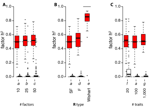
Figure 4: Latent factor heritabilities were accurately recovered. Distributions of factor $h^{2}$ estimates by simulation scenario. Each simulated factor was matched to the estimated factor with most similar trait-loadings as in Figure 5. Thin horizontal lines in each column show the simulated $h^{2}_{j}$ values. Each simulated factor was assigned $h^{2}=0.0$ (black) or $0.5$ (red), except in scenario e where all five factors were assigned $h^{2}=1$ (red). $h^{2}$ estimates are are grouped across all 10 simulations of each scenario. (A) Increasing numbers of simulated factors. (B) Different properties of the $\mathbf{R}$ matrix. (C) Different numbers of traits.

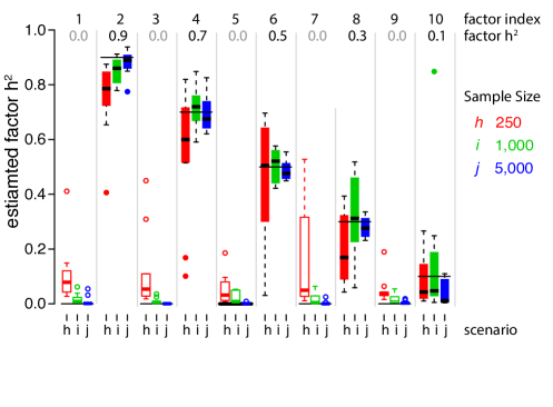
Figure 5: Latent factor heritabilities were accurately recovered. Distributions of factor $h^{2}$ estimates for scenarios h-j. These scenarios differed in the number of individuals sampled. 10 factors were generated in each simulation and assigned $h^{2}$s between 0.0 and 0.9. After fitting our factor model to each simulated dataset, the simulated factors were matched to estimated factors based on the trait-loading vector angles. Each boxplot shows the distribution of $h^{2}$ estimates for each simulated factor across 10 simulations. Note that the trait-loadings for each factor differed in each simulation; only the $h^{2}$ values remained the same. Thin horizontal lines in each column show the simulated $h^{2}_{j}$ values. Colors correspond to the scenario, and filled boxes/circles are used for factors with $h^{2}_{j}>0$.

Figure 6: Heritability estimates for each individual trait were accurate. The heritability of each individual trait was estimated as $h^{2}_{i}=\mathbf{G}_{ii}/\mathbf{P}_{ii}$. RMSE $=\sqrt{\frac{1}{p}\sum\limits_{i=1}^{p}(\hat{h}^{2}_{i}-h^{2}_{i})^{2}}$ was calculated for each simulation. Boxplots show the distribution of RMSE values for each scenario. A. Increasing numbers of simulated factors. B. Different properties of the $\mathbf{R}$ matrix. C. Different numbers of traits. D. Different numbers of sampled individuals.

3.2 Gene expression example:

Our estimate of the G-matrix from the Drosophila gene expression data was qualitatively similar to the original estimate (Figure 7B, and compare to Figure 7a in Ayroles et al. (2009)). Estimates of the broad-sense heritability of each gene were also similar ($r=0.74$). While a direct comparison of the dominant G-matrix subspace recovered by our model and the estimate by Ayroles et al. (2009) was not possible because individual covariances were not reported, we could compare the two estimates of the underlying structure. Using the Modulated Modularity Clustering (MMC) algorithm Stone and Ayroles (2009), Ayroles et al. (2009) identified 20 modules of genetically correlated transcripts post-hoc. Our model identified 27 latent factors (Figure 7D-F), of which 13 were large factors (explaining $>1\%$ variation in $2^{+}$ genes). The large factors were consistent ($r>0.95$) across three 3 parallel chains of the Gibbs sampler. Many factors were similar to the modules identified by MMC (Figure 7E). Some of the factors were nearly one-to-one matches to modules (e.g., factor 10 with module 8, and factor 14 with module 12). However, others merged together two or more modules (e.g., factor 1 with modules 7 and 9, and factor 2 with modules 4, 13, 16-20). And some entire modules were part of two or more factors (e.g., module 17 was included in factors 2 and 4, and module 18 was included in factors 2 and 16).

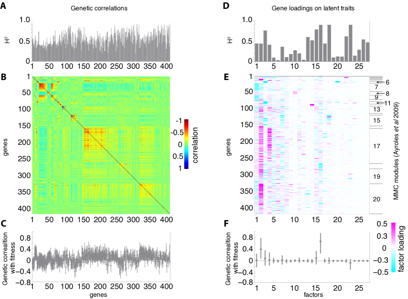
Figure 7: Among-line covariance of gene expression and competitive fitness in Drosophila is modular. A-C Genetic (among-line) architecture of 414 gene expression traits Ayroles et al. (2009). A. Posterior mean broad-sense heritabilities ($H^{2}$) for the 414 genes. B. Posterior mean genetic correlations among these genes. C. Posterior means and $95\%$ highest posterior density (HPD) intervals around estimates of genetic correlations between each gene and competitive fitness. For comparison, see Figure 7a of Ayroles et al. (2009). D-F. Latent trait structure of gene expression covariances. D Posterior mean $H^{2}$ for each estimated latent trait. E. Posterior mean gene loadings on each latent trait. F. Posterior means and $95\%$ (HPD) intervals around estimates of genetic correlations between each latent trait and competitive fitness. The right-axis of panel E. groups genes into modules inferred using Modulated Modularity Clustering Stone and Ayroles (2009); Ayroles et al. (2009).

Each factor (column of $\mathbf{\Lambda}$) represents a sparse set of genes that are highly correlated in their expression, possibly due to common regulation by some latent developmental trait. Using the Database for Annotation, Visualization and Integrated Discovery (DAVID) v6.7 Huang et al. (2009a, b), we identified several factors that were individually enriched (within this set of 414 genes) for defense and immunity, nervous system function, odorant binding, and transcription and cuticle formation. Similar molecular functions were identified among the modules identified by Ayroles et al. (2009). By inferring factors at the level of phenotypic variation, rather than the among-line covariances, we could directly estimate the broad-sense heritability ($H^{2}$) of these latent traits themselves. Figure 7D shows these $H^{2}$ estimates for each latent trait. Several of the factors have very low ($<0.2$) or very high ($>0.75$) $H^{2}$ values. Selection on the later latent traits would likely be considerably more efficient than the former.

Finally, by adding a competitive fitness as a 415th trait in the analysis, we could estimate the among-line correlation between the expression of each gene and this fitness-related trait (Figure 7C). Many (60/414 $\sim 15\%$ of all genes analyzed) of the $95\%$ highest posterior density (HPD) intervals on the among-line correlations did not included zero, although most of these correlations were low (for $85\%$ of genes, $|r|<0.25$) with a few as large as $|r|\sim 0.45$. More significantly, we could also estimate the genetic correlation between competitive fitness and each of the latent traits defined by the 27 factors (Figure 7F). Most factors had near-zero genetic correlations with competitive fitness. However, the genetic correlations between competitive fitness and factors 2 and 16 were large and highly significant, suggesting potentially interesting genetic relationships between these two latent traits and fitness.

4 Discussion

The Bayesian genetic sparse factor model performs well on both simulated and real data, and thus opens the possibility of incorporating high dimensional traits into evolutionary genetic studies and breeding programs. Technologies for high-dimensional phenotyping are becoming widely available in evolutionary biology and ecology so methods for modeling such traits are needed. Gene expression traits in particular provide a way to measure under-appreciated molecular and developmental traits that may be important for evolution, and technologies exist to measure these traits on very large scales. Our model can also be applied to other molecular traits (e.g., metabolites or protein concentrations), high dimensional morphological traits (e.g., outlines of surfaces from geometric morphometrics), or gene-environment interactions (e.g., the same trait measured in multiple environments).

4.1 Scalability of the method:

The key advantage of the Bayesian genetic sparse factor model over existing methods is its ability to provide robust estimates of covariance parameters for datasets with large numbers of traits. In this study, we demonstrated high performance of the model for $100-1,000$ simulated traits, and robust results on real data with 415. Similar factor models (without the genetic component) have been applied to gene expression datasets with thousands of traits Bhattacharya and Dunson (2011), and we expect the genetic model to perform similarly. The main limitation will be computational time, which scales roughly linearly with the number of traits analyzed (assuming the number of important factors grows more slowly). As an example, analyses of simulations from scenario g with 1,000 traits and 1,000 individual took about 4 hours to generate 12,000 posterior samples on a laptop computer with a 4-core 2.4 GHz Intel Core i7, while analyses of scenario a with 100 traits took about 45 minutes. Parallel computing techniques may speed up analyses in cases of very large (e.g., 10,000+) numbers of traits.

The main reason that our model scales well in this way is that under our prior, each factor is sparse. Experience with factor models in fields such as gene expression analysis, economics, finance, and social sciences Fan et al. (2011), as well as with genetic association studies (e.g., Engelhardt and Stephens 2010; Stegle et al. 2010; Parts et al. 2011) demonstrates that sparsity (or shrinkage) is necessary to perform robust inference on high-dimensional data Bickel and Levina (2008b, a); el Karoui (2008); Meyer and Kirkpatrick (2010). Otherwise, sampling variability can overwhelm any true signals, leading to unstable estimates. Here, we used the t-distribution as a shrinkage prior, following Bhattacharya and Dunson (2011), but many other choices are possible Armagan et al. (2011).

4.2 Applications to evolutionary quantitive genetics:

The G-matrix features prominently in the theory of evolutionary quantitative genetics, and its estimation has been a central goal of many experimental and observational studies Walsh and Blows (2009). Since our model is built on the standard “animal model” mixed effect model framework, it is flexible and can be applied to many experimental designs or studies. And since our model is Bayesian and naturally produces estimates within the parameter space, posterior samples from the Gibbs sampler provide convenient credible intervals for the G-matrix itself and many evolutionarily important parameters, such as trait-specific heritabilities or individual breeding values Sorensen and Gianola (2010).

An important use of G-matrices is to predict the response of a set of traits to selection Lande (1979). Applying Robertson’s 2nd theorem of natural selection, the response in $\mathbf{\bar{y}}$ will equal the additive genetic covariance between the vector of traits and fitness ($\Delta\mathbf{\bar{y}}=\sigma_{A}(\mathbf{y},\bar{w})$) Rausher (1992); Walsh and Blows (2009). This quantity can be estimated directly from our model if fitness is included as the $p^{*}=(p+1)$th trait:

$$\Delta\mathbf{\bar{y}}=\mathbf{\Lambda}_{u_{/p^{*}}}\mathbf{\Lambda}^{T}_{u_{p^{*}}},$$

where $\mathbf{\Lambda}_{u_{/p^{*}}}$ contains all rows of $\mathbf{\Lambda}_{u}$ except the row for fitness, and $\mathbf{\Lambda}_{u_{p^{*}}}$ contains only the row of $\mathbf{\Lambda}_{u}$ corresponding to fitness. Similarly, the quantity $1-\Psi_{u_{p^{*}}}/\mathbf{G}_{p^{*},p^{*}}$ equals the percentage of genetic variation in fitness accounted for by variation in the observed traits Walsh and Blows (2009), which is useful for identifying other traits that might be relevant for fitness.

On the other hand, our model is not well suited to estimating the dimensionality of the G-matrix. A low-rank G-matrix means that there are absolute genetic constraints on evolution Lande (1979). Several methods provide statistical tests for the rank of the G-matrix (e.g., Hine and Blows 2006; Kirkpatrick and Meyer 2004; Mezey and Houle 2005). We use a prior that shrinks the magnitudes of higher index factors to provide robust estimates of the largest factors. This will likely have a side-effect of underestimating the total number of factors, although this effect was not observed in our simulations. However, absolute constraints appear rare Houle (2010), and the dimensions of the G-matrix with the most variation are likely those with the greatest effect on evolution in natural populations Schluter (1996); Kirkpatrick (2009). Our model should estimate these dimensions well. From a practical standpoint, pre-selecting the number of factors has plagued other reduced-rank estimators of the G-matrix (e.g., Kirkpatrick and Meyer 2004; Hine and Blows 2006; Meyer 2009). Our prior is based on an infinite factor model Bhattacharya and Dunson (2011), and so no a priori decision is needed. Instead, the parameters of the prior distribution become important modeling decisions. In our experience, a relatively diffuse prior on $\delta_{l}$ with $a_{2}=3,b_{2}=1$ tends to work well.

4.3 Biological interpretation of factors:

Genetic modules are sets of traits likely to evolve together. By assuming that the developmental process is modular, we can model each latent trait as affecting a limited number of observed traits. A unique feature of our model is the fact that we estimate genetic and environmental factors jointly, instead of separately as in classic multilevel factor models (e.g., Goldstein 2010). If each factor represents a true latent trait (e.g., variation in a developmental process), it is reasonable to decompose variation in this trait into genetic and environmental components. We directly estimate the heritability of the traits underlying each factor, and therefore can use our model to predict the evolution of these latent traits.

Other techniques for identifying genetic modules have several limitations. The MMC algorithm Stone and Ayroles (2009); Ayroles et al. (2009) does not infer modules in an explicit quantitative genetic framework, and constraints each trait to belong to only one module. In some analyses (e.g., Mcgraw et al. 2011), each major eigenvector of the $\mathbf{G}$ or $\mathbf{P}$ matrices is treated as underlying module. These eigenvectors can be modeled directly (e.g., Kirkpatrick and Meyer 2004), but the biological interpretation of the eigenvectors is unclear because of the mathematical constraint that the they be orthogonal Hansen and Houle (2008). In classic factor models (such as proposed by Meyer (2009), or de Los Campos and Gianola (2007)), factors are not identifiable Meyer (2009), and so the identity of the underlying modules is unclear. Under our sparsity prior, factors are identifiable (up to a sign-flip: the loadings on each factor can be multiplied by $-1$ without affecting its probability under the model, but this does not change which traits are associated with each factor). In simulations and with the Drosophila gene expression data, independent MCMC chains consistently identify the same dominant factors. Therefore the observed traits associated with each factor can reliably be used to characterize the developmental process represented by the latent trait.

4.4 Extensions:

Our model is built on the classic mixed effect model common in quantitative genetics Henderson (1984). It is therefore straightforward to extend to models with additional fixed or random effects (e.g., dominance or epistatic effects) for each trait. However, the update equation for $h^{2}_{j}$ in the Gibbs sampler described in the Appendix does not allow additional random effects in the model for the latent factors themselves, although other formulations are possible. A second extension relates to the case when the relationship matrix among individuals ($\mathbf{A}$) is unknown. Here, relationship estimates from genotype data can be easily incorporated. As such, our model is related to a recently proposed sparse factor model for genetic associations with intermediate phenotypes Parts et al. (2011). These authors introduced prior information on genetic modules from gene function and pathway databases which could be incorporated in our model in a similar way.

5 Conclusions

The Bayesian genetic sparse factor model for genetic analysis that we propose provides a novel approach to genetic estimation with high-dimensional traits. We anticipate that incorporating many diverse phenotypes into genetic studies will provide powerful insights into evolutionary processes. The use of highly-informative but biologically grounded priors is necessary for making inferences on high-dimensional data, and can help identify developmental mechanisms underlying phenotypic variation in populations.

6 Appendix

6.1 Posterior sampling:

We estimate the posterior distribution of the Bayesian genetic sparse factor model with an adaptive Gibbs sampler based on the procedure proposed by Bhattacharya and Dunson (2011). The value $k^{*}$ at which columns in $\mathbf{\Lambda}$ are truncated is set using an adaptive procedure Bhattacharya and Dunson (2011). Given a truncation point, the sampler iterates through the following steps:

1. If missing observations are present, values are drawn independently from univariate normal distributions parameterized by the current values of all other parameters:

   $$\pi(y_{im}\mid-)\sim\mbox{N}\left(\mathbf{x}^{(j)}\mathbf{b}_{i}+\mathbf{f}^{(m)}\mathbf{\lambda}_{i}+\mathbf{z}^{(m)}\mathbf{\delta}_{i},(\sigma^{-2}_{i})^{-1}\right)$$

   where $y_{im}$ is the imputed phenotype value for the $i$-th trait in individual $m$. The three components of the mean are: $\mathbf{x}^{(m)}$ the row vector of fixed effect covariates for individual $m$ times $\mathbf{b}_{i}$, the $i$th column of the fixed effect coefficient matrix; $\mathbf{f}^{(m)}$, the row vector of factor scores on the $k^{*}$ factors for individual $m$ times $\mathbf{\lambda}_{i}$, the row of the factor loading matrix for trait $i$; and $\mathbf{z}^{(m)}$, the row vector of the random (genetic) effect incidence matrix for individual $m$ times $\mathbf{\delta}_{i}$, the vector of residual genetic effects for trait $i$ not accounted for by the $k^{*}$ factors. Finally, $\sigma^{-2}_{i}$ is the residual precision of trait $i$. All missing data can be drawn in a single block update.

2. The fixed effect coefficient matrix $\mathbf{B}$, the truncated factor loading matrix $\mathbf{\Lambda}_{k^{*}}$ and the residual genetic effects matrix $\mathbf{\Delta}$ can be stacked into a single matrix, and then its columns factor into independent multivariate normal conditional posteriors:

   $$\pi\left(\left[\begin{array}[]{c}\mathbf{b}_{i}\\ \mathbf{\delta}_{i}\\ \mathbf{\lambda}_{i}\\ \end{array}\right]\big{|}-\right) \sim\mbox{N}\left(\mathbf{C}^{-1}\mathbf{W}^{T}\sigma_{i}^{2}\mathbf{y}_{i},\mathbf{C}^{-1}\right),$$

   where $\mathbf{W}$ and $\mathbf{C}$ are defined as:

   $$\mathbf{W} =[\mathbf{X}\;\mathbf{Z}\;\mathbf{F}]$$

   $$\mathbf{C} =\left[\begin{array}[]{ccc}\mathbf{0}&\mathbf{0}&\mathbf{0}\\ \mathbf{0}&\psi_{a_{ii}}^{-2}\mathbf{A}^{-1}&\mathbf{0}\\ \mathbf{0}&\mathbf{0}&\mbox{Diag}(\phi_{ij}\tau_{j})\end{array}\right]+\sigma_{i}^{-2}\mathbf{W}\mathbf{W}^{T}.$$

3. The conditional posterior of the factor scores $\mathbf{F}$ is a matrix variate normal distribution:

   $$\pi\left(\mathbf{F}\mid-\right) \sim\mbox{MN}_{n,k^{*}}\left(\mathbf{C}^{-1}\left(\tilde{\mathbf{Y}}\mathbf{\Psi}_{e}^{-1}\mathbf{\Lambda_{k^{*}}}+\mathbf{Z}\mathbf{F}_{u}\mbox{Diag}(1-h^{2}_{i})^{-1}\right),\mathbf{C}^{-1}\right)$$

   where $\mathbf{C}$ is:

   $$\mathbf{C} =\mathbf{\Lambda}_{k^{*}}^{T}\mathbf{\Psi}_{e}^{-1}\mathbf{\Lambda}_{k^{*}}+\mbox{Diag}(1-h^{2}_{i})^{-1}$$

   and $\tilde{\mathbf{Y}}$ is:

   $$\tilde{\mathbf{Y}}=\mathbf{Y}-\mathbf{X}\mathbf{B}-\mathbf{Z}\mathbf{\Delta}.$$

4. The conditional posterior of the genetic effects on the factors, $\mathbf{F}_{u}$ factors into independent multivariate normals for each factor $\mathbf{f}_{u_{j}},j=1\dots k^{*}\mbox{ st }h^{2}_{j}\neq 0$:

   $$\pi\left(\mathbf{f}_{u_{j}}\mid-\right) \sim\mbox{MN}\left(\mathbf{C}^{-1}(1-h^{2}_{j})^{-1}\mathbf{Z}\mathbf{F}_{m},\mathbf{C}^{-1}\right)$$

   where $\mathbf{C}$ is:

   $$\mathbf{C} =(1-h^{2}_{j})^{-1}\mathbf{Z}\mathbf{Z}^{T}+(h^{2}_{j})^{-1}\mathbf{A}^{-1}.$$

5. The conditional posterior for each of the latent factor heritabilities $h^{2}_{j},j=1\dots k^{*}$ is calculated by integrating out $\mathbf{F}_{u}$ and summing over all possibilities of $h^{2}_{j}$, since the prior on this parameter is discrete:

   $$\pi\left(h^{2}_{j}=h^{2}\mid-\right) =\frac{\mbox{N}\left(\mathbf{F}_{j}\mid\mathbf{0},h^{2}\mathbf{Z}\mathbf{A}\mathbf{Z}^{T}+(1-h^{2})\mathbf{I}_{n}\right)\pi(h^{2}_{j}=h^{2})}{\sum\limits_{l=1}^{n_{h}}\mbox{N}\left(\mathbf{F}_{j}\mid\mathbf{0},h^{2}_{l}\mathbf{Z}\mathbf{A}\mathbf{Z}^{T}+(1-h^{2}_{l})\mathbf{I}_{n}\right)\pi(h^{2}_{j}=h^{2}_{l})}$$

   where $\mbox{N}(\mathbf{x}\mid\mathbf{\mu},\Sigma)$ is the multivariate normal density with mean $\mathbf{\mu}$ and variance $\Sigma$, evaluated at $\mathbf{x}$, $h^{2}_{l}=l/n_{h}$, and $\pi(h^{2}_{j}=h^{2})$ Is the prior probability that $h^{2}_{j}=h^{2}$. Given this conditional posterior, $h^{2}_{j}$ is sampled from a multinomial distribution.

6. The conditional posterior of the trait-factor loading variance $\phi_{ih}$ for trait $i$ on factor $h$ is:

   $$\pi(\phi_{ih}\mid-)\sim\mbox{Ga}\left(\frac{\nu+1}{2},\frac{\nu+\lambda_{ih}^{2}}{2}\right).$$

7. The conditional posterior of $\delta_{m},m=1\dots k^{*}$ is as follows. For $\delta_{1}$:

   $$\pi(\delta_{1}\mid-)\sim\mbox{Ga}\left(a_{1}+\frac{pk^{*}}{2},b_{1}+\frac{1}{2}\sum\limits_{l=1}^{k^{*}}\tau_{l}^{(1)}\sum\limits_{j=1}^{p}\phi_{jl}\lambda^{2}_{jl}\right)$$

   and for $\delta_{h},h\geq 2$:

   $$\pi(\delta_{h}\mid-)\sim\mbox{Ga}\left(a_{2}+\frac{p}{2}(k^{*}-h+1),b_{2}+\frac{1}{2}\sum\limits_{l=h}^{k^{*}}\tau_{l}^{(h)}\sum\limits_{j=1}^{p}\phi_{jl}\lambda^{2}_{jl}\right)$$

   where $\tau_{l}^{(h)}=\prod\limits_{t=1,t\neq h}^{l}\delta_{t}$ for $h=1\dots k^{*}$.

8. The conditional posteriors for the precision of the residual genetic effects of trait $i$, $\psi_{u_{ii}}$, is:

   $$\pi(\psi_{u_{ii}}\mid-)\sim\mbox{Ga}\left(a_{g}+\frac{r}{2},b_{g}+\frac{1}{2}\mathbf{\delta}_{i}^{T}\mathbf{\delta}_{i}\right).$$

9. The conditional posteriors for the model residuals of trait $i$, $\sigma_{i}^{-2}$, is:

   $$\pi(\sigma_{i}^{-2}\mid-)\sim\mbox{Ga}\left(a_{r}+\frac{n}{2},b_{r}+\frac{1}{2}\sum\limits_{j=1}^{n}\left(y_{ij}-\mathbf{x}^{(j)}\mathbf{b}_{i}-\mathbf{f}^{(j)}\mathbf{\lambda}_{i}-\mathbf{z}^{(j)}\mathbf{\delta}_{i}\right)^{2}\right).$$

Other random effects, such as the line $\times$ sex effects modeled in the gene expression example of this paper can be incorporated into this sampling scheme in much the same way as the residual genetic effects, $\mathbf{\Delta}$, are included here.

7 Acknowledgments

We would like to thank Barbara Engelhardt, Iulian Pruteanu-Malinici, Jenny Tung, and two anonymous reviewers for comments and advice on this method.

References

- Armagan et al. (2011) Armagan, A., D. B. Dunson, and M. Clyde, 2011 Generalized Beta Mixtures of Gaussians. Neural Information Processing Systems: arXiv:1107.4976.
- Ayroles et al. (2009) Ayroles, J. F., M. A. Carbone, E. A. Stone, K. W. Jordan, R. F. Lyman, M. M. Magwire, S. M. Rollmann, L. H. Duncan, F. Lawrence, R. R. H. Anholt, and T. F. C. Mackay, 2009 Systems genetics of complex traits in Drosophila melanogaster. Nat Genet 41(3): 299–307.
- Bhattacharya and Dunson (2011) Bhattacharya, A. and D. B. Dunson, 2011 Sparse Bayesian infinite factor models. Biometrika 98(2): 291–306.
- Bickel and Levina (2008a) Bickel, P. J. and E. Levina, 2008a Covariance regularization by thresholding. Annals of Statistics 36: 2577–2604.
- Bickel and Levina (2008b) Bickel, P. J. and E. Levina, 2008b Regularized estimation of large covariance matrices. Annals of Statistics 36: 199–227.
- Blows et al. (2004) Blows, M. W., S. F. Chenoweth, and E. Hine, 2004 Orientation of the genetic variance-covariance matrix and the fitness surface for multiple male sexually selected traits. The American Naturalist 163(3): 329–340.
- Cantor et al. (2010) Cantor, R. M., K. Lange, and J. S. Sinsheimer, 2010 Prioritizing GWAS Results: A Review of Statistical Methods and Recommendations for Their Application. Am J Hum Genet 86(1): 6–22.
- Carvalho et al. (2008) Carvalho, C. M., J. Chang, J. E. Lucas, J. R. Nevins, Q. Wang, and M. West, 2008 High-Dimensional Sparse Factor Modeling: Applications in Gene Expression Genomics. Journal of the American Statistical Association 103(484): 1438–1456.
- Cheverud (1996) Cheverud, J. M., 1996 Developmental Integration and the Evolution of Pleiotropy. Integrative and Comparative Biology 36(1): 44–50.
- Davidson and Levine (2008) Davidson, E. and M. Levine, 2008 Properties of developmental gene regulatory networks. Proc Natl Acad Sci USA 105(51): 20063–20066.
- Dawid (1981) Dawid, A. P., 1981 Some matrix-variate distribution theory: Notational considerations and a Bayesian application. Biometrika 68(1): 265–274.
- de la Cruz et al. (2010) de la Cruz, O., X. Wen, B. Ke, M. Song, and D. L. Nicolae, 2010 Gene, region and pathway level analyses in whole-genome studies. Genet Epidemiol 34: 222–231.
- de Los Campos and Gianola (2007) de Los Campos, G. and D. Gianola, 2007 Factor analysis models for structuring covariance matrices of additive genetic effects: a Bayesian implementation. Genet Sel Evol 39(5): 481–494.
- el Karoui (2008) el Karoui, N., 2008 Operator norm consistent estimation of large dimensional sparse covariance matrices. Annals of Statistics 36: 2717–2756.
- Engelhardt and Stephens (2010) Engelhardt, B. E. and M. Stephens, 2010 Analysis of Population Structure: A Unifying Framework and Novel Methods Based on Sparse Factor Analysis. PLoS Genet 6(9): e1001117.
- Fan et al. (2011) Fan, J., J. Lv, and L. Qi, 2011 Sparse High Dimensional Models in Economics. Annu Rev Econom 3: 291–317.
- G R Knight (1957) G R Knight, A. R., 1957 Fitness as a Measurable Character in Drosophila. Genetics 42(4): 524.
- Gelman (2006) Gelman, A., 2006 Prior distributions for variance parameters in hierarchical models . Bayesian Analysis 1(3): 515–533.
- Gibson and Weir (2005) Gibson, G. and B. Weir, 2005 The quantitative genetics of transcription. Trends Genet 21(11): 616–623.
- Goldstein (2010) Goldstein, H., 2010 Multilevel Factor Analysis, Structural Equation and Mixture Models, pp. 189–200. John Wiley & Sons, Ltd.
- Hahn et al. (2013) Hahn, P. R., C. M. Carvalho, and S. Mukherjee, 2013 Partial Factor Regression. Journal of the American Statistical Association.
- Hansen and Houle (2008) Hansen, T. F. and D. Houle, 2008 Measuring and comparing evolvability and constraint in multivariate characters. J Evol Biol 21(5): 1201–1219.
- Hartl and Jungen (1979) Hartl, D. L. and H. Jungen, 1979 Estimation of Average Fitness of Populations of Drosophila melanogaster and the Evolution of Fitness in Experimental Populations. Evolution 33(1): 371–380.
- Hastie et al. (2003) Hastie, T., R. Tibshirani, and J. H. Friedman, 2003 The Elements of Statistical Learning. Springer.
- Hayes and Hill (1981) Hayes, J. F. and W. G. Hill, 1981 Modification of estimates of parameters in the construction of genetic selection indices (’bending’). Biometrics 37(3): 483–493.
- Henderson (1984) Henderson, C. R., 1984 Applications of linear models in animal breeding. Guelph, Ca: University of Guelph.
- Hine and Blows (2006) Hine, E. and M. W. Blows, 2006 Determining the effective dimensionality of the genetic variance-covariance matrix. Genetics 173(2): 1135–1144.
- Houle (2010) Houle, D., 2010 Colloquium papers: Numbering the hairs on our heads: the shared challenge and promise of phenomics. Proc. Natl. Acad. Sci. U.S.A. 107 Suppl 1: 1793–1799.
- Huang et al. (2009a) Huang, D. W., B. T. Sherman, and R. A. Lempicki, 2009a Bioinformatics enrichment tools: paths toward the comprehensive functional analysis of large gene lists. Nucl. Acids Res. 37(1): 1–13.
- Huang et al. (2009b) Huang, D. W., B. T. Sherman, and R. A. Lempicki, 2009b Systematic and integrative analysis of large gene lists using DAVID bioinformatics resources. Nat Protoc 4(1): 44–57.
- Jaffrezic et al. (2002) Jaffrezic, F., M. S. White, R. Thompson, and P. M. Visscher, 2002 Contrasting Models for Lactation Curve Analysis. Journal of Dairy Science 85: 968–975.
- Kirkpatrick (2009) Kirkpatrick, M., 2009 Patterns of quantitative genetic variation in multiple dimensions. Genetica 136(2): 271–284.
- Kirkpatrick and Heckman (1989) Kirkpatrick, M. and N. Heckman, 1989 A quantitative genetic model for growth, shape, reaction norms, and other infinite-dimensional characters. J Math Biol 27(4): 429–450.
- Kirkpatrick and Meyer (2004) Kirkpatrick, M. and K. Meyer, 2004 Direct estimation of genetic principal components: Simplified analysis of complex phenotypes. Genetics 168(4): 2295–2306.
- Kruuk (2004) Kruuk, L. E. B., 2004 Estimating genetic parameters in natural populations using the ’animal model’. Philos T Roy Soc B 359(1446): 873–890.
- Krzanowski (1979) Krzanowski, W. J., 1979 Between-Groups Comparison of Principal Components. J Am Stat Assoc 74(367): 703–707.
- Lande (1979) Lande, R., 1979 QUANTITATIVE GENETIC-ANALYSIS OF MULTIVARIATE EVOLUTION, APPLIED TO BRAIN - BODY SIZE ALLOMETRY. Evolution 33(1): 402–416.
- Lucas et al. (2006) Lucas, J., C. Carvalho, Q. Wang, A. Bild, J. Nevins, and M. West, 2006 Sparse statistical modelling in gene expression genomics. Bayesian Inference for Gene Expression and Proteomics 1.
- Lynch and Walsh (1998) Lynch, M. and B. Walsh, 1998 Genetics and analysis of quantitative traits (1 ed.). Sinauer Associates Inc.
- Mcgraw et al. (2011) Mcgraw, E. A., Y. H. Ye, B. Foley, S. F. Chenoweth, M. Higgie, E. Hine, and M. W. Blows, 2011 HIGH-DIMENSIONAL VARIANCE PARTITIONING REVEALS THE MODULAR GENETIC BASIS OF ADAPTIVE DIVERGENCE IN GENE EXPRESSION DURING REPRODUCTIVE CHARACTER DISPLACEMENT. Evolution 65(11): 3126–3137.
- Meyer (2005) Meyer, K., 2005 Advances in methodology for random regression analyses. Australian journal of Experimental Agriculture 45: 847–858.
- Meyer (2009) Meyer, K., 2009 Factor-analytic models for genotype x environment type problems and structured covariance matrices. Genet Sel Evol 41: 21.
- Meyer and Kirkpatrick (2007) Meyer, K. and M. Kirkpatrick, 2007 A NOTE ON BIAS IN REDUCED RANK ESTIMATES OF COVARIANCE MATRICES. Proc. Ass. Advan. Anim. Breed. Genet 17: 154–157.
- Meyer and Kirkpatrick (2008) Meyer, K. and M. Kirkpatrick, 2008 Perils of Parsimony: Properties of Reduced-Rank Estimates of Genetic Covariance Matrices. Genetics 180: 1153–1166.
- Meyer and Kirkpatrick (2010) Meyer, K. and M. Kirkpatrick, 2010 Better estimates of genetic covariance matrices by ”bending” using penalized maximum likelihood. Genetics 185(3): 1097–1110.
- Mezey and Houle (2005) Mezey, J. and D. Houle, 2005 The dimensionality of genetic variation for wing shape in Drosophila melanogaster. Evolution 59(5): 1027–1038.
- Neal (1996) Neal, R. M., 1996 Bayesian Learning for Neural Networks. Secaucus, NJ, USA: Springer-Verlag New York, Inc.
- Parts et al. (2011) Parts, L., O. Stegle, J. Winn, and R. Durbin, 2011 Joint genetic analysis of gene expression data with inferred cellular phenotypes. PLoS Genet 7(1): e1001276.
- Pletcher and Geyer (1999) Pletcher, S. D. and C. J. Geyer, 1999 The genetic analysis of age-dependent traits: modeling the character process. Genetics 153(2): 825–835.
- Poggio and Smale (2003) Poggio, T. and S. Smale, 2003 The Mathematics of Learning: Dealing with Data. Notices of the American Mathematical Society 50: 2003.
- Rausher (1992) Rausher, M. D., 1992 THE MEASUREMENT OF SELECTION ON QUANTITATIVE TRAITS - BIASES DUE TO ENVIRONMENTAL COVARIANCES BETWEEN TRAITS AND FITNESS. Evolution 46(3): 616–626.
- Schluter (1996) Schluter, D., 1996 Adaptive radiation along genetic lines of least resistance. Evolution 50(5): 1766–1774.
- Sorensen and Gianola (2010) Sorensen, D. and D. Gianola, 2010 Likelihood, Bayesian and MCMC Methods in Quantitative Genetics (Statistics for Biology and Health). Springer.
- Stegle et al. (2010) Stegle, O., L. Parts, R. Durbin, and J. Winn, 2010 A Bayesian framework to account for complex non-genetic factors in gene expression levels greatly increases power in eQTL studies. PLoS Comput Biol 6(5): e1000770.
- Stone and Ayroles (2009) Stone, E. A. and J. F. Ayroles, 2009 Modulated modularity clustering as an exploratory tool for functional genomic inference. PLoS Genet 5(5): e1000479.
- Tipping (2001) Tipping, M. E., 2001 Sparse bayesian learning and the relevance vector machine. J. Mach. Learn. Res. 1: 211–244.
- Wagner and Altenberg (1996) Wagner, G. and L. Altenberg, 1996 Perspective: Complex Adaptations and the Evolution of Evolvability. EVOLUTION-LAWRENCE KANSAS- 50: 967–976.
- Walsh and Blows (2009) Walsh, B. and M. W. Blows, 2009 Abundant Genetic Variation plus Strong Selection = Multivariate Genetic Constraints: A Geometric View of Adaptation. Annu Rev Ecol Evol S 40: 41–59.
- West (2003) West, M., 2003 Bayesian Factor Regression Models in the ”Large p, Small n” Paradigm. In Bayesian Statistics, pp. 723–732. Oxford University Press.
- Xiong et al. (2012) Xiong, Q., N. Ancona, E. R. Hauser, S. Mukherjee, and T. S. Furey, 2012 Integrating genetic and gene expression evidence into genome-wide association analysis of gene sets. Genome Research 22: 386–397.
- Zhou and Stephens (2012) Zhou, X. and M. Stephens, 2012 Genome-wide efficient mixed-model analysis for association studies. Nature Genetics 44: 821–824.