Bold Diagrammatic Monte Carlo technique for frustrated spin systems

Abstract

Using fermionic representation of spin degrees of freedom within the Popov-Fedotov approach we develop an algorithm for Monte Carlo sampling of skeleton Feynman diagrams for Heisenberg type models. Our scheme works without modifications for any dimension of space, lattice geometry, and interaction range, i.e. it is suitable for dealing with frustrated magnetic systems at finite temperature. As a practical application we compute uniform magnetic susceptibility of the antiferromagnetic Heisenberg model on the triangular lattice and compare our results with the best available high-temperature expansions. We also report results for the momentum-dependence of the static magnetic susceptibility throughout the Brillouin zone.

I Introduction

Properties of geometrically frustrated spin systems in various dimensions, geometries, and temperature regimes are at the heart of modern condensed matter physics. Here, frustration is a technical term which refers to the presence of competing forces that cannot be simultaneously satisfied. In numerous quantum antiferromagnets frustration often has a simple geometric origin. Localized spins on two- and three-dimensional lattices with triangular motifs, such as planar triangular antiferromagnet and three-dimensional pyrochlore antiferromagnets, cannot assume energetically favorable antiparallel orientation. Of three spins forming a minimal triangle, and interacting via simple antiferromagnetic pair-wise exchange interaction, only two can be made antiparallel, leaving the third one frustrated. In case of classical Ising spins, which can point up or down with respect to some axis, this leads to an extensive ground-state degeneracy: for example, in a system of $N$ Ising spins on a triangular lattice there are $\Omega_{N}=e^{0.323N}$ configurations having the same (minimal) energy. On a three-dimensional pyrochlore lattice of site-sharing tetrahedra, the (effectively) Ising spins of Dy₂Ti₂O₇, Ho₂Ti₂O₇ and Ho₂Sn₂O₇ realize Harris et al. (1997) fascinating spin ice physics Bramwell and Gingras (2001) where strong local ice rules (for any given tetrahedron, two of its spins must point in, and the other two - out) enforce long-ranged power-law correlations between spins Isakov et al. (2004), in effect realizing artificial magnetic field and fractionally charged magnetic monopoles Castelnovo et al. (2008)!

Quantum spins can exploit this extensive degeneracy via quantum-mechanical coupling between different configurations – their wave function can be thought of as a linear superposition of all degenerate microstates represented by classical patterns of up- and down-spins. In the case of strong coupling we may arrive at a quantum spin liquid (QSL) Pomeranchuk (1941); Balents (2010) state in which spins never settle in one particular configuration and continue their exploration forever. It is clear that such a state encodes highly nontrivial correlations between different spins when flipping of one spin induces that of its neighbors so that as a whole the spin system remains in the lowest-energy manifold. Extensive experimental Hiroi et al. (2001); Shimizu et al. (2003); Okamoto et al. (2007); Itou et al. (2007, 2008); Olariu et al. (2008); Yoshida et al. (2009); Okamoto et al. (2009); Mendels and Bert (2010); Nakatsuji et al. (2010); Vachon et al. (2011); Quilliam et al. (2011); Yamashita et al. (2012); Yan et al. (2012) and theoretical Anderson (1987); Wen (2002); Kitaev (2006); Meng et al. (2010); Varney et al. (2011); Dang et al. (2011); Yan et al. (2011); Isakov et al. (2011); Okumura et al. (2010); Yao and Kivelson (2012) search for materials and models which may realize this intriguing QSL state constitutes one of the main topics of the quantum spin physics. Currently there are several intensely researched materials that hold promise of realizing the elusive spin liquid state. Among them, we mention two-dimensional spin-1/2 organic triangular antiferromagnets EtMe₃Sb[Pd(dmit)₂]₂ Itou et al. (2007, 2008); Yamashita et al. (2012) and $\kappa$-(BEDT-TTF)₂Cu₂(CN)₃ Shimizu et al. (2003); Yamashita et al. (2012), spin-1 material NiGa₂S₄ Nakatsuji et al. (2010), a series of inorganic quasi-two-dimensional kagomé lattice antiferromagnets: herbersmithite ZnCu₃(OH)₆Cl₂ Olariu et al. (2008); Mendels and Bert (2010), volborthite Cu₃V₂O₇(OH)${}_{2}\cdot$2H₂O Hiroi et al. (2001); Yoshida et al. (2009), and vesignieite BaCu₃V₂O₈(OH)₂ Okamoto et al. (2009); Quilliam et al. (2011), and a three-dimensional hyperkagomé antiferromagnet Na₄Ir₃O₈ Okamoto et al. (2007).

Taking the system of frustrated spins to a finite temperature, where all experiments are done, adds thermal randomness to the picture. At a finite temperature $T$ even classical spins can explore different microstates from the lowest-energy manifold. This too leads to a strongly correlated (although not necessarily phase-coherent, as in the case of quantum spins at $T=0$) motion of spins which is often described by a term “cooperative paramagnet”. Even if the ground state of spin system is not a true spin liquid, but instead is one of the many possible ordered states, the spins will (thermally) disorder at sufficiently high temperature, $T\geq T_{0}$, where $T_{0}$ stands for the ordering temperature. In the usual, non-frustrated magnets the ordering temperature is determined by the exchange interaction energy $J$ and coordination number of the lattice $z$, $T_{0}\sim zS(S+1)J$. Quite generally, it is of the order of the Curie-Weiss temperature $\theta_{\rm cw}$ which is easily determined experimentally via high-temperature behavior of the spin susceptibility $\chi\propto(T-\theta_{\rm cw})^{-1}$. In antiferromagnets $\theta_{\rm cw}$ is negative, and, in the absence of frustration, its absolute value sets the scale at which correlations between spins become pronounced. Thus, $T_{0}\sim|\theta_{\rm cw}|$. Frustrated magnets are very different as there $T_{0}\ll|\theta_{\rm cw}|$ : despite experiencing strong interactions with each other, the spins can not “agree” on one particular pattern which would satisfy them all. In the case of a true spin liquid $T_{0}=0$ and the order never arrives. In the majority of studied situations the order does take place, $T_{0}>0$, but only at a temperature much lower than the naïve estimate provided by $|\theta_{\rm cw}|$. This results in a wide temperature interval $T_{0}<T<|\theta_{\rm cw}|$ where the spins are strongly interacting but remain in a disordered cooperative paramagnet state. In fact, the existence of such temperature (and energy) window represents a defining feature of the frustrated magnet, as argued by Ramirez Ramirez (1994) who introduced the frustration parameter $f=|\theta_{\rm cw}|/T_{0}$ (it is not uncommon to find a situation with $f\sim 100$ or greater).

Strong suppression of the ordering temperature can be also the consequence of close proximity to the quantum critical point, separating the spin-disordered state (such as a putative QSL) from the more usual ordered one. It is well established now Sachdev (1999) that the finite-temperature region above the quantum critical point, known as the quantum-critical region, is as informative of the quantum state of the many-body system as the unreachable $T=0$ ground state. The quantum-critical scaling of, say, the dynamic spin susceptibility contains information on the spin correlation length, dynamic exponent $z$ and other critical exponents characterizing spin systems of different symmetries and dimensions.

Importantly, there is a large number of high-precision probes—neutron and X-ray scattering, nuclear magnetic resonance, muon spin rotation, susceptibility, magnetization and specific heat measurements—which allow us to address various aspects of strange and conflicting behavior of frustrated quantum magnets experimentally in a wide range of energies and temperatures. Given that in many important cases the correlated spin-liquid region $T_{0}<T<|\theta_{\rm cw}|$ occupies most of the experimentally accessible temperature interval, unbiased understanding of correlations and dynamics in this regime becomes the major theoretical task.

Theoretical understanding of frustrated magnetism at finite temperature is severely limited by the lack of natural small parameter(s). As a result, possible analytical approaches require one to study suitably ‘deformed’ models, such as, for example, very popular and well developed large-component (large-$N$) version of the Heisenberg spin model on frustrated lattices. The small parameter is then provided by $1/N$, expansion in powers of which (about the $N=\infty$ limit) controls the calculation. However the physical limit of $S=1/2$ SU(2) lattice spins corresponds to rather small $N$: $3$ in the case of $O(N)$ generalization and $1$ in the case of $Sp(N)$. Whether or not continuation of the results from $N=\infty$ to the physical value is reliable remains an open (and case sensitive) question. Other popular ‘deformations’ include SU(2)-to-U(1) symmetry reduction(s) and quantum dimer model approaches. While very insightful and interesting in their own, applicability of these ‘modifications’ to the original problem is always an issue. While analytical approaches are extremely useful in providing us with qualitative physical insights and understanding, in frustrated magnets they often fall short of quantitative description desired by experimentalists. Numerical approaches are limited as well. Exact diagonalizations are restricted to small systems (about $40$ sites at most) due to the exponentially large Hilbert space while standard quantum Monte Carlo techniques usually suffer from the infamous ‘sign problem’. Powerful series expansion methods often start to diverge in the most interesting regime $T_{0}<T<|\theta_{\rm cw}|$. Variational tensor-network type methods are also suffering from finite-size limitations and are mostly limited to ground state properties.

In this article we combine the most versatile theoretical tool, Feynman diagrammatics, with the power of Monte Carlo sampling of complex configuration spaces. The simplest way of arriving at the diagrammatic technique for spins is to represent them by auxiliary fermions with imaginary chemical potential. This trick was introduced by Popov and Fedotov for spin-1/2 systems in Ref. Popov and Fedotov, 1988; *PopovFedotov2. The ultimate strength of the diagrammatic approach as compared, e.g. with high-temperature or strong coupling expansions, comes from its self-consistent (skeleton) formulation with automatic summation of certain classes of graphs up to infinite order. This lead to better convergence properties and the possibility of obtaining reliable results in the strong coupling regime. It turns out that skeleton formulations can be easily implemented within the sampling protocols leading to the so-called Bold Diagrammatic Monte Carlo (BDMC) Prokof’ev and Svistunov (2007) which obtains physical answers by computing contributions from millions of graphs and extrapolates them to the infinite diagram order. Recently, this method was successfully applied to the normal state of the Fermi-Hubbard model at moderate interaction strength Kozik et al. (2010) and the strongly correlated system of unitary fermions (the so-called BCS-BEC crossover problem) Van Houcke et al. (2012). It was, however, never implemented for models of quantum magnetism, which, at least at the formal level, can be also viewed as a fermionic system with strong correlations. Here we present the first attempt to achieve an accurate theoretical description of the correlated paramagnetic regime within the BDMC framework.

In what follows in Sec. II we consider a spin-1/2 Heisenberg type model at finite temperature and its auxiliary fermion version which admits the standard diagrammatic expansion. In Sec. III we formulate principles of the BDMC technique and the specific self-consistent scheme for dealing with skeleton diagrams based on fully dressed lines. We proceed with detailed description of the worm algorithm for efficient sampling of the resulting configuration space (updates, counters, and data processing) in Sec. IV. Our results for the triangular lattice antiferromagnet are presented, discussed, and compared to the best available finite temperature simulations based on numerical linked-cluster (NLC) expansions Rigol et al. (2007) and extrapolations of high-temperature series  Zheng et al. (2005) in Sec. V. We conclude with broader implications of this work and further developments in Sec. VI.

II Model and its ‘bold-line’ diagrammatic expansion

Consider the standard Heisenberg model

$$H=\sum_{i,j}J_{ij}\,{\vec{S}}_{i}\cdot{\vec{S}}_{j}\,,$$ (1)

where ${\vec{S}}$ are quantum spin-1/2 operators. The dimension of space, lattice geometry, and interaction range are assumed to be arbitrary. Now, the idea is to replace spin degrees of freedom with fermionic ones:

$${\vec{S}}_{i}\to\frac{1}{2}\sum_{\alpha,\beta}f_{i\alpha}^{\dagger}\vec{\sigma}_{\alpha\beta}f_{i\beta}^{\,}\,.$$ (2)

Here $f_{i\beta}$ is the second quantized operator annihilating a fermion with spin projection $\beta=\pm 1$ on site $i$, and $\vec{\sigma}$ are the Pauli matrices. As a result, we convert coupling between spins into the standard two-body interaction term $J_{ij,\alpha\beta\gamma\delta}\,f_{i\alpha}^{\dagger}f_{i\beta}^{\,}f_{j\gamma}^{\dagger}f_{j\delta}^{\,}$ with matrix element $J_{ij,\alpha\beta\gamma\delta}=(1/4)J_{ij}\vec{\sigma}_{\alpha\beta}\cdot\vec{\sigma}_{\gamma\delta}$. By doing so we also increase the Hilbert space on every site from 2 to 4 by adding non-physical states with zero and two fermions.

The benefit of the auxiliary fermion representation does not require explanation: once the spin model is mapped onto a familiar problem of interacting fermions one can employ numerous diagrammatic tricks to solve it. However, this raises an issue of eliminating contributions from unphysical states to the answer in a manner consistent with the diagrammatic technique. Remarkably, there is a very simple way to achieve the goal by adding the chemical potential term to the fermionic Hamiltonian Popov and Fedotov (1988); *PopovFedotov2 (see also Ref. Prokof’ev and Svistunov, 2011)

$$H_{F}=\sum_{ij,\alpha\beta\gamma\delta}J_{ij,\alpha\beta\gamma\delta}\,f_{i\alpha}^{\dagger}f_{i\beta}^{\,}f_{j\gamma}^{\dagger}f_{j\delta}^{\,}-\mu\sum_{i}(n_{i}-1)\,,$$ (3)

with complex $\mu=-i\pi T/2$ and $n_{i}=\sum_{\alpha}f_{i\alpha}^{\dagger}f_{i\alpha}^{\,}$. The added term commutes with the original Hamiltonian and has no effect on properties of the physical subspace $\{n_{i}=1\}$ whatsoever. Moreover, the grand canonical partition functions and spin-spin correlation functions of the original spin model and its fermionic version are also identical because (i) physical and non-physical sites decouple in the trace and (ii) the trace over non-physical states yields identical zero on every site. As a result, we arrive at a rather standard Hamiltonian for fermions interacting through two-body terms. Complex value of the chemical potential is essentially a zero price to pay for the luxury of having the diagrammatic technique.

Formally, the entire setup is similar to the fractional quantum Hall effect system because the non-interacting part of Eq. (3) describes particles with zero dispersion relation, i.e. we start building the solution from the degenerate manifold. There is one important difference though: in conventional fermionic systems both the Green’s function and the spin-spin (or density-density) correlation function contain direct physical information about the system. In spin systems the Green’s function is rather an auxiliary object which always remains localized on a single site. This does not imply any pathological behavior yet since the physical degrees of freedom are spins, i.e. bilinear combinations of fermionic operators. Correspondingly, the main object of interest is not the Green’s function of the system but the spin-spin correlation function, or magnetic susceptibility:

$$\chi(i,j,\tau)=\langle T_{\tau}S^{z}_{i}(0)S^{z}_{j}(\tau)\rangle=\frac{1}{3}\langle T_{\tau}{\vec{S}}_{i}(0)\cdot{\vec{S}}_{j}(\tau)\rangle\,,$$ (4)

where $T_{\tau}$ stands for the imaginary time ordering operator.

To simplify the presentation below we consider lattices with one atom per unit cell and make use of the lattice translation invariance; otherwise one would need to keep an index enumerating different sites in the unit cell. For the same reason we do not place the system into the external magnetic field to preserve the symmetry between up- and down-spins; in the presence of the magnetic field $H_{0}$ one has to add spin-dependent real part to the chemical potential $\mu\to\mu_{\alpha}=-i\pi T/2-\alpha H_{0}$ and take proper care of the spin index.

The diagrammatic technique itself for Eq. (3) is absolutely standard Fetter and Walecka (1971). The perturbative diagrams are expressed in terms of the non-interacting, or ’bare’, Green’s functions (particle propagators), $G^{(0)}_{\alpha\beta}(i,\tau)\equiv\delta_{i,0}\delta_{\alpha,\beta}G^{(0)}(\tau)$, and two-body interaction lines $J_{i-j,\alpha\beta\gamma\delta}$. The non-interacting Green’s function on a lattice in the imaginary time representation reads (below the Boltzmann constant $k_{B}=1$)

$$G^{(0)}(\tau>0)=-\,\frac{e^{\mu\tau}}{1+\exp(\mu/T)}=\frac{e^{\mu\tau}}{i-1}\,,$$ (5)

with conventional anti-periodic boundary conditions $G^{(0)}(\tau<0)=-G^{(0)}(1/T+\tau)$. In what follows we completely suppress the site index for purely local quantities. For the Heisenberg model the dependence of the interaction line on spin indexes is rather simple

$$J_{i-j,\alpha\beta\gamma\delta} = \frac{J_{i-j}}{4}\,\hat{M}_{\alpha\beta\gamma\delta}\,,$$

$$\hat{M}_{\alpha\beta\gamma\delta} = \alpha\gamma\,\delta_{\alpha,\beta}\delta_{\gamma,\delta}+2\,\delta_{\delta,\alpha}\delta_{\gamma,-\alpha}\delta_{\beta,-\alpha}\,,$$ (6)

The first term describes diagonal coupling between the spin densities on sites $i$ and $j$, while the second spin-flip term exchanges spin values, see Fig. 1. The magnitude of the spin-flip process is fixed by the SU(2) symmetry of the problem. Even when interactions are screened by many-body effects, see below, the retarded interaction has exactly the same dependence on spin indexes. An arbitrary perturbative diagram of order $n$ contributing to, say, the free-energy is obtained by (i) placing graphical elements depicted in Fig. 1 with some space/time variables $i$, $j$, and $\tau\in(0,1/T)$ and connecting incoming and outgoing propagators with the same spin and site index to each other in such a way that all points in the resulting graph are connected by some path.

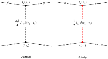
Figure 1: (Color online) Graphic representation of allowed interaction processes for the Heisenberg model.

III Bold Diagrammatic Monte Carlo scheme

The unique feature of diagrammatic expansions for propagators is that there are no numerical coefficients in the diagram weight depending on the diagram order or structure (this is not true for other well-known series such as virial, high-temperature, linked-cluster, strong-coupling, etc. expansions). This leads to the diagrammatic technique when certain infinite sets of diagrams, e.g. in the form of geometric series, are easily dealt with by algebraic means or reduced to self-consistently defined integral equations.

In the skeleton technique, the diagrams are classified according to some rule which eliminates the need for computing repeated blocks of diagrams. In the simplest scheme which is used in this paper, one identifies the proper self-energy blocks which consist of diagrams where all vertexes (points where two particle propagators and the interaction line meet) remain connected by some path when one removes any two lines of the same kind: two propagator lines with the same spin index or two interaction lines. We will refer to this set of diagrams as irreducible. The omitted diagrams are fully accounted for by replacing bare propagators and interaction lines in the proper self-energy blocks with exact propagators, $G(\tau)$, and screened interactions, $W(r,\tau)\hat{M}$. The resulting formulation is self-consistent and highly non-linear since $G$ and $W$ depend on proper self-energies through the Dyson type equations. If $\Sigma$ is the proper self-energy for the particle propagator, and $\Pi$ is an analogous quantity for the interaction line (better known as polarization operator) then (in Fourier representation $(r,\tau)\to(q,\omega_{m})$ for space-time variables)

$$G(m)=\frac{G^{(0)}(m)}{1-G^{(0)}(m)\Sigma(m)}\,,$$

$$W(q,m)=\frac{J(q)}{4-J(q)\Pi(q,m)}\equiv\frac{J(q)}{4}+\tilde{W}(q,m)\,.$$ (7)

where $J(q)=\sum_{r}e^{iqr}J(r)$. Due to fermionic/bosonic nature of propagators $G$/$W$ we have different definitions of the Matsubara frequency here, $\omega_{m}=2\pi T(m+1/2)$ for $(G,\Sigma)$ and $\omega_{m}=2\pi Tm$ for $(W,\Pi)$. Note also that we split the $W$ function into two parts by separating out the original coupling. This is done for technical reasons explained below; here we simply point out that in the imaginary time domain this is equivalent to paying special attention to the $\delta$-functional contribution, $W(q,\tau)=\tfrac{1}{4}J(q)\,\delta(\tau)+\tilde{W}(q,\tau)$. Correspondingly, for graphical representation of the diagrams we use wavy lines for $\tilde{W}$ and dashed vertical lines for bare coupling. The corresponding (rather standard in many-body theory) $G^{2}W$-skeleton scheme is illustrated in Fig. 2. The magnetic susceptibility Eq. (4) is directly related to the polarization operator appearing in Eq. (7) and Fig. 2

$$\chi(q,n)=\frac{\Pi(q,n)}{4-J(q)\Pi(q,n)}\,.$$ (8)

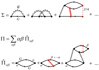
Figure 2: (Color online) Typical low-order diagrams contributing to the particle self-energy and polarization operator within the $G^{2}W$-skeleton scheme (red color denotes spin-exchange coupling). Diagrams for $\Sigma$ and $\Pi$, in their turn, are used to calculate fully dressed $G$ and $W$ functions, see Eq. (7).

To make connection with general rules of diagrammatic MC Prokof’ev and Svistunov (1998); Mishchenko et al. (2000) we formalize the problem at hand as computing quantity $Q(y,s)$ (where $y$ stands collectively for space, imaginary time, and spin variables, while $s=1,2$ labels the proper self-energy and the polarization operator sectors) from the series of multidimensional sums/integrals

$$Q(y,s)=\sum_{n\xi}\int dx_{1}...dx_{n}dY\;{\cal D}(n,\xi,\{x_{i}\};Y,s)\delta(y-Y)\;.$$ (9)

Here $n=0,1,\dots\infty$ is the diagram order, $\xi$ labels different terms of the same order, $x_{i}$ are internal integration/summation variables, and ${\cal D}$ is the diagram contribution to the answer. Formally, one can think of the set of skeleton diagrams for the free-energy of the system with one line marked as ’dummy’. When the dummy line is removed from the graph the rest is interpreted as a diagram for $\Sigma(y)$ (in this case $s=1$ and the dummy line is the particle propagator) or $\Pi(y)$ (in this case $s=2$ and the dummy line is the $\tilde{W}$ one). The last rule follows from the fact that $\Pi(y)$ is a continuous function of time. In the BDMC approach one interprets Eq. (9) as averaging of $e^{i\arg({\cal D})}\delta(y-Y)$ over the configuration space $\nu=(n,\xi,x_{1},\dots,x_{n};Y,s)$ with probability density proportional to $|{\cal D}|$.

The skeleton formulation does not cause any fundamental problem for Monte Carlo methods and is easy to implement for diagrams of arbitrary order. Essentially, at any stage in the calculation both $G$ and $W$ are considered to be known functions (the calculation may start with $G=G^{(0)}$ and $W=J/4$) while Eq. (7) is used from time to time to improve one’s knowledge about $G$ and $W$ using accumulated statistics for $\Sigma$ and $\Pi$ and fast Fourier transform algorithms. Moreover, we have shown Prokof’ev and Svistunov (2007) that BDMC methods are more stable and have better convergence properties than conventional iterations. One immediately recognizes that in the skeleton-type formulation (i) the number of diagrams to be sampled in a given order is dramatically reduced, (ii) the convergence of the skeleton series is likely to be different than that of the bare series, (iii) non-analytic and non-perturbative behavior might emerge even from a finite number of terms due to highly non-linear self-consistent formulation (we refer here to the famous mean-field BCS solution).

The other crucial advantage of BDMC over more conventional MC methods simulating finite clusters of spins is that it deals directly with the thermodynamic limit of the system. In practice, in dimension $d>1$ the error bars often become too large before a reliable extrapolation to the thermodynamic limit can be done. In this sense, BDMC is not subject to the infamous sign-problem which is understood as exponential scaling of computational complexity with the space-time volume of the physical system. Feynman diagrams do alternate in sign and contributions from high-order diagrams cancel each other to near zero. However, this behavior is better characterized as a ’sign-blessing’, not a sign-problem, because it is crucial for convergence properties. With the number of graphs growing factorially with their order the only possibility for obtaining series with finite convergence radius is to have sign-alternating terms such that high-order diagrams cancel each other (the sign-blessing phenomenon). For series with finite convergence radius there are numerous unbiased re-summation techniques which allow one to determine the answer well outside of the convergence radius provided enough terms in the series are known. Relatively small configuration space for skeleton diagrams allows one to establish if sign-blessing takes place in a given model and to obtain accurate results for diagram orders as large as 7-10 (depending on the model).

It should be noted that in recent years the Popov-Fedotov trick has become popular within the functional renormalization group (PFFRG) framework. It has been applied to frustrated $J_{1}-J_{2}$ model on square lattice Reuther and Wölfle (2010), planar $J_{1}-J_{2}-J_{3}$ antiferromagnet Reuther et al. (2011a), spatially anisotropic triangular antiferromagnet Reuther and Thomale (2011), and honeycomb lattice antiferromagnet with competing interactions Reuther et al. (2011b). These studies also attempt at attacking the problem using Feynman diagrammatic series but are radically different in the technical implementation. While PFFRG is also based on sums of subsets of selected diagrams to infinite order, it does not offer a convenient way to check for convergence of final results as more and more diagrams are retained. This is the most severe drawback of PFFRG; after all the major problem with existing theories is reliable estimate of the accuracy. The PFFRG spectral functions are very broad in energy Reuther and Wölfle (2010) and appear to underestimate ordering fluctuations. This also leads to significant rounding of susceptibility peaks and makes identification of different phases difficult. In addition, these studies are typically focused on the zero-temperature phase diagram, not the finite-temperature cooperative paramagnet state.

IV Normalization and worm-algorithm updates

To simplify notations let us write the diagrammatic contribution from the configuration space point $\nu$ as ${\cal D}_{\nu}=e^{i\varphi_{\nu}}D_{\nu}$ and call the non-negative function $D_{\nu}$ the configuration ’weight’. Within the $G^{2}W$-skeleton scheme $D_{\nu}$ is given by the modulus of a product which runs over all lines

$$D_{\nu}=|\prod_{\rm lines}f_{\rm line}(\nu)|\;,$$ (10)

where $f_{\rm line}(\nu)$ stands for a collection of functions describing various lines in the diagram. At this point we notice that equation

$$Q(y,s)=\sum_{\nu}e^{\varphi_{\nu}}D_{\nu}\delta(y-Y)\;.$$ (11)

can be always interpreted as averaging over the probability density distribution $P_{\nu s}=D_{\nu}/C_{s}$, where $C_{s}$ is the normalization factor, and thus sampled by MC methods:

$$Q(y,s)=C_{s}\sum_{\nu}e^{i\varphi_{\nu}}\delta(y-Y)P_{\nu s}\longrightarrow C_{s}\sum_{\nu}^{\text{M}C}e^{i\varphi_{\nu}}\delta(y-Y)\;.$$ (12)

In the last transformation we replace the full sum over the configuration space with the stochastic sum over configurations which are generated from the probability density $P_{\nu s}$. This is, of course, nothing but the standard MC approach to deal with complex multi-dimensional spaces. We stress here that all configuration parameters are sampled stochastically, including the diagram order and its structure, making Diagrammatic MC radically different from calculations which first create a list of all diagrams up to some high-order and then evaluate them one-by-one (often with the use of MC methods for doing the integrals).

IV.1 Normalization

The normalization constant $C$ can be determined in a number of ways:
(i) using known behavior of $Q(y,s)$ in some limiting case, for example $Q(y\to y_{0},s)\to Q_{0}(s)$,
(ii) through the exact sum rule, $\int dyQ(y,s)=R_{s}$, if available, or, more generically,
(iii) by measuring the ratio between the contributions of all diagrams in Eq. (9) and diagrams which are known either analytically or numerically with high accuracy. Indeed, imagine that one or several diagrams, say the lowest order ones, are known and their integrated contribution to the answer is $Q_{N}(s)=\int dyQ_{N}(y,s)$. Let ${\cal N}_{s}$ be their configuration space. Then the ratio $Q(y,s)/Q_{N}(s)$ can be measured in the MC simulation as

$$\left[\int dyQ(y,s)\right]/Q_{N}(s)=(\sum_{\nu}^{\text{M}C}e^{i\varphi_{\nu}})/(\sum_{\nu}^{\text{M}C}\delta_{\nu\in{\cal N}_{s}}\;e^{i\varphi_{\nu}})\;.$$ (13)

This leads to

$$C_{s}=\frac{Q_{N}(s)}{Z_{s}}\;,\qquad\qquad Z_{s}=\sum_{\nu}^{\text{M}C}\delta_{\nu\in{\cal N}_{s}}\;e^{i\varphi_{\nu}}\;.$$ (14)

The diagrams used for normalization are not necessarily the physical ones, i.e. they can be artificially “designed” to have simple analytic structure and added as a special sector to the configuration space $\{\nu\}$, see Ref. Prokof’ev and Svistunov, 2007. In the latter case, the diagrams contributing to $Q(y,s)$ and $Z_{s}$ are mutually exclusive and physical contributions have to be filtered by $(1-\delta_{\nu\in{\cal N}_{s}})$.

In the present study we use the modulus of the Hartree diagram to normalize statistics for $\Sigma$, and the modulus of the lowest order GG-diagram, see the first term in Fig. 2, to normalize statistics for $\Pi$:

$$Q_{N}(1) = \Sigma_{N}=\sum_{r}\sum_{\alpha}|\frac{J(r)}{4}|\,|G(\tau=-0)|\;,$$

$$Q_{N}(2) = \Pi_{N}=\sum_{\alpha}\int_{0}^{1/T}d\tau|G(\tau)G(-\tau)|\;.$$ (15)

Even though in the self-consistent scheme one does not know the $G(\tau)$-function analytically (it is tabulated numerically) it takes no time to compute the normalization factor $\Pi_{N}$ with high accuracy. We take the modulus of the Hartree diagrams because in the absence of external magnetic field the spin-up and spin-down contribution exactly cancel each other. Correspondingly,

$$Z_{1} = \sum_{\nu}^{\text{M}C}\delta_{\nu,({\rm Hartree},s=1)}\;,$$

$$Z_{2} = \sum_{\nu}^{\text{M}C}\delta_{\nu,(n=1,s=2)}\;.$$ (16)

IV.2 Worm-algorithm trick

We now proceed with the description of updates which ensure that all points in the configuration space are sampled from the probability density $P_{\nu s}$. Among many possibilities we seek a scheme which involves the smallest number of lines in a single update and does not require global analysis of the diagram structure. Such updates are called ”local”. Typically, they are much more flexible in design, are easier to implement, and lead to more efficient codes by having large acceptance ratios. The reader not interested in algorithmic details may proceed directly to the next Section.

An easy way to ensure that the diagram is irreducible is to check that no two lines in the graph have the same momentum—by momentum conservation laws the isolated self-energy blocks cannot change the line momentum. By creating a hash table where momenta of all lines are registered according to their values one can readily verify that momenta of updated lines are not repeated in the graph without looking at the graph topology or addressing all other lines. This simple tool solves the problem of performing local updates within the irreducible set. It can be applied even if diagrams are sampled in the real-space representation, as is done in this article, by attaching an auxiliary momentum variable to each line and satisfying the momentum conservation law at each vertex. In this case, the sole purpose of introducing auxiliary momenta is an efficient monitoring of the diagram topology and the ${\cal D}_{\nu}$ value is independent of them.

Since the trick with auxiliary momenta is based on momentum conservation laws one is necessarily limited to either (i) performing updates on closed loops, i.e. partially abandoning the idea of local updates, or (ii) extending the configuration space to include diagrams which violate these conservation laws. The second strategy is the essence of the worm algorithm. One more reason for using the worm algorithm approach is the spin projection conservation law in the interaction process, see Eq. (II) and Fig. 1. It also requires that updates are performed only on closed loops of interaction lines and propagators, unless one admits diagrams which violate the corresponding conservation law. It turns out that a straightforward extension of the worm algorithm introduced in Refs. Van Houcke et al., 2008 and Kozik et al., 2010 allows one to go around both hurdles.

The additional (unphysical) diagrams have the following structure. There are two special vertexes, or ’worms’, ${\cal S}$ and ${\cal T}$, where momentum and spin conservation laws are violated, see Fig. 3. In a given graph, any two vertexes can be special if they are not connected by the interaction line. Conservation laws become satisfied if one imagines a special line connecting ${\cal S}$ to ${\cal T}$. This line is not associated with any propagator and its mission is to transfer momentum $p_{w}$ and spin projection $1$ (doted line in Fig. 3); otherwise special vertexes represent a drain and a source of momentum $p_{w}$ and spin projection $1$, see Figs. 3 and 4. It has to be realized that the spin conservation law is formulated for a pair of vertexes connected by the interaction line, i.e. an interaction line containing a worm on one of its ends is unphysical and can be described by any suitable function $F(r,\tau)$.

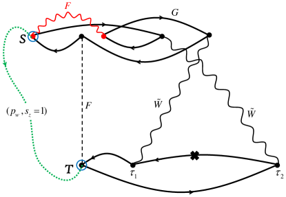
Figure 3: (Color online) Non-physical diagram with two special vertexes (worms) ${\cal S}$ and ${\cal T}$ (marked by blue circles). Momentum and spin conservation laws would be satisfied at all vertexes and interaction lines if one considers ${\cal S}$/${\cal T}$ as a drain/source of momentum $p_{w}$ and spin projection $1$; the same rule is recovered by imagining a line (green dotted) which carries $(p_{w},s_{z}=1)$ from ${\cal S}$ to ${\cal T}$. If special vertexes were not present in the diagram, then this graph would contribute to $\Sigma(\tau_{1}-\tau_{2})$ after removing the dummy propagator line marked by the cross (if cross marks the dummy $\tilde{W}$-line then the diagram is contributing to $\Pi$).

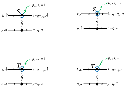
Figure 4: (Color online) Detailed structure of ${\cal S}$ and ${\cal T}$ vertexes. Note, that the interaction line containing a worm on one of its ends is also unphysical and the spin conservation law applies to a pair of vertexes.

The worm algorithm idea is based on the observation that updates performed with the use of special vertexes can always be made local, including non-trivial changes in the diagram topology and order as well as transformations replacing diagonal interaction lines with spin-flip ones. Even though unphysical diagrams are frequently encountered in the simulation process they are excluded from the statistics of $\Sigma$ and $\Pi$ which is accumulated only on the physical set of diagrams.

IV.3 Updates

Below we describe the simplest ergodic updating scheme. With trivial modifications and additional filters for proposals which would be rejected because they are incompatible with the allowed configuration space it can be made more efficient. This, however, would overwhelm the presentation with minor programming details and we choose not to discuss them here. For example, below we will use the following algorithmic rules for dummy lines used to identify diagrams as $\Sigma$- or $\Pi$-type: (i) the dummy interaction line cannot be removed or created in any update, (ii) if the dummy propagator originating from vertex ${\cal A}$ is modified by adding/removing an intermediate vertex ${\cal C}$ then ${\cal A}$ always remains the originating vertex of the new dummy line. These rules can be easily modified to avoid fast rejections of updates in certain cases at the expense of using additional random numbers to deal with available choices and taking care of them in acceptance ratios. Alternatively, the notion of the dummy line can be avoided altogether by designing an improved estimator based on free-energy diagrams.

Create - Delete

The pair of complementary updates Create - Delete switches between physical and unphysical sectors by inserting/removing a pair of special vertexes connected by the particle propagator. It is not allowed to have ${\cal S}$ = ${\cal T}$ or to have ${\cal S}$ and ${\cal T}$ being connected by the interaction line, see an illustration in Fig. 5. In Create, the particle propagator for update and the type of special vertex to be placed at its origin (${\cal A}\to{\cal S}$ or ${\cal A}\to{\cal T}$) are selected at random. One has to verify that flipping the propagator spin is consistent with the worm rules or reject the proposal. The missing momentum $p_{w}$ at the worm vertex is selected at random. In Delete, one selects a worm at random, checks that the outgoing particle propagator arrives at the other worm, and proposes to remove worms from the diagram. The corresponding acceptance ratios are given by

$$R_{\rm Create}=\frac{D_{\nu^{\prime}}}{D_{\nu}}\,\frac{u_{2}}{u_{1}}\,2n\,\;,\;R_{\rm Delete}=\frac{D_{\nu^{\prime}}}{D_{\nu}}\,\frac{u_{1}}{u_{2}}\,\frac{1}{2n}\;,$$ (17)

where $n$ is the diagram order and $\nu$ and $\nu^{\prime}$ are configuration space points before and after the update and $D_{\nu}$ is the product in Eq. (10). In the present case only one propagator and two interaction lines are affected:

$$\frac{D_{\nu^{\prime}}}{D_{\nu}}=\left|\frac{G_{AB}(\alpha)F_{SC}F_{TD}}{G_{AB}(-\alpha)W_{AC}W_{BD}}\right|\,,$$ (18)

in Create and similarly, $D_{\nu^{\prime}}/D_{\nu}=|GWW/GFF|$, in Delete with appropriate arguments for all functions involved. [If the line is labeled as $W$ it can be either of $J$ or $\tilde{W}$ type.] In what follows we will stop mentioning which vertexes determine function parameters since these can be easily recovered from the figures. Finally, assuming that the protocol of deciding which update should be implemented next is random and based on assigning each update some probability, $u_{i}$, we mention the ratio of probabilities in the acceptance ratio ($u_{1}$ for Create and $u_{2}$ for Delete).

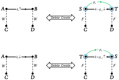
Figure 5: Two cases for Create and Delete updates which insert/remove a pair of worms at the ends of the particle propagator.

Create-H - Delete-H

This pair of complementary updates also switches between physical and unphysical sectors with an additional ingredient—it increases/decreases the diagram order by attaching a Hartree-type bubble to the existing graph. According to the rule ’no two lines may have the same momentum’ the diagram remains irreducible because one of the worms is placed on the bubble vertex. The overall transformation is illustrated in Fig. 6; the text below addresses to this figure with regards to the procedure of selecting specific graph parameters. In Create-H a particle propagator (going from vertex ${\cal A}$ to vertex ${\cal B}$) and whether to place ${\cal S}$ or ${\cal T}$ on vertex ${\cal B}$ is decided at random. If the proposal is inconsistent with the worm rules it has to be rejected. Next, a new time variable for the intermediate vertex ${\cal C}$ is generated from the probability density, $t(\tau)$, and a random decision is made whether the new interaction line is of the $J$- or $\tilde{W}$-type. For the $J$-line (with $\tau^{\prime}=\tau$) the position of the second worm vertex in space is obtained from the normalized $X(r^{\prime})\propto J(r^{\prime})$ distribution. For the $\tilde{W}$-line this position is obtained from some designed probability distribution $Y(r^{\prime})$ while the time location is drawn from the probability density, $t(\tau^{\prime})$. The spin variable in the bubble, the bubble momentum variable $p$ and the worm momentum $p_{w}$ are decided at random. In Delete-H a random choice is made what type of special vertex must be on the Hartree bubble provided the overall topology of lines is identical to that on the r.h.s of Fig. 6. The proposal is to remove worms and the bubble from the diagram. It is rejected if either the propagator originating from ${\cal C}$ or the interaction line attached to ${\cal C}$ is the dummy one. The acceptance ratios for these updates are (probabilities of calling Create-H are Delete-H are $u_{3}$ and $u_{4}$, respectively)

$$R_{\rm Create-H}=\frac{D_{\nu^{\prime}}}{D_{\nu}}\frac{u_{4}}{u_{3}}\frac{2^{3}n}{t(\tau)}\left\{\begin{array}[]{ll}1/X(r^{\prime});&\;\;(J)\\ 1/Y(r^{\prime})t(\tau^{\prime});&\;\;(\tilde{W})\end{array}\right.$$ (19)

$$R_{\rm Delete-H}=\frac{D_{\nu^{\prime}}}{D_{\nu}}\frac{u_{3}}{u_{4}}\frac{t(\tau)}{2^{3}(n-1)}\left\{\begin{array}[]{ll}X(r^{\prime});&\;\;(J)\\ Y(r^{\prime})t(\tau^{\prime});&\;\;(\tilde{W})\end{array}\right.$$ (20)

with the diagram weight ratios $D_{\nu^{\prime}}/D_{\nu}$ given by $|GGFFG/GW|$ and $|GW/GGFFG|$ in Create-H and Delete-H, respectively (note that here $n$ is the initial diagram order). The simplest choices for probability distributions in Eqs.(19) and (20) would be uniform distributions $t(\tau)=T$, $X(r^{\prime})=1/z$, and $Y(r^{\prime})=1/V$, where $V$ is the total number of lattice sites. One can use other functions for better acceptance ratio.

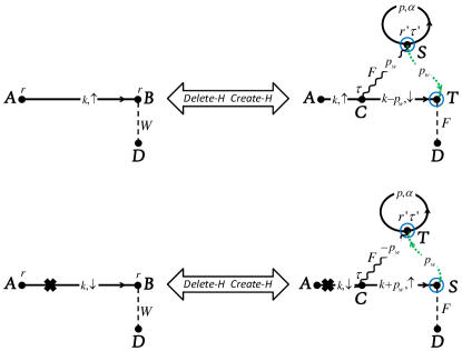
Figure 6: Two cases for Create-H and Delete-H updates which insert/remove a pair of worms and increase the diagram order by adding a Hartree-type bubble.

The three updates described next represent a random diffusion of special vertexes along the graph lines (this places ${\cal S}$ and ${\cal T}$ on any allowed pair of vertexes) supplemented by an update which changes the graph topology.

Move-P

In this self-complementary update one selects at random ${\cal S}$ or ${\cal T}$ and proposes to shift the selected worm along the incoming or outgoing propagator line, deciding again randomly between the two choices. Since all four case are identical in their implementation we describe below an update shifting ${\cal S}$ along the outgoing propagator line to vertex B, see upper panel in Fig. 7, if ${\cal B}\neq{\cal S}$, of course. According to the rules, if ${\cal B}={\cal T}$, or ${\cal D}={\cal T}$, or the spin of the outgoing line is down, the update is rejected. Finally, one has to check whether the proposal may lead to the irreducible diagram. For the update shown in Fig.7 the acceptance ratio is given by

$$R_{\rm Move-P}=\left|\frac{GWF}{GFW}\right|\;.$$ (21)

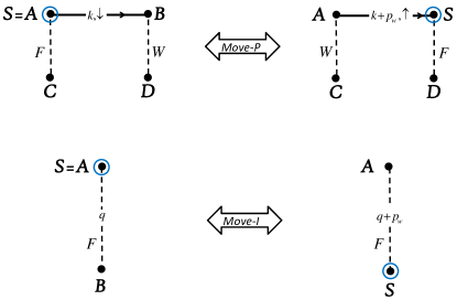
Figure 7: Upper panel: An illustration of the Move-P update shifting ${\cal S}$ along the propagator line. This move changes the momentum of the propagator line and flips its spin as well as the status of interaction lines between physical and unphysical. Lower panel: An illustration of the Move-I update shifting ${\cal S}$ along the interaction line. This move changes the auxiliary momentum of the interaction line only.

Move-I

In this self-complementary update one selects at random ${\cal S}$ or ${\cal T}$ and proposes to shift the selected worm along the interaction line to vertex ${\cal B}$, see the lower panel in Fig. 7. One has to check whether the proposal may lead to the irreducible diagram. This update is always accepted since it changes only the auxiliary momentum variable.

Commute

All possible topologies in a graph of order $n$ can be generated by randomly connecting outgoing propagator lines to incoming ones. Having this observation in mind the self-complementary Commute update proposes to swap destination vertexes for propagator lines originating at ${\cal S}$ or ${\cal T}$, see Fig. 8. This proposal is valid only if all vertexes have the same space coordinate and both propagators have the same spin index. The crucial advantage of the worm algorithm at this point becomes clear—momentum conservation law is satisfied by absorbing the difference $k-p$ into the worm momentum $p_{w}\to p_{w}+k-p$. This update is accepted with ratio

$$R_{\rm Commute}=\left|\frac{GG}{GG}\right|\;.$$ (22)

In the lower panel of Fig. 8 we show a typical diagram change produced by Commute. It always changes the number of fermionic loops in the graph and, in particular, will transform a diagram with a bubble attached to the worm vertex into the vertex-correction type diagram. This explains, to some extent, our design of updates Create-H and Delete-H.

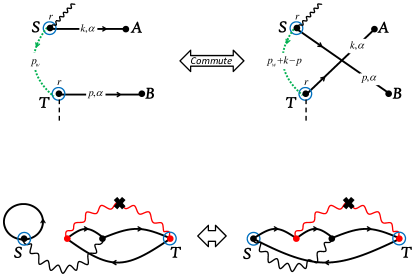
Figure 8: Upper panel: In the Commute update the diagram topology is changed by re-directing propagators originating at special vertexes ${\cal S}$ and ${\cal T}$ to have their destination vertexes at ${\cal B}$ and ${\cal A}$, respectively. Lower panel: typical transformation produced by the Commute update.

Dummy

To place the dummy line mark on any of the $G$- or $\tilde{W}$-lines we select one of the vertexes at random, say vertex ${\cal A}$, and make a random decision whether the new dummy line should be the interaction line attached to ${\cal A}$ (it has to be of the $\tilde{W}$ type) or the propagator line originating from ${\cal A}$. The proposal is always accepted if the notion of the dummy mark does not change the value of the function behind the line (which is assumed to be the case here).

The above set of updates is sufficient for doing the simulation. It can always be supplemented by additional updates which do not necessarily involve special vertexes but reduce the autocorrelation time and lead to more efficient sampling of the diagram variables. Moreover, a non-trivial check of the detailed balance for debugging purposes is only possible if the set of updates is overcomplete. Below we describe several such updates.

Insert-Remove

An idea here is to increase/decrease the diagram order by inserting/removing a ladder-type structure. More precisely, in Insert we make a random choice between ${\cal S}$ and ${\cal T}$ to start the construction from the special vertex ${\cal V}_{1}$. Next we identify vertex ${\cal A}$ as the destination vertex of the propagator originating from ${\cal V}_{1}$, and vertex ${\cal B}$ as the originating vertex for the propagator with the destination vertex ${\cal V}_{2}$, which is the other worm end, see the upper panel in Fig. 9. If ${\cal A}={\cal V}_{2}$ the update is rejected. The proposal is to insert new vertexes ${\cal C}$ (intermediate between ${\cal V}_{1}$ and ${\cal A}$) and ${\cal D}$ (intermediate between ${\cal B}$ and ${\cal V}_{2}$) and to link them with the interaction line of randomly chosen type, either $J$ or $\tilde{W}$, and momentum $q$. The new time variables are generated from the probability density $t(\tau)$. The momenta of new lines and the worm are modified as described in Fig. 9 to satisfy conservation laws. Finally, if one of the propagators is the dummy line, the new dummy line has to have the same originating vertex. In Remove we select one of the special vertexes, ${\cal V}_{1}$, at random and verify that the topology of lines connecting it to the other special vertex, ${\cal V}_{2}$, as well as lines parameters are consistent with Fig. 9 (upper panel). If either ${\cal C}$-${\cal A}$ or ${\cal D}$-${\cal V}_{2}$ propagator is a dummy line the update is rejected. The proposal then is to remove vertexes ${\cal C}$ and ${\cal D}$ from the graph and update momenta of the lines accordingly. The acceptance ratios are given by

$$R_{\rm Insert}=\frac{D_{\nu^{\prime}}}{D_{\nu}}\frac{u_{10}}{u_{9}}\frac{2}{t(\tau)}\left\{\begin{array}[]{ll}1;&\;\;(J)\\ 1/t(\tau^{\prime});&\;\;(\tilde{W})\end{array}\right.$$ (23)

$$R_{\rm Remove}=\frac{D_{\nu^{\prime}}}{D_{\nu}}\frac{u_{9}}{u_{10}}\frac{t(\tau)}{2}\left\{\begin{array}[]{ll}1;&\;\;(J)\\ t(\tau^{\prime});&\;\;(\tilde{W})\end{array}\right.$$ (24)

where $D_{\nu^{\prime}}/D_{\nu}=|GGGGW/GG|$ in Insert and its inverse in Remove.

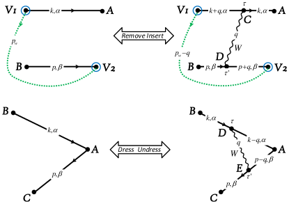
Figure 9: Upper panel: Increasing/decreasing the diagram order using a pair of complementary updates Insert and Remove. When the propagators ${\cal V}_{1}$-${\cal A}$ and ${\cal B}$-${\cal V}_{2}$ are linked with the new interaction line ${\cal C}$-${\cal D}$ carrying momentum $q$ the closed loop for momentum conservation goes as ${\cal V}_{1}$-${\cal C}$-${\cal D}$-${\cal V}_{2}$-${\cal V}_{1}$. The same loop is used in the Remove update. Lower panel: Diagram transformation when vertexes are dressed and undressed with interaction lines.

Dress-Undress

One of the easiest updates to increase the diagram order within the $G^{2}W$-skeleton formulation is to dress an existing vertex with interaction line and consider the smallest closed loop for transferring momentum. The Dress update starts from random selection of vertex ${\cal A}$ and identification of vertexes ${\cal B}$ and ${\cal C}$ linked to it by propagator lines; if ${\cal B}={\cal A}$ the update is rejected (we pay no attention in this update whether one of the vertexes is of a special type). The proposal is to add new vertexes ${\cal D}$ (intermediate between ${\cal B}$ and ${\cal A}$) and ${\cal E}$ (intermediate between ${\cal A}$ and ${\cal C}$) and to link them with the $\tilde{W}$ line with random momentum $q$. The new time variables are generated from the probability density $t(\tau)$. The momenta of new lines are modified as described in the lower panel of Fig. 9 to satisfy conservation laws. In Undress we select vertex ${\cal A}$ at random, identify vertexes ${\cal D}$, ${\cal B}$, ${\cal E}$, and ${\cal C}$ using links along the propagator lines, and verify that the topology of lines and their parameters are consistent with the dressed vertex configuration. If the ${\cal D}$-${\cal E}$ line is not of the diagonal $\tilde{W}$ type or one of the propagators ${\cal D}$-${\cal A}$ or ${\cal E}$-${\cal C}$ is a dummy line, the update is rejected. The proposal is to remove vertexes ${\cal D}$ and ${\cal E}$ from the graph. The acceptance ratios are

$$R_{\rm Dress}=\frac{D_{\nu^{\prime}}}{D_{\nu}}\frac{u_{12}}{u_{11}}\frac{n}{(n+1)t(\tau)t(\tau^{\prime})}\;,$$ (25)

$$R_{\rm Undress}=\frac{D_{\nu^{\prime}}}{D_{\nu}}\frac{u_{12}}{u_{11}}\frac{n}{(n-1)t(\tau)t(\tau^{\prime})}\;,$$ (26)

where $D_{\nu^{\prime}}/D_{\nu}=|GGGGW/GG|$ in Dress and its inverse in Undress.

Recolor

An easy and efficient way to change the spin index of propagator lines is to select a random vertex and use it to construct a closed loop by following the propagator lines attached to it. If all propagators in the loop have the same spin index $\alpha$ it can be changed to $-\alpha$ with acceptance ratio unity in the absence of external magnetic field; otherwise, one has to use the ratio of products of all propagator lines after and before the update.

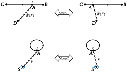
Figure 10: An illustration of the Move-T update changing the imaginary time location of a randomly chosen vertex. One is free to change the type of worm from ${\cal S}$ to ${\cal T}$ or to place it on any of the vertexes in both panels.

Move-T

This self-complementary update is designed to sample time variables of the diagram without changing its order and topology. The proposal is to select one of the vertexes at random, let it be vertex ${\cal A}$ and update its imaginary time variable from $\tau$ to $\tau^{\prime}$ using probability density distribution $t(\tau^{\prime})$, see Fig. 10 for two alternatives. The interaction line attached to ${\cal A}$ cannot be of the $J$-type; whether it is the physical $\tilde{W}$-line or unphysical $F$-line does not mater. The acceptance ratio is given by

$$R_{\rm Move-T}=\frac{t(\tau)}{t(\tau^{\prime})}\begin{cases}|\tilde{W}(F)/\tilde{W}(F)|\,|GG/GG|&\text{(generic)}\\ |F/F|&\text{(bubble)}\end{cases}.$$ (27)

IV.4 Diagram sign

With the dummy line removed, the diagram phase required to compute the self-energy and polarization operator using Eqs. (12) and (14) is determined by standard diagrammatic rules (see also Eq. (10)):

$$\varphi_{\nu}=\sum_{\rm lines}\arg(f_{\rm line}(\nu))+\pi(n+l)\;,$$ (28)

where $l$ is the number of fermionic loops (one only needs to know whether it is even or odd). This phase is readily recalculated in updates without addressing the whole diagram since $l$ always changes its parity when Create-H, Delete-H, and Commute are accepted.

IV.5 Satisfying the sum rule

The value of the spin-spin correlation function $\chi(r=0,\tau=0)=\langle(S^{z})^{2}\rangle=1/4$, see Eq. (4), provides an important sum rule in the Fourier space

$$T\sum_{n}\int_{BZ}\frac{d{\mathbf{q}}}{8\pi^{2}/\sqrt{3}}\chi(q,n)=1/4\;,$$ (29)

which can be used for modifying convergence properties of the self-consistent scheme as follows (the integral is taken over the Brillouin zone (BZ)). When the maximum diagram order is fixed at $N$ the sum rule is violated by some amount which vanishes as $N\to\infty$. Since the final result is claimed after taking the limit, it is perfectly reasonable to impose a condition that the sum rule is always satisfied by scaling $\Pi$ by an appropriate factor. This is exactly what is done in this article: after solving the Dyson Equation we check the value of $\chi(r=0,\tau=0)$, adjust the scaling factor for $\Pi$, and go back to solving the Dyson Equation again until the sum rule is satisfied with three digit accuracy.

V Triangular lattice Heisenberg antiferromagnet

In the diagrammatic formulation there is no conceptual difference in the implementation of the numerical scheme for any dimension of space, lattice type, and interaction range. Thus, sign-problem free systems, e.g. the square/cubic lattice Heisenberg antiferromagnet with nearest neighbor coupling, can be used for testing purposes since their properties are known with high degree of accuracy (with reliable extrapolation to the thermodynamic limit) using path-integral and stochastic series expansion MC methods. After passing such tests, we turn our attention to the triangular-lattice Heisenberg antiferromagnet (TLHA) which is a canonical frustrated magnetic system with massively degenerate ground state in the Ising limit.

The most important question to answer is whether the sign blessing phenomenon indeed takes place, i.e. there is a hope for obtaining accurate predictions in the strong coupling regime by calculating higher-and-higher order diagrams despite factorial growth in the number of contributing graphs. In Fig. 11 we show comparison between the calculated answer for the static uniform susceptibility

$$\chi_{u}=\chi(q=0,m=0)=\int_{0}^{1/T}d\tau\sum_{r}\chi(r,\tau)\,,$$ (30)

and the high-temperature expansion results Zheng et al. (2005); Rigol et al. (2007) at $T/J=2$. This temperature is low enough to ensure that we are in the regime of strong correlations because $\chi_{u}$ is nearly a factor of two smaller than the free spin answer $\chi_{u}^{0}=1/4T$. On the other hand, this temperature is high enough to be sure that the high-temperature series can be described by Padé approximants without significant systematic deviations from the exact answer Zheng et al. (2005); Rigol et al. (2007) (at slightly lower temperature the bare NLC series start to diverge). We clearly see in Fig. 11 that the BDMC series converges to the correct result with accuracy of about three meaningful digits and there is no statistically significant change when more than a hundred thousand of 7-th order diagrams are accounted for. [We recall that the number of topologically distinct diagrams within the $G^{2}W$-skeleton scheme was calculated in Ref. L.G. Molinari and N. Manini, 2006; for the eight lowest orders they are $1,1,6,49,542,7278,113824,2017881$.] The error bar for the 7-th order point is significantly increased due to exponential growth in computational complexity. The 4-th order result can be obtained after several hours of CPU time on a single processor.

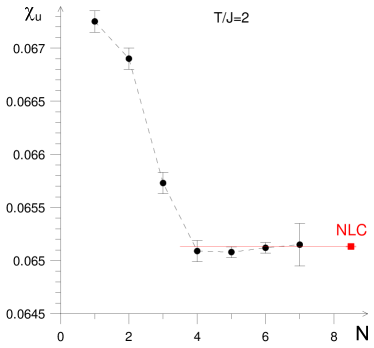
Figure 11: (Color online) Uniform susceptibility calculated within the $G^{2}W$-skeleton expansion as a function of the maximum diagram order retained in the BDMC simulation (black dots) for $T/J=2$. The result of the high-temperature expansion (with Padé approximant extrapolation) Zheng et al. (2005) is shown by red square and horizontal line.

Interestingly enough, when temperature is lowered down to $T/J=1$, which is significantly below the point where the bare NLC series start to diverge (see Fig. 13), the BDMC series continue to converge (see Fig. 12). This underlines the importance of performing simulations within the self-consistent skeleton formulation.

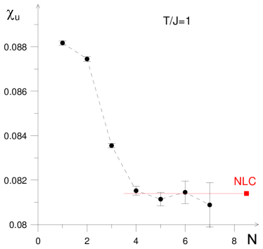
Figure 12: (Color online) Uniform susceptibility as a function of the maximum diagram order (black dots) for $T/J=1$. The result of the high-temperature expansion (with Padé approximant extrapolation) Zheng et al. (2005) is shown by red square and horizontal line. Its error bar is based on the difference between various expansion/extrapolation schemes.

In Fig. 13 we show results of the BDMC simulation performed at temperatures significantly below the mean-field transition temperature. For all points we observe extremely good agreement (essentially within our error bars) with the Padé approximants used to extrapolate the high-temperature expansion data to lower temperature Zheng et al. (2005). Within the current protocol of dealing with skeleton diagrams we were not able to go to lower temperature due to the development of singularity in the response function (and thus effective interaction $\tilde{W}$ at the wave-vector $Q=(4\pi/(3a),0)$. When the denominator $4-J(q)\Pi(q,m)$ in (7) is close to zero it becomes very difficult to control highly non-linear sets of coupled integral equations given finite statistical noise on the measured quantity $\Pi(q,m)$.

This is clearly seen in Fig. 14 where we show data for the staggered susceptibility $\chi(Q,0)$, defined as

$$\chi_{s}=\chi(Q,m=0)=\int_{0}^{1/T}d\tau\sum_{r}\;e^{iQ\cdot r}\chi(r,\tau)\,,$$ (31)

along with the Curie law and the uniform susceptibility, on the double logarithmic scale.

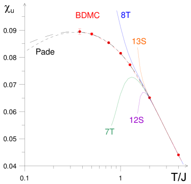
Figure 13: (Color online) Uniform susceptibility as a function of temperature (red dots) for the triangular Heisenberg antiferromagnet calculated within the BDMC approach. NLC expansion results  Rigol et al. (2007) based on triangles (labeled as 7T and 8T) and sites (labeled as 12S and 13S) are shown along with two different Padé approximant extrapolations of high-temperature expansions Zheng et al. (2005).

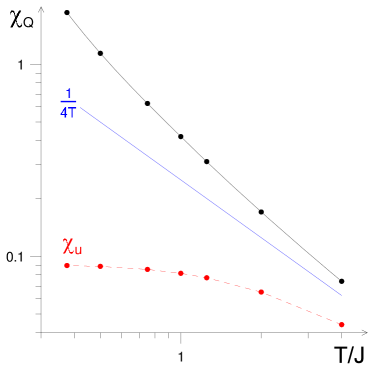
Figure 14: (Color online) Staggered susceptibility at the wave vector $Q$ as a function of temperature (black dots) plotted for comparison along with the Curie-Weiss law (blue curve) and uniform susceptibility (red dots and line).

One of the advantages of our approach is the ability to perform calculations of susceptibility at arbitrary momentum. In Fig. 15 we show data for $\chi(q,0)$ along the $\Gamma-K-M-\Gamma$ trajectory in the Brillouin zone (BZ). Here $\Gamma$ is the center of the BZ, $K=Q=(4\pi/(3a),0)$, and $M=(\pi/a,\pi/(\sqrt{3}a))$ is the mid-point on the face of the hexagonal BZ (see Fig. 15). Results presented in Figs. 14 and 15 are new because they are obtained for the static (zero Matsubara frequency) susceptibility in the thermodynamic limit. It is useful to note that the static response is far more difficult to get within the NLC method which is suited for calculations of the equal time correlation functions, such as, for example, equal time spin structure factor. The exception is represented by the uniform, or zero momentum, response which is based on the total magnetization commuting with the Hamiltonian. In addition, we can afford very high resolution in momentum space which is not the case for calculations based on clusters of finite size.

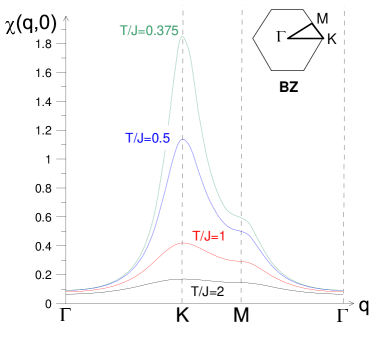
Figure 15: (Color online) Static spin-spin correlation function along the characteristic trajectory in the Brillouin zone.

It is clearly seen in Fig. 15 that around $T/J=1$ system’s response is enhanced along the whole Brillouin zone boundary indicative of the frustrated behavior. Only at temperatures below $T/J=0.5$ it becomes evident that the system wants to develop correlations commensurate with the K point. We confirm previous observation Elstner et al. (1993) that even at $T/J=0.375$ the spin correlation length, which can be estimated from the half-width of the peak around K point, is still of the order of lattice constant $a$. This can be checked even more explicitly by looking on the static spin correlations in real space. Figure 16 shows that while the sign structure of short-range spatial correlations is consistent with the three-sublattice $120^{\circ}$ state, the magnitude of the correlations becomes exponentially small on the scale of a few lattice periods. Closer look also reveals dramatic suppression of correlations between site $0$ (say, sublattice A) and sites $3$ and $7$ both of which would belong to sublattice C in the perfectly ordered $120^{\circ}$ classical state. Moreover, at slightly higher temperature $T/J=0.5$ the sign of correlations on sites $3$ and $7$ changes sign and turns ferromagnetic, similar to A-sublattice spins, though with much smaller amplitude. This temperature induced reversal of correlations is a remarkable effect specific for a frustrated system.

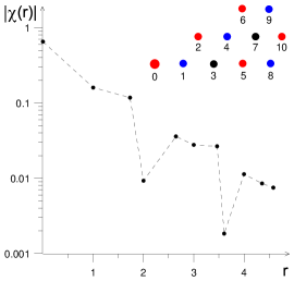
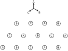
Figure 16: (Color online) Modulus of the spin susceptibility in real space at $T/J=0.375$ on the logarithmic scale. Lattice points are enumerated according to their distance from the origin. Spins on red sites (0, 2, 5, 6, 10) are correlated ferromagnetically while spins on blue and black sites are correlated anti-ferromagnetically with the spin at the origin. At slightly higher temperature $T/J=0.5$ black points (3, 7) start to correlate ferromagnetically with the spin $S_{0}$ at the origin, contrary to the classical ground state pattern depicted to the right.

It has been noted some time ago that short wavelength spin excitations contribute significantly to the finite temperature properties of triangular lattice antiferromagnet at not too low temperature Zheng et al. (2006). This has to do with substantial phase space volume these excitations occupy as well as with their relatively weak dispersion Starykh et al. (2006). It is conceivable that particularly weak correlations between sublattices A and C noted above have to do with these excitations as well. All of these features can be extracted from the retarded spin susceptibility $\chi(q,\omega)$ calculation of which requires analytic continuation of our Matsubara-frequency susceptibility $\chi(q,\omega_{m})$ to the real frequency. We plan to address this important issue in the near future.

VI Conclusions

This paper describes novel approach to frustrated spin systems. Obtained numerical results for the spin-1/2 triangular lattice Heisenberg model, Section V, show the power and competitiveness of our approach in comparison with other well established numeric techniques.

Future work has to address the issue of performing simulations at lower temperature in the regime characterized by the large correlation length. Technically, this translates into being close to zero in the denominator of Eq. (7) for some momentum values. Progress in this direction should allow us to better describe the cross-over/transition from the cooperative paramagnet to the long-range ordered (albeit frustrated) state.

Yet perhaps the most promising line of attack has to do with applying our technique to the geometrically frustrated models that do not support magnetically ordered state at all. In two dimensions this singles out quantum kagomé lattice antiferromagnet which have recently being shown to realize a long-sought $Z_{2}$ spin liquid state Yan et al. (2011). This task will require extension of our approach to systems with several (three in this case) spins in a unit cell. The added matrix complexity does not represent any fundamental difficulty.

Moving one dimension higher brings one to the most frustrated antiferromagnet in the world – spin-1/2 pyrochlore antiferromagnet Canals and Lacroix (1998); Moessner and Chalker (1998); Gardner et al. (2010). Pyrochlore Ising-like model realizes beautiful quantum spin-ice physics Ross et al. (2011) while the fate of spin-1/2 Heisenberg model is an open question. It is widely believed that ‘cooperative paramagnet’ region is most extended in this three-dimensional system. Unlike many lower-dimensional frustrated system, spin-1/2 pyrochlore is essentially not accessible by quantum Monte-Carlo technique due to large unit cell (4 spins). We believe that our Diagrammatic MC approach is therefore uniquely suited for studying the finite-temperature dynamics of this outstanding frustrated magnet.

Recently we have generalized the Popov-Fedotov trick to a universal technique of fermionization which leads to a well-defined standard diagrammatic technique for arbitrary lattice spin, boson, and fermion system with constraints on the on-site Fock states Prokof’ev and Svistunov (2011). This development creates a broader context for the present work: successful implementation of the BDMC method for models of quantum magnetism may lead to the universal numerical tool for arbitrary strongly correlated lattice models within the fermionization framework when diagrammatic expansion do not involve large parameters.

We thank M. Rigol for communicating us data obtained within the NLC method. This work was supported by the National Science Foundation under grants PHY-1005543 (S.K., N.P., B.S., and C.N.V.) and DMR-1206774 (O.A.S.), and by a grant from the Army Research Office with funding from the DARPA.

References

- Harris et al. (1997) M. J. Harris, S. T. Bramwell, D. F. McMorrow, T. Zeiske, and K. W. Godfrey, Phys. Rev. Lett. 79, 2554 (1997).
- Bramwell and Gingras (2001) S. T. Bramwell and M. J. P. Gingras, Science 294, 1495 (2001).
- Isakov et al. (2004) S. V. Isakov, K. Gregor, R. Moessner, and S. L. Sondhi, Phys. Rev. Lett. 93, 167204 (2004).
- Castelnovo et al. (2008) C. Castelnovo, R. Moessner, and S. Sondhi, Nature 451, 42 (2008).
- Pomeranchuk (1941) I. Y. Pomeranchuk, Zh. Eksp. Teor. Fiz. 11, 226 (1941).
- Balents (2010) L. Balents, Nature 464, 199 (2010).
- Hiroi et al. (2001) Z. Hiroi, M. Hanawa, N. Kobayashi, M. Nohara, H. Takagi, Y. Kato, and M. Takigawa, Journal of the Physical Society of Japan 70, 3377 (2001).
- Shimizu et al. (2003) Y. Shimizu, K. Miyagawa, K. Kanoda, M. Maesato, and G. Saito, Phys. Rev. Lett. 91, 107001 (2003).
- Okamoto et al. (2007) Y. Okamoto, M. Nohara, H. Aruga-Katori, and H. Takagi, Phys. Rev. Lett. 99, 137207 (2007).
- Itou et al. (2007) T. Itou, A. Oyamada, S. Maegawa, M. Tamura, and R. Kato, Journal of Physics: Condensed Matter 19, 145247 (2007).
- Itou et al. (2008) T. Itou, A. Oyamada, S. Maegawa, M. Tamura, and R. Kato, Phys. Rev. B 77, 104413 (2008).
- Olariu et al. (2008) A. Olariu, P. Mendels, F. Bert, F. Duc, J. C. Trombe, M. A. de Vries, and A. Harrison, Phys. Rev. Lett. 100, 087202 (2008).
- Yoshida et al. (2009) M. Yoshida, M. Takigawa, H. Yoshida, Y. Okamoto, and Z. Hiroi, Phys. Rev. Lett. 103, 077207 (2009).
- Okamoto et al. (2009) Y. Okamoto, H. Yoshida, and Z. Hiroi, Journal of the Physical Society of Japan 78, 033701 (2009).
- Mendels and Bert (2010) P. Mendels and F. Bert, Journal of the Physical Society of Japan 79, 011001 (2010).
- Nakatsuji et al. (2010) S. Nakatsuji, Y. Nambu, and S. Onoda, Journal of the Physical Society of Japan 79, 011003 (2010).
- Vachon et al. (2011) M.-A. Vachon, G. Koutroulakis, V. F. Mitrović, O. Ma, J. B. Marston, A. P. Reyes, P. Kuhns, R. Coldea, and Z. Tylczynski, New Journal of Physics 13, 093029 (2011).
- Quilliam et al. (2011) J. A. Quilliam, F. Bert, R. H. Colman, D. Boldrin, A. S. Wills, and P. Mendels, Phys. Rev. B 84, 180401 (2011).
- Yamashita et al. (2012) M. Yamashita, T. Shibauchi, and Y. Matsuda, ChemPhysChem 13, 74 (2012).
- Yan et al. (2012) Y. J. Yan, Z. Y. Li, T. Zhang, X. G. Luo, G. J. Ye, Z. J. Xiang, P. Cheng, L. J. Zou, and X. H. Chen, Phys. Rev. B 85, 085102 (2012).
- Anderson (1987) P. W. Anderson, Science 235, 1196 (1987).
- Wen (2002) X.-G. Wen, Phys. Rev. B 65, 165113 (2002).
- Kitaev (2006) A. Kitaev, Ann. Phys. 321, 2 (2006).
- Meng et al. (2010) Z. Y. Meng, T. C. Lang, S. Wessel, F. F. Assaad, and A. Muramatsu, Nature 464, 847 (2010).
- Varney et al. (2011) C. N. Varney, K. Sun, V. Galitski, and M. Rigol, Phys. Rev. Lett. 107, 077201 (2011).
- Dang et al. (2011) L. Dang, S. Inglis, and R. G. Melko, Phys. Rev. B 84, 132409 (2011).
- Yan et al. (2011) S. Yan, D. A. Huse, and S. R. White, Science 332, 1173 (2011).
- Isakov et al. (2011) S. V. Isakov, M. B. Hastings, and R. G. Melko, Nat. Phys. 7, 772 (2011).
- Okumura et al. (2010) S. Okumura, H. Kawamura, T. Okubo, and Y. Motome, Journal of the Physical Society of Japan 79, 114705 (2010).
- Yao and Kivelson (2012) H. Yao and S. A. Kivelson, Phys. Rev. Lett. 108, 247206 (2012).
- Ramirez (1994) A. P. Ramirez, Ann. Rev. Mat. Sci. 24, 453 (1994).
- Sachdev (1999) S. Sachdev, Quantum Phase Transitions (Cambridge University Press, Cambridge, 1999).
- Popov and Fedotov (1988) V. N. Popov and S. A. Fedotov, Sov. Phys. - JETP 67, 535 (1988).
- Popov and Fedotov (1991) V. N. Popov and S. A. Fedotov, Proc. Steklov Inst. Math. 177, 184 (1991).
- Prokof’ev and Svistunov (2007) N. Prokof’ev and B. Svistunov, Phys. Rev. Lett. 99, 250201 (2007).
- Kozik et al. (2010) E. Kozik, K. V. Houcke, E. Gull, L. Pollet, N. Prokof’ev, B. Svistunov, and M. Troyer, EPL (Europhysics Letters) 90, 10004 (2010).
- Van Houcke et al. (2012) K. Van Houcke, F. Werner, E. Kozik, N. Prokof’ev, B. Svistunov, M. J. H. Ku, A. T. Sommer, L. W. Cheuk, A. Schirotzek, and M. W. Zwierlein, Nat. Phys. 8, 366–370 (2012).
- Rigol et al. (2007) M. Rigol, T. Bryant, and R. R. P. Singh, Phys. Rev. E 75, 061118 (2007).
- Zheng et al. (2005) W. Zheng, R. R. P. Singh, R. H. McKenzie, and R. Coldea, Phys. Rev. B 71, 134422 (2005).
- Prokof’ev and Svistunov (2011) N. V. Prokof’ev and B. V. Svistunov, Phys. Rev. B 84, 073102 (2011).
- Fetter and Walecka (1971) A. Fetter and J. Walecka, Quantum Theory of Many-Particle Systems (McGraw-Hill, New York, 1971).
- Prokof’ev and Svistunov (1998) N. V. Prokof’ev and B. V. Svistunov, Phys. Rev. Lett. 81, 2514 (1998).
- Mishchenko et al. (2000) A. S. Mishchenko, N. V. Prokof’ev, A. Sakamoto, and B. V. Svistunov, Phys. Rev. B 62, 6317 (2000).
- Reuther and Wölfle (2010) J. Reuther and P. Wölfle, Phys. Rev. B 81, 144410 (2010).
- Reuther et al. (2011a) J. Reuther, P. Wölfle, R. Darradi, W. Brenig, M. Arlego, and J. Richter, Phys. Rev. B 83, 064416 (2011a).
- Reuther and Thomale (2011) J. Reuther and R. Thomale, Phys. Rev. B 83, 024402 (2011).
- Reuther et al. (2011b) J. Reuther, D. A. Abanin, and R. Thomale, Phys. Rev. B 84, 014417 (2011b).
- Van Houcke et al. (2008) K. Van Houcke, E. Kozik, N. Prokof’ev, and B. Svistunov, “Diagrammatic Monte Carlo,” in Computer Simulation Studies in Condensed Matter Physics XXI, edited by D. Landau, S. Lewis, and H. Schuttler (Springer Verlag, Heidelberg, Berlin, 2008).
- L.G. Molinari and N. Manini (2006) L.G. Molinari and N. Manini, Eur. Phys. J. B 51, 331 (2006).
- Elstner et al. (1993) N. Elstner, R. R. P. Singh, and A. P. Young, Phys. Rev. Lett. 71, 1629 (1993).
- Zheng et al. (2006) W. Zheng, J. O. Fjærestad, R. R. P. Singh, R. H. McKenzie, and R. Coldea, Phys. Rev. B 74, 224420 (2006).
- Starykh et al. (2006) O. A. Starykh, A. V. Chubukov, and A. G. Abanov, Phys. Rev. B 74, 180403 (2006).
- Canals and Lacroix (1998) B. Canals and C. Lacroix, Phys. Rev. Lett. 80, 2933 (1998).
- Moessner and Chalker (1998) R. Moessner and J. T. Chalker, Phys. Rev. B 58, 12049 (1998).
- Gardner et al. (2010) J. S. Gardner, M. J. P. Gingras, and J. E. Greedan, Rev. Mod. Phys. 82, 53 (2010).
- Ross et al. (2011) K. A. Ross, L. Savary, B. D. Gaulin, and L. Balents, Phys. Rev. X 1, 021002 (2011).