Extremal geometry of a Brownian porous medium

Abstract

The path $W[0,t]$ of a Brownian motion on a $d$-dimensional torus $\mathbb{T}^{d}$ run for time $t$ is a random compact subset of $\mathbb{T}^{d}$. We study the geometric properties of the complement $\mathbb{T}^{d}\setminus W[0,t]$ as $t\to\infty$ for $d\geq 3$. In particular, we show that the largest regions in $\mathbb{T}^{d}\setminus W[0,t]$ have a linear scale $\varphi_{d}(t)=[(d\log t)/(d-2)\kappa_{d}t]^{1/(d-2)}$, where $\kappa_{d}$ is the capacity of the unit ball. More specifically, we identify the sets $E$ for which $\mathbb{T}^{d}\setminus W[0,t]$ contains a translate of $\varphi_{d}(t)E$, and we count the number of disjoint such translates. Furthermore, we derive large deviation principles for the largest inradius of $\mathbb{T}^{d}\setminus W[0,t]$ as $t\to\infty$ and the $\epsilon$-cover time of $\mathbb{T}^{d}$ as $\epsilon\downarrow 0$. Our results, which generalise laws of large numbers proved by Dembo, Peres and Rosen DPR2003 , are based on a large deviation estimate for the shape of the component with largest capacity in $\mathbb{T}^{d}\setminus W_{\rho(t)}[0,t]$, where $W_{\rho(t)}[0,t]$ is the Wiener sausage of radius $\rho(t)$, with $\rho(t)$ chosen much smaller than $\varphi_{d}(t)$ but not too small. The idea behind this choice is that $\mathbb{T}^{d}\setminus W[0,t]$ consists of “lakes”, whose linear size is of order $\varphi_{d}(t)$, connected by narrow “channels”. We also derive large deviation principles for the principal Dirichlet eigenvalue and for the maximal volume of the components of $\mathbb{T}^{d}\setminus W_{\rho(t)}[0,t]$ as $t\to\infty$. Our results give a complete picture of the extremal geometry of $\mathbb{T}^{d}\setminus W[0,t]$ and of the optimal strategy for $W[0,t]$ to realise the extremes.

1 Introduction

1.1 Five key questions

$\bullet$ Our basic object of study is the complement of a random path:

Question 1

Run a Brownian motion $W=(W(t))_{t\geq 0}$ on a $d$-dimensional torus $\mathbb{T}^{d}$, $d\geq 3$. What is the geometry of the random set $\mathbb{T}^{d}\setminus W[0,t]$ for large $t$?

Fig. 1 shows a simulation in $d=2$.

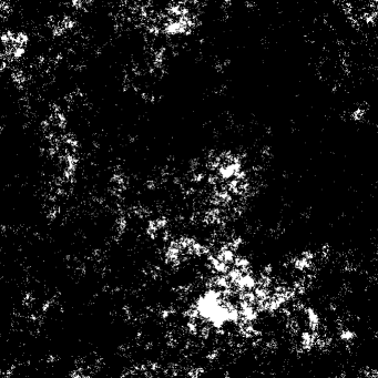
Figure 1: Simulation of $W[0,t]$ (shown in black) for $t=15$ in $d=2$. The holes in $\mathbb{T}^{2}\setminus W[0,t]$ (shown in white) have an irregular shape. The goal is to understand the geometry of the largest holes. The present paper only deals with $d\geq 3$. In Section 1.6.8 below we will reflect on what happens in $d=2$.

Regions with a random boundary have been studied intensively in the literature, and questions such as Question 1 have been approached from a variety of perspectives. Sznitman S1998 studies the principal Dirichlet eigenvalue when a Poisson cloud of obstacles is removed from Euclidean space $\mathbb{R}^{d}$, $d\geq 1$. Van den Berg, Bolthausen and den Hollander vdBBdH2001 consider the large deviation properties of the volume of a Wiener sausage on $\mathbb{R}^{d}$, $d\geq 2$, and identify the geometric strategies for achieving these large deviations. Probabilistic techniques also play a role in the analysis of deterministic shapes, such as strong circularity in rotor-router and sandpile models shown by Levine and Peres LP2009 , and heat flow in the von Koch snowflake and its relatives analysed by van den Berg and den Hollander vdBdH1999 , van den Berg vdB2000 , and van den Berg and Bolthausen vdBB2004 . The discrete analogue to Question 1, random walk on a large discrete torus, is connected to the random interlacements model of Sznitman S2010 (to which we will return in Section 1.6.3 below).

Question 1 is studied by Dembo, Peres and Rosen DPR2003 for $d\geq 3$ and Dembo, Peres, Rosen and Zeitouni DPRZ2004 for $d=2$. In both cases, a law of large numbers is established for the $\epsilon$-cover time (the time for the Brownian motion to come within distance $\epsilon$ of every point) as $\epsilon\downarrow 0$. For $d\geq 3$, Dembo, Peres and Rosen also obtain the multifractal spectrum of late points (those points that are approached within distance $\epsilon$ on a time scale that is a positive fraction of the $\epsilon$-cover time). In the present paper we will consider a large but fixed time $t$, and we will use a key lemma from DPR2003 to obtain global information about $\mathbb{T}^{d}\setminus W[0,t]$. Throughout the paper we fix a dimension $d\geq 3$. The behaviour in $d=2$ is expected to be quite different (see the discussion in Section 1.6.8 below).

A random set is an infinite-dimensional object, hence issues of measurability require care. In general, events are defined in terms of whether a random closed set intersects a given closed set, or whether a random open set contains a given closed set: see Matheron M1975 or Molchanov M2005 for a general theory of random sets and questions related to their geometry. On the torus we will parametrize these basic events as

$$\left\{(x+\varphi E)\cap W[0,t]=\varnothing\right\}=\{x+\varphi E\subset\mathbb{T}^{d}\setminus W[0,t]\},\qquad x\in\mathbb{T}^{d},\,E\subset\mathbb{R}^{d}\text{ compact}$$ (1.1)

(see (1.6) below), where $\varphi>0$ acts as a scaling factor. The set $E$ in (1.1) plays a role similar to that of a test function, and we will restrict our attention to suitably regular sets $E$, for instance, compact sets with non-empty interior.

$\bullet$ In giving an answer to Question 1, we must distinguish between global properties, such as the size of the largest inradius or the principal Dirichlet eigenvalue of the random set, and local properties, such as whether or not the random set is locally connected. In the present paper we focus on the global properties of $\mathbb{T}^{d}\setminus W[0,t]$. We will therefore be interested in the existence of subsets of $\mathbb{T}^{d}\setminus W[0,t]$ of a given form:

Question 2

For a given compact set $E\subset\mathbb{R}^{d}$, what is the probability of the event

$$\left\{\exists x\in\mathbb{T}^{d}\colon\,x+\varphi E\subset\mathbb{T}^{d}\setminus W[0,t]\right\}=\bigcup_{x\in\mathbb{T}^{d}}\left\{x+\varphi E\subset\mathbb{T}^{d}\setminus W[0,t]\right\}$$ (1.2)

formed as the uncountable union of events from (1.1)?

For instance, questions about the inradius can be formulated in terms of Question 2 by setting $E$ to be a ball.

The answer to Question 2 depends on the scaling factor $\varphi$. To obtain a non-trivial result we are led to choose $\varphi=\varphi_{d}(t)$ depending on time, where

$$\varphi_{d}(t)=\left(\frac{d}{(d-2)\kappa_{d}}\,\frac{\log t}{t}\right)^{1/(d-2)},\qquad t>1,$$ (1.3)

and $\kappa_{d}$ is the constant

$$\kappa_{d}=\frac{2\pi^{d/2}}{\Gamma(d/2-1)}.$$ (1.4)

We will see that $\varphi_{d}(t)$ represents the linear size of the largest subsets of $\mathbb{T}^{d}\setminus W[0,t]$, in the sense that the limiting probability of the event in (1.2) decreases from $1$ to $0$ as the set $E$ increases from small to large, in the sense of small or large capacity (see Section 1.3.3 below).

In what follows we will see that $T^{d}\setminus W[0,t]$ is controlled by two spatial scales:

$$\varphi_{\mathrm{local}}(t)=\left(\frac{1}{t}\right)^{1/(d-2)},\qquad\varphi_{\mathrm{global}}(t)=\left(\frac{\log t}{t}\right)^{1/(d-2)}.$$ (1.5)

The linear size of the typical holes in $T^{d}\setminus W[0,t]$ is of order $\varphi_{\mathrm{local}}(t)$, the linear size of the largest holes of order $\varphi_{\mathrm{global}}(t)$. The choice (1.3) of $\varphi_{d}(t)$ is a fine tuning of the latter.

$\bullet$ For a typical point $x\in\mathbb{T}^{d}$, the event $\left\{x+\varphi_{d}(t)E\subset\mathbb{T}^{d}\setminus W[0,t]\right\}$ in (1.1) is unlikely to occur even when $E$ is small. However, given a compact set $E\subset\mathbb{R}^{d}$, the points $x\in\mathbb{T}^{d}$ for which $x+\varphi_{d}(t)E\subset\mathbb{T}^{d}\setminus W[0,t]$ (i.e., the points that realize the event in (1.2)) are atypical, and we can ask whether the subset $x+\varphi_{d}(t)E$ is likely to form part of a considerably larger subset:

Question 3

Are the points $x\in\mathbb{T}^{d}$ for which $x+\varphi_{d}(t)E\subset\mathbb{T}^{d}\setminus W[0,t]$ likely to satisfy $x+\varphi_{d}(t)E^{\prime}\subset\mathbb{T}^{d}\setminus W[0,t]$ for some substantially larger set $E^{\prime}\supset E$?

Question 3 aims to distinguish between the two qualitative pictures shown in Fig. 2, which we call sparse and dense, respectively. We will show that in $d\geq 3$ the answer to Question 3 is no, i.e., the picture is dense as in part (b) of Fig. 2. In Section 1.6.8 below we will argue that in $d=2$ the answer to Question 3 is yes, i.e., the picture is sparse as in part (a) of Fig. 2. This can already be seen from Fig. 1.

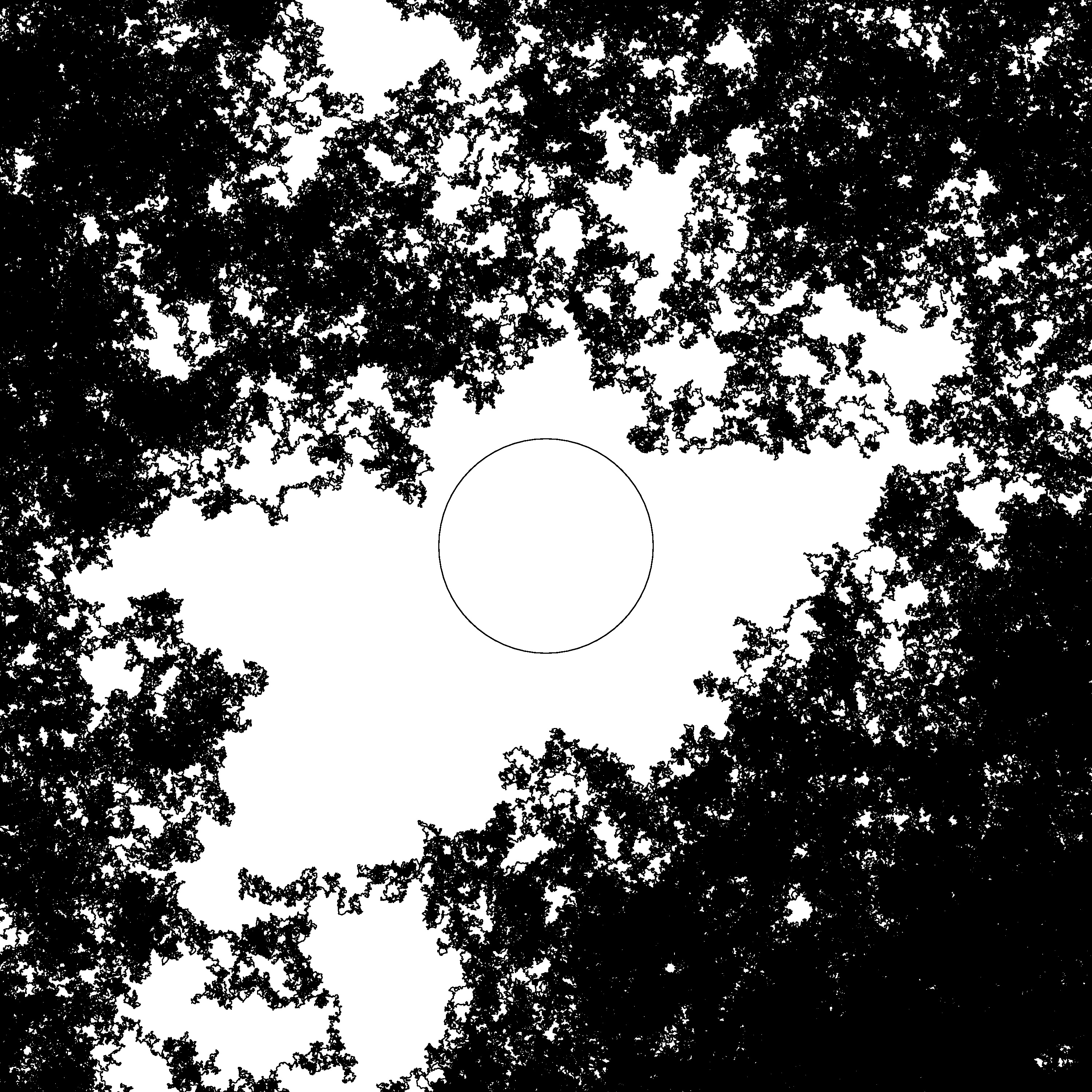
(a) (b)

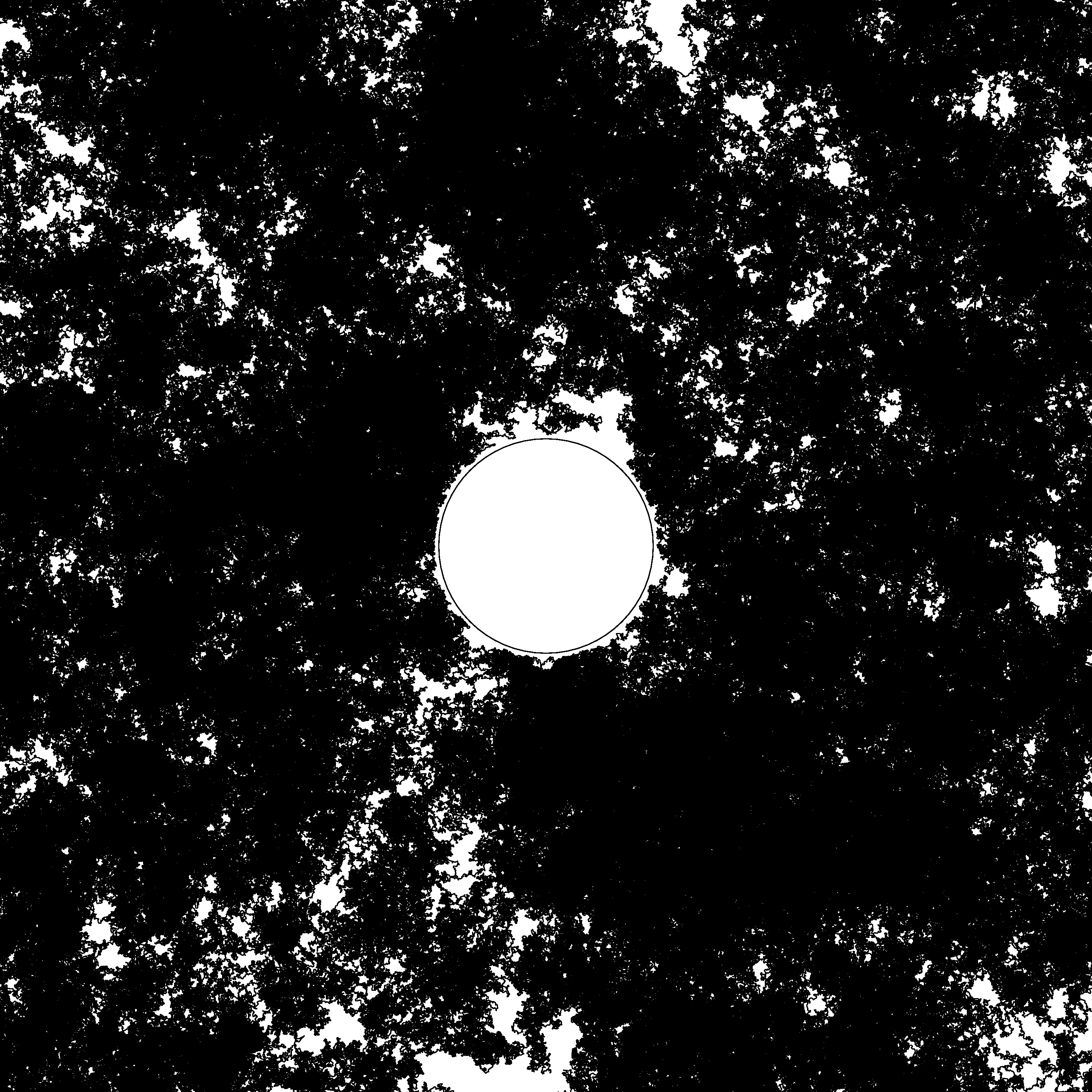
Figure 2: The vicinity of $x+\varphi_{d}(t)E\subset\mathbb{T}^{d}\setminus W[0,t]$. The circular region in part (a) can be enlarged substantially while remaining a subset of $\mathbb{T}^{d}\setminus W[0,t]$, the circular region in part (b) cannot.

In a similar spirit, we can ask about temporal versus spatial avoidance strategies:

Question 4

For a given $x\in\mathbb{T}^{d}$, does the unlikely event $\left\{x+\varphi_{d}(t)E\subset\mathbb{T}^{d}\setminus W[0,t]\right\}$ arise primarily because the Brownian motion spends an unusually small amount of time near $x$, or because the Brownian motion spends a typical amount of time near $x$ and simply happens to avoid the set $x+\varphi_{d}(t)E$?

Questions 3 and 4, though not equivalent, are interrelated: if the Brownian motion spends an unusually small amount of time near $x$, then it may be plausibly expected to fill the vicinity of $x$ less densely, and vice versa. We will show that in $d\geq 3$ the Brownian motion follows a spatial avoidance strategy (the second alternative in Question 4) and that, indeed, the Brownian motion is very likely to spend approximately the same amount of time around all points of $\mathbb{T}^{d}$. In Section 1.6.8 below we will argue that in $d=2$ the first alternative in Question 4 applies.

$\bullet$ The negative answer to Question 3 and the heuristic picture in Fig. 2(b) suggest that regions of $\mathbb{T}^{d}$ where $W[0,t]$ is relatively dense nearly separate the large subsets $x+\varphi_{d}(t)E\subset\mathbb{T}^{d}\setminus W[0,t]$ into disjoint components. Making sense of this heuristic is complicated by the fact that $\mathbb{T}^{d}\setminus W[0,t]$ is connected almost surely (see Proposition 2 below), so that all large subsets belong to the same connected component in $\mathbb{T}^{d}\setminus W[0,t]$.

Question 5

Can the approximate component structure of the large subsets of $\mathbb{T}^{d}\setminus W[0,t]$ be captured in a well-defined way?

We will provide a positive answer to Question 5 by enlarging the Brownian path $W[0,t]$ to a Wiener sausage $W_{\rho(t)}[0,t]$ of radius $\rho(t)=o(\varphi_{d}(t))$. Under suitable hypotheses on the enlargement radius $\rho(t)$ (see (1.17) below) we are able to control certain properties of all the connected components of $\mathbb{T}^{d}\setminus W_{\rho(t)}[0,t]$ simultaneously: for instance, we compute the asymptotics of their maximum possible volume and capacity and minimal possible Dirichlet eigenvalue. The well-definedness of the approximate component structure lies in the fact that (subject to the hypothesis in (1.17) below) these properties do not depend on the precise choice of $\rho(t)$.

The existence of a connected component of $\mathbb{T}^{d}\setminus W_{\rho(t)}[0,t]$ having a given property, for instance, having at least a specified volume, involves an uncountable union of the events in (1.2) as $E$ runs over a suitable class of connected sets. Central to our arguments is a discretization procedure that reduces such an uncountable union to a suitably controlled finite union (see Section 3 below).

1.2 Outline

Our main results concern the extremal geometry of the set $\mathbb{T}^{d}\setminus W[0,t]$ as $t\to\infty$. Our key theorem is a large deviation estimate for the shape of the component with largest capacity in $\mathbb{T}^{d}\setminus W_{\rho(t)}[0,t]$ as $t\to\infty$, where $W_{\rho(t)}[0,t]$ is the Wiener sausage of radius $\rho(t)$. From this we derive large deviation principles for the maximal volume and the principal Dirichlet eigenvalue of the components of $\mathbb{T}^{d}\setminus W_{\rho(t)}[0,t]$ as $t\to\infty$, and identify the number of disjoint translates of $\varphi_{d}(t)E$ in $\mathbb{T}^{d}\setminus W[0,t]$ as $t\to\infty$ for suitable sets $E$. We further derive large deviation principles for the largest inradius as $t\to\infty$ and the $\epsilon$-cover time as $\epsilon\downarrow 0$, extending laws of large numbers that were derived in Dembo, Peres and Rosen DPR2003 . Along the way we settle the five questions raised in Section 1.1.

It turns out that the costs of the various large deviations are asymmetric: polynomial in one direction and stretched exponential in the other direction. Our main results are linked by the heuristic that sets of the form $x+\varphi_{d}(t)E$ appear according to a Poisson point process with total intensity $t^{J_{d}(\operatorname{Cap}E)+o(1)}$, where $J_{d}$ is given by (1.16) below (see Fig. 3 below).

The remainder of the paper is organised as follows. In Section 1.3 we give definitions and introduce notations. In Sections 1.4 and 1.5 we state our main results: four theorems, five corollaries and two propositions. In Section 1.6 we discuss these results, state some conjectures, make the link with random interlacements, and reflect on what happens in $d=2$. Section 2 contains various estimates on hitting times, hitting numbers and hitting probabilities for Brownian excursions between the boundaries of concentric balls, which serve as key ingredients in the proofs of the main results. Section 3 looks at non-intersection probabilities for lattice animals, which serve as discrete approximations to continuum sets. The proofs of the main results are given in Sections 4–5. Appendix A contains the proof of two lemmas that are used along the way.

1.3 Definitions and notations

1.3.1 Torus

The $d$-dimensional unit torus $\mathbb{T}^{d}$ is the quotient space $\mathbb{R}^{d}/\mathbb{Z}^{d}$, with the canonical projection map $\pi_{0}\colon\,\mathbb{R}^{d}\to\mathbb{T}^{d}$. We consider $\mathbb{T}^{d}$ as a Riemannian manifold in such a way that $\pi_{0}$ is a local isometry. The space $\mathbb{R}^{d}$ acts on $\mathbb{T}^{d}$ by translation: given $x=\pi_{0}(y_{0})\in\mathbb{T}^{d},y_{0},y\in\mathbb{R}^{d}$, we define $x+y=\pi_{0}(y_{0}+y)\in\mathbb{T}^{d}$. (Having made this definition, we will no longer need to refer to the projection map $\pi_{0}$, nor to the particular representation of the torus $\mathbb{T}^{d}$.) Given a set $E\subset\mathbb{R}^{d}$, a scale factor $\varphi>0$, and a point $x\in\mathbb{T}^{d}$ or $x\in\mathbb{R}^{d}$, we can now define

$$x+\varphi E=\left\{x+\varphi y\colon\,y\in E\right\}.$$ (1.6)

Euclidean distance in $\mathbb{R}^{d}$ and the induced distance in $\mathbb{T}^{d}$ are both denoted by $d(\cdot,\cdot)$. The distance from a point $x$ to a set $E$ is $d(x,E)=\inf\left\{d(x,y)\colon\,y\in E\right\}$. The closed ball of radius $r$ around a point $x$ is denoted by $B(x,r)$, for $x\in\mathbb{T}^{d}$ or $x\in\mathbb{R}^{d}$. We will only be concerned with the case $0<r<\tfrac{1}{2}$, so that $B(x,r)=x+B(0,r)$ for $x\in\mathbb{T}^{d}$ and the local isometry $B(0,r)\to B(x,r)$, $y\mapsto x+y$, is one-to-one.

1.3.2 Brownian motion and Wiener sausage

We write $\mathbb{P}_{x_{0}}$ for the law of the Brownian motion $W=(W(t))_{t\geq 0}$ on $\mathbb{T}^{d}$ started at $x_{0}\in\mathbb{T}^{d}$, i.e., the Markov process with generator $-\tfrac{1}{2}\Delta_{\mathbb{T}^{d}}$, where $\Delta_{\mathbb{T}^{d}}$ is the Laplace operator for $\mathbb{T}^{d}$. We can always take $W(t)=x_{0}+\tilde{W}(t)$, where $\tilde{W}=(\tilde{W}(t))_{t\geq 0}$ is the standard Brownian motion on $\mathbb{R}^{d}$ started at $0$, so that $W$ is the projection onto $\mathbb{T}^{d}$ (via $\pi_{0}$) of a Brownian motion in $\mathbb{R}^{d}$. When $x_{0}\in\mathbb{R}^{d}$ we will also use $\mathbb{P}_{x_{0}}$ for the law of the Brownian motion on $\mathbb{R}^{d}$. When the initial point $x_{0}$ is irrelevant we will write $\mathbb{P}$ instead of $\mathbb{P}_{x_{0}}$. The image of the Brownian motion over the time interval $[a,b]$ is denoted by $W[a,b]=\left\{W(s)\colon\,a\leq s\leq b\right\}$.

For $r>0$ and $E\subset\mathbb{R}^{d}$ or $E\subset\mathbb{T}^{d}$, we write $E_{r}=\cup_{x\in E}B(x,r)$ and $E_{-r}=[\cup_{x\in E^{c}}B(x,r)]^{c}$. The Wiener sausage of radius $r$ run for time $t$ is the $r$-enlargement of $W[0,t]$, i.e., $W_{r}[0,t]=\cup_{s\in[0,t]}B(W(s),r)$.

1.3.3 Capacity

The (Newtonian) capacity of a Borel set $E\subset\mathbb{R}^{d}$, denoted by $\operatorname{Cap}E$, can be defined as

$$\operatorname{Cap}E=\left(\inf_{\mu\in\mathcal{P}(E)}\iint_{E\times E}G(x,y)\,d\mu(x)\,d\mu(y)\right)^{-1},$$ (1.7)

where the infimum runs over the set of probability measures $\mu$ on $E$, and

$$G(x,y)=\frac{\Gamma(d/2-1)}{2\pi^{d/2}d(x,y)^{d-2}}$$ (1.8)

is the Green function associated with Brownian motion on $\mathbb{R}^{d}$ (throughout the paper we restrict to $d\geq 3$). In terms of the constant $\kappa_{d}$ from (1.4), we can write $G(x,y)=1/\kappa_{d}\,d(x,y)^{d-2}$, and it emerges that $\kappa_{d}=\operatorname{Cap}B(0,1)$ is the capacity of the unit ball.

The function $E\mapsto\operatorname{Cap}E$ is non-decreasing in $E$ and satisfies the scaling relation

$$\operatorname{Cap}(\varphi E)=\varphi^{d-2}\operatorname{Cap}E,\qquad\varphi>0,$$ (1.9)

and the union bound

$$\operatorname{Cap}(E\cup E^{\prime})+\operatorname{Cap}(E\cap E^{\prime})\leq\operatorname{Cap}E+\operatorname{Cap}E^{\prime}.$$ (1.10)

Capacity has an interpretation in terms of Brownian hitting probabilities:

$$\lim_{d(x,0)\to\infty}d(x,0)^{d-2}\,\mathbb{P}_{x}\big{(}W\left[0,\infty\right)\cap E\neq\varnothing\big{)}=\frac{\operatorname{Cap}E}{\kappa_{d}},\qquad E\subset\mathbb{R}^{d}\text{ bounded Borel.}$$ (1.11)

Thus, capacity measures how likely it is for a set to be hit by a Brownian motion that starts far away. We will make extensive use of asymptotic properties similar to (1.11).

If a set $E$ is polar – i.e., with probability 1, $E$ is not hit by a Brownian motion started away from $E$ – then $\operatorname{Cap}E=0$. For instance, any finite or countable union of $(d-2)$-dimensional subspaces has capacity zero.

1.3.4 Sets

The boundary of a set $E$ is denoted by $\partial E$, the interior by ${\rm int}\!\left(E\right)$, and the closure by ${\rm clo}\!\left(E\right)$. We define

$$\mathcal{E}_{c}=\left\{\text{$E\subset\mathbb{R}^{d}$ compact: $E$ and $\mathbb{R}^{d}\setminus E$ connected}\right\}$$ (1.12)

We will use these sets to describe the possible components of $\mathbb{T}^{d}\setminus W_{\rho(t)}[0,t]$. We further define

$$\mathcal{E}^{*}=\left\{\text{$E\subset\mathbb{R}^{d}$ compact: $\operatorname{Cap}E=\operatorname{Cap}({\rm int}\!\left(E\right))$}\right\}\cup\left\{\text{$E\subset\mathbb{R}^{d}$ bounded open: $\operatorname{Cap}E=\operatorname{Cap}({\rm clo}\!\left(E\right))$}\right\}.$$ (1.13)

The condition $\operatorname{Cap}({\rm int}\!\left(E\right))=\operatorname{Cap}({\rm clo}\!\left(E\right))$ in the definition of $\mathcal{E}^{*}$ is satisfied when every point of $\partial E$ is a regular point for ${\rm int}\!\left(E\right)$, which in turn is satisfied when $E$ satisfies a cone condition at every point (see Port and Stone (PS1978, , Chapter 2, Proposition 3.3)). In particular, any finite union of cubes, or any $r$-enlargement $E_{r}$ with $r>0$ of a compact set $E$, belongs to $\mathcal{E}^{*}$.

1.3.5 Maximal capacity of a component

A central role will be played by the largest capacity $\kappa^{*}(t,\rho)$ for a component of $\mathbb{T}^{d}\setminus W_{\rho}[0,t]$, defined by

$$\kappa^{*}(t,\rho)=\sup\left\{\operatorname{Cap}E\colon\,\text{$E\subset\mathbb{R}^{d}$ connected, $x+E\subset\mathbb{T}^{d}\setminus W_{\rho}[0,t]$ for some $x\in\mathbb{T}^{d}$}\right\}.$$ (1.14)

Note that by rescaling we have

$$\frac{\kappa^{*}(t,\rho)}{\varphi_{d}(t)^{d-2}}=\sup\left\{\operatorname{Cap}E\colon\,\text{$E\subset\mathbb{R}^{d}$ connected, $x+\varphi_{d}(t)E\subset\mathbb{T}^{d}\setminus W_{\rho}[0,t]$ for some $x\in\mathbb{T}^{d}$}\right\}.$$ (1.15)

1.4 Component structure

We begin by describing the component structure of $\mathbb{T}^{d}\setminus W_{\rho}[0,t]$. In formulating the results below we will use the abbreviation (see Fig. 3(a))

$$J_{d}(\kappa)=\frac{d}{d-2}\left(1-\frac{\kappa}{\kappa_{d}}\right),\qquad\kappa\geq 0.$$ (1.16)

(a) (b)

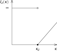
Figure 3: (a) The function $\kappa\mapsto J_{d}(\kappa)$ in (1.16). (b) The rate function $\kappa\mapsto I_{d}(\kappa)$ in (1.18).

Our first theorem quantifies the likelihood of finding sets of large capacity that do not intersect $W_{\rho}[0,t]$, for $\rho$ in a certain window between the local and the global spatial scales defined in (1.5).

Theorem 1.1

Fix a positive function $t\mapsto\rho(t)$ satisfying

$$\lim_{t\to\infty}\frac{\rho(t)}{\varphi_{d}(t)}=0,\qquad\lim_{t\to\infty}\frac{(\log t)^{1/d}\rho(t)}{\varphi_{d}(t)}=\infty.$$ (1.17)

Then the family $\mathbb{P}(\kappa^{*}(t,\rho)/\varphi_{d}(t)^{d-2}\in\cdot)$, $t>1$, satisfies the LDP on $[0,\infty]$ with rate $\log t$ and rate function (see Fig. 3(b))

$$I_{d}(\kappa)=\begin{cases}-J_{d}(\kappa),&\kappa\geq\kappa_{d},\\ \infty,&\kappa<\kappa_{d},\end{cases}$$ (1.18)

with the convention that $I_{d}(\infty)=\infty$.

The counterpart of Theorem 1.1 for small capacities is contained in the following two theorems, which show that components of small capacity are likely to exist and to be numerous. Let $\chi_{\rho}(t,\kappa)$ denote the number of components $C$ of $\mathbb{T}^{d}\setminus W_{\rho}[0,t]$ such that $C$ contains some ball of radius $\rho$ and has the form $C=x+\varphi_{d}(t)E$ for a connected open set $E$ with $\operatorname{Cap}E\geq\kappa$.

Theorem 1.2

Fix a positive function $t\mapsto\rho(t)$ satisfying (1.17), and let $\kappa<\kappa_{d}$. Then

$$\lim_{t\to\infty}\frac{\log\chi_{\rho(t)}(t,\kappa)}{\log t}=J_{d}(\kappa)\qquad\text{in $\mathbb{P}$-probability.}$$ (1.19)

Theorem 1.3

Fix a non-negative function $t\mapsto\rho(t)$ satisfying $\rho(t)=o(\varphi_{d}(t))$, and let $E\subset\mathbb{R}^{d}$ be compact with $\operatorname{Cap}E<\kappa_{d}$. Then

$$\log\mathbb{P}\left(\nexists\,x\in\mathbb{T}^{d}\colon\,x+\varphi_{d}(t)E\subset\mathbb{T}^{d}\setminus W_{\rho(t)}[0,t]\right)\leq-t^{J_{d}(\operatorname{Cap}E)+o(1)},\qquad t\to\infty.$$ (1.20)

The next theorem identifies the shape of the components of $\mathbb{T}^{d}\setminus W_{\rho(t)}[0,t]$. For $E\subset E^{\prime}$ a pair of nested compact connected subsets of $\mathbb{R}^{d}$, we say that a component $C$ of $\mathbb{T}^{d}\setminus W_{\rho}[0,t]$ satisfies condition ($\mathcal{C}(t,\rho,E,E^{\prime})$) when

$$C=x+\varphi_{d}(t)U,\qquad x\in\mathbb{T}^{d},\,E\subset U\subset E^{\prime}. \mathcal{C}(t,\rho,E,E^{\prime})$$ ()

Define $\chi_{\rho}(t,E,E^{\prime})$ to be the number of components of $\mathbb{T}^{d}\setminus W_{\rho}[0,t]$ satisfying condition ($\mathcal{C}(t,\rho,E,E^{\prime})$), and define $F_{\rho}(t,E,E^{\prime})$ to be the event

$$F_{\rho}(t,E,E^{\prime})=\left\{\parbox{275.0pt}{There exists a component $C=x+\varphi_{d}(t)U$ of $\mathbb{T}^{d}\setminus W_{\rho}[0,t]$ satisfying condition \eqref{CtrhoEEprime}, and any other component $C^{\prime}=x^{\prime}+\varphi_{d}(t)U^{\prime}$ has $\operatorname{Cap}U^{\prime}<\operatorname{Cap}U$.}\right\}$$ (1.21)

In words, $F_{\rho}(t,E,E^{\prime})$ is the event that $\mathbb{T}^{d}\setminus W_{\rho}[0,t]$ contains a component sandwiched between $x+\varphi_{d}(t)E$ and $x+\varphi_{d}(t)E^{\prime}$, and any other component has smaller capacity (when viewed as a subset of $\mathbb{R}^{d}$).

Theorem 1.4

Fix a positive function $t\mapsto\rho(t)$ satisfying (1.17), let $E\in\mathcal{E}_{c}$, and let $\delta>0$. If $\operatorname{Cap}E\geq\kappa_{d}$, then

$$\lim_{t\to\infty}\frac{\log\mathbb{P}\bigl{(}F_{\rho(t)}(t,E,E_{\delta})\bigr{)}}{\log t}=J_{d}(\operatorname{Cap}E)\quad(=-I_{d}(\operatorname{Cap}E)),$$ (1.22)

while if $\operatorname{Cap}E<\kappa_{d}$, then

$$\lim_{t\to\infty}\frac{\log\chi_{\rho(t)}(t,E,E_{\delta})}{\log t}=J_{d}(\operatorname{Cap}E)\qquad\text{in $\mathbb{P}$-probability.}$$ (1.23)

Theorems 1.1–1.4 yield the following corollary. For $E\subset\mathbb{R}^{d}$, let $\chi(t,E)$ denote the maximal number of disjoint translates $x+\varphi_{d}(t)E$ in $\mathbb{T}^{d}\setminus W[0,t]$.

Corollary 1

Suppose that $E\in\mathcal{E}^{*}$. Then

$$\lim_{t\to\infty}\mathbb{P}\left(\exists\,x\in\mathbb{T}^{d}\colon\,x+\varphi_{d}(t)E\subset\mathbb{T}^{d}\setminus W[0,t]\right)=\begin{cases}1,&\operatorname{Cap}E<\kappa_{d},\\ 0,&\operatorname{Cap}E>\kappa_{d}.\end{cases}$$ (1.24)

Furthermore,

$$\lim_{t\to\infty}\frac{\log\mathbb{P}(\exists\,x\in\mathbb{T}^{d}\colon\,x+\varphi_{d}(t)E\subset\mathbb{T}^{d}\setminus W[0,t])}{\log t}=J_{d}(\operatorname{Cap}E)\vee 0,$$ (1.25)

and if $\operatorname{Cap}E<\kappa_{d}$, then

$$\lim_{t\to\infty}\frac{\log\chi(t,E)}{\log t}=J_{d}(\operatorname{Cap}E)\quad\text{in $\mathbb{P}$-probability.}$$ (1.26)

1.5 Geometric structure

Having described the components in terms of their capacities in Section 1.4, we are ready to look at the geometric structure of our random set. Our first corollary concerns the maximal volume of a component of $\mathbb{T}^{d}\setminus W_{\rho}[0,t]$, which we denote by $V(t,\rho)$. Volume is taken w.r.t. the $d$-dimensional Lebesgue measure, and we write $V_{d}=\operatorname{Vol}B(0,1)$ for the volume of the $d$-dimensional unit ball.

Corollary 2

Subject to (1.17), the family $\mathbb{P}(V(t,\rho(t))/\varphi_{d}(t)^{d}\in\cdot)$, $t>1$, satisfies the LDP on $(0,\infty)$ with rate $\log t$ and rate function

$$I^{\rm volume}_{d}(v)=I_{d}\left(\kappa_{d}(v/V_{d})^{(d-2)/d}\right)\!.$$ (1.27)

Moreover, for $v<V_{d}$,

$$\log\mathbb{P}\big{(}V(t,\rho(t))/\varphi_{d}(t)^{d}<v\big{)}\leq-t^{J_{d}(\kappa_{d}(v/V_{d})^{(d-2)/d})+o(1)},\qquad t\to\infty.$$ (1.28)

Our second corollary concerns $\lambda(t,\rho)=\lambda(\mathbb{T}^{d}\setminus W_{\rho}[0,t])$, the principal Dirichlet eigenvalue of $\mathbb{T}^{d}\setminus W_{\rho}[0,t]$, where by $\lambda(E)$ (for $E\subset\mathbb{T}^{d}$ or $E\subset\mathbb{R}^{d}$) we mean the principal eigenvalue of the operator $-\tfrac{1}{2}\Delta_{E}$ with Dirichlet boundary conditions on $\partial E$. We write $\lambda_{d}=\lambda(B(0,1))$ for the principal Dirichlet eigenvalue of the $d$-dimensional unit ball.

Corollary 3

Subject to (1.17), the family $\mathbb{P}(\varphi_{d}(t)^{2}\lambda(t,\rho(t))\in\cdot)$, $t>1$, satisfies the LDP on $(0,\infty)$ with rate $\log t$ and rate function

$$I^{\rm Dirichlet}_{d}(\lambda)=I_{d}\left(\kappa_{d}(\lambda_{d}/\lambda)^{(d-2)/2}\right)\!.$$ (1.29)

Moreover, for $\lambda>\lambda_{d}$,

$$\log\mathbb{P}\big{(}\varphi_{d}(t)^{2}\lambda(t,\rho(t))\geq\lambda\big{)}\leq-t^{J_{d}(\kappa_{d}(\lambda_{d}/\lambda)^{(d-2)/2})+o(1)},\qquad t\to\infty.$$ (1.30)

Our last two corollaries concern the largest inradius of $\mathbb{T}^{d}\setminus W[0,t]$,

$$\rho_{\rm in}(t)=\sup_{x\in\mathbb{T}^{d}}d(x,W[0,t])=\sup\left\{\rho\geq 0\colon\,\mathbb{T}^{d}\setminus W_{\rho}[0,t]\neq\varnothing\right\},\qquad t>0,$$ (1.31)

and the $\epsilon$-cover time,

$$\mathcal{C}_{\epsilon}=\sup_{x\in\mathbb{T}^{d}}\inf\left\{\big{.}t\geq 0\colon\,d(x,W[0,t])\leq\epsilon\right\}=\inf\left\{\big{.}t\geq 0\colon\,\rho_{\rm in}(t)\leq\epsilon\right\},\qquad 0<\epsilon<1.$$ (1.32)

For the latter we need the scaling function

$$\psi_{d}(\epsilon)=\frac{\epsilon^{-(d-2)}\log(1/\epsilon)}{\kappa_{d}},\qquad 0<\epsilon<1.$$ (1.33)

Corollary 4

The family $\mathbb{P}(\rho_{\rm in}(t)/\varphi_{d}(t)\in\cdot\,)$, $t>1$, satisfies the LDP on $(0,\infty)$ with rate $\log t$ and rate function

$$I^{\rm inradius}_{d}(r)=I_{d}(\kappa_{d}\,r^{d-2}).$$ (1.34)

Moreover, for $0<r<1$,

$$\log\mathbb{P}\big{(}\rho_{\rm in}(t)/\varphi_{d}(t)<r\big{)}\leq-t^{J_{d}(\kappa_{d}\,r^{d-2})+o(1)},\qquad t\to\infty.$$ (1.35)

Corollary 5

The family $\mathbb{P}(\mathcal{C}_{\epsilon}/\psi_{d}(\epsilon)\in\cdot\,)$, $0<\epsilon<1$, satisfies the LDP on $(0,\infty)$ with rate $\log(1/\epsilon)$ and rate function

$$I_{d}^{\rm cover}(u)=\begin{cases}u-d,&u\geq d,\\ \infty,&0<u<d.\end{cases}$$ (1.36)

Moreover, for $0<u<d$,

$$\log\mathbb{P}\big{(}\mathcal{C}_{\epsilon}/\psi_{d}(\epsilon)<u\big{)}\leq-\epsilon^{-(d-u)+o(1)},\qquad\epsilon\downarrow 0.$$ (1.37)

Corollary 5 is equivalent to Corollary 4 because of the relation $\left\{\rho_{\rm in}(t)>\epsilon\right\}=\left\{\mathcal{C}_{\epsilon}>t\right\}$ and the asymptotics

$$\varphi_{d}(u\psi_{d}(\epsilon))\sim\left(\frac{u}{d}\right)^{1/(d-2)}\epsilon,\quad\epsilon\downarrow 0,\,u>0,\qquad\psi_{d}(r\varphi_{d}(t))\sim\frac{t}{dr^{d-2}},\quad t\to\infty,\,r>0.$$ (1.38)

1.6 Discussion

1.6.1 Upward versus downward deviations and the role of $J_{d}(\kappa)$

Theorem 1.1 says that the region with largest capacity not intersecting the Wiener sausage of radius $\rho(t)$ lives on scale $\varphi_{d}(t)$, and that upward large deviations on this scale have a cost that decays polynomially in $t$. Theorem 1.2 identifies how many components there are with small capacity. This number grows polynomially in $t$. Theorem 1.3 says that this number is extremely unlikely to be zero: the cost is stretched exponential in $t$. Theorem 1.4 completes the picture obtained from Theorems 1.1–1.3 by showing that components can approximate any shape in $\mathcal{E}_{c}$.

Theorems 1.1–1.4 and are linked by the heuristic that components of the form $x+\varphi_{d}(t)E$ appear according to a Poisson point process with total intensity $t^{J_{d}(\operatorname{Cap}E)+o(1)}$. When $\operatorname{Cap}E>\kappa_{d}$ we have $J_{d}(\operatorname{Cap}E)<0$, and the likelihood of even a single such component is $t^{-\left|J_{d}(\operatorname{Cap}E)\right|+o(1)}$, as in Corollary 1. When $\operatorname{Cap}E<\kappa_{d}$ we have $J_{d}(\operatorname{Cap}E)>0$, and a Poisson random variable $X$ of mean $t^{J_{d}(\operatorname{Cap}E)+o(1)}$ satisfies $X=t^{J_{d}(\operatorname{Cap}E)+o(1)}$ with high probability and $\mathbb{P}(X=0)=\exp[-t^{J_{d}(\operatorname{Cap}E)+o(1)}]$. Based on this heuristic, we conjecture that the inequalities in (1.28), (1.30), (1.35) and (1.37) are all equalities asymptotically.

1.6.2 Components and the role of $\rho(t)$

Theorems 1.1–1.4 concern components of the form $x+\varphi_{d}(t)E$. We begin by remarking that, with high probability, all components have this form:

Proposition 1

Assume (1.17). Let ${\rm Wrap}(t,\rho)$ be the event that $\mathbb{T}^{d}\setminus W_{\rho}[0,t]$ has a component $C$ that, when considered as a Riemannian manifold with its intrinsic metric, is not the isometric image $x+E$ of some bounded subset $E$ of $\mathbb{R}^{d}$. Then

$$\lim_{t\to\infty}\frac{\log\mathbb{P}\left({\rm Wrap}(t,\rho(t))\right)}{\log t}=-\infty.$$ (1.39)

Informally, such a component must “wrap around” the torus, so that the local isometry from $\mathbb{R}^{d}$ to $\mathbb{T}^{d}$ is not a global isometry. Proposition 1 means that, apart from a negligible event, we may sensibly consider the components as subsets of $\mathbb{R}^{d}$ and discuss their capacities as defined in (1.7).

Collectively, Theorems 1.1–1.4, Corollaries 2–3 and Proposition 1 show that $\mathbb{T}^{d}\setminus W_{\rho(t)}[0,t]$ has a component structure, with well-defined bounds on the capacities, volumes and principal Dirichlet eigenvalues of these components. By contrast, the choice $\rho(t)=0$ does not give a component structure at all:

Proposition 2

With probability $1$, the set $\mathbb{T}^{d}\setminus W[0,t]$ is path-connected, open and dense for every $t$, and the set $\mathbb{T}^{d}\setminus W\left[0,\infty\right)$ is path-connected, locally path-connected and dense.

The picture behind Propositions 1–2 is that the set $\mathbb{T}^{d}\setminus W[0,t]$ consists of “lakes” whose linear size is of order $\varphi_{d}(t)$, connected by narrow “channels” whose linear size is at most $\varphi_{d}(t)/(\log t)^{1/d}$. By inflating the Brownian motion to a Wiener sausage of radius $\rho(t)$ with (recall (1.5) and (1.17))

$$\varphi_{\mathrm{local}}(t)\ll\varphi_{d}(t)/(\log t)^{1/d}\ll\rho(t)\ll\varphi_{d}(t)\asymp\varphi_{\mathrm{global}}(t),$$ (1.40)

we effectively block off these channels, so that $\mathbb{T}^{d}\setminus W_{\rho(t)}[0,t]$ consists of disjoint lakes.

Proposition 2 shows that some lower bound on $\rho(t)$ is necessary for the results of Theorems 1.1–1.4, Corollaries 2–3 and Proposition 1 to hold. It would be of interest to know whether the condition $\rho(t)\gg\varphi_{d}(t)/(\log t)^{1/d}$ can be relaxed, i.e., whether the true size of the channels is of smaller order than $\varphi_{d}(t)/(\log t)^{1/d}$. By analogy with the random interlacements model (see Section 1.6.3 below), the relevant regime to study would be $\varphi_{\mathrm{local}}(t)\asymp\varphi_{d}(t)/(\log t)^{1/(d-2)}\ll\rho(t)\ll\varphi_{d}(t)/(\log t)^{1/d}$, i.e., the missing part of (1.40).

1.6.3 A comparison with random interlacements

The discrete analogue of $\mathbb{T}^{d}\setminus W[0,t]$ is the complement $\mathbb{T}_{N}^{d}\setminus S[0,n]$ of the path of a random walk $S=(S(n))_{n\in\mathbb{N}_{0}}$ on a large discrete torus $\mathbb{T}_{N}^{d}=(\mathbb{Z}/N\mathbb{Z})^{d}$. The spatial scale being fixed by discretization, it is necessary to take $N\to\infty$ and $n\to\infty$ simultaneously, and the choice $n=uN^{d}$ for $u\in(0,\infty)$ has been extensively studied: see for instance Benjamini and Sznitman BenjSznit2008 , Sznitman S2010 and Sidoravicius and Sznitman SS2009 . Teixeira and Windisch TeixWind2011 prove that $S[0,uN^{d}]$, seen locally from a typical point, converges in law as $N\to\infty$, namely,

$$\lim_{N\to\infty}\mathbb{P}\left((X_{N}+E)\cap S[0,uN^{d}]=\varnothing\right)=e^{-u\operatorname{Cap}_{\mathbb{Z}^{d}}E},\qquad E\subset\mathbb{Z}^{d}\text{ finite},$$ (1.41)

where $X_{N}$ is drawn uniformly from $\mathbb{T}_{N}^{d}$, and $\operatorname{Cap}_{\mathbb{Z}^{d}}E$ is the discrete capacity. The right-hand side of (1.41) is the non-intersection probability

$$\mathbb{P}(E\cap\mathcal{I}^{u}=\varnothing)=e^{-u\operatorname{Cap}_{\mathbb{Z}^{d}}E}$$ (1.42)

for the random interlacements model with parameter $u$ introduced by Sznitman S2010 . The set $\mathcal{I}^{u}\subset\mathbb{Z}^{d}$ can be constructed as the union of a certain Poisson point process of random walk paths, with an intensity measure proportional to the parameter $u$. The random interlacements model has a critical value $u_{*}\in(0,\infty)$ such that $\mathbb{Z}^{d}\setminus\mathcal{I}^{u}$ has an unbounded component a.s. when $u<u_{*}$ and has only bounded components a.s. when $u>u_{*}$.

The continuous analogue of (1.41) is the probability of the event in (1.1) with the scaling factor $\varphi=\varphi_{\mathrm{local}}(t)=t^{-1/(d-2)}$ instead of $\varphi=\varphi_{d}(t)\asymp\varphi_{\mathrm{global}}(t)$. Our methods (see Propositions 3 and 4 below) yield

$$\lim_{t\to\infty}\left((X+t^{-1/(d-2)}E)\cap W[0,t]=\varnothing\right)=e^{-\operatorname{Cap}E},\qquad E\subset\mathbb{R}^{d}\text{ compact},$$ (1.43)

for $X$ drawn uniformly from $\mathbb{T}^{d}$, which implies that the random set $\mathbb{T}^{d}\setminus W[0,t]$, seen locally from a typical point, converges in law (see Molchanov (M2005, , Theorem 6.5) for a discussion of convergence in law for random sets) to a random closed set $\mathcal{I}$ uniquely characterized by its non-intersection probabilities

$$\mathbb{P}(E\cap\mathcal{I}=\varnothing)=e^{-\operatorname{Cap}E},\qquad E\subset\mathbb{R}^{d}\text{ compact}.$$ (1.44)

As with the discrete random interlacements $\mathcal{I}^{u}$, the limiting random set $\mathcal{I}$ can be constructed from a Poisson point process of Brownian motion paths (see Sznitman (SznitmanBrInt, , Section 2)).

Because of scale invariance, no parameter is needed in (1.43)–(1.44). Indeed, the continuous model corresponds to a rescaled limit of the discrete model when $(N,u)$ is replaced by $(kN,u/k^{d-2})$ and $k\to\infty$. In this rescaling the parameter $u$ tends to zero, and $\mathbb{Z}^{d}\setminus\mathcal{I}^{u}$ loses its finite component structure, which is in accordance with the connectedness result Proposition 2.

Inflating the Brownian motion to a Wiener sausage can be interpreted as reintroducing a kind of discretization. However, because of (1.17), the spatial scale $\rho(t)$ of this discretization is much larger than the spatial scale $\varphi_{\mathrm{local}}(t)=t^{-1/(d-2)}$ corresponding to (1.43) (cf. Section 1.6.2).

In the random interlacements model no sharp bound is currently known for the tail behaviour of the capacity of the component containing the origin. Recently, Popov and Teixeira PopovTeixeiraSoftLocal showed that for $d\geq 3$ the diameter of the component containing $0$ in $\mathbb{Z}^{d}\setminus\mathcal{I}^{u}$ has an exponential tail for $u$ sufficiently large (with a logarithmic correction in $d=3$). In particular, the largest diameter of a component in a box of volume $N^{d}$, $d\geq 4$, can grow at most as $\log N$, and therefore the largest capacity of a component can grow at most as $(\log N)^{d-2}$.

When this last bound is translated heuristically to our context, the corresponding assertion is that the maximal capacity of a component is at most of order $(\log t)^{d-2}/t$. By Theorem 1.1, this bound is very far from sharp for $d\geq 4$. It is tempting to conjecture that the capacity of the component containing $0$ in $\mathbb{Z}^{d}\setminus\mathcal{I}^{u}$ also has an exponential tail for $u$ sufficiently large. The reasonableness of this conjecture is related to whether or not the condition on $\rho(t)$ in (1.17) can be weakened to $\rho(t)\geq u\varphi_{\mathrm{local}}(t)$ for $u$ sufficiently large. Possibly the scaling behaviour of $\mathbb{T}^{d}\setminus W_{\rho(t)}[0,t]$ with $\rho(t)=u\varphi_{\mathrm{local}}(t)$ undergoes some sort of percolation transition at a critical value $\bar{u}_{*}\in(0,\infty)$.

1.6.4 Corollaries of the capacity bounds

Corollary 1 summarizes for which set $E$ a subset $x+\varphi_{d}(t)E\subset\mathbb{T}^{d}\setminus W[0,t]$ can be expected to exist: according to Theorems 1.1–1.4, subsets of large capacity are unlikely to exist, whereas subsets of small capacity are numerous.

Corollaries 2–3 follow from Theorems 1.1–1.4 with the help of the isoperimetric inequalities

$$\frac{\operatorname{Cap}E}{\kappa_{d}}\geq\left(\frac{\operatorname{Vol}E}{V_{d}}\right)^{(d-2)/d}\geq\left(\frac{\lambda_{d}}{\lambda(E)}\right)^{(d-2)/2},\qquad E\subset\mathbb{R}^{d}\text{ bounded open,}$$ (1.45)

where we recall that $\kappa_{d},V_{d},\lambda_{d}$ are the capacity, volume and principal Dirichlet eigenvalue of $B(0,1)$. The first inequality is the Poincaré-Faber-Szegö theorem, which says that among all sets with a given volume the ball has the smallest capacity. The second inequality is the Faber-Krahn theorem, which says that among all sets of a given volume the ball has the smallest Dirichlet eigenvalue. Comparing with Theorem 1.1, we see that the most efficient way to produce a component of a given large volume (or small principal Dirichlet eigenvalue) is for that component to be a ball.

Equality holds throughout (1.45) when $E$ is a ball, and the lower bounds in Corollaries 2–3, together with Corollaries 4–5, follow by specializing Theorems 1.1–1.4 to that case.

The large deviation principles in Theorem 1.1 and Corollaries 2–5 each imply a weak law of large numbers, e.g. $\lim_{t\to\infty}\kappa^{*}(t,\rho(t))/\varphi_{d}(t)^{d-2}=1$ in $\mathbb{P}$-probability. The weak laws of large numbers implied by Corollaries 4–5 were proved in Dembo, Peres and Rosen DPR2003 in the stronger form $\lim_{t\to\infty}\rho_{\rm in}(t)/\varphi_{d}(t)=1$ and $\lim_{t\to\infty}\mathcal{C}_{\epsilon}/\psi_{d}(\epsilon)=d$ $\mathbb{P}$-a.s. The $L^{1}$-version of this convergence is proved in van den Berg, Bolthausen and den Hollander vdBBdHpr . Note that none of these forms are equivalent: for instance, a.s. convergence does not follow from Corollaries 4–5, since the sum $\sum_{t\in\mathbb{N}}\exp[-I_{d}(\kappa)\log t]$ fails to converge when $I_{d}(\kappa)$ is small.

1.6.5 The maximal diameter of a component

There is no analogue of Corollary 2 for the maximal diameter instead of the maximal volume. The capacity and the diameter are related by $\operatorname{Cap}E\leq\kappa_{d}(\operatorname{diam}E)^{d-2}$. However, there is no inequality in the reverse direction: a set of fixed capacity can have an arbitrarily large diameter. It turns out that the maximal diameter of the components of $\mathbb{T}^{d}\setminus W_{\rho(t)}[0,t]$ is of larger order than $\varphi_{d}(t)$. More precisely, suppose that $\rho(t)=o(\varphi_{d}(t))$, and let $D(t,\rho(t))$ denote the largest diameter of a component of $\mathbb{T}^{d}\setminus W_{\rho(t)}[0,t]$. Then $\lim_{t\to\infty}D(t,\rho(t))/\varphi_{d}(t)=\infty$ in $\mathbb{P}$-probability. Indeed, choose a compact connected set $E$ of zero capacity and large diameter, say $E=[0,L]\times\left\{0\right\}^{d-1}$ with $L$ large. Then, by Theorem 1.3, $\mathbb{T}^{d}\setminus W_{\rho(t)}[0,t]$ has a component containing $x+\varphi_{d}(t)E$ for some $x$ with a high probability. See also the discussion at the end of Section 1.6.3 above.

1.6.6 The second-largest component

The component of second-largest capacity (or second-largest volume, principal Dirichlet eigenvalue, or inradius) has a different large deviation behaviour, due to the fact that $E\mapsto\operatorname{Cap}E$ is not additive. Indeed, typically $\operatorname{Cap}(E^{(1)}\cup E^{(2)})<\operatorname{Cap}(E^{(1)})+\operatorname{Cap}(E^{(2)})$, even for disjoint sets $E^{(1)},E^{(2)}$. In the case of concentric spheres, $\operatorname{Cap}(\partial B(0,r_{1})\cup\partial B(0,r_{2}))=\max\left\{\operatorname{Cap}(\partial B(0,r_{1})),\operatorname{Cap}(\partial B(0,r_{2}))\right\}$. It follows that the most efficient way to produce two large but disjoint components is to have them almost touching.

1.6.7 Answers to Questions 1–5

The results in this paper give a partial answer to Question 1. Question 2 is answered by Corollary 1 subject to $E\in\mathcal{E}^{*}$, $\operatorname{Cap}E\neq\kappa_{d}$ (see also Section 3 for results that are simultaneous over a certain class of sets $E$). The resolution to Question 3, namely, the fact that the dense picture in Fig. 2(b) applies, is provided by Corollary 1. If $E\subset E^{\prime}$ with $\operatorname{Cap}E^{\prime}\geq\operatorname{Cap}E+\delta$, $\delta>0$, and $E,E^{\prime}\in\mathcal{E}^{*}$, then, compared to subsets of the form $x+\varphi_{d}(t)E$, subsets of the form $x+\varphi_{d}(t)E^{\prime}$ are much less numerous (when $\operatorname{Cap}E<\kappa_{d}$) or much less probable (when $\operatorname{Cap}E\geq\kappa_{d}$). Moreover, if (1.17) holds, then Theorems 1.1–1.2 answer Question 3 simultaneously over all possible sets $E^{\prime}$. The answer to Question 4, namely, that the Brownian motion follows a spatial avoidance strategy, will follow from Proposition 3 below. Finally, Theorems 1.1–1.4, Corollaries 2–3 and Proposition 1 provide the answer to Question 5.

1.6.8 Two dimensions

It remains a challenge to extend the results in the present paper to $d=2$ (see Fig. 1). A law of large numbers for the $\epsilon$-cover time is derived in Dembo, Peres, Rosen and Zeitouni DPRZ2004 :

$$\lim_{\epsilon\downarrow 0}\frac{\mathcal{C}_{\epsilon}}{\psi_{2}(\epsilon)}=2\quad\text{ a.s.},\qquad\psi_{2}(\epsilon)=\frac{[\log(1/\epsilon)]^{2}}{\pi}.$$ (1.46)

However, the relation $\psi_{2}(\epsilon(t))\sim\psi_{2}(\tilde{\epsilon}(t))$, where $\epsilon(t),\tilde{\epsilon}(t)\downarrow 0$, no longer implies $\epsilon(t)\sim\tilde{\epsilon}(t)$: cf. (1.38). Hence the identity $\left\{\rho_{\rm in}(t)>\epsilon\right\}=\left\{\mathcal{C}_{\epsilon}>t\right\}$ does not lead to a law of large numbers for the largest inradius $\rho_{\rm in}(t)$ itself, but only for its logarithm $\log\rho_{\rm in}(t)$:

$$\rho_{\rm in}(t)=e^{-\sqrt{\pi t/2}+o(\sqrt{t})},\quad\frac{\log\rho_{\rm in}(t)}{\sqrt{t}}\to-\sqrt{\pi/2},\qquad t\to\infty.$$ (1.47)

In order to give a detailed geometric description, the error term $o(\sqrt{t})$ in (1.47) would need to be controlled up to order $O(1)$. Rough asymptotics for the logarithm of the average principal Dirichlet eigenvalue are conjectured in van den Berg, Bolthausen and den Hollander vdBBdHpr .

In contrast to $d\geq 3$, the large subsets of $\mathbb{T}^{2}\setminus W[0,t]$ are expected to arise because of a temporal avoidance strategy and to resemble the sparse picture of Fig. 2(a) (see Questions 3–4). Furthermore, the Poisson point process heuristic, valid for $d\geq 3$ as explained in Section 1.6.1, fails in $d=2$. The components of $\mathbb{T}^{2}\setminus W[0,t]$ are expected to have a hierarchical structure, with long-range spatial correlations.

2 Brownian excursions

In this section we list a few properties of Brownian excursions that will be needed as we go along. Section 2.1 looks at the times and the numbers of excursions between the boundaries of two concentric balls, Section 2.2 estimates the hitting probabilities of these excursions in terms of capacity, while Section 2.3 collects a few elementary properties of capacity.

2.1 Counting excursions between balls

$\bullet$ Excursion times. Let $x\in\mathbb{T}^{d}$ and $0<r<R<\tfrac{1}{2}$. Regard these values as fixed for the moment. Set $T_{0}=\inf\left\{t\geq 0\colon\,W(t)\in\partial B(x,R)\right\}$ and, for $i\in\mathbb{N}$, define recursively the hitting times (see Fig. 4)

$$T^{\prime}_{i} =\inf\left\{t\geq T_{i-1}\colon\,W(t)\in\partial B(x,r)\right\},$$ (2.1)

$$T_{i} =\inf\left\{t\geq T^{\prime}_{i}\colon\,W(t)\in\partial B(x,R)\right\}.$$

We call $W[T^{\prime}_{i},T_{i}]$ the $i^{\rm th}$ excursion from $\partial B(x,r)$ to $\partial B(x,R)$, and write $\xi^{\prime}_{i}(x)=W(T^{\prime}_{i})$, $\xi_{i}(x)=W(T_{i})$ for its starting and ending points.

Set

$$\tau_{0}(x,r,R)=\tau^{\prime}_{0}(x,r,R)=T_{0}(x),$$ (2.2)

$$\tau_{i}(x,r,R)=T_{i}-T_{i-1},\,\tau^{\prime}_{i}(x,r,R)=T^{\prime}_{i}-T_{i-1},\quad i\in\mathbb{N}.$$

Thus, $\tau_{i}(x,r,R)$ is the duration of the $i^{\rm th}$ excursion from $\partial B(x,R)$ to itself via $\partial B(x,r)$, while $\tau^{\prime}_{i}(x,r,R)<\tau_{i}(x,r,R)$ is the duration of the $i^{\rm th}$ excursion from $\partial B(x,R)$ to $\partial B(x,r)$.

Figure 4: Hittings that define the times $T_{i}$, $i\in\mathbb{N}_{0}$, and $T^{\prime}_{i}$, $i\in\mathbb{N}$. The open circles indicate the locations of the starting and ending points $\xi^{\prime}_{i}(x)=W(T^{\prime}_{i})$, $\xi_{i}(x)=W(T_{i})$ of the excursions.

(All the variables $T_{i},T^{\prime}_{i},\xi_{i},\xi^{\prime}_{i},\tau_{i},\tau^{\prime}_{i}$ depend on all the parameters $x,r,R$. Nevertheless, in our notation we only indicate some of these dependencies.)

$\bullet$ Excursion numbers. Define

$$N(x,t,r,R) =\max\left\{i\in\mathbb{N}_{0}\colon\,T_{i}\leq t\right\}=\max\left\{j\in\mathbb{N}_{0}\colon\,\sum_{i=0}^{j}\tau_{i}(x,r,R)\leq t\right\},$$ (2.3)

$$N^{\prime}(x,t,r,R) =\max\left\{j\in\mathbb{N}_{0}\colon\,\sum_{i=0}^{j}\tau^{\prime}_{i}(x,r,R)\leq t\right\}.$$ (2.4)

Thus, $N(x,t,r,R)$ is the number of completed excursions from $\partial B(x,r)$ to $\partial B(x,R)$ by time $t$, while $N^{\prime}(x,t,r,R)$ is the number of (necessarily completed) excursions when the total time spent not making an excursion reaches $t$.

As we will see in Proposition 3 below, $N(x,t,r,R)$ and $N^{\prime}(x,t,r,R)$ have very similar scaling behaviour for $t\to\infty$ and $r\ll R\ll 1$. Indeed, the times $\tau_{i}(x,r,R)$ and $\tau^{\prime}_{i}(x,r,R)$ are typically large (since the Brownian motion typically visits the bulk of $\mathbb{T}^{d}$ many times before travelling from $\partial B(x,R)$ to $\partial B(x,r)$), whereas $\tau_{i}(x,r,R)-\tau^{\prime}_{i}(x,r,R)=T_{i}(x)-T^{\prime}_{i}(x)$ scales as $R^{2}$. The advantage of $N^{\prime}(x,t,r,R)$ is that it is independent of non-intersection events within $B(x,r)$ given the starting and ending points $\xi^{\prime}_{i}(x)$,$\xi_{i}(x)$ of the excursions.

Define

$$N_{d}(t,r,R)=\frac{\kappa_{d}t}{r^{-(d-2)}-R^{-(d-2)}}.$$ (2.5)

The following proposition shows that $N_{d}(t,r,R)$ represents the typical size for the random variables $N(x,t,r,R)$ and $N^{\prime}(x,t,r,R)$.

Proposition 3

For any $\delta\in(0,1)$ there is a $c=c(\delta)>0$ such that, uniformly in $x,x_{0}\in\mathbb{T}^{d}$, $t>1$ and $0<r^{1-\delta}\leq R\leq c$,

$$\mathbb{P}_{x_{0}}\!\left(\big{.}N(x,t,r,R)\geq(1+\delta)N_{d}(t,r,R)\right) \leq e^{-cN_{d}(t,r,R)},$$ (2.6)

$$\mathbb{P}_{x_{0}}\!\left(\big{.}N^{\prime}(x,t,r,R)\geq(1+\delta)N_{d}(t,r,R)\right) \leq e^{-cN_{d}(t,r,R)},$$ (2.7)

$$\mathbb{P}_{x_{0}}\!\left(\big{.}N(x,t,r,R)\leq(1-\delta)N_{d}(t,r,R)\right) \leq e^{-cN_{d}(t,r,R)}.$$ (2.8)

Proof

The result follows from a lemma in Dembo, Peres and Rosen DPR2003 , which we reformulate in our notation. (Note that the constant $\kappa_{d}$ defined by (1.4) corresponds to the quantity $1/\kappa_{\mathbb{T}^{d}}$ from (DPR2003, , page 2) rather than $\kappa_{\mathbb{T}^{d}}$.)

Lemma 1 ((DPR2003, , Lemma 2.4))

There is a constant $\eta>0$ such that if $N\geq\eta^{-1}$, $0<\delta<\delta_{0}<\eta$ and $0<2r\leq R<R_{0}(\delta)$, then for some $c=c(r,R)>0$ and uniformly in $x,x_{0}\in\mathbb{T}^{d}$,

$$\mathbb{P}_{x_{0}}\!\left(1-\delta\leq\frac{\kappa_{d}}{N(r^{-(d-2)}-R^{-(d-2)})}\sum_{i=0}^{N}\tau_{i}(x,r,R)\leq 1+\delta\right)\geq 1-e^{-c\delta^{2}N}.$$ (2.9)

Moreover, $c$ can be chosen to depend only on $\delta_{0}$ as soon as $R>r^{1-\delta_{0}}$. The same result holds when $\tau^{\prime}_{i}(x,r,R)$ is replaced by $\tau_{i}(x,r,R)$.

(The same result for $\tau^{\prime}_{i}$ is not included in DPR2003 , but follows from the estimates in that paper. Indeed, $\tau_{i}-\tau^{\prime}_{i}$ is shown to be an error term.)

To prove Proposition 3, we begin with (2.8). Fix $\delta>0$. We may assume without loss of generality that $\delta<\tfrac{1}{2}$ and $1/(1-\tfrac{1}{2}\delta)<1+\tfrac{2}{3}\delta<1+\eta$. Set $N=\left\lfloor(1-\delta)N_{d}(t,r,R)\right\rfloor+1$. Since $N/N_{d}(t,r,R)\to 1-\delta$ as $N_{d}(t,r,R)\to\infty$, we can choose $r$ small enough so that $\tfrac{1}{2}N_{d}(t,r,R)\leq N\leq(1-\tfrac{1}{2}\delta)N_{d}(t,r,R)$ and $N\geq\eta^{-1}$, uniformly in $R$ and $t>1$. We have

$$\big{\{}N(x,t,r,R)\leq(1-\delta)N_{d}(t,r,R)\big{\}}=\left\{N(x,t,r,R)<N\right\}=\left\{T_{N}\geq t\right\}.$$ (2.10)

Since $T_{N}=\sum_{i=0}^{N}\tau_{i}(x,r,R)$, it follows that

$$\mathbb{P}_{x_{0}}\!\big{(}N(x,t,r,R)\leq(1-\delta)N_{d}(t,r,R)\big{)} =\mathbb{P}_{x_{0}}\!\left(\sum_{i=0}^{N}\tau_{i}(x,r,R)\geq t\right)=\mathbb{P}_{x_{0}}\!\left(\frac{\kappa_{d}\sum_{i=0}^{N}\tau_{i}(x,r,R)}{N(r^{-(d-2)}-R^{-(d-2)})}\geq\frac{N_{d}(t,r,R)}{N}\right)$$

$$\leq\mathbb{P}_{x_{0}}\!\left(\frac{\kappa_{d}\sum_{i=0}^{N}\tau_{i}(x,r,R)}{N(r^{-(d-2)}-R^{-(d-2)})}\geq\frac{1}{1-\tfrac{1}{2}\delta}\right)\!.$$ (2.11)

Hence (2.8) follows from Lemma 1 with $\delta$ and $\delta_{0}$ replaced by $\tfrac{1}{2}\delta/(1-\tfrac{1}{2}\delta)$ and $\tfrac{2}{3}\delta$, respectively, with the constant $c$ in Proposition 3 chosen small enough so that $2r\leq R<R_{0}[\tfrac{1}{2}\delta/(1-\tfrac{1}{2}\delta)]$.

The proof of (2.7) is similar. Let $\delta>0$ be such that $\tfrac{1}{2}\delta/(1+\tfrac{1}{2}\delta)<\eta$ and set $N^{\prime}=\left\lceil(1+\delta)N_{d}(t,r,R)\right\rceil$. As before, we have

$$\mathbb{P}_{x_{0}}\bigl{(}N^{\prime}(t,x,r,R)\geq(1+\delta)N_{d}(t,r,R)\bigr{)}\leq\mathbb{P}_{x_{0}}\Bigl{(}\frac{\kappa_{d}\sum_{i=0}^{N^{\prime}}\tau^{\prime}_{i}(x,r,R)}{N^{\prime}(r^{-(d-2)}-R^{-(d-2)})}\leq\frac{1}{1+\tfrac{1}{2}\delta}\Bigr{)}$$ (2.12)

and we can apply the version of Lemma 1 with $\tau^{\prime}_{i}(x,r,R)$ instead of $\tau_{i}(x,r,R)$ and $\delta$ replaced by $\tfrac{1}{2}\delta/(1+\tfrac{1}{2}\delta)$.

Finally, because $N^{\prime}(t,x,r,R)\leq N(t,x,r,R)$, (2.6) follows from (2.7). ∎

Proposition 3 forms the link between the global structure of $\mathbb{T}^{d}$, notably the fact that a Brownian motion on $\mathbb{T}^{d}$ has a finite mean return time to a small ball, and the excursions of $W$ within small balls, during which $W$ cannot be distinguished from a Brownian motion on all of $\mathbb{R}^{d}$.

2.2 Hitting sets by excursions

The concentration inequalities in Proposition 3 will allow us to treat the number of excursions as deterministic. This observation motivates the following definition.

Definition 1

Let $0<r<R<\tfrac{1}{2}$, $\varphi>0$ and $N\in\mathbb{N}$. A pair $(x,E)$ with $x\in\mathbb{T}^{d}$, $E\subset\mathbb{R}^{d}$ Borel, will be called $(N,\varphi,r,R)$-successful if none of the first $N$ excursions of $W$ from $\partial B(x,r)$ to $\partial B(x,R)$ hit $x+\varphi E$.

Proposition 4

Let $0<\epsilon<r<R<\tfrac{1}{2}$. Then, uniformly in $\varphi>0$, $x_{0},x\in\mathbb{T}^{d}$ and $E\subset\mathbb{R}^{d}$ a Borel set with $\varphi E\subset B(0,\epsilon)$, and uniformly in $(\xi^{\prime}_{i}(x),\xi_{i}(x))_{i=1}^{N}$,

$$\mathbb{P}_{x_{0}}\!\left((x,E)\text{\rm{ is $(N,\varphi,r,R)$-successful}}\left|\,(\xi^{\prime}_{i}(x),\xi_{i}(x))_{i=1}^{N}\right.\right)$$ (2.13)

$$\quad=\exp\left[-N\left(\frac{\varphi}{r}\right)^{d-2}\frac{\operatorname{Cap}E}{\kappa_{d}}[1+o(1)]\right],\qquad r/\epsilon,R/r\to\infty.$$

Since the error term is uniform in $(\xi^{\prime}_{i}(x),\xi_{i}(x))_{i=1}^{N}$, Proposition 4 also applies to the unconditional probability $\mathbb{P}_{x_{0}}((x,E)\text{\rm{ is $(N,\varphi,r,R)$-successful}})$.

To prove Proposition 4 we need the following lemma for the hitting probability of a single excursion given its starting and ending points. For $\xi^{\prime}\in\partial B(x,r)$, $\xi\in\partial B(x,R)$, write $\mathbb{P}_{\xi^{\prime},\xi}$ for the law of an excursion $W[0,\zeta_{R}]$, $\zeta_{R}=\inf\left\{t\geq 0\colon\,d(x,W(t))\geq R\right\}$, from $\partial B(x,r)$ to $\partial B(x,R)$, started at $\xi^{\prime}$ and conditioned to end at $\xi$.

Lemma 2

Let $0<\epsilon<r<R<\tfrac{1}{2}$. Then, uniformly in $x\in\mathbb{T}^{d}$, $\xi^{\prime}\in\partial B(x,r),\xi\in\partial B(x,R)$ and $E$ a Borel set with $E\subset B(0,\epsilon)$,

$$\mathbb{P}_{\xi^{\prime},\xi}((x+E)\cap W[0,\zeta_{R}]\neq\varnothing)=\frac{\operatorname{Cap}E}{\kappa_{d}\,r^{d-2}}\,[1+o(1)],\qquad r/\epsilon,R/r\to\infty.$$ (2.14)

Lemma 2 is a more elaborate version of (1.11): it states that the asymptotics of (1.11) remain valid when we stop the Brownian motion upon exiting a sufficiently distant ball, and hold conditionally and uniformly, provided the balls and the set are well separated. In the proof we use the relation

$$\int_{\partial B(0,r)}\mathbb{P}_{x}(E\cap W\left[0,\infty\right)\neq\varnothing)\,d\sigma_{r}(x)=\frac{\operatorname{Cap}E}{\kappa_{d}\,r^{d-2}},\qquad\text{$E$ a Borel subset of $B(0,r)$},$$ (2.15)

where $\sigma_{r}$ denotes the uniform measure on $\partial B(0,r)$. Equation (2.15) becomes an identity as soon as $B(0,r)$ contains $E$, and as such it is a more precise version of (1.11): see Port and Stone (PS1978, , Chapter 3, Theorem 1.10) and surrounding material.

We defer the proof of Lemma 2 to Section A.1. We can now prove Proposition 4.

Proof

Conditional on their starting and ending points $(\xi^{\prime}_{i}(x),\xi_{i}(x))_{i=1}^{N}$, the successive excursions from $\partial B(x,r)$ to $\partial B(x,R)$ are independent with laws $\mathbb{P}_{\xi^{\prime}_{i}(x),\xi_{i}(x)}$. Applying Lemma 2, we have

$$\mathbb{P}_{x_{0}}\!\left((x,E)\text{ is $(N,\varphi,r,R)$-successful}\left|\,(\xi^{\prime}_{i}(x),\xi_{i}(x))_{i=1}^{N}\right.\right)$$

$$\quad=\prod_{i=1}^{N}\mathbb{P}_{\xi^{\prime}_{i}(x),\xi_{i}(x)}((x+\varphi E)\cap W[0,\zeta_{R}]=\varnothing)=\left(1-\frac{\operatorname{Cap}(\varphi E)}{\kappa_{d}\,r^{d-2}}\,[1+o(1)]\right)^{N}\!.$$ (2.16)

Since $\operatorname{Cap}(\varphi E)\leq\kappa_{d}\,\epsilon^{d-2}=o(r^{d-2})$ as $r/\epsilon\to\infty$, we can rewrite the right-hand side of (2.16) as

$$\exp\left[-N\frac{\operatorname{Cap}(\varphi E)}{\kappa_{d}\,r^{d-2}}\,[1+o(1)]\right],$$ (2.17)

so that the scaling relation in (1.9) implies the claim. ∎

2.3 Properties of capacity

In this section we collect a few elementary properties of capacity.

2.3.1 Continuity

Proposition 5

Let $E$ denote a Borel subset of $\mathbb{R}^{d}$.

1. If $E$ is compact, then $\operatorname{Cap}E_{r}\downarrow\operatorname{Cap}E$ as $r\downarrow 0$.

2. If $E$ is open, then $\operatorname{Cap}E_{-r}\uparrow\operatorname{Cap}E$ as $r\downarrow 0$.

3. If $E$ is bounded with $\operatorname{Cap}({\rm clo}\!\left(E\right))=\operatorname{Cap}({\rm int}\!\left(E\right))$, then $\operatorname{Cap}E_{r}\downarrow\operatorname{Cap}E$ and $\operatorname{Cap}E_{-r}\uparrow\operatorname{Cap}E$ as $r\downarrow 0$.

Proof

For $r\downarrow 0$ we have $E_{r}\downarrow{\rm clo}\!\left(E\right)$ and $E_{-r}\uparrow{\rm int}\!\left(E\right)$ for any set $E$. By Port and Stone (PS1978, , Chapter 3, Proposition 1.13), it follows that $\operatorname{Cap}E_{-r}\uparrow\operatorname{Cap}({\rm int}\!\left(E\right))$ and, if $E$ is bounded, $\operatorname{Cap}E_{r}\downarrow\operatorname{Cap}({\rm clo}\!\left(E\right))$. The statements about $E$ follow depending on which inequalities in $\operatorname{Cap}({\rm int}\!\left(E\right))\leq\operatorname{Cap}E\leq\operatorname{Cap}({\rm clo}\!\left(E\right))$ are equalities. ∎

Proposition 5 is a statement about the continuity of $E\mapsto\operatorname{Cap}E$ with respect to enlargement and shrinking. The assumptions on $E$ are necessary, since there are sets $E$ with $\operatorname{Cap}({\rm clo}\!\left(E\right))>\operatorname{Cap}({\rm int}\!\left(E\right))$. Note that $E\mapsto\operatorname{Cap}E$ is not continuous with respect to the Hausdorff metric, even when restricted to reasonable classes of sets. For instance, the finite sets $B(0,1)\cap\tfrac{1}{n}\mathbb{Z}^{d}$ converge to $B(0,1)$ in the Hausdorff metric, but have zero capacity for all $n$.

2.3.2 Asymptotic additivity

Lemma 3

Let $0<\epsilon<r$. Then, uniformly in $x_{1},x_{2}\in\mathbb{R}^{d}$ with $d(x_{1},x_{2})\geq r$ and $E^{(1)},E^{(2)}$ Borel subsets of $\mathbb{R}^{d}$ with $E^{(1)},E^{(2)}\subset B(0,\epsilon)$,

$$\operatorname{Cap}\big{(}(x_{1}+E^{(1)})\cup(x_{2}+E^{(2)})\big{)}=\big{(}\!\operatorname{Cap}E^{(1)}+\operatorname{Cap}E^{(2)}\big{)}\,[1-o(1)],\qquad r/\epsilon\to\infty.$$ (2.18)

Proof

Fix $\tilde{r}$ large enough so that $(x_{1}+E^{(1)})\cup(x_{2}+E^{(2)})\subset B(0,\tilde{r})$. On the event $\left\{W\text{ hits }x_{j}+E^{(j)}\right\}$, write $Y_{j}$ for the first point of $x_{j}+E^{(j)}$ hit by $W$. Applying (1.10), (2.15), and the Markov property, we get

$$0 \leq\operatorname{Cap}(x_{1}+E^{(1)})+\operatorname{Cap}(x_{2}+E^{(2)})-\operatorname{Cap}\big{(}(x_{1}+E^{(1)})\cup(x_{2}+E^{(2)})\big{)}$$

$$=\kappa_{d}\,\tilde{r}^{d-2}\int_{\partial B(0,\tilde{r})}\mathbb{P}_{x}\!\left(W\text{ hits $x_{1}+E^{(1)}$ and }x_{2}+E^{(2)}\right)d\sigma_{\tilde{r}}(x)$$

$$\leq\sum_{\left\{j,j^{\prime}\right\}=\left\{1,2\right\}}\kappa_{d}\,\tilde{r}^{d-2}\int_{\partial B(0,\tilde{r})}\mathbb{E}_{x}\!\left(\mathbbm{1}_{\left\{W\text{ hits $x_{j}+E^{(j)}$}\right\}}\mathbb{P}_{Y_{j}}\big{(}W\text{ hits }B(x_{j^{\prime}},\epsilon)\big{)}\right)d\sigma_{\tilde{r}}(x)$$

$$\leq\sum_{\left\{j,j^{\prime}\right\}=\left\{1,2\right\}}\kappa_{d}\,\tilde{r}^{d-2}\int_{\partial B(0,\tilde{r})}\mathbb{P}_{x}\!\left(W\text{ hits }x_{j}+E^{(j)}\right)\frac{\epsilon^{d-2}}{(r-\epsilon)^{d-2}}\,d\sigma_{\tilde{r}}(x)$$

$$=\frac{\epsilon^{d-2}}{(r-\epsilon)^{d-2}}\left(\operatorname{Cap}E^{(1)}+\operatorname{Cap}E^{(2)}\right),$$ (2.19)

where the second inequality uses that every $Y_{j}\in x_{j}+E^{(j)}$ is at least a distance $r-\epsilon$ from $x_{j^{\prime}}$. But $(\epsilon/(r-\epsilon))^{d-2}=o(1)$ for $r/\epsilon\downarrow 0$, and so the claim follows. ∎

3 Non-intersection probabilities for lattice animals

An event such as

$$\left\{\exists x\in\mathbb{T}^{d}\colon\,(x+\varphi_{d}(t)E)\cap W[0,t]=\varnothing\right\}$$ (3.1)

is a simultaneous statement about an infinite collection $(x+\varphi_{d}(t)E)_{x\in\mathbb{T}^{d}}$ of sets. In this section, we apply the results of Section 2 to prove simultaneous statements for a finite collection of discretized sets, the lattice animals defined below. Section 3.1 proves a bound for sets of large capacity that forms the basis for Theorem 1.1, while Section 3.2 proves bounds for sets of small capacity that form the basis for Theorems 1.2–1.3.

Definition 2

A lattice animal is a connected set $A\subset\mathbb{R}^{d}$ that is the union of a finite number of closed unit cubes with centres in $\mathbb{Z}^{d}$. We write $\mathcal{A}^{\boxempty}$ for the collection of all lattice animals, and $\mathcal{A}^{\boxempty}_{Q}$ for the collection of lattice animals $A\in\mathcal{A}^{\boxempty}$ that contain $0$ and consist of at most $Q$ unit cubes.

It is readily verified that, for any $d\geq 2$, there is a constant $C<\infty$ such that

$$|\mathcal{A}^{\boxempty}_{Q}|\leq e^{CQ},\qquad Q\in\mathbb{N}.$$ (3.2)

In fact, subadditivity arguments show that $|\mathcal{A}^{\boxempty}_{Q}|$ grows exponentially, in the sense that $\lim_{Q\to\infty}|\mathcal{A}^{\boxempty}_{Q}|^{1/Q}$ exists in $(1,\infty)$ for any $d\geq 2$. See, for instance, Klarner K1967 for the case $d=2$, or Mejia Miranda and Slade (MejMirSlade2011, , Lemma 2) for a general upper bound that implies (3.2).

Lattice animals are commonly considered as discrete combinatorial objects. In our context, we can identify $A\in\mathcal{A}^{\boxempty}$ with the collection $A\cap\mathbb{Z}^{d}$ of lattice points in $A$. Requiring $A$ to be a connected subset of $\mathbb{R}^{d}$ is then equivalent to requiring the vertices $A\cap\mathbb{Z}^{d}$ to form a connected subgraph of the lattice $\mathbb{Z}^{d}$. (Because of the details of our definition, the relevant choice of lattice structure is that vertices $x,y\in\mathbb{Z}^{d}$ are adjacent when their $\ell_{\infty}$-distance is $1$.)

For $n\in\mathbb{N}$, set $G_{n}=x+\tfrac{1}{n}\mathbb{Z}^{d}$ to be a grid of $n^{d}$ points in $\mathbb{T}^{d}$, for some $x\in\mathbb{T}^{d}$. The choice of $x$ (i.e., the alignment of the grid) will generally not be relevant to our purposes.

3.1 Large lattice animals

Proposition 6

Fix an integer-valued function $t\mapsto n(t)$ such that

$$\lim_{t\to\infty}\frac{n(t)\varphi_{d}(t)}{(\log t)^{1/d}}=0.$$ (3.3)

Given $A\in\mathcal{A}^{\boxempty}$, write $E(A)=n(t)^{-1}\varphi_{d}(t)^{-1}A$. Then, for each $\kappa$,

$$\limsup_{t\to\infty}\frac{\log\mathbb{P}_{x_{0}}\!\left(\exists x\in G_{n(t)},A\in\mathcal{A}^{\boxempty}\colon\,\operatorname{Cap}E(A)\geq\kappa,(x+\varphi_{d}(t)E(A))\cap W[0,t]=\varnothing\right)}{\log t}\leq J_{d}(\kappa).$$ (3.4)

Proposition 6 gives an upper bound on the probability of finding unhit sets of large capacity, simultaneously over all sets of the form $E(A)$, $A\in\mathcal{A}^{\boxempty}$. Note that $x+\varphi_{d}(t)E(A)$ is a finite union of cubes of side length $1/n(t)$ centred at points of $G_{n(t)}$. In Section 4 we will use $x+\varphi_{d}(t)E(A)$ as a lattice approximation to a generic set $x+\varphi_{d}(t)E$. The fineness of this lattice approximation is determined by the relation between the lengths $1/n(t)$ and $\varphi_{d}(t)$. The hypothesis in (3.3) means that the lattice scale $1/n(t)$ is a factor of order $o((\log t)^{1/d})$ smaller compared to the scale $\varphi_{d}(t)$. This order is chosen so that the number of lattice animals does not grow too quickly.

Before proving Proposition 6, we give some definitions and make some remarks that we will use throughout Section 3. We abbreviate

$$\varphi=\varphi_{d}(t),\qquad n=n(t),\qquad E(A)=n^{-1}\varphi^{-1}A.$$ (3.5)

For $x\in\mathbb{T}^{d}$, we introduce the nested balls $B(x,r)$ and $B(x,R)$, where

$$r=\varphi^{1-\delta},\qquad R=\varphi^{1-2\delta},$$ (3.6)

and $\delta\in(0,\frac{1}{2})$ is fixed. We have $\varphi\ll r\ll R\to 0$ as $t\to\infty$, and we will always take $t$ large enough so that $\varphi<1$ and $R<\frac{1}{2}$.

Suppose $\kappa\in(0,\infty)$ is given and consider the collection of lattice animals $A\in\mathcal{A}^{\boxempty}$ such that $\operatorname{Cap}E(A)\leq\kappa$. By (1.45), it follows that $\operatorname{Vol}E(A)$ is uniformly bounded. Consequently, we may assume that such a lattice animal $A$ consists of at most $Q=Q(t)$ unit cubes, where $Q$ is suitably chosen with

$$Q=O(n^{d}\varphi^{d}).$$ (3.7)

Suppose, instead, that $A\in\mathcal{A}^{\boxempty}$ is minimal subject to the condition $\operatorname{Cap}E(A)\geq\kappa$, and suppose that $n\varphi\to\infty$. By (1.10), upon removing a single unit cube from $A$ the capacity $\operatorname{Cap}E(A)$ decreases by at most $O(1/n^{d-2}\varphi^{d-2})$, and so it follows that $\kappa\leq\operatorname{Cap}E(A)\leq\kappa+O(1/n^{d-2}\varphi^{d-2})$. In particular, $\operatorname{Cap}E(A)$ is uniformly bounded for $t$ sufficiently large, and we may again assume (3.7).

In what follows, we will always work in a context where one of these two assumptions applies. We will therefore always assume that $A$ consists of at most $Q$ cubes, where $Q$ satisfies (3.7).

Given $x\in G_{n}$ and $A\in\mathcal{A}^{\boxempty}$, the translate $x+\varphi E(A)$ can be written as $x^{\prime}+\varphi E(A^{\prime})$, where $x^{\prime}\in G_{n}$ and $0\in A^{\prime}$. By the above, we have $A^{\prime}\in\mathcal{A}^{\boxempty}_{Q}$. Since $A^{\prime}$ is connected and $0\in A^{\prime}$, it follows that $\varphi E(A^{\prime})\subset B(0,\varphi Q\sqrt{d})$. If $Q=t^{o(1)}$ (in particular, if (3.3) is assumed, or the weaker hypothesis in (3.17)), then $r/\varphi Q\to\infty$ as $t\to\infty$. We may therefore always take $t$ large enough so that $B(0,\varphi Q\sqrt{d})\subset B(0,r)$, and we may apply Proposition 4 to $\varphi E(A)$, uniformly over $A\in\mathcal{A}_{Q}^{\boxempty}$.

Proof

Note that if we replace $n$ by a suitable multiple $kn=k(t)n(t)$ for $k(t)\in\mathbb{N}$, we can only increase the probability in (3.4). Thus it is no loss of generality to assume that $n\varphi\to\infty$.

The event that $W$ hits $x+\varphi E(A)$ is decreasing in $A$. Therefore we may restrict our attention to lattice animals $A$ that are minimal subject to $\operatorname{Cap}E(A)\geq\kappa$. By the remarks above, we may assume that $A\in\mathcal{A}^{\boxempty}_{Q}$. Combining (3.3) and (3.7), we have $Q=o(\log t)$.

Set $N=(1-\delta)N_{d}(t,r,R)$. Recalling (2.5) and (3.6), we have $N_{d}(t,r,R)=t^{\delta+o(1)}$ as $t\to\infty$. If the event in (3.4) occurs, then there must exist a point $x\in G_{n}$ with $N(x,t,r,R)<N$ or a pair $(x,A)\in G_{n}\times\mathcal{A}^{\boxempty}_{Q}$ such that $\operatorname{Cap}E(A)\geq\kappa$ and $(x,E(A))$ is $(\left\lfloor N\right\rfloor,\varphi,r,R)$-successful. Write $\tilde{\chi}^{\boxempty}$ for the number of such pairs. Then

$$\mathbb{P}_{x_{0}}\!\left(\exists x\in G_{n},A\in\mathcal{A}^{\boxempty}\colon\,\operatorname{Cap}E(A)\geq\kappa,(x+\varphi E(A))\cap W[0,t]=\varnothing\right)$$

$$\quad\leq\left|G_{n}\right|\max_{x\in G_{n}}\mathbb{P}_{x_{0}}(N(x,t,r,R)<N)+\mathbb{P}_{x_{0}}(\tilde{\chi}^{\boxempty}\geq 1)$$

$$\quad\leq t^{d/(d-2)+o(1)}e^{-ct^{\delta+o(1)}}+\mathbb{P}_{x_{0}}(\tilde{\chi}^{\boxempty}\geq 1)$$ (3.8)

by Proposition 3. The first term in the right-hand side is negligible. For the second term, $Q=o(\log t)$ implies that $|\mathcal{A}_{Q}^{\boxempty}|\leq e^{O(Q)}=t^{o(1)}$ by (3.2), and so Proposition 4 gives

$$\mathbb{E}(\tilde{\chi}^{\boxempty}) \leq\left|G_{n}\right|\left|\mathcal{A}_{Q}^{\boxempty}\right|\max_{x\in G_{n},A\in\mathcal{A}_{Q}^{\boxempty}}\mathbb{P}_{x_{0}}((x,E(A))\text{ is $(\left\lfloor N\right\rfloor\!,\varphi,r,R)$-successful})$$

$$\leq(t^{d/(d-2)+o(1)})(t^{o(1)})(t^{-d\kappa/[(d-2)\kappa_{d}]+O(\delta)})\leq t^{-d(\kappa/\kappa_{d}-1)/(d-2)+O(\delta)},$$ (3.9)

and the Markov inequality completes the proof. ∎

Proposition 6 bounds the probability that a single rescaled lattice animal $x+\varphi_{d}(t)E(A)$ is not hit. We will also need the following bounds, for finite unions of lattice animals that are relatively close, and for pairs of lattice animals that are relatively distant.

Lemma 4

Assume (3.3). Fix a capacity $\kappa\geq\kappa_{d}$, a positive integer $k\in\mathbb{N}$ and a positive function $t\mapsto h(t)>0$ satisfying

$$\lim_{t\to\infty}\frac{\log(h(t)/\varphi_{d}(t))}{\log t}=0.$$ (3.10)

Then the probability that there exist a point $x\in G_{n(t)}$ and lattice animals $A^{(1)},\dotsc,A^{(k)}\in\mathcal{A}^{\boxempty}$, such that the union $E=\cup_{j=1}^{k}E(A^{(j)})$ satisfies $\operatorname{Cap}E\geq\kappa$, $\varphi_{d}(t)E\subset B(0,h(t))$, and $(x+\varphi_{d}(t)E)\cap W[0,t]=\varnothing$, is at most $t^{-I_{d}(\kappa)+o(1)}$.

Proof

The proof is the same as for Proposition 6. Abbreviate $h=h(t)$. Since $h=t^{o(1)}\varphi$, it follows that $r/h\to\infty$ as $t\to\infty$, so that Proposition 4 applies to $\varphi E$. Similarly, writing $A^{(j)}=y_{j}+\tilde{A}^{(j)}$ with $\tilde{A}^{(j)}\in\mathcal{A}_{Q}^{\boxempty}$ and $y_{j}\in B(0,nh)\cap\mathbb{Z}^{d}$, we have that there are at most $O((nh)^{dk})|\mathcal{A}_{Q}^{\boxempty}|^{k}$ possible choices for $A^{(1)},\dotsc,A^{(k)}$. This number is $t^{o(1)}$ by (3.3) and (3.10), so that a counting argument applies as before. ∎

Lemma 5

Assume (3.3). Fix a positive function $t\mapsto h(t)>0$ satisfying

$$\liminf_{t\to\infty}\frac{h(t)}{\varphi_{d}(t)\log t}>0,$$ (3.11)

and let $\kappa^{(1)},\kappa^{(2)}>\kappa_{d}$, $x_{1}\in\mathbb{T}^{d}$. Then the probability that there exist a point $x_{2}\in G_{n(t)}$ with $d(x_{1},x_{2})\geq h(t)$ and lattice animals $A^{(1)},A^{(2)}\in\mathcal{A}^{\boxempty}$ with $\operatorname{Cap}E(A^{(j)})\geq\kappa^{(j)}$ such that $(x_{j}+\varphi_{d}(t)E(A^{(j)}))\cap W[0,t]=\varnothing$, $j=1,2$, is at most $t^{-[d\kappa^{(1)}/(d-2)\kappa_{d}]-I_{d}(\kappa^{(2)})+o(1)}$.

Proof

We resume the notation and assumptions from the proof of Proposition 6, this time taking $\delta<\tfrac{1}{4}$. Abbreviate $h=h(t)$.

For $x_{2}\in G_{n}$ such that $d(x_{1},x_{2})\geq 2R$, the events of $(x_{j},E(A_{j}))$ being $(\left\lfloor N\right\rfloor,\varphi,r,R)$-successful, $j=1,2$, are conditionally independent given $(\xi^{\prime}_{i}(x_{j}),\xi_{i}(x_{j}))_{i,j}$. The required bound for the case $d(x_{1},x_{2})\geq 2R$ therefore follows by the same argument as in the proof of Proposition 6.

For $x_{2}\in G_{n}$ such that $d(x_{1},x_{2})\leq 2R$, set $\tilde{r}=\varphi^{1-3\delta}$, $\tilde{R}=\varphi^{1-4\delta}$ and $\tilde{N}=(1-\delta)N_{d}(t,\tilde{r},\tilde{R})$. We have $\varphi E(A_{j})\subset B(0,\varphi Q\sqrt{d})$ for $j=1,2$, with $Q=o(\log t)$ (without loss of generality, as in the proof of Proposition 6). Write $x_{2}=x_{1}+\varphi y$, where $y\in\mathbb{R}^{d}$ with $h/\varphi\leq d(0,y)\leq 2R/\varphi$. The hypothesis (3.11) implies that $h/\varphi Q\to\infty$. Hence we can apply Lemma 3 (with $\epsilon=\varphi Q\sqrt{d}$ and $h$ playing the role of $r$), to conclude that

$$\operatorname{Cap}\big{(}E(A_{1})\cup(y+E(A_{2}))\big{)}=\big{(}\operatorname{Cap}E(A_{1})+\operatorname{Cap}E(A_{2})\big{)}[1-o(1)].$$ (3.12)

We also have $E(A_{1})\cup(y+E(A_{2}))\subset B(0,2R+\varphi Q\sqrt{d})$ with $\tilde{r}/R,\tilde{r}/\varphi Q\to\infty$. In particular, $x_{1}+\varphi(E(A_{1})\cup(y+E(A_{2})))\subset B(x_{1},\tilde{r})$ for $t$ large enough. As in the proof of Proposition 6, $(x_{j}+\varphi E(A_{j}))\cap W[0,t]=\varnothing$ implies that $N(x_{1},t,\tilde{r},\tilde{R})<N$ or $(x_{1},E(A_{1})\cup(y+E(A_{2})))$ is $(\left\lfloor\smash{\tilde{N}}\big{.}\right\rfloor,\varphi,\tilde{r},\tilde{R})$-successful. By (3.12) and Proposition 4,

$$\mathbb{P}_{x_{0}}\!\left(\big{(}x_{1},E(A_{1})\cup(y+E(A_{2}))\big{)}\text{ is $(\left\lfloor\smash{\tilde{N}}\big{.}\right\rfloor,\varphi,\tilde{r},\tilde{R})$-successful}\right)$$ (3.13)

$$\quad\leq\exp\left[-\tilde{N}(\varphi/\tilde{r})^{d-2}(\kappa^{(1)}+\kappa^{(2)}-o(1))/\kappa_{d}\right],$$ (3.14)

and the rest of the proof is the same as for Proposition 6. ∎

3.2 Small lattice animals

The bound in Proposition 6 is only meaningful when $\kappa>\kappa_{d}$. For $\kappa<\kappa_{d}$, there are likely to be many unhit sets of capacity $\kappa$, and the two propositions that follow will quantify this statement.

For $E\subset\mathbb{R}^{d}$, write $\chi(t,n(t),E)$ for the number of points $x\in G_{n(t)}$ such that $(x+\varphi_{d}(t)E)\cap W[0,t]=\varnothing$, and write $\chi^{\rm disjoint}(t,n(t),E)$ for the maximal number of disjoint translates $x+\varphi_{d}(t)E$ such that $x\in G_{n(t)}$ and $(x+\varphi_{d}(t)E)\cap W[0,t]=\varnothing$. For $\kappa>0$, define

$$\chi_{+}^{\boxempty}(t,n(t),\kappa) =\sum_{\begin{subarray}{c}A\in\mathcal{A}^{\boxempty}\colon\,0\in A,\\ \operatorname{Cap}E(A)\geq\kappa\end{subarray}}\chi(t,n(t),E(A)),$$ (3.15)

$$\chi_{-}^{\boxempty}(t,n(t),\kappa) =\min_{\begin{subarray}{c}A\in\mathcal{A}^{\boxempty}\colon\,\\ \operatorname{Cap}E(A)\leq\kappa\end{subarray}}\chi^{\rm disjoint}(t,n(t),E(A)).$$

Proposition 7

Fix an integer-valued function $t\mapsto n(t)$ satisfying condition (3.3) such that $\lim_{t\to\infty}n(t)\varphi_{d}(t)=\infty$. Then, for $0<\kappa<\kappa_{d}$,

$$\lim_{t\to\infty}\frac{\log\chi_{+}^{\boxempty}(t,n(t),\kappa)}{\log t}=J_{d}(\kappa),\quad\lim_{t\to\infty}\frac{\log\chi_{-}^{\boxempty}(t,n(t),\kappa)}{\log t}=J_{d}(\kappa),\quad\mbox{in $\mathbb{P}_{x_{0}}$-probability}.$$ (3.16)

Proposition 8

Fix an integer-valued function $t\mapsto n(t)$ and a non-negative function $t\mapsto h(t)$ satisfying

$$\lim_{t\to\infty}\frac{\log[n(t)\varphi_{d}(t)]}{\log t}=0,\qquad\lim_{t\to\infty}\frac{\log[h(t)/\varphi_{d}(t)]}{\log t}\leq 0,$$ (3.17)

and collections of points $(S(t))_{t>1}$ in $\mathbb{T}^{d}$ such that $\max_{x\in\mathbb{T}^{d}}d(x,S(t))\leq h(t)$ for all $t>1$. Given $A\in\mathcal{A}^{\boxempty}$, write $E(A)=n(t)^{-1}\varphi_{d}(t)^{-1}A$. Then, for each $\kappa\in(0,\kappa_{d})$,

$$\mathbb{P}_{x_{0}}\!\left(\exists A\in\mathcal{A}^{\boxempty}\colon\,\operatorname{Cap}E(A)\leq\kappa\text{ and }(x+\varphi_{d}(t)E(A))\cap W[0,t]\neq\varnothing\;\forall x\in S(t)\right)\leq\exp\left[-t^{J_{d}(\kappa)-o(1)}\right]\!.$$ (3.18)

Compared to Theorem 1.3, Proposition 8 requires $(x+\varphi_{d}(t)E(A))\cap W[0,t]\neq\varnothing$ only for $x$ in some subset $S(t)$ of the torus, subject to the requirement that $S(t)$ should be within distance $h(t)$ of every point in $\mathbb{T}^{d}$. The reader may assume that $S(t)=\mathbb{T}^{d}$, $h(t)=0$ for simplicity.

In Proposition 8, the scale $n(t)$ of the lattice need only satisfy (3.17) instead of the stronger condition (3.3). This reflects the difference in scaling between the probabilities in Proposition 8 compared to Proposition 6.

3.2.1 Proof of Proposition 7

Proof

Let $\delta\in(0,\tfrac{1}{2})$ be given. It suffices to show that $t^{J_{d}(\kappa)-O(\delta)}\leq\chi_{-}^{\boxempty}(t,n,\kappa)$ and $\chi_{+}^{\boxempty}(t,n,\kappa)\leq t^{J_{d}(\kappa)+O(\delta)}$ with high probability. (Given $\kappa<\kappa^{\prime}$, the assumption $n\varphi\to\infty$ implies the existence of some $A$ with $\kappa\leq\operatorname{Cap}E(A)\leq\kappa^{\prime}$, and therefore $\chi_{-}^{\boxempty}(t,n,\kappa^{\prime})\leq\chi_{+}^{\boxempty}(t,n,\kappa)$.)

For the upper bound, recall $N$ and $\tilde{\chi}^{\boxempty}$ from the proof of Proposition 6. On the event $\{N(x,t,r,R)<N\;\forall\,x\in G_{n}\}$ (whose probability tends to $1$) we have $\chi_{+}^{\boxempty}(t,\kappa,n)\leq\tilde{\chi}^{\boxempty}$. From (3.9) it follows that $\tilde{\chi}^{\boxempty}\leq t^{J_{d}(\kappa)+O(\delta)}$ with high probability.

For the lower bound, let $\left\{x_{1},\dotsc,x_{K}\right\}$ denote a maximal collection of points in $G_{n}$ satisfying $d(x_{j},x_{k})>2R$ for $j\neq k$, so that $K=R^{-d+o(1)}=t^{d/(d-2)-O(\delta)}$. Write $N_{-}=(1+\delta)N_{d}(t,r,R)$. By Proposition 3, in the same way as in the proof of Proposition 6, $N(x_{j},t,r,R)\leq N_{-}$ for each $j=1,\dotsc,K$, with high probability. Moreover we may take $t$ large enough so that $\varphi E(A)\subset B(0,R)$, so that the translates $x_{j}+\varphi E(A)$ are disjoint. Let $\tilde{\chi}_{-}^{\boxempty}(A)$ denote the number of points $x_{j}$, $j\in\left\{1,\dotsc,K\right\}$, such that $(x_{j},E(A))$ is $(\left\lceil N_{-}\right\rceil\!,\varphi,r,R)$-successful. We have $\chi_{-}^{\boxempty}(t,n(t),E(A))\geq\tilde{\chi}_{-}^{\boxempty}(A)-1$ on the event $\left\{N(x_{j},t,r,R)\leq N_{-}\>\forall j\right\}$, since at most one translate $x_{j}+\varphi E(A)$ may have been hit before the start of the first excursion, in the case $x_{0}\in B(x_{j},R)$. On the other hand, since the balls $B(x_{j},R)$ are disjoint, the excursions are conditionally independent given the starting and ending points $(\xi^{\prime}_{i}(x_{j}),\xi_{i}(x_{j}))_{i,j}$. It follows that, for each $A$ with $\operatorname{Cap}E(A)\leq\kappa$, $\tilde{\chi}_{-}^{\boxempty}(A)$ is stochastically larger than a Binomial$(K,p)$ random variable, where $p\geq t^{-d\kappa/(d-2)-O(\delta)}$ by Proposition 4. A straightforward calculation shows that $\mathbb{P}(\text{Binomial}(K,p)<\frac{1}{2}Kp)\leq e^{-cKp}$ for some $c>0$, so that

$$\mathbb{P}_{x_{0}}(\tilde{\chi}_{-}^{\boxempty}(A)\leq t^{J_{d}(\kappa)-O(\delta)})\leq\exp\left[-ct^{J_{d}(\kappa)-O(\delta)}\right].$$ (3.19)

As in the proof of Proposition 6, there are at most $t^{o(1)}$ animals $A$ to consider, so a union bound completes the proof. ∎

As with Lemma 4, we may modify Proposition 7 to deal with a finite union of lattice animals.

Lemma 6

Assume the hypotheses of Proposition 7, let $k\in\mathbb{N}$, and let $t\mapsto h(t)>0$ be a positive function satisfying (3.10). Define

$$\chi^{\boxempty}_{+}(t,n(t),\kappa,k,h(t)) =\sum\chi(t,n(t),E),$$ (3.20)

$$\chi^{\boxempty}_{-}(t,n(t),\kappa,k,h(t)) =\min\chi^{\rm disjoint}(t,n(t),E),$$

where the sum and minimum are over sets $E=\cup_{j=1}^{k}E(A^{(j)})$ such that $\varphi_{d}(t)E\subset B(0,h(t))$; $(x+\varphi_{d}(t)E)\cap W[0,t]=\varnothing$; and $\operatorname{Cap}E\geq\kappa$ (for $\chi^{\boxempty}_{+}$) or $\operatorname{Cap}E\leq\kappa$ (for $\chi^{\boxempty}_{-}$), respectively. Then $(\log\chi^{\boxempty}_{+}(t,n(t),\kappa,k,h(t)))/\log t$ and $(\log\chi^{\boxempty}_{-}(t,n(t),\kappa,k,h(t)))/\log t$ converge in $\mathbb{P}_{x_{0}}$-probability to $J_{d}(\kappa)$ as $t\to\infty$.

3.2.2 Proof of Proposition 8

The proof of Proposition 7 compares $\chi_{-}^{\boxempty}(t,n(t),\kappa)$ to a random variable that is approximately Binomial $(t^{d/(d-2)},t^{-d\kappa/(d-2)})$. If this identification were exact, then the asymptotics in Proposition 8 would follow in a similar way. However, the bound for each individual probability $\mathbb{P}_{x_{0}}(N(x_{j},t,r,R)\geq(1+\delta)N_{d}(t,r,R))$, $j=1,\dotsc,K$, although relatively small, is still much larger than the probability in Proposition 8. Therefore an additional argument is needed.

Proof

Abbreviate $h=h(t),S=S(t)$.

Recall that the condition $\operatorname{Cap}E(A)\leq\kappa$ implies that $A$ consists of at most $Q$ cubes, where because of (3.7) and (3.17) we have $Q=t^{o(1)}$. Fix such an $A$, and write $A=p+A^{\prime}$, where $p\in\mathbb{Z}^{d}$ and $A^{\prime}\in\mathcal{A}^{\boxempty}_{Q}$. In particular, $E(A^{\prime})\subset B(0,Q\sqrt{d})$. Since $x+\varphi E(A)=x+\tfrac{1}{n}p+\varphi E(A^{\prime})$, we can assume by periodicity that $p\in\left\{0,\dotsc,n-1\right\}^{d}$.

Let $\delta\in(0,\tfrac{1}{3})$, take $r,R$ as in (3.6), and choose $\tilde{n}=\tilde{n}(t)\in\mathbb{N}$ such that $1/\tilde{n}=\varphi^{1-3\delta+o(1)}$ and $1/\tilde{n}\geq 2R$. Let $\left\{\tilde{x}_{1},\dotsc,\tilde{x}_{\tilde{n}^{d}}\right\}$ denote a grid of points in $\mathbb{T}^{d}$ with spacing $1/\tilde{n}$ (i.e., a translate of $G_{\tilde{n}}$), chosen in such a way that $d(x_{0},\tilde{x}_{j})>R$. To each grid point $\tilde{x}_{j}$, $j=1,\dotsc,\tilde{n}^{d}$, associate in some deterministic way a point $x_{j}\in S$ with $d(x_{j}+\tfrac{1}{n}p,\tilde{x}_{j})=d(x_{j},\tilde{x}_{j}-\tfrac{1}{n}p)\leq h$ (this is always possible by the hypothesis on $S$). The choice of $\tilde{x}_{j},x_{j}$ depends on $t$, but we suppress this dependence in our notation.

Since $h/\varphi\leq t^{o(1)}$, we have $r/h\geq\varphi^{-\delta+o(1)}\to\infty$. Since also $r/\varphi Q\to\infty$, we may take $t$ large enough so that $h+\varphi Q\sqrt{d}<r<R<1/\tilde{n}$, implying that $x_{j}+\varphi E(A)=x_{j}+\tfrac{1}{n}p+E(A^{\prime})\subset B(\tilde{x}_{j},r)$ for $j=1,\dotsc,\tilde{n}^{d}$, and so we can apply Lemma 2 to the sets $x_{j}+\varphi E(A)$, uniformly in the choice of $A$ and $j$.

Let $\sigma(s)$ be the total amount of time, up to time $s$, during which the Brownian motion is not making an excursion from $\partial B(\tilde{x}_{j},r)$ to $\partial B(\tilde{x}_{j},R)$ for any $j=1,\dotsc,\tilde{n}^{d}$. In other words, $\sigma(s)$ is the Lebesgue measure of $[0,s]\setminus(\cup_{j=1}^{\tilde{n}^{d}}\cup_{i=1}^{\infty}[T^{\prime}_{i}(\tilde{x}_{j}),T_{i}(\tilde{x_{j}})])$. Define the stopping time $T^{\prime\prime}=\inf\left\{s\colon\,\sigma(s)\geq t\right\}$. Clearly, $T^{\prime\prime}\geq t$. Define $N^{\prime\prime}_{j}$ to be the number of excursions from $\partial B(\tilde{x}_{j},r)$ to $\partial B(\tilde{x}_{j},R)$ by time $T^{\prime\prime}$, and write $(\xi^{\prime}_{i}(\tilde{x}_{j}),\xi_{i}(\tilde{x}_{j}))_{i=1,\dotsc,N^{\prime\prime}_{j}}$ for the starting and ending points of these excursions.

If $(x+\varphi E(A))\cap W[0,t]\neq\varnothing$ for each $x\in S$, then necessarily, for each $j=1,\dotsc,\tilde{n}^{d}$, at least one of the $N^{\prime\prime}_{j}$ excursions from $\partial B(\tilde{x}_{j},r)$ to $\partial B(\tilde{x}_{j},R)$ must hit $x_{j}+\varphi E(A)$. (Here we use that $d(x_{0},\tilde{x}_{j})>R$, which implies that the Brownian motion cannot hit $x_{j}+\varphi E(A)$ before the start of the first excursion.) These excursions are conditionally independent given $(\xi^{\prime}_{i}(\tilde{x}_{j}),\xi_{i}(\tilde{x}_{j}))$ for $i=1,\dotsc,N^{\prime\prime}_{j},j=1,\dotsc,\tilde{n}^{d}$. Applying Lemma 2 and (1.9), we get

$$\mathbb{P}_{x_{0}}\!\left((x+\varphi E(A))\cap W[0,t]\neq\varnothing\;\forall x\in S\left|\,(N^{\prime\prime}_{j})_{j},(\xi^{\prime}_{i}(\tilde{x}_{j}),\xi_{i}(\tilde{x}_{j}))_{i,j}\right.\right)$$

$$\quad\leq\mathbb{P}_{x_{0}}\!\left((x_{j}+\varphi E(A))\cap W[0,T^{\prime\prime}]\neq\varnothing\;\forall j\left|\,(N^{\prime\prime}_{j})_{j},(\xi^{\prime}_{i}(\tilde{x}_{j}),\xi_{i}(\tilde{x}_{j}))_{i,j}\right.\right)$$

$$\quad=\prod_{j=1}^{\tilde{n}^{d}}\left(1-\prod_{i=1}^{N^{\prime\prime}_{j}}\left(1-\frac{\varphi^{d-2}\operatorname{Cap}E(A)}{\kappa_{d}\,r^{d-2}}(1+o(1))\right)\right)$$

$$\quad\leq\exp\left[\sum_{j=1}^{\tilde{n}^{d}}\log\left(1-(1-(\varphi/r)^{d-2}(\kappa/\kappa_{d}+o(1)))^{N^{\prime\prime}_{j}}\right)\right].$$ (3.21)

In this upper bound, which no longer depends on $(\xi^{\prime}_{i}(\tilde{x}_{j}),\xi_{i}(\tilde{x}_{j}))_{i,j}$, the function $y\mapsto\log(1-e^{cy})$ is concave, and hence we can replace each $N^{\prime\prime}_{j}$ by the empirical mean $\bar{N}^{\prime\prime}=\tilde{n}^{-d}\sum_{j=1}^{\tilde{n}^{d}}N^{\prime\prime}_{j}$:

$$\mathbb{P}_{x_{0}}\!\left((x+\varphi E(A))\cap W[0,t]\neq\varnothing\;\forall x\in S\left|\,(N^{\prime\prime}_{j})_{j}\right.\right)$$

$$\quad\leq\exp\left(\tilde{n}^{d}\log\left(1-(1-(\varphi/r)^{d-2}(\kappa/\kappa_{d}+o(1)))^{\bar{N}^{\prime\prime}}\right)\right)$$

$$\quad\leq\exp\left[-\tilde{n}^{d}(1-(\varphi/r)^{d-2}(\kappa/\kappa_{d}+o(1)))^{\bar{N}^{\prime\prime}}\right].$$ (3.22)

Write $M=(1+\delta)N_{d}(t,r,R)$. On the event $\left\{\bar{N}^{\prime\prime}\leq M\right\}$, the relations $(\varphi/r)^{d-2}M\sim(1+\delta)d(d-2)^{-1}\log t$ and $\tilde{n}^{d}=t^{d/(d-2)-O(\delta)}$ imply that

$$\mathbbm{1}_{\left\{\bar{N}^{\prime\prime}\leq M\right\}}\mathbb{P}_{x_{0}}\!\left((x+\varphi E(A))\cap W[0,t]\neq\varnothing\;\forall x\in S\left|\,(N^{\prime\prime}_{j})_{j}\right.\right)$$

$$\quad\leq\exp\left[-t^{d/(d-2)-O(\delta)}\exp\left[-(\varphi/r)^{d-2}M(\kappa/\kappa_{d}+o(1))\right]\right]$$

$$\quad=\exp\left[-t^{J_{d}(\kappa)-O(\delta)}\right].$$ (3.23)

Next, we will show that $\mathbb{P}_{x_{0}}(\bar{N}^{\prime\prime}\geq M)\leq\exp[-ct^{d/(d-2)-O(\delta)}]$. To that end, let $\pi^{(\tilde{n})}$ denote the projection map from the unit torus $\mathbb{T}^{d}$ to a torus of side length $1/\tilde{n}$. Under $\pi^{(\tilde{n})}$, every grid point $\tilde{x}_{j}$ maps to the same point $\pi^{(\tilde{n})}(\tilde{x}_{j})$, and $\sigma(s)$ is the total amount of time the projected Brownian motion $\pi^{(\tilde{n})}(W)$ in $\pi^{(\tilde{n})}(\mathbb{T}^{d})$ spends not making an excursion from $\partial B(\pi^{(\tilde{n})}(\tilde{x}_{j}),r)$ to $\partial B(\pi^{(\tilde{n})}(\tilde{x}_{j}),R)$, by time $s$. Moreover, $\tilde{n}^{d}\bar{N}^{\prime\prime}=\sum_{j=1}^{\tilde{n}^{d}}N^{\prime\prime}_{j}$ can be interpreted as the number of such excursions in $\pi^{(\tilde{n})}(\mathbb{T}^{d})$ completed by time $T^{\prime\prime}$.

Write $x\mapsto\tilde{n}x$ for the dilation that maps the torus $\pi^{(\tilde{n})}(\mathbb{T}^{d})$ of side length $1/\tilde{n}$ to the unit torus $\mathbb{T}^{d}$. By Brownian scaling, $(\tilde{W}(u))_{u\geq 0}=(\tilde{n}\pi^{(\tilde{n})}(W(\tilde{n}^{-2}u)))_{u\geq 0}$ has the law of a Brownian motion in $\mathbb{T}^{d}$. Moreover, $\tilde{n}^{d}\bar{N}^{\prime\prime}$ can be interpreted as the number of excursions of $\tilde{W}(u)$ from $\partial B(\tilde{n}\pi^{(\tilde{n})}(\tilde{x_{j}}),\tilde{n}r)$ to $\partial B(\tilde{n}\pi^{(\tilde{n})}(\tilde{x_{j}}),\tilde{n}R)$ until the time spent not making such excursions first exceeds $\tilde{n}^{2}t$, i.e., precisely the quantity $N^{\prime}(\tilde{n}\pi^{(\tilde{n})}(\tilde{x}_{j}),\tilde{n}^{2}t,\tilde{n}r,\tilde{n}R)$ from Section 2.1. We have $N_{d}(\tilde{n}^{2}t,\tilde{n}r,\tilde{n}R)=\tilde{n}^{d}N_{d}(t,r,R)$, so Proposition 3 gives

$$\mathbb{P}_{x_{0}}(\bar{N}^{\prime\prime}\geq M) =\mathbb{P}_{x_{0}}(\tilde{n}^{d}\bar{N}^{\prime\prime}\geq\tilde{n}^{d}M)=\mathbb{P}_{\tilde{n}\pi^{(\tilde{n})}(x_{0})}\!\left(N^{\prime}(\tilde{n}\pi^{(\tilde{n})}(\tilde{x}_{j}),\tilde{n}^{2}t,\tilde{n}r,\tilde{n}R)\geq\tilde{n}^{d}M\right)$$

$$=\mathbb{P}_{\tilde{n}\pi^{(\tilde{n})}(x_{0})}\!\left(N^{\prime}(\tilde{n}\pi^{(\tilde{n})}(\tilde{x}_{j}),\tilde{n}^{2}t,\tilde{n}r,\tilde{n}R)\geq(1+\delta)N_{d}(\tilde{n}^{2}t,\tilde{n}r,\tilde{n}R)\right)$$

$$\leq\exp\left[-cN_{d}(\tilde{n}^{2}t,\tilde{n}r,\tilde{n}R)\right]=\exp\left[-ct^{d/(d-2)-O(\delta)}\right]\!.$$ (3.24)

Equations (3.23)–(3.24) imply that, for each fixed $A=p+A^{\prime}$ with $\operatorname{Cap}E(A)\leq\kappa$, we have

$$\mathbb{P}_{x_{0}}\!\left((x+\varphi E(A))\cap W[0,t]\neq\varnothing\;\forall x\in S\right)\leq\exp\left[-t^{d(1-\kappa/\kappa_{d})/(d-2)-O(\delta)}\right].$$ (3.25)

But the number of pairs $(p,A^{\prime})$ is at most $n^{d}|\mathcal{A}^{\boxempty}_{Q}|=t^{d/(d-2)+o(1)}e^{O(Q)}$, by (3.2) and (3.17). Since $Q=t^{o(1)}$, a union bound completes the proof. ∎

4 Proofs of Theorems 1.1–1.4 and Propositions 1–2

In proving Theorems 1.1–1.4, we bound non-intersection probabilities for Wiener sausages, e.g.

$$\mathbb{P}\left(\exists x\in\mathbb{T}^{d}\colon\,(x+\varphi_{d}(t)E)\cap W_{\rho(t)}[0,t]=\varnothing\right),\qquad E\subset\mathbb{R}^{d},$$ (4.1)

in terms of the Brownian non-intersection probabilities estimated in Propositions 6 and 7–8, in which $E$ is a rescaled lattice animal. In Section 4.1 we prove an approximation lemma for lattice animals, which leads directly to the proofs of Theorems 1.1–1.3 and Proposition 1. Proving Theorem 1.4 requires an additional argument to show that a component containing a given set is likely to be not much larger, and we prove this in Section 4.2. Finally, in Section 4.3 we give the proof of Proposition 2.

4.1 Approximation by lattice animals

Lemma 7

Let $\rho>0$ and $n\in\mathbb{N}$ satisfy $\rho n\geq 2\sqrt{d}$, and let $\varphi>0$. Then, given a bounded connected set $E\subset\mathbb{R}^{d}$, there is an $A\in\mathcal{A}^{\boxempty}$ such that $E(A)=n^{-1}\varphi^{-1}A$ satisfies $E\subset E(A)\subset E_{\rho/\varphi}$ and, for any $x\in\mathbb{T}^{d}$, $0\leq\tilde{\rho}\leq\tfrac{1}{4}\rho$,

$$x+\varphi E\subset x^{\prime}+\varphi E(A)\subset x+(\varphi E)_{\rho}\qquad\text{for some }x^{\prime}\in G_{n},$$ (4.2)

$$\big{\{}(x+\varphi E)\cap W_{\rho}[0,t]=\varnothing\big{\}}\subset \left\{\exists x^{\prime}\in G_{n}\colon\,(x^{\prime}+\varphi E(A))\cap W[0,t]=\varnothing\right\},$$ (4.3)

$$\big{\{}(x+\varphi E)\cap W_{\tilde{\rho}}[0,t]\neq\varnothing\big{\}}\subset \left\{(x+\varphi E(A))\cap W[0,t]\neq\varnothing\right\}.$$ (4.4)

Proof

Let $A$ be the union of all the closed unit cubes with centres in $\mathbb{Z}^{d}$ that intersect $n\varphi E_{\rho/4\varphi}$. This set is connected because $E$ is connected, and therefore $A\in\mathcal{A}^{\boxempty}$. Every cube in $A$ is within distance $\sqrt{d}$ of some point of $n\varphi E_{\rho/4\varphi}$, so that $E\subset E_{\rho/4\varphi}\subset E(A)\subset E_{\rho/4\varphi+\sqrt{d}/n\varphi}$. By assumption, $\sqrt{d}/n\leq\rho/2$, so that $E(A)\subset E_{3\rho/4\varphi}\subset E_{\rho/\varphi}$ (see Fig. 5(a)).

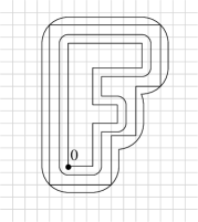
(a) (b)

Figure 5: (a) From inside to outside: an F-shaped set $E$; the enlargement $E_{\rho/4\varphi}$; $E(A)$, the union of the rescaled cubes intersecting $E_{\rho/4\varphi}$; the bounding set $E_{3\rho/4\varphi}$. The grid shows the cubes in the definition of $E(A)$, rescaled to have side length $1/n\varphi$. The parameters $\rho,n$ satisfy $\rho n=2\sqrt{d}$. (b) From inside to outside (scaled by $\varphi$ compared to part (a)): the prospective subset $x+\varphi E$ of $\mathbb{T}^{d}\setminus W_{\rho}[0,t]$; the approximating grid-aligned set $x^{\prime}+\varphi E(A)$; the taboo set $x+(\varphi E)_{\rho}$ that the Brownian motion must not visit.

Given $x\in\mathbb{T}^{d}$, let $x^{\prime}\in G_{n}$ satisfy $d(x,x^{\prime})\leq\sqrt{d}/2n$. Then $x+\varphi E\subset x^{\prime}+(\varphi E)_{\sqrt{d}/2n}\subset x^{\prime}+\varphi E(A)\subset x+(\varphi E(A))_{\sqrt{d}/2n}\subset x+(\varphi E)_{\rho}$ since $\sqrt{d}/2n\leq\rho/4$ and $\varphi E(A)\subset(\varphi E)_{3\rho/4}$. See Fig. 5(b). This proves (4.2); (4.3) follows immediately because $(x+\varphi E)\cap W_{\rho}[0,t]=\varnothing$ is equivalent to $(x+(\varphi E)_{\rho})\cap W[0,t]=\varnothing$.

Similarly, since $(\varphi E)_{\rho/4}\subset\varphi E(A)$ and since $(x+\varphi E)\cap W_{\tilde{\rho}}[0,t]\neq\varnothing$ is equivalent to $(x+(\varphi E)_{\tilde{\rho}})\cap W[0,t]\neq\varnothing$, the inclusion in (4.4) follows. ∎

4.1.1 Proof of Theorem 1.3

In this section we prove the following theorem, of which Theorem 1.3 is the special case with $S(t)=\mathbb{T}^{d}$.

Theorem 4.1

Fix non-negative functions $t\mapsto\rho(t)$ and $t\mapsto h(t)$ satisfying

$$\lim_{t\to\infty}\frac{\rho(t)}{\varphi_{d}(t)}=0,\qquad\lim_{t\to\infty}\frac{\log[h(t)/\varphi_{d}(t)]}{\log t}\leq 0,$$ (4.5)

and collections of points $(S(t))_{t>1}$ in $\mathbb{T}^{d}$ such that $\max_{x\in\mathbb{T}^{d}}d(x,S(t))\leq h(t)$ for all $t>1$. Then, for any $E\subset\mathbb{R}^{d}$ compact with $\operatorname{Cap}E<\kappa_{d}$,

$$\log\mathbb{P}\left((x+\varphi_{d}(t)E)\cap W_{\rho(t)}[0,t]\neq\varnothing\;\forall x\in S(t)\right)\leq-t^{J_{d}(\operatorname{Cap}E)+o(1)},\qquad t\to\infty.$$ (4.6)

Proof

Fix $E\subset\mathbb{R}^{d}$ compact with $\operatorname{Cap}E<\kappa_{d}$, and let $\delta>0$ be arbitrary with $\operatorname{Cap}E+\delta<\kappa_{d}$. By Proposition 5(a), we can choose $r>0$ so that $\operatorname{Cap}(E_{r})\leq\operatorname{Cap}E+\tfrac{1}{2}\delta$. If $E_{r}$ is not already connected, then enlarge it to a connected set $E^{\prime}\supset E_{r}$ by adjoining a finite number of line segments (this is possible because $E_{r}$ is the $r$-enlargement of a compact set). Doing so does not change the capacity, so we may apply Proposition 5(a) again to find $r^{\prime}>0$ so that $\operatorname{Cap}((E^{\prime})_{r^{\prime}})\leq\operatorname{Cap}E+\delta$.

Define $\rho_{0}(t)=r^{\prime}\varphi_{d}(t)$ and $n(t)=\left\lceil 2\big{.}\smash{\sqrt{d}}/\rho_{0}(t)\right\rceil$, so that $\rho_{0}(t)n(t)\geq 2\sqrt{d}$ and the condition (3.17) from Proposition 8 holds. Since $\rho(t)/\varphi_{d}(t)\to 0$, we may choose $t$ sufficiently large so that $\rho(t)\leq\tfrac{1}{4}\rho_{0}(t)$.

Apply Lemma 7 to $E^{\prime}$ with $\rho=\rho_{0}(t)$, $\tilde{\rho}=\rho(t)$, and $\varphi=\varphi_{d}(t)$. Note that if $(x+\varphi_{d}(t)E)\cap W_{\rho(t)}[0,t]\neq\varnothing$ for all $x\in S(t)$, then $(x+\varphi_{d}(t)E(A))\cap W[0,t]\neq\varnothing$ for all $x\in S(t)$, where $\operatorname{Cap}E(A)\leq\operatorname{Cap}((E^{\prime})_{\rho/\varphi})=\operatorname{Cap}((E^{\prime})_{r^{\prime}})\leq\operatorname{Cap}E+\delta$. By Proposition 8 with $\kappa=\operatorname{Cap}E+\delta$, this event has a probability that is at most $\exp[-t^{J_{d}(\operatorname{Cap}E)-O(\delta)}]$, and taking $\delta\downarrow 0$ we get the desired result. ∎

4.1.2 Proof of Theorem 1.1

Proof

First consider $\kappa<\kappa_{d}$. Since $I_{d}(\kappa)$ is infinite for such $\kappa$, it suffices to show that $\lim_{t\to\infty}\log\mathbb{P}(\kappa^{*}(t,\rho(t))\leq\kappa\varphi^{d-2})/\log t=-\infty$. Let $\kappa<\kappa^{\prime}<\kappa_{d}$, and take $E$ to be a ball of capacity $\kappa^{\prime}$. If $\kappa^{*}(t,\rho(t))\leq\kappa\varphi^{d-2}$, then no translate $x+\varphi_{d}(t)E$, $x\in\mathbb{T}^{d}$, can be a subset of $\mathbb{T}^{d}\setminus W_{\rho(t)}[0,t]$. Applying Theorem 1.3, we conclude that $\mathbb{P}(\kappa^{*}(t,\rho(t))\leq\kappa\varphi^{d-2})\leq\exp[-t^{J_{d}(\kappa)+o(1)}]$, which implies the desired result.

Next consider the LDP upper bound for $\kappa\geq\kappa_{d}$. Since $\kappa\mapsto I(\kappa)$ is increasing and continuous on $[\kappa_{d},\infty]$, it suffices to show that $\mathbb{P}(\kappa^{*}(t,\rho(t))\geq\kappa\varphi^{d-2})\leq t^{-I_{d}(\kappa)+o(1)}$ for $\kappa>\kappa_{d}$. Therefore, suppose that $x+\varphi_{d}(t)E\subset\mathbb{T}^{d}\setminus W_{\rho(t)}[0,t]$ for some $x\in\mathbb{T}^{d}$ and $E\subset\mathbb{R}^{d}$ compact with $\operatorname{Cap}E\geq\kappa$. As in the proof of Theorem 4.1, define $n(t)=\left\lceil 2\big{.}\smash{\sqrt{d}}/\rho(t)\right\rceil$. Lemma 7 gives $(x^{\prime}+\varphi_{d}(t)E(A))\cap W[0,t]=\varnothing$ for some $x^{\prime}\in G_{n(t)}$ and $\operatorname{Cap}E(A)\geq\operatorname{Cap}E\geq\kappa$. The condition in (1.17) on $\rho(t)$ implies the condition in (3.3) on $n(t)$, and therefore we may apply Proposition 6 to conclude that $\mathbb{P}(\kappa^{*}(t,\rho(t))\geq\kappa\varphi^{d-2})\leq t^{-I_{d}(\kappa)+o(1)}$.

Finally, the LDP lower bound for $\kappa\geq\kappa_{d}$ will follow (with $E$ the ball of capacity $\kappa$, say) from the lower bound proved for Theorem 1.4 (see Section 4.2). ∎

4.1.3 Proof of Theorem 1.2

Proof

As in the proof of Theorem 1.1, the lower bound will follow from the more specific lower bound proved for Theorem 1.4 (see Section 4.2).

Choose $n(t)$ such that $n(t)\geq 2\sqrt{d}/\rho(t)$ and the hypotheses of Proposition 7 hold. (The conditions on $n(t)$ are mutually consistent because $2\sqrt{d}/\rho(t)=O(1/\varphi_{d}(t))$.) Given any component $C$ containing a ball of radius $\rho(t)$ and having the form $C=x+\varphi_{d}(t)E$ for $\operatorname{Cap}E\geq\kappa$, apply Lemma 7 to find $x^{\prime}_{C}\in G_{n(t)}$ and $A_{C}\in\mathcal{A}^{\boxempty}$ such that $C\subset x^{\prime}_{C}+\varphi_{d}(t)E(A_{C})\subset C_{\rho(t)}\subset\mathbb{T}^{d}\setminus W[0,t]$. The pairs $(x^{\prime}_{C},E(A_{C}))$ so constructed must be distinct: for $C^{\prime}\neq C$, we have $x^{\prime}_{C^{\prime}}+\varphi_{d}(t)E(A_{C^{\prime}})\subset C^{\prime}_{\rho(t)}\subset(\mathbb{T}^{d}\setminus C)_{\rho(t)}=\mathbb{T}^{d}\setminus C_{-\rho(t)}$, and since $C_{-\rho(t)}$ is non-empty by assumption, it follows that $C\nsubseteq x^{\prime}_{C^{\prime}}+\varphi_{d}(t)E(A_{C^{\prime}})$. We therefore conclude that $\chi_{\rho(t)}(t,\kappa)\leq\chi_{+}^{\boxempty}(t,n(t),\kappa)$, so the required upper bound follows from Proposition 7. ∎

4.1.4 Proof of Proposition 1

Proof

Abbreviate $\varphi=\varphi_{d}(t),\rho=\rho(t)$. It suffices to bound the probability that $\mathbb{T}^{d}\setminus W_{\rho}[0,t]$ has a component of diameter at least $\tfrac{1}{2}$, since the mapping $x+y\mapsto y$ from $B(x,r)\subset\mathbb{T}^{d}$ to $B(0,r)\subset\mathbb{R}^{d}$ is a well-defined local isometry if $r<\tfrac{1}{2}$.

Suppose that $x\in\mathbb{T}^{d}\setminus W_{\rho}[0,t]$ belongs to a connected component intersecting $\partial B(x,\tfrac{1}{2})$. Then there is a bounded connected set $E\subset\mathbb{R}^{d}$ such that $(x+\varphi E)\cap W_{\rho}[0,t]$ and $E\cap\partial B(0,\tfrac{1}{2}\varphi^{-1})\neq\varnothing$ (see Fig. 6). Define $n=n(t)=\left\lceil 2\big{.}\smash{\sqrt{d}/\rho}\right\rceil$ and apply Lemma 7 to conclude that $(x^{\prime}+\varphi E(A))\cap W[0,t]=\varnothing$ with $E\subset E(A)$, $A\in\mathcal{A}^{\boxempty}$, $x^{\prime}\in G_{n}$. Since $E(A)$ contains $E$, it has diameter at least $\tfrac{1}{2}\varphi^{-1}$, so $A$ has diameter at least $\tfrac{1}{2}n$ and must consist of at least $n/(2\sqrt{d})$ unit cubes. Since $\rho=o(\varphi)$ and $\varphi=t^{-d/(d-2)+o(1)}$, we have $n\geq t^{d/(d-2)+o(1)}$. The hypothesis in (1.17) implies that $n\varphi=o((\log t)^{1/d})$, as in condition (3.3) from Proposition 6. Therefore $\operatorname{Vol}E(A)\geq(n\varphi)^{-d}n/(2\sqrt{d})\geq t^{d/(d-2)+o(1)}$, and in particular $\operatorname{Vol}E(A)\to\infty$. By (1.45), $\operatorname{Cap}E(A)\to\infty$ also. Thus, if $\mathbb{T}^{d}\setminus W_{\rho}[0,t]$ has a component of diameter at least $\tfrac{1}{2}$, then the event in Proposition 6 occurs, with $\kappa$ arbitrarily large for $t\to\infty$. By Proposition 6, the probability of this occuring is negligible, as claimed. ∎

Figure 6: A large connected component of $\mathbb{T}^{d}\setminus W_{\rho}[0,t]$ that is not isometric to a subset of $\mathbb{R}^{d}$ (shading) and a possible choice of the set $x+\varphi E$ (dark shading).

This proof is unchanged if the radius $\tfrac{1}{2}$ is replaced by any $\delta\in(0,\tfrac{1}{2})$, which shows that the maximal diameter $D(t,\rho(t))$ satisfies $D(t,\rho(t))\to 0$ in $\mathbb{P}$-probability when (1.17) holds (see Section 1.6.5).

4.2 Proof of Theorem 1.4

In Theorems 1.1–1.3 we deal with components that contain a subset $x+\varphi_{d}(t)E$ of a given form. Theorem 1.4 adds the requirement that the component containing such a subset should not extend further than distance $\delta\varphi_{d}(t)$ from $x+\varphi_{d}(t)E$. In the proof, we will bound the probability that the component extends no further than distance $\rho(t)$ from $x+\varphi_{d}(t)E$, but only for sets $E\in\mathcal{E}^{\boxempty}_{c}$ of the following kind: define

$$\mathcal{E}^{\boxempty}_{c}=\left\{\text{$E\in\mathcal{E}_{c}$: $E=\tfrac{1}{n}A$ for some $A\in\mathcal{A}^{\boxempty}$}\right\}$$ (4.7)

to be the collection of sets in $\mathcal{E}_{c}$ that are rescalings of lattice animals.

Note that, unlike in Section 3, the scaling factor $\tfrac{1}{n}$ in (4.7) is fixed and does not depend on $t$. We begin by showing that the collection $\mathcal{E}^{\boxempty}_{c}$ is dense in $\mathcal{E}_{c}$.

Lemma 8

Given $E\in\mathcal{E}_{c}$ and $\delta>0$, there exists $E^{\boxempty}\in\mathcal{E}^{\boxempty}_{c}$ with $E\subset E^{\boxempty}\subset E_{\delta}$.

Lemma 8 will allow us to prove Theorem 1.4 only for $E\in\mathcal{E}^{\boxempty}_{c}$.

Proof

For $y\notin E$, define

$$b(y)=\sup\left\{r>0\colon\,y\text{ belongs to the unbounded component of }\mathbb{R}^{d}\setminus E_{r}\right\}.$$ (4.8)

Since $\mathbb{R}^{d}\setminus E$ is open and connected, $b(y)$ is continuous and positive on $\mathbb{R}^{d}\setminus E$. By compactness, we may choose $\eta\in(0,\delta)$ such that $b(y)>\eta$ for $y\notin E_{\delta}$. Apply Lemma 7 (with $\rho$ and $\varphi$ replaced by $\eta$ and 1, and $n$ sufficiently large) to find $E^{\prime}=\tfrac{1}{n}A$ with $E\subset E^{\prime}\subset E_{\eta}$. The set $E^{\prime}$ is a rescaled lattice animal, but $\mathbb{R}^{d}\setminus E^{\prime}$ might not be connected. However, if $y$ belongs to a bounded component of $\mathbb{R}^{d}\setminus E^{\prime}$, then $b(y)\leq\eta$ by construction: since $E^{\prime}\subset E_{\eta}$, $y$ cannot belong to the unbounded component of $\mathbb{R}^{d}\setminus E_{\eta}$. By choice of $\eta$, it follows that every bounded component of $\mathbb{R}^{d}\setminus E^{\prime}$ is contained in $E_{\delta}$. Thus, if we define $E^{\boxempty}$ to be $E^{\prime}$ together with these bounded components (see Fig. 7), then $E^{\boxempty}\in\mathcal{E}_{c}^{\boxempty}$ and $E^{\boxempty}\subset E_{\delta}$, as claimed. ∎

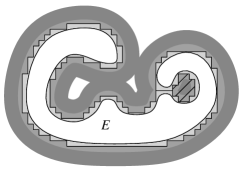
Figure 7: A set $E$ (white) and its enlargement $E_{\delta}$ (dark shading). Every bounded component of $\mathbb{R}^{d}\setminus E_{\delta}$ can reach infinity without touching $E_{\eta}$ (medium shading). A set $E^{\prime}$ (light shading) with $E\subset E^{\prime}\subset E_{\eta}$ may disconnect a region from infinity (diagonal lines), but this region must belong to $E_{\delta}$.

In the proof of Theorem 1.4, we adapt the concept of $(N,\varphi,r,R)$-successful from Definition 1 to formulate the desired event in terms of excursions. To this end we next introduce the sets and events that we will use. In the remainder of this section, we abbreviate $\varphi=\varphi_{d}(t)$, $\rho=\rho(t)$, $I_{d}(\kappa)=I(\kappa)$ and $J_{d}(\kappa)=J(\kappa)$.

Fix $E\in\mathcal{E}_{c}^{\boxempty}$ and $\delta>0$. We may assume that $E\subset B(0,a)$ with $a>\delta$. Let $\eta\in(0,\tfrac{1}{2})$ be small enough that $\kappa_{d}\eta^{d-2}<\operatorname{Cap}E$. Set $r=\varphi^{1-\eta}$, $R=\varphi^{1-2\eta}$, and let $\left\{x_{0},\dotsc,x_{K}\right\}\subset\mathbb{T}^{d}$ denote a maximal collection of points in $\mathbb{T}^{d}$ satisfying $d(x_{0},x_{j})>R$ and $d(x_{j},x_{k})>2R$ for $j\neq k$, so that

$$K=R^{-d-o(1)}=t^{d/(d-2)+O(\eta)}$$ (4.9)

Take $t$ large enough that $\rho<\tfrac{1}{2}\delta\varphi$ and $R<\tfrac{1}{2}$. Set $N=(1+\eta)N_{d}(t,r,R)$ (see (2.5)).

Choose $q=q(t)$ with $q>2a+\delta$, $q\geq\log t$, and $q=(\log t)^{O(1)}$. Let $\left\{y_{1},\dotsc,y_{L}\right\}\subset B(0,2q)\setminus E_{\delta}$ denote a maximal collection of points in $B(0,2q)\setminus E_{\delta}$ satisfying $d(y_{\ell},E)\geq\delta$, $d(y_{\ell},y_{m})\geq\tfrac{1}{2}\rho/\varphi$ for $\ell\neq m$, so that $L=O((q\varphi/\rho)^{d})=(\log t)^{O(1)}$ by (1.17).

(The collection $\left\{y_{1},\dotsc,y_{L}\right\}$ will be used to ensure that a component containing $x_{j}+\varphi E$ is contained in $x_{j}+\varphi E_{\delta}$; see the event $F_{3}(j)$ below. The requirements on $q$ are chosen so that $L$ is suitably bounded, while also allowing us to apply Lemma 5 to deal with components that are relatively far from $x_{j}$.)

Let $Z=\partial(E_{\rho/\varphi})\cup(\cup_{z\in B(0,2a)\cap\eta\mathbb{Z}^{d}}\partial B(z,\eta)\setminus E_{\rho/\varphi})$ (see Fig. 8: $Z$ consists of a $(d-1)$-dimensional shell around $E$ together with a finite number of $(d-1)$-dimensional spheres). Let $\left\{z_{1},\dotsc,z_{M}\right\}\subset Z$ denote a maximal collection of points in $Z$ with $d(z_{m},z_{p})\geq\tfrac{1}{2}\rho/\varphi$ for $m\neq p$. Since $Z$ is $(d-1)$-dimensional, we have $M=O((\rho/\varphi)^{d-1})$.

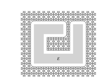
Figure 8: The set $E$ (shaded) and part of the $(d-1)$-dimensional set $Z$.

For $j=1,\dotsc,K$, define the following events.

• $F_{1}(j)=\left\{\frac{1}{2}N\leq N(x_{j},t,r,R)\leq N\right\}$ is the event that $W$ makes between $\tfrac{1}{2}N$ and $N$ excursions from $\partial B(x_{j},r)$ to $\partial B(x_{j},R)$ by time $t$.

• $F_{2}(j)$ is the event that $(x_{j},E_{\rho/\varphi})$ is $(\left\lfloor N\right\rfloor,\varphi,r,R)$-successful.

• $F_{3}(j)$ is the event that, for each $\ell=1,\dotsc,L$, the $i^{\rm th}$ excursion from $\partial B(x_{j},r)$ to $\partial B(x_{j},R)$ hits $x_{j}+B(\varphi y_{\ell},\tfrac{1}{2}\rho)$ for some $i=i(\ell)\in\left\{1,\dotsc,\left\lfloor N/4\right\rfloor\right\}$.

• $F_{4}(j)$ is the event that, for each $m=1,\dotsc,M$, the $i^{\rm th}$ excursion from $\partial B(x_{j},r)$ to $\partial B(x_{j},R)$ hits $x_{j}+B(\varphi z_{m},\tfrac{1}{2}\rho)$ for some $i=i(m)\in\left\{\left\lfloor N/4\right\rfloor+1,\dotsc,\left\lfloor N/2\right\rfloor\right\}$.

• $F_{5}(j)$ is the event that $\mathbb{T}^{d}\setminus W_{\rho}[0,t]$ contains no component of capacity at least $\varphi^{d-2}\operatorname{Cap}E$ disjoint from $B(x_{j},2q\varphi)$.

• $F(j)=F_{1}(j)\cap F_{2}(j)\cap F_{3}(j)$.

• $F_{\rm max}(j)=F_{1}(j)\cap F_{2}(j)\cap F_{3}(j)\cap F_{4}(j)\cap F_{5}(j)$.

Lemma 9

On $F(j)$, the component of $\mathbb{T}^{d}\setminus W_{\rho}[0,t]$ containing $x_{j}+\varphi E$ satisfies condition ($\mathcal{C}(t,\rho,E,E^{\prime})$) with $E^{\prime}=E_{\delta}$. Furthermore, $F_{\rm max}(j)\subset F_{\rho}(t,E,E_{\delta})$ for $t$ sufficiently large.

Proof

Note that if $F_{1}(j)\cap F_{2}(j)$ occurs, then $x_{j}+\varphi E\subset\mathbb{T}^{d}\setminus W_{\rho}[0,t]$. If $F_{1}(j)\cap F_{3}(j)$ occurs, then the set $x_{j}+\cup_{\ell=1}^{L}B(\varphi y_{\ell},\tfrac{1}{2}\rho)$ is entirely covered by the Wiener sausage. By choice of $\left\{y_{1},\dotsc,y_{L}\right\}$, this set contains $x_{j}+\left(B(0,2q\varphi)\setminus\varphi E_{\delta}\right)$, and consequently $\left(\mathbb{T}^{d}\setminus W_{\rho}[0,t]\right)\cap B(x_{j},2q\varphi)\subset x_{j}+\varphi E_{\delta}$.

We have therefore shown that, on $F(j)$, $\mathbb{T}^{d}\setminus W_{\rho}[0,t]$ has a component containing $x_{j}+\varphi E$ and satisfying condition $\mathcal{C}(t,\rho,E,E_{\delta})$. To show further that $F_{\rm max}(j)\subset F_{\rho}(t,E,E_{\delta})$, we will show any other component must have capacity smaller than $\varphi^{d-2}\operatorname{Cap}E$.

If $F_{1}(j)\cap F_{4}(j)$ occurs, then $x_{j}+\varphi Z$ is entirely covered by the Wiener sausage, by choice of $\left\{z_{1},\dotsc,z_{M}\right\}$. By choice of $Z$, all components of $B(x_{j},a\varphi)\setminus(x_{j}+\varphi Z)$, other than any components that are subsets of $x_{j}+\varphi E_{\rho/\varphi}=x_{j}+(\varphi E)_{\rho}$, must be contained in a ball of radius $\eta\varphi$, and in particular have capacity at most $\kappa_{d}(\eta\varphi)^{d-2}<\varphi^{d-2}\operatorname{Cap}E$.

Finally, if $F_{5}(j)$ occurs, then the component of largest capacity cannot occur outside $B(x_{j},2q\varphi)$, and therefore must be the component of largest capacity contained in $x_{j}+(\varphi E)_{\rho}$.

It therefore remains to show that the component of largest capacity in $x_{j}+(\varphi E)_{\rho}$ is in fact the component containing $x_{j}+\varphi E$. Suppose that $a\in x_{j}+\varphi E$ is the centre of a $(d-1)$-dimensional ball of radius $\rho$ that is completely contained in some face of $x_{j}+\varphi E$, and let $b$ be a point at distance at most $\rho$ from $a$ along the line perpendicular to the face (see Fig. 9). If both $x_{j}+\varphi E$ and $b$ are contained in $\mathbb{T}^{d}\setminus W_{\rho}[0,t]$, then so is the line segment from $a$ to $b$, so that $b$ belongs to the same component as $x_{j}+\varphi E$.

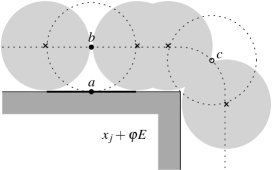
Figure 9: A point $b$ near the centre $a$ of a ball (thicker line) on a face of $x_{j}+\varphi E$, and a point $c$ near the boundary of a face. The Brownian path must not touch the dotted lines, but the Wiener sausage can fill the shaded circles by visiting the crossed points. The point $c$ can belong to a different component than $x_{j}+\varphi E$, but $b$ cannot.

We therefore conclude that, on $F_{\rm max}(j)$, any point of $x_{j}+(\varphi E)_{\rho}$ that is not in the same component as $x_{j}+\varphi E$ must lie within distance $2\rho$ of the boundary of some face of $x_{j}+\varphi E$. Write $H$ for the set of boundaries of faces of $E$. Since $H$ is $(d-2)$-dimensional, its capacity is $0$, and therefore $\operatorname{Cap}((\varphi H)_{2\rho})=\varphi^{d-2}\operatorname{Cap}(H_{2\rho/\varphi})=o(\varphi^{d-2})$ by Proposition 5(a), since $\rho/\varphi\to 0$. In particular, for $t$ sufficiently large the component of largest capacity in $x_{j}+(\varphi E)_{\rho}$ must be the component containing $x_{j}+\varphi E$, which completes the proof of Lemma 9. ∎

Proof (Proof of Theorem 1.4)

Because of the upper bound proved for Theorems 1.1–1.2, we need only prove the lower bounds

$$\mathbb{P}\left(F_{\rho}(t,E,E_{\delta})\right)\geq t^{-I(\operatorname{Cap}E)-o(1)},\qquad\operatorname{Cap}E\geq\kappa_{d},\delta>0.$$ (4.10)

and

$$\chi_{\rho}(t,E,E_{\delta})\geq t^{J(\operatorname{Cap}E)-o(1)}\text{ with high probability,}\qquad\operatorname{Cap}E<\kappa_{d},\delta>0.$$ (4.11)

Moreover, it suffices to prove (4.10)–(4.11) under the assumption that $E\in\mathcal{E}_{c}^{\boxempty}$ and, in (4.10), that $\operatorname{Cap}E>\kappa_{d}$. Indeed, given any $\delta^{\prime}\in(0,\tfrac{1}{2}\delta)$, apply Lemma 8 to find $E^{\boxempty}\in\mathcal{E}_{c}^{\boxempty}$ with $E\subset E^{\boxempty}\subset E_{\delta^{\prime}}$. By adjoining, if necessary, a sufficiently small cube to $E^{\boxempty}$, we may assume that $\operatorname{Cap}E^{\boxempty}>\operatorname{Cap}E$. Apply (4.10)–(4.11) with $E$ and $\delta$ replaced by $E^{\boxempty}$ and $\delta^{\prime}$, respectively. Proposition 5(a) implies that $\operatorname{Cap}E^{\boxempty}\downarrow\operatorname{Cap}E$ as $\delta^{\prime}\downarrow 0$. Since $\kappa\mapsto J(\kappa)$ is continuous, we conclude that the bounds for $E\in\mathcal{E}_{c}$ follows from those for $E\in\mathcal{E}^{\boxempty}_{c}$.

We next relate the left-hand side of (4.10) to the events $F_{1}(j),\dotsc,F_{5}(j)$. Noting that $F_{1}(j)\cap F_{2}(j)\cap F_{1}(k)\cap F_{2}(k)\subset F_{5}(j)^{c}$ for $j\neq k$, Lemma 9 implies that

$$\mathbb{P}\left(F_{\rho}(t,E,E_{\delta})\right) \geq\sum_{j=1}^{K}\mathbb{P}_{x_{0}}(F(j))$$

$$\geq\sum_{j=1}^{K}\mathbb{P}_{x_{0}}(F_{2}(j)\cap F_{3}(j)\cap F_{4}(j))-\sum_{j=1}^{K}\mathbb{P}_{x_{0}}(F_{1}(j)^{c})-\sum_{j=1}^{K}\mathbb{P}_{x_{0}}(F_{1}(j)\cap F_{2}(j)\cap F_{5}(j)^{c}).$$ (4.12)

We will bound each of the sums in the right-hand side of (4.12).

Applying Proposition 3 and (4.9) (and noting that $N_{d}(t,r,R)=t^{\eta+o(1)}$ and that $\tfrac{1}{2}N/N_{d}(t,r,R)=\tfrac{1}{2}(1+\eta)<\tfrac{3}{4}$), we see that the second sum in the right-hand side of (4.12) is at most $t^{d/(d-2)+O(\eta)}\exp[-ct^{\eta+o(1)}]$. This term will be negligible compared to the scale of (4.10).

For the last sum in (4.12), we assume that $\operatorname{Cap}E>\kappa_{d}$ and use Lemma 5. Set $h(t)=2q\varphi$, and note that $h(t)/(\varphi\log t)\geq 1$ by assumption on $q$. If $F_{1}(j)\cap F_{2}(j)\cap F_{5}(j)^{c}$ occurs, then, by Lemma 7, there are lattice animals $A,A^{\prime}\in\mathcal{A}^{\boxempty}$ with $\operatorname{Cap}E(A),\operatorname{Cap}E(A^{\prime})\geq\operatorname{Cap}E$ and a point $x^{\prime}\in\mathbb{T}^{d}\setminus B(x_{j},2q\varphi)$ with $(x_{j}+\varphi E(A))\cap W[0,t]=(x^{\prime}+\varphi E(A^{\prime}))\cap W[0,t]=\varnothing$. By Lemma 5 with $\kappa^{(1)}=\kappa^{(2)}=\operatorname{Cap}E$, we have

$$\mathbb{P}_{x_{0}}(F_{1}(j)\cap F_{2}(j)\cap F_{5}(j)^{c})\leq t^{-d\operatorname{Cap}(E)/[(d-2)\kappa_{d}]-I(\operatorname{Cap}E)+o(1)}.$$ (4.13)

Hence the last sum in (4.12) is at most $t^{-2I(\operatorname{Cap}E)+O(\eta)}$. Since $I(\operatorname{Cap}E)>0$, this term is also negligible, for $\eta$ sufficiently small, compared to the scale of (4.10). (This is the only part of the proof where $\operatorname{Cap}E>\kappa_{d}$ is used.)

We have therefore proved that (4.10) will follow if we can give a suitable lower bound for the first sum on the right-hand side of (4.12). Using again the asymptotics (4.9) for $K$, (4.10) will follow from

$$\mathbb{P}_{x_{0}}\left(F_{2}(j)\cap F_{3}(j)\cap F_{4}(j)\left|\,((\xi^{\prime}_{i}(x_{j}),\xi_{i}(x_{j}))_{i=1}^{N})_{j=1}^{K}\right.\right)\geq t^{-d\operatorname{Cap}E/[(d-2)\kappa_{d}]-O(\eta)}.$$ (4.14)

In fact, (4.14) also implies (4.11). On the event $\cap_{j=1}^{K}F_{1}(j)$ (which occurs with high probability, by Proposition 3), Lemma 9 implies that $\chi_{\rho}(t,E,E_{\delta})$ is at least as large as the number of $j\in\left\{1,\dotsc,K\right\}$ for which $F_{2}(j)\cap F_{3}(j)$ occurs. Since the events $F_{2}(j)\cap F_{3}(j)$ are conditionally independent for different $j$ given the starting and ending points $((\xi^{\prime}_{i}(x_{j}),\xi_{i}(x_{j}))_{i=1}^{N})_{j=1}^{K}$, (4.14) and (4.9) immediately imply that $\chi_{\rho}(t,E,E_{\delta})\geq t^{J_{d}(\kappa)-O(\eta)}$ with high probability (cf. the proof of Proposition 7 in Section 3.2.1).

It therefore remains to prove (4.14). To do so, we will condition on not hitting $x_{j}+(\varphi E)_{\rho}$ and use the following lemma to estimate the conditional probability of hitting small nearby balls. Note that, conditional on the occurence of $F_{2}(j)$ and the starting and ending points $(\xi^{\prime}_{i}(x_{j}),\xi_{i}(x_{j}))_{i=1}^{N}$, the events $F_{3}(j)$ and $F_{4}(j)$ are independent.

Lemma 10

Fix $E\in\mathcal{E}_{c}^{\boxempty}$ and $\delta>0$, and let $0<\rho<\varphi<r<R<\tfrac{1}{2}$. Then there is an $\epsilon>0$ such that if $\rho/\varphi<\epsilon$, $\varphi/r<\epsilon$ and $r/R\leq\tfrac{1}{2}$, then, uniformly in $x\in\mathbb{T}^{d}$, $\xi^{\prime}\in\partial B(x,r)$, and $\xi\in\partial B(x,R)$,

$$\mathbb{P}_{\xi^{\prime},\xi}\!\left(\left.(x+B(\varphi y,\tfrac{1}{2}\rho))\cap W[0,\zeta_{R}]\neq\varnothing\,\right|(x+(\varphi E)_{\rho})\cap W[0,\zeta_{R}]=\varnothing\right)\\ \geq\begin{cases}\epsilon(\varphi/r)^{d-2}(\rho/\varphi)^{d-2},&\text{if }y\in B(0,r/\varphi)\setminus E_{\delta},\\ \epsilon(\varphi/r)^{d-2}(\rho/\varphi)^{\alpha},&\text{if }y\in E_{\delta}\setminus E_{\rho/\varphi},\end{cases}$$ (4.15)

where $\alpha>d-2$ is some constant depending only on $d$.

We give the proof of Lemma 10 in Section A.2.

The event $F_{3}(j)$ says that all $(x_{j},B(y_{\ell},\tfrac{1}{2}\rho/\varphi))$, $\ell=1,\dotsc,L$, are not $(\left\lfloor N/4\right\rfloor,\varphi,r,R)$-successful. Lemma 10 implies (as in the proof of Proposition 4) that, uniformly in $\ell$,

$$\mathbb{P}_{x_{0}}\!\left(\left.(x_{j},B(y_{\ell},\tfrac{1}{2}\rho/\varphi))\text{ is $(\left\lfloor N/4\right\rfloor,\varphi,r,R)$-successful}\,\right|F_{2}(j)\right)$$

$$\quad\leq\left(1-\epsilon(\rho/r)^{d-2}(\rho/\varphi)\right)^{\left\lfloor N/4\right\rfloor}=\exp\left[-\epsilon\left\lfloor N/4\right\rfloor(\varphi/r)^{d-2}(\rho/\varphi)^{d-1}(1+o(1))\right]\!.$$ (4.16)

Recalling (1.3) and (2.5), we have $N(\varphi/r)^{d-2}\geq(d/(d-2)+O(\eta))\log t$, so that

$$\mathbb{P}_{x_{0}}\!\left(\left.\text{some $(x_{j},B(y_{\ell},\tfrac{1}{2}\rho/\varphi))$ is $(\left\lfloor N/4\right\rfloor,\varphi,r,R)$-successful}\,\right|F_{2}(j)\right)$$

$$\quad\leq L\exp\left[-\epsilon\left(\tfrac{1}{4}d/(d-2)+O(\eta)\right)\left(\frac{(\log t)^{1/d}\rho}{\varphi}\right)^{d-2}(\log t)^{2/d}\right]\!.$$ (4.17)

By (1.17), $(\log t)^{1/d}\rho/\varphi\to\infty$, whereas $L=(\log t)^{O(1)}$. Hence, the conditional probability in (4.17) is $o(1)$ and $\mathbb{P}\left(\left.F_{3}(j)\,\right|F_{2}(j)\right)=1-o(1)$.

For $F_{4}(j)$, write $k=\left\lfloor N/2\right\rfloor-\left\lfloor N/4\right\rfloor$ and $p=\epsilon(\varphi/r)^{d-2}(\rho/\varphi)^{\alpha}$. Lemma 10 states that, conditional on $F_{2}(j)$, each ball $x_{j}+B(\varphi z_{m},\tfrac{1}{2}\rho)$ has a probability at least $p$ of being hit during each of the $k$ excursions from $\partial B(x_{j},r)$ to $\partial B(x_{j},R)$ in the definition of $F_{4}(j)$. It follows that $\mathbb{P}\left(\left.F_{4}(j)\,\right|F_{2}(j)\right)$ is at least the probability that a Binomial$(k,p)$ random variable has value $M$ or larger. We have $p\to 0$ and $k-M\to\infty$ as $t\to\infty$, so using Stirling’s approximation, we get

$$\mathbb{P}_{x_{0}}\!\left(\left.F_{4}(j)\,\right|F_{2}(j)\right)\geq\binom{k}{M}p^{M}(1-p)^{k-M}=\frac{k^{k}p^{M}(1-p)^{k-M}}{M^{M}(k-M)^{k-M}(\sqrt{2\pi}+o(1))}\\ \geq\left(\frac{kp}{M}\right)^{M}\frac{(1-p)^{k}}{\sqrt{2\pi}+o(1)}=\exp\left[-M\log(M/kp)-O(kp)-O(1)\right]\!.$$ (4.18)

Observe that $kp=e^{O(1)}N_{d}(t,r,R)(\varphi/r)^{d-2}(\rho/\varphi)^{\alpha}=e^{O(1)}(\rho/\varphi)^{\alpha}\log t$. The assumption $\rho/\varphi\to 0$ implies that $kp=o(\log t)$. On the other hand, recall that $M=O((\varphi/\rho)^{d-1})$, so that $M/kp=e^{O(1)}(\varphi/\rho)^{\alpha+d-1}/\log t$. The hypothesis (1.17) means that $\varphi/\rho=o((\log t))^{1/d}$. Consequently, $M=o((\log t)^{(d-1)/d})$ and $\log(M/kp)\leq O(\log\log t)$. In particular, $M\log(M/kp)\leq o(\log t)$, and we conclude that

$$\mathbb{P}_{x_{0}}\!\left(\left.F_{4}(j)\,\right|F_{2}(j)\right)=\exp\left(-o(\log t)\right)=t^{o(1)}.$$ (4.19)

Combining (4.17), (4.19), and Proposition 4, we obtain

$$\mathbb{P}_{x_{0}}(F_{2}(j)\cap F_{3}(j)\cap F_{4}(j)) =\mathbb{P}_{x_{0}}(F_{2}(j))\mathbb{P}_{x_{0}}\left(\left.F_{3}(j)\,\right|F_{2}(j)\right)\mathbb{P}_{x_{0}}\left(\left.F_{4}(j)\,\right|F_{2}(j)\right)$$

$$=t^{-d\operatorname{Cap}(E_{\rho/\varphi})/[(d-2)\kappa_{d}]+O(\eta)}\,[1-o(1)]\,t^{o(1)}=t^{-d\operatorname{Cap}(E)/[(d-2)\kappa_{d}]+O(\eta)}.$$ (4.20)

We have therefore verified (4.14), and this completes the proof. ∎

4.3 Proof of Proposition 2

Proof

$\mathbb{T}^{d}\setminus W[0,t]$ is open since $W[0,t]$ is the (almost surely) continuous image of a compact set.

Consider first a Brownian motion $\tilde{W}$ in $\mathbb{R}^{d}$. Define

$$\tilde{Z}=\bigcup_{q,q^{\prime}\in\mathbb{Q}}\bigcup_{1\leq i<j\leq d}\left\{(x_{1},\dotsc,x_{d})\in\mathbb{R}^{d}:x_{i}=q,x_{j}=q^{\prime}\right\}$$ (4.21)

and note that $\tilde{Z}$ is the inverse image $\pi_{0}^{-1}(Z)$ of a path-connected, locally path-connected, dense subset $Z=\pi_{0}(\tilde{Z})\subset\mathbb{T}^{d}$ (where $\pi_{0}\colon,\mathbb{R}^{d}\to\mathbb{T}^{d}$ is the canonical projection map). Since $\tilde{Z}$ is the countable union of $(d-2)$-dimensional subspaces, $\tilde{W}\left[0,\infty\right)$ does not intersect $\tilde{Z}$, except perhaps at the starting point, with probability $1$. Projecting onto $\mathbb{T}^{d}$, it follows that $W\left[0,\infty\right)$ intersects $Z$ in at most one point, and in particular $\mathbb{T}^{d}\setminus W\left[0,\infty\right)$ contains a path-connected, locally path-connected, dense subset. This implies the remaining statements in Proposition 2. ∎

5 Proofs of Corollaries 1–5

5.1 Proof of Corollary 1

Proof

(1.24) follows immediately from the more precise statements in (1.25)–(1.26). By monotonicity and continuity, it suffices to show (1.25) for $\operatorname{Cap}E>\kappa_{d}$.

Consider first the lower bounds in (1.25)–(1.26). Replace $E$ by the compact set ${\rm clo}\!\left(E\right)$ (by hypothesis, this does not change the value of $\operatorname{Cap}E$). Let $\kappa>\operatorname{Cap}E$ be arbitrary and use Proposition 5(a) to find $r>0$ such that $\operatorname{Cap}(E_{r})\leq\kappa$. Adjoin finitely many lines to $E_{r}$ to make it into a connected set $E^{\prime}$ (as in the proof of Theorem 4.1) and then adjoin any bounded components of $\mathbb{R}^{d}\setminus E^{\prime}$ to form a set $E^{\prime\prime}\in\mathcal{E}_{c}$ that satisfies the conditions of Theorem 1.4. For $\operatorname{Cap}E\geq\kappa_{d}$, Theorem 1.4 implies that $x+\varphi_{d}(t)E\subset\mathbb{T}^{d}\setminus W[0,t]$ for some $x\in\mathbb{T}^{d}$, with probability at least $t^{J_{d}(\kappa)-o(1)}$. If instead $\operatorname{Cap}E<\kappa_{d}$, then it is no loss of generality to assume that $\kappa<\kappa_{d}$ also. Then Theorem 1.4 shows that there are at least $t^{J_{d}(\kappa)-o(1)}$ components containing translates $x+\varphi_{d}(t)E$; these translates are necessarily disjoint. In both cases we conclude by taking $\kappa\downarrow\operatorname{Cap}E$.

For the upper bounds, we will shrink the set $E$. The results nearly follow from Theorems 1.1–1.2, since the existence of $x+\varphi_{d}(t)E\subset\mathbb{T}^{d}\setminus W[0,t]$ implies the existence of $x+(\varphi_{d}(t)E)_{-\rho(t)}\subset\mathbb{T}^{d}\setminus W_{\rho(t)}[0,t]$. However, the set $E$ might not be connected. To handle this possibility, we will appeal directly to Lemmas 4 and 6.

Let $\kappa\in(\kappa_{d},\operatorname{Cap}E)$ (for (1.25)) or $\kappa\in(0,\operatorname{Cap}E)$ (for (1.26)) be arbitrary. Apply Proposition 5(c) to find an $r>0$ such that $\operatorname{Cap}(E_{-2r})>\kappa$. The enlargement $(E_{-2r})_{r}$ has a finite number $k$ of components, by boundedness. Set $\rho=\rho(t)=r\varphi_{d}(t)$ and choose $n=n(t)$ such that $n(t)\geq 2\sqrt{d}/\rho(t)$ and the hypotheses of Proposition 7 hold. (As in the proof of Theorem 1.2, these conditions on $n(t)$ are mutually consistent.) Apply Lemma 7 to each of the $k$ components of $(E_{-2r})_{r}$ to obtain a set $E^{\boxempty}=\cup_{j=1}^{k}E(A^{(j)})$ satisfying $(E_{-2r})_{r}\subset E^{\boxempty}\subset(E_{-2r})_{2r}\subset E$. Thus, $\operatorname{Cap}E^{\boxempty}\geq\kappa$. Furthermore, given $x\in\mathbb{T}^{d}$ there is $x^{\prime}\in G_{n(t)}$ such that $x^{\prime}+\varphi_{d}(t)E^{\boxempty}\subset x+\varphi_{d}(t)((E_{-2r})_{2r})\subset x+\varphi_{d}(t)E$. Define $h(t)=C\varphi_{d}(t)$, where $C$ is a constant large enough so that $E\subset B(0,C)$. For $\operatorname{Cap}E>\kappa_{d}$, we can then apply Lemma 4 to conclude that $\mathbb{P}(\exists x\in\mathbb{T}^{d}\colon\,x+\varphi_{d}(t)E\subset\mathbb{T}^{d}\setminus W[0,t])\leq t^{J_{d}(\kappa)+o(1)}$. For $\operatorname{Cap}E<\kappa_{d}$, Lemma 6 implies that $\chi(t,E)\leq\chi_{+}^{\boxempty}(t,n(t),\kappa,h(t))\leq t^{J_{d}(\kappa)+o(1)}$ with high probability. In both cases take $\kappa\uparrow\operatorname{Cap}E$. ∎

5.2 Proof of Corollaries 2–3

Proof

Note the scaling relation

$$\lambda(\varphi D)=\varphi^{-2}\lambda(D).$$ (5.1)

Corollaries 2–3 follow from Theorems 1.1, 1.3 and 1.4 because of the inequalities (1.45). Indeed, apart from the fact that the principal Dirichlet eigenvalue $\lambda(E)$ is decreasing in $E$ rather than increasing, the proofs are identical and we will prove only Corollary 3.

Since $\lambda\mapsto I^{\rm Dirichlet}_{d}(\lambda)$ is continuous and decreasing on $\left(0,\lambda_{d}\right]$, it suffices to prove (1.30) and to show that $\mathbb{P}(\varphi_{d}(t)^{2}\lambda(t,\rho(t))\leq\lambda)=t^{-I_{d}^{\rm Dirichlet}(\lambda)+o(1)}$ for $\lambda<\lambda_{d}$.

For (1.30), note that $\mathbb{T}^{d}\setminus W_{\rho(t)}[0,t]$ cannot contain a ball of capacity $>\kappa_{d}(\lambda_{d}/\lambda(t,\rho(t)))^{(d-2)/2}$: by (1.9) and (5.1), the component of $\mathbb{T}^{d}\setminus W_{\rho(t)}[0,t]$ containing such a ball would have an eigenvalue strictly smaller than $\lambda(t,\rho(t))$. In particular, if $\lambda>\lambda_{d}$ and $\lambda(t,\rho(t))\geq\lambda\varphi_{d}(t)^{-2}$, then $\mathbb{T}^{d}\setminus W_{\rho(t)}[0,t]$ cannot contain a ball of capacity $\kappa_{d}\,\varphi_{d}(t)^{d-2}((\lambda_{d}/\lambda)^{(d-2)/2}+\delta)$ for any $\delta>0$. Taking $\delta$ small enough so that $(\lambda_{d}/\lambda)^{(d-2)/2}$ $+\delta<1$, applying Theorem 1.3 with $E$ the ball of capacity $\kappa_{d}((\lambda_{d}/\lambda)^{(d-2)/2}+\delta)$, and letting $\delta\downarrow 0$, we obtain (1.30).

Now take $\lambda<\lambda_{d}$. By Proposition 1, apart from an event of negligible probability, every component $C$ of $\mathbb{T}^{d}\setminus W_{\rho(t)}[0,t]$ can be isometrically identified (under its intrinsic metric) with a bounded open subset $E$ of $\mathbb{R}^{d}$, via $C=x+E$ for some $x\in\mathbb{T}^{d}$. In particular, $\lambda(C)=\lambda(E)$, and we can apply (1.45) to conclude that $\kappa^{*}(t,\rho(t))\geq\operatorname{Cap}E\geq\kappa_{d}(\lambda_{d}/\lambda(C))^{(d-2)/2}$. Applying Theorem 1.1,

$$\mathbb{P}(\varphi_{d}(t)^{2}\lambda(t,\rho(t))\leq\lambda)\leq\mathbb{P}(\kappa^{*}(t,\rho(t))\geq\kappa_{d}(\lambda_{d}/\lambda)^{(d-2)/2}\varphi_{d}(t)^{d-2})\leq t^{-I_{d}^{\rm Dirichlet}(\lambda)+o(1)}.$$ (5.2)

For the reverse inequality, note that Theorem 1.4 implies that $\mathbb{T}^{d}\setminus W_{\rho(t)}[0,t]$ contains a ball of capacity $\kappa_{d}\,\varphi_{d}(t)^{d-2}(\lambda_{d}/\lambda)^{(d-2)/2}$ with probability at least $t^{-I_{d}^{\rm Dirichlet}(\lambda)-o(1)}$. ∎

5.3 Proof of Corollary 4

Proof

Since $r\mapsto I_{d}^{\rm inradius}(r)$ is continuous and strictly increasing on $\left[1,\infty\right)$ and is infinite elsewhere, it suffices to verify (1.35) and show $\mathbb{P}(\rho_{\rm in}(t)>r\varphi_{d}(t))=t^{-I_{d}^{\rm inradius}(r)+o(1)}$ for $r\geq 1$. But the events $\left\{\rho_{\rm in}(t)\leq r\varphi_{d}(t)\right\}$ and $\left\{\rho_{\rm in}(t)>r\varphi_{d}(t)\right\}$ are precisely the event

$$\left\{(x+\varphi_{d}(t)B(0,r))\cap W[0,t]\neq\varnothing\;\forall x\in\mathbb{T}^{d}\right\}$$ (5.3)

and its complement

$$\left\{\exists x\in\mathbb{T}^{d}\colon\,(x+\varphi_{d}(t)B(0,r))\cap W[0,t]=\varnothing\right\}$$ (5.4)

from Theorem 1.3, with $\rho(t)=0$, and equation (1.25) from Corollary 1, with $E=B(0,r)$. ∎

5.4 Proof of Corollary 5

Proof

Recall that $\left\{\rho_{\rm in}(t)>\epsilon\right\}=\left\{\mathcal{C}_{\epsilon}>t\right\}$, so that setting $t=u\psi_{d}(\epsilon)$, $r=\epsilon/\varphi_{d}(u\psi_{d}(\epsilon))$ rewrites the event $\left\{\mathcal{C}_{\epsilon}>u\psi_{d}(\epsilon)\right\}$ as $\left\{\rho_{\rm in}(t)>r\varphi_{d}(t)\right\}$. By (1.38), $r\to(u/d)^{1/(d-2)}$ as $\epsilon\downarrow 0$. It follows that $\mathbb{P}(\mathcal{C}_{\epsilon}>u\psi_{d}(\epsilon))=t^{-I_{d}^{\rm inradius}((u/d)^{1/(d-2)})+o(1)}$ for $u>d$, since $r\mapsto I_{d}^{\rm inradius}(r)$ is continuous on $(1,\infty)$. Noting that $t=\epsilon^{-(d-2)+o(1)}$, this last expression is $\epsilon^{I_{d}^{\rm cover}(u)+o(1)}$. A similar argument proves (1.37). Because $u\mapsto I_{d}^{\rm cover}(u)$ is continuous and strictly increasing on $\left[d,\infty\right)$ and $I_{d}^{\rm cover}(v)=\infty$ otherwise, these two facts complete the proof. ∎

Appendix A Hitting probabilities for excursions

A.1 Unconditioned excursions: proof of Lemma 2

Proof

Since $R<\tfrac{1}{2}$, we may consider $x,\xi^{\prime},\xi,W(t)$ to have values in $\mathbb{R}^{d}$ instead of $\mathbb{T}^{d}$. Furthermore, w.l.o.g. we may assume that $x=0$.

We first remove the effect of conditioning on the exit point $\xi\in\partial B(0,R)$. Define $T=\sup\left\{t<\zeta\colon\,d(0,W(t))\leq r\right\}$ to be the last exit time from $B(0,r)$ before time $\zeta$; note that $E\cap W[0,\zeta_{R}]=E\cap W[0,T]$. Let $\tilde{r}\in(r,R)$ and define $\tilde{\tau}=\inf\left\{t>T\colon\,d(0,W(t))=\tilde{r}\right\}$ to be the first hitting time of $\partial B(0,\tilde{r})$ after time $T$.

Under $\mathbb{P}_{\xi^{\prime}}$ (i.e., without conditioning on the exit point $W(\zeta_{R})$) we can express $(W(t))_{0\leq t\leq\zeta_{R}}$ as the initial segment $(W(t))_{0\leq t\leq\tilde{\tau}}$ followed by a Brownian motion, conditionally independent given $W(\tilde{\tau})$, started at $\tilde{\xi}=W(\tilde{\tau})$ and conditioned to exit $B(0,R)$ before hitting $B(0,r)$. Let $f_{\tilde{r},R}(\tilde{\xi},\cdot)$ denote the density, with respect to the uniform measure $\sigma_{R}$ on $\partial B(0,R)$, of the first hitting point $W(\zeta_{R})$ on $\partial B(0,R)$ for this conditioned Brownian motion. Then for $S\subset\partial B(0,R)$ measurable, we have

$$\mathbb{P}_{\xi^{\prime}}\!\left(E\cap W[0,\zeta_{R}]\neq\varnothing,W(\zeta_{R})\in S\right)=\mathbb{E}_{\xi^{\prime}}\!\left(\mathbbm{1}_{\left\{E\cap W[0,T]\neq\varnothing\right\}}\int_{S}f_{\tilde{r},R}(W(\tilde{\tau}),\xi)d\sigma_{R}(\xi)\right).$$ (A.1)

From (A.1) it follows that the conditioned measure $\mathbb{P}_{\xi^{\prime},\xi}$ satisfies

$$\mathbb{P}_{\xi^{\prime},\xi}(E\cap W[0,\zeta_{R}]\neq\varnothing)=\frac{\mathbb{E}_{\xi^{\prime}}\!\left(\mathbbm{1}_{\left\{E\cap W[0,T]\neq\varnothing\right\}}f_{\tilde{r},R}(W({\tilde{\tau}}),\xi)\right)}{\mathbb{E}_{\xi^{\prime}}\!\left(f_{\tilde{r},R}(W({\tilde{\tau}}),\xi)\right)}.$$ (A.2)

(More precisely, we would conclude (A.2) for $\sigma_{R}$-a.e. $\xi$, but by a continuity argument we can take (A.2) to hold for all $\xi$.)

Now choose $\tilde{r}$ in such a way that $R/\tilde{r}\to\infty,\tilde{r}/r\to\infty$, for instance, $\tilde{r}=\sqrt{rR}$. Since $R/\tilde{r}\to\infty$, we have $f_{\tilde{r},R}(\tilde{\xi},\xi)=1+o(1)$, uniformly in $\tilde{\xi},\xi$. Therefore

$$\mathbb{P}_{\xi^{\prime},\xi}(E\cap W[0,\zeta_{R}]\neq\varnothing) =[1+o(1)]\,\mathbb{P}_{\xi^{\prime}}(E\cap W[0,\zeta_{R}]\neq\varnothing)$$

$$=[1+o(1)]\left(\big{.}\mathbb{P}_{\xi^{\prime}}(E\cap W\left[0,\infty\right)\neq\varnothing)-\mathbb{P}_{\xi^{\prime}}(E\cap W\left[\zeta_{R},\infty\right)\neq\varnothing)\right)\!.$$ (A.3)

By the Markov property, the last term in (A.1) is the probability of hitting $E$ when starting from some point $W(\zeta_{R})\in\partial B(0,R)$ (averaged over the value of $W(\zeta_{R})$). Since $R/r\to\infty$, this will be shown to be an error term, and the proof will have been completed, once we show that

$$\mathbb{P}_{\xi^{\prime}}\!\left(W\left[0,\infty\right)\cap E\neq\varnothing\right)=\frac{\operatorname{Cap}E}{\kappa_{d}\,r^{d-2}}\,[1+o(1)]\qquad\text{as }r/\epsilon\to\infty.$$ (A.4)

Note that (A.4) is essentially the limit in (1.11), taken uniformly over the choice of $E\subset B(0,\epsilon)$.

To show (A.4), let $g_{\epsilon}(\xi^{\prime},\cdot)$ denote the density, with respect to the uniform measure $\sigma_{\epsilon}$ on $\partial B(0,\epsilon)$, of the first hitting point of $\partial B(0,\epsilon)$ for a Brownian motion started at $\xi^{\prime}$ and conditioned to hit $B(0,\epsilon)$. Then

$$\mathbb{P}_{\xi^{\prime}}\!\left(W\left[0,\infty\right)\cap E\neq\varnothing\right)=\frac{\epsilon^{d-2}}{r^{d-2}}\int_{\partial B(0,\epsilon)}\mathbb{P}_{y}\!\left(W\left[0,\infty\right)\cap E\neq\varnothing\right)g_{\epsilon}(\xi^{\prime},y)d\sigma_{\epsilon}(y).$$ (A.5)

Since $r/\epsilon\to\infty$, we have $g_{\epsilon}(\xi^{\prime},y)\to 1$ uniformly in $\xi^{\prime},y$. Hence (A.4) follows from (A.5) and (2.15). ∎

A.2 Excursions avoiding an obstacle: proof of Lemma 10

Proof

It suffices to bound from below

$$\mathbb{P}_{\xi^{\prime},\xi}\!\left(W[0,\zeta_{R}]\text{ intersects $x+B(\varphi y,\tfrac{1}{2}\rho)$ but not }x+(\varphi E)_{\rho}\right),$$ (A.6)

since conditioning on $(x+(\varphi E)_{\rho})\cap W[0,\zeta_{R}]=\varnothing$ can only increase the probability in (A.6). Moreover, as in the proof of Lemma 2, we may replace $\mathbb{P}_{\xi^{\prime},\xi}$ by $\mathbb{P}_{\xi^{\prime}}$, using now that the densities $f_{\tilde{r},R}$ and $g_{\epsilon}$ are bounded away from $0$ and $\infty$ when $r\leq\tfrac{1}{2}R$.

Fix $E\in\mathcal{E}_{c}^{\boxempty}$, so that $E=\tfrac{1}{n}A$ for some $A\in\mathcal{A}^{\boxempty}\cap\mathcal{E}_{c}$ and $n\in\mathbb{N}$, and fix $\delta>0$ (we may assume that $\delta<1/(2n)$). By assumption, $E$ is bounded, say $E\subset B(0,a)$. By adjusting $\epsilon$, we may assume that $\rho/\varphi<a$ (so that $(\varphi E)_{\rho}\subset B(0,2a\varphi)$) and $r>4a\varphi$. We distinguish between three cases:

$\bullet$ $y\in B(0,3a)\setminus E_{\delta}$. Consider $w\in\mathbb{Z}^{d}\setminus A$. Because $A\in\mathcal{E}_{c}$, there is a finite path of open cubes with centres $w_{0},w_{1},\dots,w_{k}\in\mathbb{Z}^{d}$ such that $w_{0}\in\mathbb{Z}^{d}\setminus B(0,3an)$, $w_{k}=w$, $d(w_{j-1},w_{j})=1$ and ${\rm int}\!\left(\cup_{j=0}^{k}(w_{j}+[-\tfrac{1}{2},\tfrac{1}{2}]^{d})\right)\cap A=\varnothing$. By compactness, the length $k$ of such paths may be taken to be uniformly bounded. Hence, if $\rho/\varphi<\delta/2$, then, given $\xi^{\prime\prime}\in\partial B(x,3a\varphi)$, there is a path $\Gamma\subset B(x,3a\varphi)$ from $\xi^{\prime\prime}$ to $x+\varphi y$ consisting of a finite number of line segments, each of length at most $\varphi$, such that $\Gamma_{\delta\varphi/2}\cap(x+(\varphi E)_{\rho})=\Gamma_{\delta\varphi/2}\cap(x+\varphi(E_{\rho/\varphi}))=\varnothing$. Moreover, the number of line segments can be taken to be bounded uniformly in $y$ and $\xi^{\prime\prime}$. In fact, $\Gamma$ can be chosen as the union of line segments between points $x+\varphi w_{0}/n,\dotsc,x+\varphi w_{k}/n$ as above, together with a bounded number of line segments to join $\xi^{\prime\prime}$ to $x+\varphi w_{0}/n$ in $B(x,3a\varphi)\setminus B(x,2a\varphi)$ and to join $x+\varphi w_{k}/n$ to $x+\varphi y$ in the cube $x+(\varphi/n)(w+[-\tfrac{1}{2},\tfrac{1}{2}]^{d})$ containing $y$ (see Fig. 10)

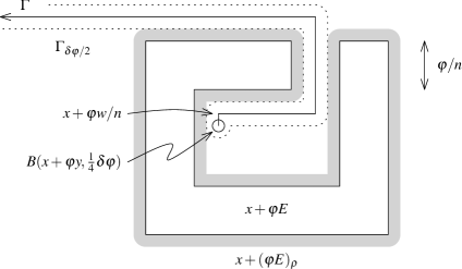
Figure 10: The path $\Gamma$ reaching $x+\varphi y$. The sets $\Gamma_{\delta\varphi/2}$ and $x+(\varphi E)_{\rho}=x+\varphi(E_{\rho/\varphi})$ are depicted for the worst-case scenario where the parameters $\rho/\varphi<\delta/2<1/4n$ are equal.

From $\xi^{\prime}\in\partial B(x,r)$, the Brownian path reaches $\partial B(x,3a\varphi)$ before $\partial B(x,R)$ with probability $(r^{-(d-2)}-R^{-(d-2)})/((3a\varphi)^{-(d-2)}-R^{-(d-2)})$. By our assumptions, this is at least $c_{1}(\varphi/r)^{d-2}$ for some $c_{1}>0$. Uniformly in the first hitting point $\xi^{\prime\prime}$ of $\partial B(x,3a\varphi)$, there is a positive probability of hitting $\partial B(x+\varphi y,\tfrac{1}{4}\delta\varphi)$ via $\Gamma_{\delta\varphi/2}$ before hitting $\partial B(x,4a\varphi)$. The probability of next hitting $\partial B(x+\varphi y,\tfrac{1}{2}\rho)$ before $\partial B(x+\varphi y,\tfrac{1}{2}\delta\varphi)$ is

$$[(\tfrac{1}{4}\delta\varphi)^{-(d-2)}-(\tfrac{1}{2}\delta\varphi)^{-(d-2)}]/[(\tfrac{1}{2}\rho)^{-(d-2)}-(\tfrac{1}{2}\delta\varphi)^{-(d-2)}],$$ (A.7)

which is at least $c_{2}(\rho/\varphi)^{d-2}$ for some $c_{2}>0$. Thereafter there is a positive probability of returning to $\partial B(x,r)$ without hitting $x+(\varphi E)_{\rho}$, via $\Gamma_{\delta\varphi/2}$. Combining these probabilities gives the required bound.

$\bullet$ $y\in E_{\delta}\setminus E_{\rho/\varphi}$. We have $y\in\tfrac{1}{n}(w+[-\tfrac{1}{2},\tfrac{1}{2}]^{d})$ for some $w\in\mathbb{Z}^{d}$. Write $C_{\theta}(y,\tfrac{1}{n}w)$ for the cone with vertex $y$, central angle $\theta$, and axis the ray from $y$ to $\tfrac{1}{n}w$. We can choose the angle $\theta$ and a constant $c_{3}>0$ small enough (in a manner depending only on $d$) so that $C_{\theta}(y,\tfrac{1}{n}w)\cap E_{\rho/\varphi}\cap B(y,(1+c_{3})d(y,w))=\varnothing$. With $\theta$ and $c_{3}$ fixed, we can choose $c_{4}>0$ so that every point of $B(\tfrac{1}{n}w,c_{4})$ is a distance at least $c_{5}>0$ from $\partial C_{\theta}(y,\tfrac{1}{n}w)$ and $\partial B(y,(1+c_{3})d(y,\tfrac{1}{n}w))$ (see Fig. 11).

Figure 11: Cones $C_{\theta}(y,\tfrac{1}{n}w)$ and parts of balls $B(y,\rho/(2\varphi))$ and $B(y,(1+c_{3})d(y,\tfrac{1}{n}w))$ for three choices of $y$. The outer square is the cube $\tfrac{1}{n}(w+[-\tfrac{1}{2},\tfrac{1}{2}]^{d})$ containing $y$. The dashed line shows the greatest possible extent of $E_{\rho/\varphi}$. At least one face of the cube is not contained in $E$, resulting in a conduit to the outside of the cube (dotted lines). The ball $B(\tfrac{1}{n}w,c_{4})$ in the centre is uniformly bounded away from the sides of the cones and from the other balls. On the left the parameters $\rho/\varphi<1/4n$ are depicted as equal. On the right is the more relevant situation $\rho/\varphi\ll 1/(4n)$.

Under these conditions, there is a probability at least $c_{6}(\rho/\varphi)^{\alpha}$ for a Brownian path started from a point of $\partial B(x+\varphi w/n,c_{4}\varphi)$ to reach $\partial B(x+\varphi y,\tfrac{1}{2}\rho)$ before hitting $\partial B(x+\varphi y,\varphi(1+c_{3})d(y,w))\cup\partial(x+\varphi C_{\theta}(y,w))$, and then to reach $\partial B(x+\varphi y,\varphi d(y,w))$ before hitting $\partial(x+\varphi C_{\theta}(y,w))$. The rest of the proof proceeds as in the previous case.

$\bullet$ $y\in B(0,r/\varphi)\setminus B(0,3a)$. Let $b=d(0,y)\in[3a,r/\varphi]$. The probability that a Brownian path started from $\xi^{\prime}$ first hits $\partial B(x,b\varphi)$ without hitting $\partial B(x,R)$, then hits $\partial B(x+\varphi y,\tfrac{1}{12}b\varphi)$ without hitting $\partial B(x,\tfrac{2}{3}b\varphi)$, then hits $\partial B(x+\varphi y,\tfrac{1}{2}\rho)$ before hitting $\partial B(x+\varphi y,\tfrac{1}{6}b\varphi)$, and finally exits $B(x,R)$ without hitting $\partial B(x,\tfrac{2}{3}b\varphi)$, is at least $[c_{7}(b\varphi/r)^{d-2}][c_{8}][c_{9}(\rho/(b\varphi))^{d-2}][c_{10}]$. Since $x+(\varphi E)_{\rho}\subset B(x,2a\varphi)\subset B(x,\tfrac{2}{3}b\varphi)$, this is the required bound. ∎

- (1) Bandle, C.: Isoperimetric Inequalities and Applications. No. 7 in Monographs and Studies in Mathematics. Pitman (1980)
- (2) Benjamini, I., Sznitman, A.S.: Giant component and vacant set for random walk on a discrete torus. J. European Math. Soc. 10(1), 133–172 (2008)
- (3) van den Berg, M.: Heat equation on the arithmetic von Koch snowflake. Probab. Theory Rel. Fields 118, 17–36 (2000)
- (4) van den Berg, M., Bolthausen, E.: Area versus capacity and solidification in the crushed ice model. Probab. Theory Rel. Fields 130, 69–108 (2004)
- (5) van den Berg, M., Bolthausen, E., den Hollander, F.: Moderate deviations for the volume of the Wiener sausage. Ann. Math. 153(2), 355–406 (2001)
- (6) van den Berg, M., Bolthausen, E., den Hollander, F.: Heat content and inradius for regions with a Brownian boundary (2012). arXiv:1304.0579[math.PR]
- (7) van den Berg, M., den Hollander, F.: Asymptotics for the heat content of a planar region with a fractal polygonal boundary. Proc. London Math. Soc. 78(3), 627–661 (1999)
- (8) Burkholder, D.L.: Exit times of Brownian motion, harmonic majorization, and Hardy spaces. Adv. Math. 26(2), 182–205 (1977)
- (9) Dembo, A., Peres, Y., Rosen, J.: Brownian motion on compact manifolds: cover time and late points. Electron. J. Probab. 8(15), 1–14 (2003)
- (10) Dembo, A., Peres, Y., Rosen, J., Zeitouni, O.: Cover times for Brownian motion and random walks in two dimensions. Ann. Math. 160(2), 433–464 (2004)
- (11) Doob, J.L.: Classical Potential Theory and Its Probabilistic Counterpart. No. 262 in Grundlehren der mathematischen Wissenschaften. Springer-Verlag (1984)
- (12) Klarner, D.A.: Cell growth problems. Can. J. Math. 19, 851–863 (1967)
- (13) Levine, L., Peres, Y.: Strong spherical asymptotics for rotor-router aggregation and the divisible sandpile. Potential Anal. 30, 1–27 (2009)
- (14) Matheron, G.: Random Sets and Integral Geometry. Wiley series in probability and mathematical statistics. Wiley (1975)
- (15) Mejía Miranda, Y., Slade, G.: The growth constants of lattice trees and lattice animals in high dimensions. Electron. Comm. Probab. 16(13), 129–136 (2011)
- (16) Molchanov, I.: Theory of Random Sets. Probability and its Applications. Springer (2005)
- (17) Pólya, G., Szegö, G.: Isoperimetric Inequalities in Mathematical Physics. No. 27 in Annals of Mathematics Studies. Princeton University Press (1951)
- (18) Popov, S., Teixeira, A.: Soft local times and decoupling of random interlacements (2012). arXiv:1212.1605 [math.PR]
- (19) Port, S.C., Stone, C.J.: Brownian Motion and Classical Potential Theory. Probability and Mathematical Statistics. Academic Press (1978)
- (20) Sidoravicius, V., Sznitman, A.S.: Percolation for the vacant set of random interlacements. Comm. Pure Appl. Math. 62(6), 831–858 (2009)
- (21) Sznitman, A.: Brownian Motion, Obstacles and Random Media. Springer Monographs in Mathematics. Springer (1998)
- (22) Sznitman, A.S.: Vacant set of random interlacements and percolation. Ann. Math. 171(3), 2039–2087 (2010)
- (23) Sznitman, A.S.: On scaling limits and Brownian interlacements (2012). arXiv:1209.4531 [math.PR]
- (24) Teixeira, A., Windisch, D.: On the fragmentation of a torus by random walk. Comm. Pure Appl. Math. 64(12), 1599–1646 (2011)