An asymptotic preserving scheme based on a new formulation for NLS in the semiclassical limit

Abstract.

We consider the semiclassical limit for the nonlinear Schrödinger equation. We introduce a phase/amplitude representation given by a system similar to the hydrodynamical formulation, whose novelty consists in including some asymptotically vanishing viscosity. We prove that the system is always locally well-posed in a class of Sobolev spaces, and globally well-posed for a fixed positive Planck constant in the one-dimensional case. We propose a second order numerical scheme which is asymptotic preserving. Before singularities appear in the limiting Euler equation, we recover the quadratic physical observables as well as the wave function with mesh size and time step independent of the Planck constant. This approach is also well suited to the linear Schrödinger equation.

1. Introduction and main results

1.1. Motivation

We consider the cubic, defocusing, nonlinear Schrödinger equation (NLS)

$$i\varepsilon{\partial}_{t}u^{\varepsilon}+\frac{\varepsilon^{2}}{2}\Delta u^{\varepsilon}=|u^{\varepsilon}|^{2}u^{\varepsilon},\quad(t,x)\in{\mathbb{R}}_{+}\times{\mathbb{R}}^{d},$$ (1.1)

with WKB type initial data

$$u^{\varepsilon}(0,x)=a_{0}(x)e^{i\phi_{0}(x)/\varepsilon},$$ (1.2)

the functions $a_{0}$ and $\phi_{0}$ being real-valued. The aim of this article is to construct an Asymptotic Preserving (AP) numerical scheme for this equation in the semiclassical limit $\varepsilon\to 0$. We seek a scheme which provides an approximation of the solution $u^{\varepsilon}$ with an accuracy, for fixed numerical parameters $\Delta t$, $\Delta x$, that is not degraded as the scaled Planck constant $\varepsilon$ goes to zero. In other terms, such a scheme is consistent with (1.1) for all fixed $\varepsilon>0$, and when $\varepsilon\to 0$ converges to a consistent approximation of the limit equation, which is the compressible, isentropic Euler equation (1.4). The difficulty here is that, when $\varepsilon$ is small, the solution $u^{\varepsilon}$ becomes highly oscillatory with respect to the time and space variables, and converges to its limit only in a weak sense. In order to follow these oscillations without reducing $\Delta t$ and $\Delta x$ at the size of $\varepsilon$, which may be computationally demanding, our construction relies on a fluid reformulation of (1.1), well adapted to the semiclassical limit.

In kinetic theory, plasma physics and radiative transfer, the interest in AP schemes has considerably grown in the recent years since the pioneer works on the subject [19, 26, 31, 36]. Among a long list of works on this topic, we can mention [33, 28, 11, 39, 7, 20, 25, 16, 21, 38, 23]. For the Schrödinger equation, fewer works exist. In the stationary case, one can cite [3] which proposes a WKB-type transformation in order to filter out the oscillations in space. In the time-dependent case, the usual numerical methods for solving the nonlinear Schrödinger equation – finite-difference schemes [51, 24, 1, 34], time-splitting methods [46, 50, 9], relaxation scheme [8] or even symplectic methods [48] – are designed in order to guarantee the convergence of the discrete wave function $u^{\varepsilon}$ when $\varepsilon>0$ is fixed. As it is analyzed for instance in [44, 45] for the case of finite-differences or in [37] for Runge-Kutta schemes, these methods suffer from the oscillations in the semiclassical regime if the time and space steps are not shrunk. Note however that, among these methods, the status of splitting methods is particular. Indeed, in the linear case, it is shown in [5] (see also the recent review article [32]) by Wigner techniques that, if the space step $\Delta x$ has to follow the parameter $\varepsilon$ when it becomes small, the time step can be chosen independently of $\varepsilon$ (before the appearance of caustics) if we are only interested in getting a good approximation of the quadratic observables associated to $u^{\varepsilon}$. Still, none of these methods is Asymptotic Preserving in the sense defined above.

The quantum fluid reformulation of the Schrödinger equation provides a natural framework for the construction of AP numerical methods. The Madelung transform [42] is a polar decomposition of the solution of (1.1), written as

$$u^{\varepsilon}(t,x)=a^{\varepsilon}(t,x)e^{i\phi^{\varepsilon}(t,x)/\varepsilon},$$

where the amplitude $a^{\varepsilon}$ and the phase $\phi^{\varepsilon}$ are real-valued. Inserting this ansatz into (1.1) yields the system of quantum hydrodynamics (QHD), or Madelung equations, satisfied by $\rho^{\varepsilon}=(a^{\varepsilon})^{2}$ and $v^{\varepsilon}=\nabla\phi^{\varepsilon}$:

$$\left\{\begin{aligned} &{\partial}_{t}\rho^{\varepsilon}+\operatorname{div}\left(\rho^{\varepsilon}v^{\varepsilon}\right)=0,\qquad&&\rho^{\varepsilon}_{\mid t=0}=(a_{0})^{2},\\ &{\partial}_{t}v+v^{\varepsilon}\cdot\nabla v^{\varepsilon}+\nabla\rho^{\varepsilon}=\frac{\varepsilon^{2}}{2}\nabla\left(\frac{\Delta\sqrt{\rho^{\varepsilon}}}{\sqrt{\rho^{\varepsilon}}}\right),\qquad&&v^{\varepsilon}_{\mid t=0}=\nabla\phi_{0}.\end{aligned}\right.$$ (1.3)

This system takes the form of the compressible Euler equation (with the pressure law $p(\rho)=\rho^{2}/2$), with an additional term testifying for the quantum character of the equation, the so-called Bohm potential $\frac{\varepsilon^{2}}{2}\nabla\left(\frac{\Delta\sqrt{\rho^{\varepsilon}}}{\sqrt{\rho^{\varepsilon}}}\right)$. Two comments are in order. First, the term in $\varepsilon$ does not appear any more as a singular perturbation and, in the limit $\varepsilon\to 0$, the quantum pressure disappears, leading formally to the compressible, isentropic Euler equation

$$\left\{\begin{aligned} &{\partial}_{t}\rho+\operatorname{div}\left(\rho v\right)=0,\qquad&&\rho_{\mid t=0}=(a_{0})^{2},\\ &{\partial}_{t}v+v\cdot\nabla v+\nabla\rho=0,\qquad&&v_{\mid t=0}=\nabla\phi_{0},\end{aligned}\right.$$ (1.4)

which is the semiclassical limit of our problem (actually valid before the appearance of shocks). Second, the fluid-like form of this system enables to consider many numerical methods originated from computational fluid mechanics.

For the linear Schrödinger equation, the Madelung formulation is at the heart of the method of quantum trajectories (or Bohmian dynamics), see [52], which are based on a Lagrangian resolution of this system. In Eulerian coordinates, the work [22] also exploits this formulation to construct Asymptotic-Preserving schemes for (1.3). Unfortunately, the main drawback of the QHD system is the form of the quantum potential, which becomes singular as the density $\rho^{\varepsilon}$ vanishes (see [13] for a recent survey). Hence, these methods do not provide AP schemes in the presence of vacuum. Another point of view was recently developed in [15] for the nonlinear equation (1.1), taking advantage of another fluid reformulation of the equation – due to Grenier [29] – which tolerates the presence of vacuum. In the next Subsection 1.2, we present in detail this formulation relying on a complex amplitude version of Madelung transform. However, as we will see, the drawback of this reformulation is that this system may develop singularities even for fixed $\varepsilon>0$, whereas the solution of NLS remains smooth. Then, in the last Subsection 1.3 of this introduction, we present a modification in order to remedy this problem and preserve the regularity of the solution. The new QHD model that we propose contains a viscosity term in the equation for the velocity, but is still equivalent to the original equation (1.1).

1.2. Backgrounds on NLS and its semiclassical limit

In this section, we recall some known results on the Cauchy problem for NLS (1.1) and on its semiclassical limit as $\varepsilon\to 0$. For details on this subject, we refer to the textbooks [17] and [12].

The following result is standard in the case $\varepsilon=1$, and can easily be deduced when $\varepsilon\in(0,1]$, by scaling arguments.

Proposition 1.1.

Let $d\leqslant 3$, and $u_{0}^{\varepsilon}\in H^{1}({\mathbb{R}}^{d})$.

1. There exists a unique solution $u^{\varepsilon}\in C({\mathbb{R}};H^{1}({\mathbb{R}}^{d}))\cap L^{8/d}_{\rm loc}({\mathbb{R}};W^{1,4}({\mathbb{R}}^{d}))$ to (1.1), such that $u_{\mid t=0}^{\varepsilon}=u_{0}^{\varepsilon}$. Moreover, the following conservations hold:

   Mass: $$\frac{d}{dt}\|u^{\varepsilon}(t)\|_{L^{2}}^{2}=0.$$

   Momentum: $$\frac{d}{dt}\operatorname{Im}\int_{{\mathbb{R}}^{d}}\overline{u^{\varepsilon}}(t,x)\nabla u^{\varepsilon}(t,x)dx=0.$$

   Energy: $$\frac{d}{dt}\left(\|\varepsilon\nabla u^{\varepsilon}(t)\|_{L^{2}}^{2}+\|u^{\varepsilon}(t)\|_{L^{4}}^{4}\right)=0.$$

2. If in addition $u_{0}^{\varepsilon}\in H^{k}({\mathbb{R}}^{d})$ for $k\in{\mathbb{N}}$, $k\geqslant 2$, then $u^{\varepsilon}\in C({\mathbb{R}};H^{k}({\mathbb{R}}^{d}))$.

Note that, if $u^{\varepsilon}=a^{\varepsilon}e^{i\phi^{\varepsilon}/\varepsilon}$ with $\phi^{\varepsilon}\in{\mathbb{R}}$, the above three conservation laws become

$$\frac{d}{dt}\|a^{\varepsilon}(t)\|_{L^{2}}^{2}=0.$$ (1.5)

$$\frac{d}{dt}\left(\operatorname{Im}\int_{{\mathbb{R}}^{d}}\overline{a^{\varepsilon}}(t,x)\nabla a^{\varepsilon}(t,x)dx+\frac{1}{\varepsilon}\int_{{\mathbb{R}}^{d}}|a^{\varepsilon}(t,x)|^{2}\nabla\phi^{\varepsilon}(t,x)dx\right)=0.$$

$$\frac{d}{dt}\left(\|\varepsilon\nabla a^{\varepsilon}(t)+ia^{\varepsilon}(t)\nabla\phi^{\varepsilon}(t)\|_{L^{2}}^{2}+\|a^{\varepsilon}(t)\|_{L^{4}}^{4}\right)=0.$$ (1.6)

Let us now describe the limit $\varepsilon\to 0$ for (1.1). The toolbox for studying semiclassical Schrödinger equations contains a variety of methods, depending on the quantities we are interested in. If one is only interested in a description of the dynamics of quadratic observables, such as the mass, current or energy densities, the Wigner transform is well adapted and has been applied to linear Schrödinger equations and Schrödinger-Poisson systems [27, 41, 55]; on the other hand, it is not adapted to the study of NLS [14]. Still for a description of quadratic observables, the modulated energy method [10, 54, 40, 2] enables to treat the nonlinear equation (1.1). Yet, for a pointwise description of the wavefunction $u^{\varepsilon}$, WKB techniques are more convenient. We refer to [12] for a presentation of WKB analysis of Schrödinger equations.

In the case of (1.1), also referred to as supercritical geometric optics in this context, the justification of the WKB expansion was done by Grenier [29]. Let us briefly present his idea. As we said above, the main inconvenience of the QHD system (1.3) is the singularity of the Bohm potential at the zeroes of the function $\rho^{\varepsilon}$ (i.e. at the zeroes of the wavefunction $u^{\varepsilon}$). Looking again for solutions $u^{\varepsilon}$ under the form

$$u^{\varepsilon}(t,x)=a^{\varepsilon}(t,x)e^{i\phi^{\varepsilon}(t,x)/\varepsilon},$$ (1.7)

but allowing now $a^{\varepsilon}$ to take complex values, Grenier proposed to define $a^{\varepsilon}$ and $\phi^{\varepsilon}$ as the solutions of the system

$$\left\{\begin{aligned} &{\partial}_{t}a^{\varepsilon}+\nabla\phi^{\varepsilon}\cdot\nabla a^{\varepsilon}+\frac{1}{2}a^{\varepsilon}\Delta\phi^{\varepsilon}=i\frac{\varepsilon}{2}\Delta a^{\varepsilon},\qquad&&a^{\varepsilon}_{\mid t=0}=a_{0},\\ &{\partial}_{t}\phi^{\varepsilon}+\frac{1}{2}|\nabla\phi^{\varepsilon}|^{2}+|a^{\varepsilon}|^{2}=0,\qquad&&\phi^{\varepsilon}_{\mid t=0}=\phi_{0}.\end{aligned}\right.$$ (1.8)

This system, which is formally equivalent to (1.1), can also be expressed in terms of the unknowns $a^{\varepsilon}$ and $v^{\varepsilon}=\nabla\phi^{\varepsilon}$. Differentiating with respect to $x$ the second equation in (1.8), we find, using the fact that $v^{\varepsilon}$ is irrotational:

$$\left\{\begin{aligned} &{\partial}_{t}a^{\varepsilon}+v^{\varepsilon}\cdot\nabla a^{\varepsilon}+\frac{1}{2}a^{\varepsilon}\operatorname{div}v^{\varepsilon}=i\frac{\varepsilon}{2}\Delta a^{\varepsilon},\qquad&&a^{\varepsilon}_{\mid t=0}=a_{0},\\ &{\partial}_{t}v^{\varepsilon}+v^{\varepsilon}\cdot\nabla v^{\varepsilon}+\nabla|a^{\varepsilon}|^{2}=0,\qquad&&v^{\varepsilon}_{\mid t=0}=\nabla\phi_{0}.\end{aligned}\right.$$ (1.9)

The important remark made in [29] is to notice that the above system is hyperbolic symmetric, perturbed by a skew-symmetric term. In the limit case $\varepsilon=0$, and if $a_{0}$ is real-valued and nonnegative, (1.9) is the Euler equation (1.4) written in symmetric form (see e.g. [43, 18]):

$$\left\{\begin{aligned} &{\partial}_{t}a+v\cdot\nabla a+\frac{1}{2}a\operatorname{div}v=0,\qquad&&a_{\mid t=0}=a_{0},\\ &{\partial}_{t}v+v\cdot\nabla v+\nabla|a|^{2}=0,\qquad&&v_{\mid t=0}=\nabla\phi_{0}.\end{aligned}\right.$$ (1.10)

This remark enables to obtain, in small time (but independent of $\varepsilon\in[0,1]$), uniform estimates of the solution $(a^{\varepsilon},v^{\varepsilon})$ of (1.9) in Sobolev norms and prove the convergence of these quantities to the solution $(a,v)$ of (1.10), as long as this solution exists and is smooth. From the numerical point of view, the regular structure of (1.9), in particular when $a^{\varepsilon}$ vanishes or has very small values, is an advantage compared to (1.3), and is at the basis of the schemes constructed in [15].

1.3. New model and main results

A drawback of (1.9) is that large time existence results (for fixed $\varepsilon>0$) do not seem available. In particular, it is not known whether (1.9) still has a smooth solution past the time where the solution to (1.10) has ceased to be smooth (such a time necessarily exists if $\phi_{0}$ and $a_{0}$ are compactly supported, regardless of their size, from [43] — see also [53]). A practical consequence of this fact is that a numerical method based on (1.9), such as the one proposed in [15], may not approximate correctly the original equation (1.1) on arbitrary time intervals, for fixed $\varepsilon>0$.

To overcome this issue, we use the degree of freedom given by (1.7) in a manner which is slightly different from the approach introduced by E. Grenier. From (1.7), we have

$$i\varepsilon{\partial}_{t}u^{\varepsilon}+\frac{\varepsilon^{2}}{2}\Delta u^{\varepsilon}-|u^{\varepsilon}|^{2}u^{\varepsilon} =\ -\left({\partial}_{t}\phi^{\varepsilon}+\frac{1}{2}|\nabla\phi^{\varepsilon}|^{2}+|a^{\varepsilon}|^{2}\right)a^{\varepsilon}e^{i\phi^{\varepsilon}/\varepsilon}$$

$$+i\varepsilon\left({\partial}_{t}a^{\varepsilon}+\nabla\phi^{\varepsilon}\cdot\nabla a^{\varepsilon}+\frac{1}{2}a^{\varepsilon}\Delta\phi^{\varepsilon}-i\frac{\varepsilon}{2}\Delta a^{\varepsilon}\right)e^{i\phi^{\varepsilon}/\varepsilon}.$$

Introduce the viscous term $\varepsilon^{2}a^{\varepsilon}e^{i\phi^{\varepsilon}/\varepsilon}\Delta\phi^{\varepsilon}$, and reorder the terms so as to consider the new system

$$\left\{\begin{aligned} &{\partial}_{t}a^{\varepsilon}+\nabla\phi^{\varepsilon}\cdot\nabla a^{\varepsilon}+\frac{1}{2}a^{\varepsilon}\Delta\phi^{\varepsilon}=i\frac{\varepsilon}{2}\Delta a^{\varepsilon}-i\varepsilon a^{\varepsilon}\Delta\phi^{\varepsilon},\qquad&&a^{\varepsilon}_{\mid t=0}=a_{0},\\ &{\partial}_{t}\phi^{\varepsilon}+\frac{1}{2}|\nabla\phi^{\varepsilon}|^{2}+|a^{\varepsilon}|^{2}=\varepsilon^{2}\Delta\phi^{\varepsilon},\qquad&&\phi^{\varepsilon}_{\mid t=0}=\phi_{0}.\end{aligned}\right.$$ (1.11)

Proceeding like above, we get the following new system:

$$\left\{\begin{aligned} &{\partial}_{t}a^{\varepsilon}+v^{\varepsilon}\cdot\nabla a^{\varepsilon}+\frac{1}{2}a^{\varepsilon}\operatorname{div}v^{\varepsilon}=i\frac{\varepsilon}{2}\Delta a^{\varepsilon}-i\varepsilon a^{\varepsilon}\operatorname{div}v^{\varepsilon},\qquad&&a^{\varepsilon}_{\mid t=0}=a_{0}^{\varepsilon},\\ &{\partial}_{t}v^{\varepsilon}+v^{\varepsilon}\cdot\nabla v^{\varepsilon}+2\operatorname{Re}\left(\overline{a}^{\varepsilon}\nabla a^{\varepsilon}\right)=\varepsilon^{2}\Delta v^{\varepsilon},\qquad&&v^{\varepsilon}_{\mid t=0}=\nabla\phi_{0}.\end{aligned}\right.$$ (1.12)

We recover physical observables, respectively particle, current and energy densities, thanks to the following formula

$$\rho^{\varepsilon}=|a^{\varepsilon}|^{2}$$ (1.13)

$$\mathbf{j}^{\varepsilon}=\varepsilon\operatorname{Im}(\overline{a^{\varepsilon}}\nabla a^{\varepsilon})+\rho^{\varepsilon}v^{\varepsilon},$$

$$e^{\varepsilon}=\left|\varepsilon\nabla a^{\varepsilon}+ia^{\varepsilon}v^{\varepsilon}\right|^{2}+|a^{\varepsilon}|^{4}.$$

Remark 1.2 (Linear case).

In the case of a linear Schrödinger equation

$$i\varepsilon{\partial}_{t}u^{\varepsilon}+\frac{\varepsilon^{2}}{2}\Delta u^{\varepsilon}=Vu^{\varepsilon},$$

we will see that the introduction of this artificial diffusion is even more striking than in the nonlinear framework; see Subsection 4.1.

Remark 1.3 (Irreversibility).

Our choice for introducing the viscous term in (1.11) makes the system irreversible (in time), while (1.1) is reversible. To solve the Schrödinger equation backward in time, it suffices to change the signs to

$$\left\{\begin{aligned} &{\partial}_{t}a^{\varepsilon}+\nabla\phi^{\varepsilon}\cdot\nabla a^{\varepsilon}+\frac{1}{2}a^{\varepsilon}\Delta\phi^{\varepsilon}=i\frac{\varepsilon}{2}\Delta a^{\varepsilon}+i\varepsilon a^{\varepsilon}\Delta\phi^{\varepsilon},\qquad&&a^{\varepsilon}_{\mid t=0}=a_{0},\\ &{\partial}_{t}\phi^{\varepsilon}+\frac{1}{2}|\nabla\phi^{\varepsilon}|^{2}+|a^{\varepsilon}|^{2}=-\varepsilon^{2}\Delta\phi^{\varepsilon},\qquad&&\phi^{\varepsilon}_{\mid t=0}=\phi_{0}.\end{aligned}\right.$$

Let us now present our main theoretical results on this system. Our first result concerns the local in time well-posedness of the Cauchy problem in any dimension, for fixed values of $\varepsilon\geqslant 0$.

Theorem 1.4.

Let $(a_{0},\phi_{0})\in H^{s}({\mathbb{R}}^{d})\times H^{s+1}({\mathbb{R}}^{d})$, with $s>d/2+1$. Then the following holds.
(i) The system (1.12) admits a unique maximal solution $(a^{\varepsilon},v^{\varepsilon})\in C([0,T_{\rm max}^{\varepsilon});H^{s}\times H^{s})$.
(ii) There exists $T>0$ independent of $\varepsilon\in[0,1]$ such that $T_{\rm max}^{\varepsilon}\geqslant T$. Moreover, the $L^{\infty}([0,T];H^{s}\times H^{s})$ norm of $(a^{\varepsilon},v^{\varepsilon})$ is bounded uniformly in $\varepsilon\in[0,1]$.
(iii) Defining $\phi^{\varepsilon}\in C([0,T^{\varepsilon}_{\rm max});H^{s+1})$ by

$$\phi^{\varepsilon}(t,x)=\phi_{0}(x)-\int_{0}^{t}\left(\frac{1}{2}|v^{\varepsilon}(s,x)|^{2}+|a^{\varepsilon}(s,x)|^{2}-\varepsilon^{2}\operatorname{div}v^{\varepsilon}(s,x)\right)ds,$$ (1.14)

then the function

$$u^{\varepsilon}=a^{\varepsilon}e^{i\phi^{\varepsilon}/\varepsilon}\in C([0,T_{\rm max}^{\varepsilon});H^{s})$$

is the unique solution to (1.1) satisfying (1.2).

Remark 1.5.

In fact, the proof of this theorem provides a criteria of global existence for the solution to (1.12). Indeed, we shall prove that the lifespan $T_{\rm max}^{\varepsilon}$ is independent of $s>d/2+1$ and that

$$T_{\rm max}^{\varepsilon}<\infty\Longrightarrow\int_{0}^{T_{\rm max}^{\varepsilon}}\left(\|(a^{\varepsilon},v^{\varepsilon})(t)\|_{W^{1,\infty}}+\|a^{\varepsilon}(t)\|_{L^{\infty}}^{2}\right)dt=\infty.$$ (1.15)

Our second result states the convergence of the solution to (1.12) towards the solution of the Euler equation, as $\varepsilon\to 0$.

Notation.

For two positive numbers $\alpha^{\varepsilon}$ and $\beta^{\varepsilon}$, the notation $\alpha^{\varepsilon}\lesssim\beta^{\varepsilon}$ means that there exists $C>0$ independent of $\varepsilon$ such that for all $\varepsilon\in(0,1]$, $\alpha^{\varepsilon}\leqslant C\beta^{\varepsilon}$.

Theorem 1.6.

Let $s>d/2+3$, and $(a_{0},\phi_{0})\in H^{s}\times H^{s+1}$. Let $T>0$ such that the Euler equation (1.4) has a unique solution $(\rho,v)\in C([0,T];H^{s}\times H^{s})$. Then (1.10) has a unique solution $(a,v)\in C([0,T];H^{s}\times H^{s})$. Moreover, for $\varepsilon>0$ sufficiently small, we have $T^{\varepsilon}_{\rm max}\geqslant T$ and

$$\|(a^{\varepsilon},v^{\varepsilon})-(a,v)\|_{L^{\infty}([0,T];H^{s-2}\times H^{s-2})}\lesssim\varepsilon.$$

Theorems 1.4 and 1.6 are not different from the corresponding results obtained by Grenier in [29] on his system (1.9). We now state a global existence result for fixed $\varepsilon>0$ in dimension one, that is not available on (1.9). This result takes advantage of the viscous term in the second equation of (1.12).

Theorem 1.7.

Suppose $d=1$ and let $(a_{0},\phi_{0})\in H^{s}\times H^{s+1}$, with $s\geqslant 2$. Then for $\varepsilon>0$ fixed, the solution to (1.12) is global in time, in the sense that $T_{\rm max}^{\varepsilon}=\infty$ in Theorem 1.4.

This article is organized as follows. Section 2 is devoted to the proofs of our three theorems: the local existence result in Subsection 2.1, the semiclassical limit in Subsection 2.2 and the global existence result in Subsection 2.3. Section 3 is of different nature and concerns numerics. We describe a second-order Asymptotic Preserving numerical scheme for NLS, based on the reformulation (1.12), and we give the results of numerical experiments, in dimensions 1 and 2. We show that our scheme is indeed AP before the formation of singularities in the Euler equation, which means that the time and space steps $\Delta t$ and $\Delta x$ can be taken independently of $\varepsilon$. After the formation of singularities, we show that, in order to get a good approximation of the solution, we need to take $\Delta t$ and $\Delta x$ of order $\mathcal{O}(\varepsilon)$. At the end of the article, in Section 4, we sketch two extensions of our results: we discuss on the case of the linear Schrödinger equation, then we discuss on other nonlinearities.

2. Proofs of the main theorems

This section is devoted to the proofs of our main results stated in Theorems 1.4, 1.6 and 1.7.

2.1. Local existence

In this paragraph, we show the local existence of a smooth maximal solution to (1.12).

Proof of Theorem 1.4.

Items (i) and (ii): local existence and uniform estimates. Following [29], introduce the vector-valued unknown function

$$U^{\varepsilon}=\begin{pmatrix}\operatorname{Re}a^{\varepsilon}\\ \operatorname{Im}a^{\varepsilon}\\ v^{\varepsilon}_{1}\\ \vdots\\ v^{\varepsilon}_{d}\end{pmatrix}=\begin{pmatrix}a_{1}^{\varepsilon}\\ a_{2}^{\varepsilon}\\ v^{\varepsilon}_{1}\\ \vdots\\ v^{\varepsilon}_{d}\end{pmatrix}\in{\mathbb{R}}^{{d+2}}.$$

In terms of this unknown function, (1.12) reads

$$\partial_{t}U^{\varepsilon}+\sum_{j=1}^{d}A^{j}(U^{\varepsilon})\partial_{j}U^{\varepsilon}=\frac{\varepsilon}{2}LU^{\varepsilon}+\varepsilon^{2}DU^{\varepsilon}+\varepsilon\sum_{j=1}^{d}B^{j}(U^{\varepsilon})\partial_{j}U^{\varepsilon},$$ (2.1)

where the $(k,\ell)_{1\leqslant k,\ell\leqslant d+2}$ elements of the matrices $A^{j}(U)\in{\mathcal{M}}_{d+2}({\mathbb{R}})$ are given by

$$\left\{\begin{array}[]{l}A^{j}_{k,k}(U)=U_{j+2}\quad\mbox{for }k=1,\ldots,d+2\\[5.69054pt] A^{j}_{1,j+2}(U)=U_{1}/2,\quad A^{j}_{2,j+2}(U)=U_{2}/2\\[5.69054pt] A^{j}_{j+2,1}(U)=2U_{1},\quad A^{j}_{j+2,2}(U)=2U_{2}\\[5.69054pt] A^{j}_{k,\ell}(U)=0\quad\mbox{otherwise.}\end{array}\right.$$

The linear operator $L$ is given by

$$L=\begin{pmatrix}0&-\Delta&0&\dots&0\\ \Delta&0&0&\dots&0\\ 0&0&&0_{d\times d}&\end{pmatrix}.$$

A first important remark is that even though $L$ is a differential operator of order two, it causes no loss of regularity in the energy estimates, since it is skew-symmetric. Also, (2.1) is hyperbolic symmetric (or symmetrizable). Indeed, let

$$S=\begin{pmatrix}I_{2}&0\\ 0&\frac{1}{4}I_{d}\end{pmatrix}.$$ (2.2)

This matrix is symmetric and positive, and $SA^{j}$ is symmetric for all $k$

$$SA^{j}(U)\in{\mathcal{S}}_{d+2}({\mathbb{R}}),\quad\forall U\in{\mathbb{R}}^{d+2}.$$

The diffusive term $D$ is given by

$$D=\begin{pmatrix}0&0&0&\dots&0\\ 0&0&0&\dots&0\\ 0&0&&I_{d\times d}\Delta&\end{pmatrix}.$$

Finally, the matrices $B^{j}$, defined analogously to $A^{j}$, are given by

$$\left\{\begin{array}[]{l}B^{j}_{1,j+2}(U)=U_{2},\quad B^{j}_{2,j+2}(U)=-U_{1}\\[5.69054pt] B^{j}_{k,\ell}(U)=0\quad\mbox{otherwise.}\end{array}\right.$$

When the right-hand side of (2.1) is zero, local existence of a unique solution in $H^{s}$ with $s>d/2+1$ is a consequence of standard quasilinear analysis for hyperbolic symmetric systems; see e.g. [49]. The important point in energy estimates consists in computing

$$\frac{d}{dt}\left\langle\Lambda^{s}(SU^{\varepsilon}),\Lambda^{s}U^{\varepsilon}\right\rangle,\quad\Lambda=(1-\Delta)^{1/2},$$

and taking advantage of symmetry to obtain, thanks to tame estimates,

$$\frac{d}{dt}\left\langle\Lambda^{s}(SU^{\varepsilon}),\Lambda^{s}U^{\varepsilon}\right\rangle\leqslant C\|U^{\varepsilon}\|_{W^{1,\infty}}\left\langle\Lambda^{s}(SU^{\varepsilon}),\Lambda^{s}U^{\varepsilon}\right\rangle,$$

for some constant $C$ depending only on $A$ and $d$.

In the case of the complete system (2.1), we first recall that as noticed in [29], the term $L$ does not alter the above energy estimate, since $SL$ is skew-symmetric, so we have

$$\frac{d}{dt}\left\langle\Lambda^{s}(SU^{\varepsilon}),\Lambda^{s}U^{\varepsilon}\right\rangle \leqslant C\|U^{\varepsilon}\|_{W^{1,\infty}}\left\langle\Lambda^{s}(SU^{\varepsilon}),\Lambda^{s}U^{\varepsilon}\right\rangle+2\varepsilon^{2}\left\langle S\Lambda^{s}DU^{\varepsilon},\Lambda^{s}U^{\varepsilon}\right\rangle$$

$$\quad+2\varepsilon\sum_{j=1}^{d}\left\langle S\Lambda^{s}\left(B^{j}(U^{\varepsilon}){\partial}_{j}U^{\varepsilon}\right),\Lambda^{s}U^{\varepsilon}\right\rangle.$$

In terms of $(v^{\varepsilon},a^{\varepsilon})$, the first new term reads

$$2\varepsilon^{2}\left\langle S\Lambda^{s}DU^{\varepsilon},\Lambda^{s}U^{\varepsilon}\right\rangle=\frac{\varepsilon^{2}}{2}\sum_{k=1}^{d}\int\Delta\left(\Lambda^{s}v^{\varepsilon}_{k}\right)\Lambda^{s}v^{\varepsilon}_{k}=-\frac{\varepsilon^{2}}{2}\int\lvert\nabla\Lambda^{s}v^{\varepsilon}\rvert^{2}.$$

For the second new term, we have

$$2\varepsilon\left\langle S\Lambda^{s}\left(B^{j}(U^{\varepsilon}){\partial}_{j}U^{\varepsilon}\right),\Lambda^{s}U^{\varepsilon}\right\rangle=\frac{\varepsilon}{2}\int\Lambda^{s}\left(a_{2}^{\varepsilon}{\partial}_{j}v_{j}^{\varepsilon}\right)\Lambda^{s}a_{1}^{\varepsilon}-\frac{\varepsilon}{2}\int\Lambda^{s}\left(a_{1}^{\varepsilon}{\partial}_{j}v_{j}^{\varepsilon}\right)\Lambda^{s}a_{2}^{\varepsilon}.$$

By Kato–Ponce commutator estimates [35],

$$\left\lVert\Lambda^{s}\left(a_{k}^{\varepsilon}{\partial}_{j}v_{j}^{\varepsilon}\right)-a_{k}^{\varepsilon}\Lambda^{s}{\partial}_{j}v_{j}^{\varepsilon}\right\rVert_{L^{2}}\lesssim\|\nabla a_{k}^{\varepsilon}\|_{L^{\infty}}\|v_{j}^{\varepsilon}\|_{H^{s}}+\|a_{k}^{\varepsilon}\|_{H^{s}}\|\nabla v^{\varepsilon}\|_{L^{\infty}}.$$

Then using Cauchy–Schwarz and Young inequalities,

$$\left\lvert\int a_{k}^{\varepsilon}\Lambda^{s}{\partial}_{j}v_{j}^{\varepsilon}\Lambda^{s}a_{\ell}^{\varepsilon}\right\rvert\leqslant\|\nabla\Lambda^{s}v^{\varepsilon}\|_{L^{2}}\|a_{k}^{\varepsilon}\Lambda^{s}a_{\ell}^{\varepsilon}\|_{L^{2}}\leqslant\delta\varepsilon\|\nabla\Lambda^{s}v^{\varepsilon}\|_{L^{2}}^{2}+\frac{1}{4\delta\varepsilon}\|a_{k}^{\varepsilon}\Lambda^{s}a_{\ell}^{\varepsilon}\|_{L^{2}}^{2}.$$

Choosing $\delta>0$ sufficiently small and independent of $\varepsilon$, we infer

$$\frac{d}{dt}\left\langle\Lambda^{s}(SU^{\varepsilon}),\Lambda^{s}U^{\varepsilon}\right\rangle+\frac{\varepsilon^{2}}{4}\|\nabla\Lambda^{s}v^{\varepsilon}\|_{L^{2}}^{2}\lesssim\|U^{\varepsilon}\|_{W^{1,\infty}}\|U^{\varepsilon}\|_{H^{s}}^{2}+\|a^{\varepsilon}\|_{L^{\infty}}^{2}\|a^{\varepsilon}\|_{H^{s}}^{2}.$$ (2.3)

The local existence result then follows easily by adapting the standard arguments from [49]. In view of the energy estimate (2.3), we also infer (1.15). The lifespan $T^{\varepsilon}_{\rm max}$ of the maximal solution to (1.12) must be expected to actually depend on $\varepsilon$. For instance, if $\phi_{0},a_{0}\in C_{0}^{\infty}({\mathbb{R}}^{d})$, then from [43], $T^{0}_{\rm max}<\infty$, regardless of the dimension $d$. On the other hand, we prove further (proof of Theorem 1.7) that if $d=1$, $T^{\varepsilon}_{\rm max}=\infty$ for all $\varepsilon>0$.

Item (iii): $u^{\varepsilon}$ is solution of the original NLS problem. Define $\phi^{\varepsilon}$ by (1.14). Let us prove that $(a^{\varepsilon},\phi^{\varepsilon})\in C([0,T_{\rm max}^{\varepsilon});H^{s}\times H^{s+1})$ solves the system (1.11). Since $(a^{\varepsilon},v^{\varepsilon})\in C([0,T_{\rm max}^{\varepsilon});H^{s}\times H^{s})$, we readily have $\phi^{\varepsilon}\in C([0,T_{\rm max}^{\varepsilon});H^{s-1})$. Moreover, $v^{\varepsilon}$ is irrotational: indeed, $\mathrm{curl}\,v^{\varepsilon}$ satisfies a homogeneous equation (see e.g. [4, p. 291]), it is zero at time $t=0$, so $\mathrm{curl}\,v^{\varepsilon}\equiv 0$. Set $\Omega^{\varepsilon}=Dv^{\varepsilon}-\nabla v^{\varepsilon}$, where $Dv^{\varepsilon}$ stands for the Jacobian matrix of $v^{\varepsilon}$, and $\nabla v^{\varepsilon}$ stands for its transposed matrix. It solves

$${\partial}_{t}\Omega^{\varepsilon}+v^{\varepsilon}\cdot\nabla\Omega^{\varepsilon}+\Omega^{\varepsilon}\cdot Dv^{\varepsilon}+\nabla v^{\varepsilon}\cdot\Omega^{\varepsilon}=\varepsilon^{2}\Delta\Omega^{\varepsilon}.$$

As a consequence, $\nabla|v^{\varepsilon}|^{2}=2v^{\varepsilon}\cdot\nabla v^{\varepsilon}$. We then deduce from (1.14) and from the second equation of (1.12)

$${\partial}_{t}\left(\nabla\phi^{\varepsilon}-v^{\varepsilon}\right)=\nabla{\partial}_{t}\phi^{\varepsilon}-{\partial}_{t}v^{\varepsilon}=0,$$

so we infer from the initial condition $v^{\varepsilon}_{\mid t=0}=\nabla\phi_{0}=\nabla\phi^{\varepsilon}_{\mid t=0}$ that $v^{\varepsilon}=\nabla\phi^{\varepsilon}$. Therefore, $\nabla\phi^{\varepsilon}\in C([0,T_{\rm max}^{\varepsilon});H^{s})$, hence

$$\phi^{\varepsilon}\in C([0,T_{\rm max}^{\varepsilon});H^{s+1}).$$

Replacing $v^{\varepsilon}$ with $\nabla\phi^{\varepsilon}$ in (1.14) shows that $\phi^{\varepsilon}$ solves the first equation in (1.11), and the second equation in (1.11) is obviously satisfied.

Now, define $u^{\varepsilon}$ by (1.7). The property $u^{\varepsilon}\in C([0,T^{\varepsilon}];H^{s})$ is straightforward, since $H^{s}({\mathbb{R}}^{d})$ is an algebra. It is clear that $u^{\varepsilon}$ solves (1.1) and (1.2). Since

$$C([0,T^{\varepsilon}];H^{s}({\mathbb{R}}^{d}))\subset C([0,T^{\varepsilon}];H^{1}({\mathbb{R}}^{d}))\cap L^{8/d}([0,T^{\varepsilon}];W^{1,4}({\mathbb{R}}^{d})),$$

uniqueness stems from Proposition 1.1. ∎

2.2. Convergence towards the Euler equation

In this subsection, we study the semiclassical limit of (1.12).

Proof of Theorem 1.6.

The proof proceeds as for [29, Theorem 1.2]. First, Theorem 1.4 yields a solution $(a,v)\in C([0,T^{0}_{\rm max});H^{s}\times H^{s})$. Necessarily, $T^{0}_{\rm max}>T$ (where $T$ is an existence time for the Euler equation), for if we had $T^{0}_{\rm max}\leqslant T$, then by uniqueness for (1.4), $(|a|^{2},v)=(\rho,v)\in L^{\infty}([0,T];H^{s}\times H^{s})$. The equation for $a$ in (1.10) then shows that $a\in L^{\infty}([0,T];H^{s-1})$, hence $(a,v)\in L^{\infty}([0,T];H^{s-1}\times H^{s})$, which is impossible if $T^{0}_{\rm max}\leqslant T$: this yields the first part of the theorem.

To prove the error estimate, introduce the vector-valued unknown $U$, associated to $(a,v)$. We know that $U\in C([0,T];H^{s})$. Consider the error $W^{\varepsilon}=U^{\varepsilon}-U$. It solves

$${\partial}_{t}W^{\varepsilon}+\sum_{j=1}^{d}\left(A^{j}(U^{\varepsilon}){\partial}_{j}U^{\varepsilon}-A^{j}(U){\partial}_{j}U\right)=\frac{\varepsilon}{2}LU^{\varepsilon}+\varepsilon^{2}DU^{\varepsilon}+\varepsilon\sum_{j=1}^{d}B^{j}(U^{\varepsilon})\partial_{j}U^{\varepsilon}.$$

Rewrite this equation as:

$${\partial}_{t}W^{\varepsilon}+\sum_{j=1}^{d}A^{j}(U^{\varepsilon}){\partial}_{j}W^{\varepsilon} =-\sum_{j=1}^{d}\left(A^{j}(U^{\varepsilon})-A^{j}(U)\right){\partial}_{j}U+\frac{\varepsilon}{2}LW^{\varepsilon}+\frac{\varepsilon}{2}LU$$

$$\quad+\varepsilon^{2}DW^{\varepsilon}+\varepsilon^{2}DU+\varepsilon\sum_{j=1}^{d}B^{j}(U^{\varepsilon})\partial_{j}U^{\varepsilon}.$$

The operator on the left hand side is the same operator as in (2.1). The term $LW^{\varepsilon}$ is not present in the energy estimates, since it is skew-symmetric. The term $\varepsilon LU$ is considered as a source term: it is of order $\varepsilon$, uniformly in $L^{\infty}([0,T];H^{s-2})$. Next, the first term on the right hand side is a semi-linear perturbation:

$$\left\|\left(A^{j}(U^{\varepsilon})-A^{j}(U)\right){\partial}_{j}U\right\|_{H^{s-2}} \leqslant\left\|\left(A^{j}(U^{\varepsilon})-A^{j}(U)\right)\right\|_{H^{s-2}}\left\|U\right\|_{H^{s-1}}$$

$$\lesssim\left\|\left(A^{j}(W^{\varepsilon}+U)-A^{j}(U)\right)\right\|_{H^{s-2}}$$

$$\leqslant C\left(\|W^{\varepsilon}\|_{L^{\infty}},\|U\|_{H^{s-1}}\right)\|W^{\varepsilon}\|_{H^{s-2}},$$

where we have used tame estimates. Finally, we know that $W^{\varepsilon}$ is bounded in $L^{\infty}([0,T]\times{\mathbb{R}}^{d})$, as the difference of two bounded terms. The terms involving $D$ and $B$ are treated in a similar way, by adapting the estimates used in the proof of Theorem 1.4. We end up with

$$\frac{d}{dt}\left\langle S\Lambda^{s-2}W^{\varepsilon},\Lambda^{s-2}W^{\varepsilon}\right\rangle+\frac{\varepsilon^{2}}{4}\|\nabla\Lambda^{s-2}W^{\varepsilon}\|_{L^{2}}^{2} \lesssim\varepsilon\|W^{\varepsilon}\|_{H^{s-2}}+\|W^{\varepsilon}\|_{H^{s-2}}^{2}$$

$$\lesssim\varepsilon^{2}+\left\langle S\Lambda^{s-2}W^{\varepsilon},\Lambda^{s-2}W^{\varepsilon}\right\rangle,$$

and the result follows from Gronwall lemma. ∎

2.3. Global existence result in one dimension

In this section, we consider (1.12) with $\varepsilon>0$ fixed, in dimension $d=1$. To prove a global existence result, we shall need finer estimates than (2.3), in particular for low order derivatives.

Proof of Theorem 1.7.

For $s=0$ and $s=1$, (1.12) can be refined, and this will be useful to prove a global existence result.

$L^{2}$ estimates

Multiplying the second equation in (1.12) by $\overline{a^{\varepsilon}}$, integrating in space, and considering the real part yields:

$$\frac{d}{dt}\|a^{\varepsilon}(t)\|_{L^{2}}^{2}=0.$$

We have simply recovered the conservation of mass (1.5).

Multiplying now the first equation in (1.12) by $v^{\varepsilon}$ and integrating in space, we take advantage of the dimensional one:

$$\frac{1}{2}\frac{d}{dt}\|v^{\varepsilon}(t)\|_{L^{2}}^{2}+\varepsilon^{2}\|{\partial}_{x}v^{\varepsilon}(t)\|_{L^{2}}^{2}\lesssim\int|a^{\varepsilon}(t,x)|^{2}|{\partial}_{x}v^{\varepsilon}(t,x)|dx.$$ (2.4)

$\dot{H}^{1}$ estimates

Differentiating (1.12) in space, multiplying then the first equation by ${\partial}_{x}v^{\varepsilon}$, the second by ${\partial}_{x}\overline{a^{\varepsilon}}$, and integrating, we find (thanks to the symmetrizer):

$$\frac{d}{dt} \left(\|\partial_{x}v^{\varepsilon}(t)\|_{L^{2}}^{2}+4\|\partial_{x}a^{\varepsilon}(t)\|_{L^{2}}^{2}\right)+\varepsilon^{2}\|\partial^{2}_{x}v^{\varepsilon}(t)\|_{L^{2}}^{2}$$

$$\lesssim\left(\|\partial_{x}v^{\varepsilon}(t)\|_{L^{\infty}}+\|a^{\varepsilon}(t)\|_{L^{\infty}}+\|a^{\varepsilon}(t)\|_{L^{\infty}}^{2}\right)\left(\|v^{\varepsilon}(t)\|_{H^{1}}^{2}+\|a^{\varepsilon}(t)\|_{H^{1}}^{2}\right).$$ (2.5)

Now, we have the tools to prove Theorem 1.7. In view of Remark 1.5, it suffices to prove that for any fixed $\varepsilon>0$,

$$v^{\varepsilon},{\partial}_{x}v^{\varepsilon},a^{\varepsilon},{\partial}_{x}a^{\varepsilon},|a^{\varepsilon}|^{2}\in L^{1}_{\rm loc}\left([0,\infty);L^{\infty}({\mathbb{R}}^{d})\right).$$

Since $\varepsilon>0$ is fixed, we shall omit it in the notations, and fixed it equal to $1$ in (1.12). Using Item (iii) of Theorem 1.4, and in view of (1.6), we have the a priori estimate

$$\|a(t)\|_{L^{4}}\lesssim 1,\quad\forall t\geqslant 0.$$

The refined $L^{2}$ estimate (2.4) for $v$ and Cauchy–Schwarz inequality yield

$$\frac{1}{2}\frac{d}{dt}\|v(t)\|_{L^{2}}^{2}+\|{\partial}_{x}v(t)\|_{L^{2}}^{2}\lesssim\|a(t)\|_{L^{4}}^{2}\|{\partial}_{x}v(t)\|_{L^{2}}\lesssim\|{\partial}_{x}v(t)\|_{L^{2}}.$$

Using Young’s inequality

$$\|{\partial}_{x}v(t)\|_{L^{2}}\leqslant\delta\|{\partial}_{x}v(t)\|_{L^{2}}^{2}+\frac{1}{4\delta},$$

we infer, for $\delta>0$ sufficiently small,

$$\frac{d}{dt}\|v(t)\|_{L^{2}}^{2}+\|{\partial}_{x}v(t)\|_{L^{2}}^{2}\lesssim 1.$$

Therefore,

$$\|v(t)\|_{L^{2}}^{2}+\int_{0}^{t}\|{\partial}_{x}v(\tau)\|_{L^{2}}^{2}d\tau\lesssim 1+t.$$

The Gagliardo–Nirenberg inequality yields

$$\int_{0}^{t}\|v(\tau)\|_{L^{\infty}}d\tau \lesssim\int_{0}^{t}\|v(\tau)\|_{L^{2}}^{1/2}\|{\partial}_{x}v(\tau)\|_{L^{2}}^{1/2}d\tau\lesssim(1+t)^{1/4}\int_{0}^{t}\|{\partial}_{x}v(\tau)\|_{L^{2}}^{1/2}d\tau$$

$$\lesssim(1+t)^{1/4}\int_{0}^{t}\left(1+\|{\partial}_{x}v(\tau)\|_{L^{2}}^{2}\right)d\tau\lesssim(1+t)^{5/4},$$

where we have used the Young inequality. In view of (1.6), we infer

$$\|{\partial}_{x}a(t)\|_{L^{2}}\lesssim 1+\|a(t)v(t)\|_{L^{2}}\lesssim 1+\|v(t)\|_{L^{\infty}},$$

and the Gagliardo–Nirenberg inequality yields

$$\|a(t)\|_{L^{\infty}}\lesssim\|a(t)\|_{L^{2}}^{1/2}\|{\partial}_{x}a(t)\|_{L^{2}}^{1/2}\lesssim 1+\|v(t)\|_{L^{\infty}}^{1/2}.$$

We infer

$$\int_{0}^{t}\left(\|a(\tau)\|_{L^{\infty}}+\|a(\tau)\|_{L^{\infty}}^{2}\right)d\tau\lesssim(1+t)^{5/4}.$$

It only remains to prove that ${\partial}_{x}v,{\partial}_{x}a\in L^{1}_{\rm loc}([0,\infty);L^{\infty}({\mathbb{R}})).$ The $\dot{H}^{1}$ estimate (2.5) yields

$$\int_{0}^{t}\|{\partial}_{x}^{2} v(\tau)\|_{L^{2}}^{2}d\tau\lesssim 1+\int_{0}^{t}\left(\|{\partial}_{x}v(\tau)\|_{L^{\infty}}+1+\|a(\tau)\|_{L^{\infty}}^{2}\right)\left(\|a(\tau)\|_{H^{1}}^{2}+\|v(\tau)\|_{H^{1}}^{2}\right)d\tau$$

$$\lesssim 1+\int_{0}^{t}\left(\|{\partial}_{x}v(\tau)\|_{L^{\infty}}+1+\|a(\tau)\|_{L^{\infty}}^{2}\right)\left(1+\|v(\tau)\|_{L^{\infty}}^{2}+\|v(\tau)\|_{H^{1}}^{2}\right)d\tau$$

$$\lesssim 1+\int_{0}^{t}\left(\|{\partial}_{x}v(\tau)\|_{L^{\infty}}+1+\|a(\tau)\|_{L^{\infty}}^{2}\right)\left(1+\|v(\tau)\|_{H^{1}}^{2}\right)d\tau,$$

from Sobolev embedding. Using an integration by parts and the Young inequality, we find

$$\|{\partial}_{x}v(\tau)\|_{L^{2}}^{2} \leqslant\|v(\tau)\|_{L^{2}}\|{\partial}_{x}^{2}v(\tau)\|_{L^{2}}$$

$$\leqslant\frac{\delta}{\|{\partial}_{x}v(\tau)\|_{L^{\infty}}+1+\|a(\tau)\|_{L^{\infty}}^{2}}\|{\partial}_{x}^{2}v(\tau)\|_{L^{2}}^{2}$$

$$\quad+\frac{\|{\partial}_{x}v(\tau)\|_{L^{\infty}}+1+\|a(\tau)\|_{L^{\infty}}^{2}}{4\delta}\|v(\tau)\|_{L^{2}}^{2}.$$

Taking $\delta>0$ sufficiently small, we infer:

$$\int_{0}^{t}\|{\partial}_{x}^{2}v(\tau)\|_{L^{2}}^{2}d\tau \lesssim 1+(1+t)\int_{0}^{t}\left(\|{\partial}_{x}v(\tau)\|_{L^{\infty}}+1+\|a(\tau)\|_{L^{\infty}}^{2}\right)d\tau$$

$$\quad+(1+t)\int_{0}^{t}\left(\|{\partial}_{x}v(\tau)\|_{L^{\infty}}+1+\|a(\tau)\|_{L^{\infty}}^{2}\right)^{2}d\tau$$

$$\lesssim 1+t^{2}+(1+t)\int_{0}^{t}\|{\partial}_{x}v(\tau)\|_{L^{\infty}}^{2}d\tau+(1+t)\int_{0}^{t}\|a(\tau)\|_{L^{\infty}}^{4}d\tau.$$

We also have

$$\int_{0}^{t}\|a(\tau)\|_{L^{\infty}}^{4}d\tau \lesssim t+\int_{0}^{t}\|v(\tau)\|_{L^{\infty}}^{2}d\tau\lesssim t+\int_{0}^{t}\|v(\tau)\|_{L^{2}}\|{\partial}_{x}v(\tau)\|_{L^{2}}d\tau$$

$$\lesssim t+\sqrt{1+t}\int_{0}^{t}\|{\partial}_{x}v(\tau)\|_{L^{2}}d\tau\lesssim(1+t)^{3/2},$$

and so

$$\int_{0}^{t}\|{\partial}_{x}^{2}v(\tau)\|_{L^{2}}^{2}d\tau\lesssim(1+t)^{5/2}+(1+t)\int_{0}^{t}\|{\partial}_{x}v(\tau)\|_{L^{\infty}}^{2}d\tau.$$

Now Gagliardo–Nirenberg and Cauchy–Schwarz inequalities yield

$$\int_{0}^{t}\|{\partial}_{x}v(\tau)\|_{L^{\infty}}^{2}d\tau \lesssim\int_{0}^{t}\|{\partial}_{x}v(\tau)\|_{L^{2}}\|{\partial}_{x}^{2}v(\tau)\|_{L^{2}}d\tau$$

$$\lesssim\left(\int_{0}^{t}\|{\partial}_{x}v(\tau)\|_{L^{2}}^{2}d\tau\right)^{1/2}\left(\int_{0}^{t}\|{\partial}_{x}^{2}v(\tau)\|_{L^{2}}^{2}d\tau\right)^{1/2}$$

$$\lesssim\sqrt{1+t}\left((1+t)^{5/2}+(1+t)\int_{0}^{t}\|{\partial}_{x}v(\tau)\|_{L^{\infty}}^{2}d\tau\right)^{1/2}$$

$$\lesssim(1+t)^{7/4}+(1+t)\left(\int_{0}^{t}\|{\partial}_{x}v(\tau)\|_{L^{\infty}}^{2}d\tau\right)^{1/2}.$$

The Young inequality implies

$$\int_{0}^{t}\|{\partial}_{x}v(\tau)\|_{L^{\infty}}^{2}d\tau\lesssim(1+t)^{2},$$

hence ${\partial}_{x}v\in L^{2}_{\rm loc}([0,\infty);L^{\infty})\subset L^{1}_{\rm loc}([0,\infty);L^{\infty})$.

Since ${\partial}_{x}a\in L^{1}_{\rm loc}([0,\infty);L^{2})$, Gagliardo–Nirenberg shows that it suffices to prove that ${\partial}_{x}^{2}a\in L^{1}_{\rm loc}([0,\infty);L^{2})$ to conclude that ${\partial}_{x}a\in L^{1}_{\rm loc}([0,\infty);L^{\infty})$. For that, we use again Item (iii) of Theorem 1.4, from which we now that $ae^{i\phi}\in L^{1}_{\rm loc}([0,\infty);H^{2})$. Differentiating $ae^{i\phi}$ twice, we have, since ${\partial}_{x}\phi=v$,

$$\|{\partial}_{x}^{2}a(t)\|_{L^{2}} \lesssim\|ae^{i\phi}\|_{H^{2}}+\|v{\partial}_{x}a\|_{L^{2}}+\|a{\partial}_{x}v\|_{L^{2}}+\|v^{2}a\|_{L^{2}}$$

$$\lesssim\|ae^{i\phi}\|_{H^{2}}+\|v\|_{L^{\infty}}\|{\partial}_{x}a\|_{L^{2}}+\|a\|_{L^{\infty}}\|{\partial}_{x}v\|_{L^{2}}+\|v\|_{L^{\infty}}^{2}.$$

From the above estimate, we infer ${\partial}_{x}^{2}a\in L^{1}_{\rm loc}([0,\infty);L^{2})$, which completes the proof of the theorem. ∎

Remark 2.1 (Higher dimension).

Even though we have obviously taken advantage of the one-dimensional setting to use the embedding $H^{1}\subset L^{\infty}$, the true reason why Theorem 1.7 is limited to $d=1$ lies elsewhere. The refined $L^{2}$ estimate (2.4) becomes, if $d\geqslant 2$,

$$\frac{1}{2}\frac{d}{dt}\|v^{\varepsilon}(t)\|_{L^{2}}^{2}+\varepsilon^{2}\|\nabla v^{\varepsilon}(t)\|_{L^{2}}^{2}\lesssim\int\left(|a^{\varepsilon}(t,x)|^{2}+|v^{\varepsilon}(t,x)|^{2}\right)|\nabla v^{\varepsilon}(t,x)|dx.$$

Note the appearance of the new term $\int|v^{\varepsilon}(t,x)|^{2}|\nabla v^{\varepsilon}(t,x)|dx$: it correspond to the fact that $\int v^{\varepsilon}\cdot\left(v^{\varepsilon}\cdot\nabla v^{\varepsilon}\right)$ is zero if $d=1$, but not if $d\geqslant 2$ (in general). This aspect seems to be the only real limitation to extend Theorem 1.7 to $d\geqslant 2$.

3. Numerics

In this section, we define a second order numerical scheme for (1.12). Since $\varepsilon$ is no longer a singular perturbation parameter in this reformulation of NLS, this scheme is naturally Asymptotic Preserving for our original problem in the semiclassical limit $\varepsilon\to 0$, as long as the solution of the Euler equation remains smooth. Since we solve our problem in dimension 1 on a bounded interval and in dimension 2 on a rectangle, we add periodic boundary conditions to (1.1) or to (1.12), both formulations remaining equivalent.

3.1. The AP numerical scheme

The nonlinear system to be solved reads

$$\left\{\begin{array}[]{ll}\displaystyle\partial_{t}a+\operatorname{div}(av)+(i\varepsilon-\frac{1}{2})a\operatorname{div}v=i\frac{\varepsilon}{2}\Delta a\ ;&a_{\mid t=0}=a_{0},\\ \displaystyle\partial_{t}v+\nabla\left(\frac{|v|^{2}}{2}+|a|^{2}\right)=\varepsilon^{2}\Delta v\ ;&v_{\mid t=0}=v_{0}.\end{array}\right.$$ (3.1)

The semi-discretization in time is realized through a Strang splitting scheme. Let us denote by $\Delta t_{n}=t_{n}-t_{n-1}$ the variable time step, such that $t_{n}=\sum_{k=1}^{n}\Delta t_{k}$. On each time step $[t^{n},t^{n+1}]$, we split (3.1) into two subsystems and apply the second-order Strang splitting algorithm.

Step 1 for $t\in[t_{n},t_{n}+\frac{\Delta t_{n+1}}{2}]$:

$$\left\{\begin{array}[]{ll}\displaystyle\partial_{t}a_{1}=i\frac{\varepsilon}{2}\Delta a_{1}\ ;&a_{1\mid t=t_{n}}=a_{\mid t=t_{n}},\\[5.69054pt] \displaystyle\partial_{t}v_{1}=\varepsilon^{2}\Delta v_{1}\ ;&v_{1\mid t=t_{n}}=v_{\mid t=t_{n}}.\end{array}\right.$$

Step 2 for $t\in[t_{n},t_{n}+\Delta t_{n+1}]$:

$$\left\{\begin{array}[]{ll}\displaystyle\partial_{t}a_{2}+\operatorname{div}(a_{2}v_{2})+(i\varepsilon-\frac{1}{2})a_{2}\operatorname{div}v_{2}=0\ ;&a_{2\mid t=t_{n}}=a_{1\mid t=t_{n}+\frac{\Delta t_{n+1}}{2}},\\[5.69054pt] \displaystyle\partial_{t}v_{2}+\nabla_{x}\left(\frac{|v_{2}|^{2}}{2}+|a_{2}|^{2}\right)=0\ ;&v_{2\mid t=t_{n}}=v_{1\mid t=t_{n}+\frac{\Delta t_{n+1}}{2}}.\end{array}\right.$$

Step 3 for $t\in[t_{n},t_{n}+\frac{\Delta t_{n+1}}{2}]$:

$$\left\{\begin{array}[]{ll}\displaystyle\partial_{t}a_{3}=i\frac{\varepsilon}{2}\Delta a_{3}\ ;&a_{3\mid t=t_{n}}=a_{2\mid t=t_{n+1}},\\[5.69054pt] \displaystyle\partial_{t}v_{3}=\varepsilon^{2}\Delta v_{3}\ ;&v_{3\mid t=t_{n}}=v_{2\mid t=t_{n+1}}.\end{array}\right.$$

Then, $(a_{3},v_{3})_{\mid t=t_{n}+\frac{\Delta t_{n+1}}{2}}$ is an approximation of $(a,v)_{\mid t=t_{n+1}}$, solution to (3.1).

This splitting scheme enables to decouple the fluid part (step 2) from the parabolic and Schrödinger parts (step 1 and 3), which allows a standard treatment of each step. Note that for $\varepsilon=0$, we recover exactly the Euler equations (1.10). We denote by $(a^{n,\varepsilon},v^{n,\varepsilon})$ the numerical solution at time $t_{n}$. In the spirit of [30], the following result can be proven.

Proposition 3.1.

Under the assumptions of Theorem 1.4, there exist $\varepsilon_{0}>0$ and $C,c_{0}$ independent of $\varepsilon\in[0,\varepsilon_{0}]$ such that for all $n\in{\mathbb{N}}$ such that $t_{n}\in[0,T]$, where $T$ is as in Theorem 1.4 (ii), for all $\Delta t_{n}\in(0,c_{0}]$,

$$\left\|\left\lvert a^{n,\varepsilon}\right\rvert^{2}-\rho^{\varepsilon}(t_{n})\right\|_{L^{1}({\mathbb{R}}^{d})\cap L^{\infty}({\mathbb{R}}^{d})}\leqslant C(\max_{n}{\Delta t_{n}})^{2},$$

$$\left\|\varepsilon\operatorname{Im}(\overline{a^{n,\varepsilon}}\nabla a^{n,\varepsilon})+\left\lvert a^{n,\varepsilon}\right\rvert^{2}v^{n,\varepsilon}-\mathbf{j}^{\varepsilon}(t_{n})\right\|_{L^{1}({\mathbb{R}}^{d})\cap L^{\infty}({\mathbb{R}}^{d})}\leqslant C(\max_{n}{\Delta t_{n}})^{2}.$$

We assume, without loss of generality, that we are in a periodic framework for the space variable. This allows to solve steps 1 and 3 in a spectral way by using fast Fourier transform, whereas for step 2, we use a Lax-Wendroff scheme (with directional splitting in dimension 2). The extension to Dirichlet or Neumann boundary conditions would require to consider sine or cosine transforms in place of FFT. The total scheme is consistent with (3.1), and second-order in time and space. Since the Lax-Wendroff scheme is explicit, a Courant-Friedrich-Lewy condition is necessary for stability:

$$\Delta t_{n}\leqslant\mathrm{CFL}\frac{\Delta x}{\max_{j}{\left(|v_{j}^{n}|+|a_{j}^{n}|\right)}}.$$

where $v^{n}_{j}$ denotes the approximation to $v(t_{n},x_{j})$, $x_{j}$ being a node of the mesh discretization of the computational domain $\Omega$, and $\Delta x$ is the space discretization parameter. In all our numerical experiments, we take $\mathrm{CFL}=0.8$.

3.2. Numerical experiments in dimension 1

In order to analyze the behavior of the numerical solutions (3.1), we proceed like in [6], and compare the behavior of numerical physical observables (1.13) computed by our AP numerical scheme to a reference solution. Since exact solutions to (1.1) with initial data (1.2) are not available, we numerically generated one thanks to the usual splitting method described in [6], applied to (1.1)-(1.2) with a meshing strategy that ensures that the time step $\Delta t\lesssim\varepsilon$ and the space step $\Delta x\lesssim\varepsilon$. We consider the initial datum

$$\begin{array}[]{l}a_{0}(x)=e^{-25(x-0.5)^{2}},\\ v_{0}(x)=-\frac{1}{5}\partial_{x}\ln{(e^{5(x-0.5)}+e^{-5(x-0.5)})},\end{array}$$

with $x\in[-1/2,3/2]$. In all our simulations, the smallest value of $\varepsilon$ is $10^{-4}$. We then discretize the $x$-interval with $J=2^{15}$ subintervals and the time step is $\Delta t=\varepsilon/100$. We refer to the reference solution in a generic way by the notation $u_{\rm ref}^{\varepsilon}$. With the considered initial datum, new oscillations appear in the reference solution passed a time $T^{*}\sim 0.10$, meaning that singularities were created in the limit Euler system (1.10). In Figures 1 and 2, we plot particle and current densities $\rho^{\varepsilon}_{\mathrm{ref}}$ and ${\mathbf{j}}^{\varepsilon}_{\mathrm{ref}}$ for $\varepsilon=10^{-4}$ respectively at time $t=0.05$ and $t=0.13$, before and past formation of shocks. We present on Figure 3 a zoom close to singularities which shows oscillations on physical observables.

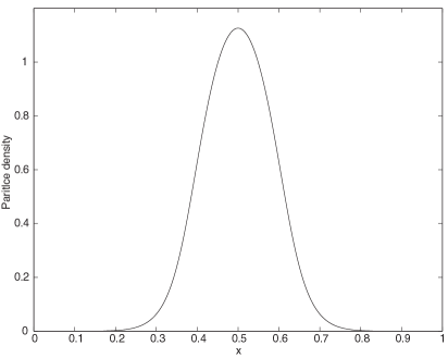
(a) Particle density $\rho_{\mathrm{ref}}$

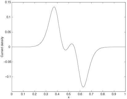
(b) Current density ${\mathbf{j}}_{\mathrm{ref}}$

Figure 1. Particle and current densities at time $T^{*}=0.05$ and for $\varepsilon=10^{-4}$.

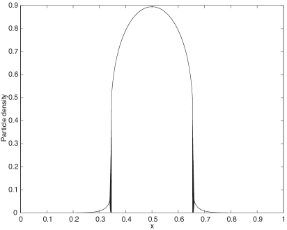
(a) Particle density $\rho_{\mathrm{ref}}$

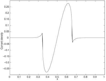
(b) Current density ${\mathbf{j}}_{\mathrm{ref}}$

Figure 2. Particle and current densities at time $T^{*}=0.13$ and for $\varepsilon=10^{-4}$.

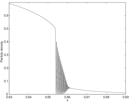
(a) Particle density $\rho_{\mathrm{ref}}$

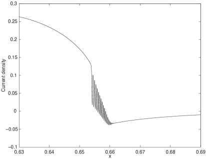
(b) Current density ${\mathbf{j}}_{\mathrm{ref}}$

Figure 3. Zoom around singularity of density and current at time $T^{*}=0.13$ and for $\varepsilon=10^{-4}$.

In order to show the asymptotic preserving property of our scheme, we compute relative $\ell^{1}$ errors at time $t_{n}$ thanks to the formula

$$\mathrm{err}_{\rho^{\varepsilon}}(t_{n})=\|\rho^{\varepsilon}_{\rm ref}-\rho^{n,\varepsilon}\|_{1}/\|\rho^{\varepsilon}_{\rm ref}\|_{1},\quad\rho^{n,\varepsilon}_{j}=|a_{j}^{n,\varepsilon}|^{2},$$

$$\mathrm{err}_{\mathbf{j}^{\varepsilon}}(t_{n})=\|\mathbf{j}^{\varepsilon}_{\rm ref}-\mathbf{j}^{n,\varepsilon}\|_{1}/\|\mathbf{j}^{\varepsilon}_{\rm ref}\|_{1},\quad\mathbf{j}^{n,\varepsilon}_{j}=\varepsilon\operatorname{Im}(\overline{a_{j}^{n,\varepsilon}}\nabla a^{n,\varepsilon}_{j})+\rho^{n,\varepsilon}_{j}v^{n,\varepsilon}_{j},$$

where the $\ell^{1}$ norm is

$$\|u\|_{1}=\Delta x\sum_{k=1}^{J-1}|u_{j}|.$$

We evaluate the error function for different values of $J=2^{M}$, where $M$ is an integer here chosen in $[4,13]$, and various scaled Planck parameter $\varepsilon$ in $[10^{-4},10^{0}]$. We plot on Figures 4, 5, 6 and 7 the relative error on physical observables $\rho^{\varepsilon}$ and $\mathbf{j}^{\varepsilon}$ computed with our AP schemes at time $t=0.05$ and $t=0.13$ respectively before and after the formation of singularities. We clearly see that the error is proportional to $(\Delta x)^{2}$, independently of $\varepsilon$ before formation of singularities. Indeed, the mean slope of the error curves with respect to $\Delta x$ is close to the value $2$ (subfigures (a)). The independence with respect to $\varepsilon$ appears in subfigures (b) where error curves are flat. After the formation of shocks, the behavior of our scheme is very different and the mesh parameters have to be reduced as $\varepsilon\to 0$ to get good accuracy.

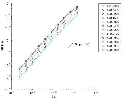
(a) Error w.r.t $J=2^{M}$

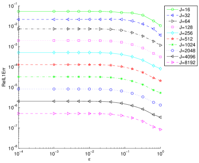
(b) Error w.r.t $\varepsilon$

Figure 4. $\mathrm{err}_{\rho^{\varepsilon}}(t=0.05)$ for AP scheme

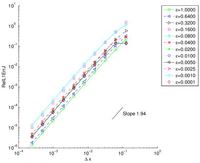
(a) Error w.r.t $J=2^{M}$

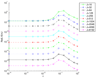
(b) Error w.r.t $\varepsilon$

Figure 5. $\mathrm{err}_{\mathbf{j}^{\varepsilon}}(t=0.05)$ for AP scheme

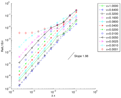
(a) Error w.r.t $J=2^{M}$

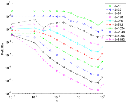
(b) Error w.r.t $\varepsilon$

Figure 6. $\mathrm{err}_{\rho^{\varepsilon}}(t=0.13)$ for AP scheme

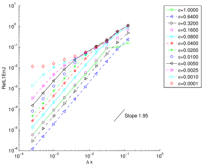
(a) Error w.r.t $J=2^{M}$

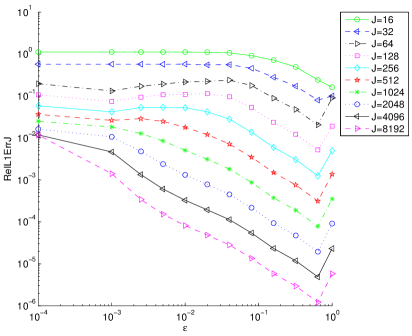
(b) Error w.r.t $\varepsilon$

Figure 7. $\mathrm{err}_{\mathbf{j}^{\varepsilon}}(t=0.13)$ for AP scheme

For a comparison, we present the same study for the classical time splitting scheme applied to (1.1)-(1.2) on Figures 8, 9, 10, 11. Thanks to the spectral accuracy of Fast Fourier Transform, the error levels are smaller than for our AP scheme which is only second order with respect to time and space variables. However, contrary to our AP scheme, the error curves clearly depend on $\varepsilon$, the error being of order $\mathcal{O}(1)$ when $\varepsilon$ is smaller than $2.10^{-3}$. In order to have good accuracy, it is required to take $\Delta x\lesssim\varepsilon$.

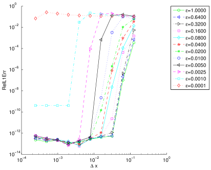
(a) Error w.r.t $J=2^{M}$

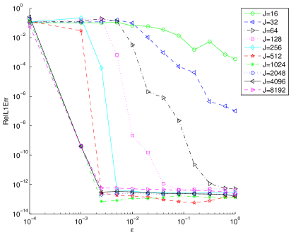
(b) Error w.r.t $\varepsilon$

Figure 8. $\mathrm{err}_{\rho^{\varepsilon}}(t=0.05)$ for time splitting scheme

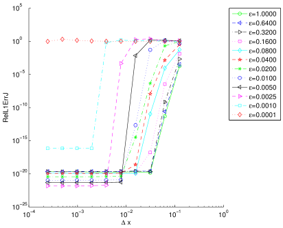
(a) Error w.r.t $J=2^{M}$

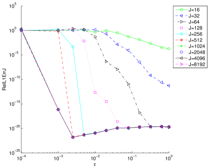
(b) Error w.r.t $\varepsilon$

Figure 9. $\mathrm{err}_{\mathbf{j}^{\varepsilon}}(t=0.05)$ for time splitting scheme

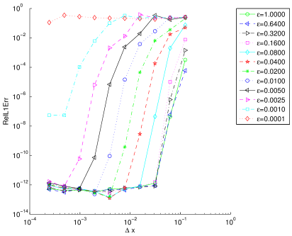
(a) Error w.r.t $J=2^{M}$

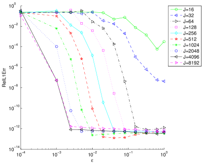
(b) Error w.r.t $\varepsilon$

Figure 10. $\mathrm{err}_{\rho^{\varepsilon}}(t=0.13)$ for time splitting scheme

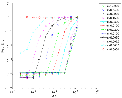
(a) Error w.r.t $J=2^{M}$

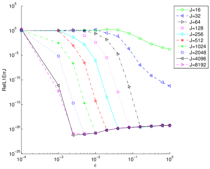
(b) Error w.r.t $\varepsilon$

Figure 11. $\mathrm{err}_{\mathbf{j}^{\varepsilon}}(t=0.13)$ for time splitting scheme

To make our presentation complete, we present the reconstruction of $u^{\varepsilon}$ thanks to equation (1.14) with $\varepsilon=0.005$. We therefore compute the phase $\phi^{\varepsilon}$ with amplitude $a^{\varepsilon}$ and velocity $v^{\varepsilon}$. Since we have access to values of these quantities at every discrete time $t_{n}$, we approximate the time dependent integral thank to a simple rectangular quadrature. We see that we can recover a very good approximation of the wave function $u^{\varepsilon}$ with very few points before the formation of singularities (see Fig. 12). Obviously, one needs more points to have a good reconstruction of the wave function passed the singularities (see Figs. 13 and 14).

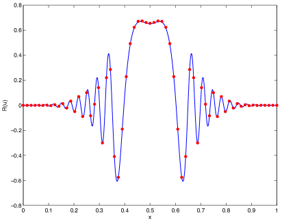
(a) $J=128$

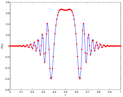
(b) $J=256$

Figure 12. $\text{Re}(u^{\varepsilon})$ at $T=0.05$ for $\varepsilon=0.005$

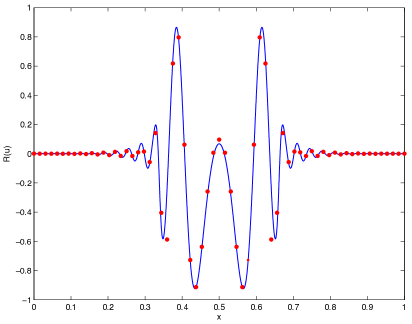
(a) $J=128$

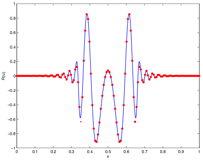
(b) $J=256$

Figure 13. $\text{Re}(u^{\varepsilon})$ at $T=0.13$ for $\varepsilon=0.005$

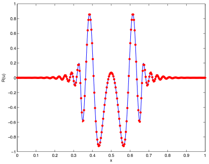
(a) $J=512$

Figure 14. $\text{Re}(u^{\varepsilon})$ at $T=0.13$ for $\varepsilon=0.005$

3.3. Numerical experiments in dimension 2

The previous subsection was devoted to one dimensional simulations. We present here the equivalent error analysis for the two dimensional case. The computational domain is now the square $[-0.5,1.5]^{2}$ discretized with $J$ points in each direction. We still need a reference solution generated with Strang splitting scheme applied to equation (1.1)-(1.2). We take $J_{\text{ref}}=2^{13}=8192$, so $\Delta x\sim 2.5\,10^{-4}$ and $\Delta t=\varepsilon/100$. In a first test, the initial datum is related to the one chosen for the one dimensional case

$$\begin{array}[]{l}\displaystyle a_{0}(x,y)=e^{-25\,r^{2}},\\[5.69054pt] \displaystyle v_{0}(x)=-\frac{1}{5}\nabla\ln{(e^{5\,r}+e^{-5\,r})}.\end{array}$$

where $r=\sqrt{(x-0.5)^{2}+(y-0.5)^{2}}$. We evaluate the error function for different values of $J=2^{M}$, where $M$ is chosen in $[4,11]$, and various scaled Planck parameter $\varepsilon$ in $[5.10^{-4},10^{0}]$. The formation time of singularities is as in one dimension situation located around $0.10$. The reference particle and current densities for $\varepsilon=5.10^{-4}$ are represented on Figures 15 and 17 before and after formation of singularities. We clearly see that a tiny front appears after shocks both in particle and current densities. The wave function presents strong oscillations with new ones created past the shock creation (see Fig. 17)

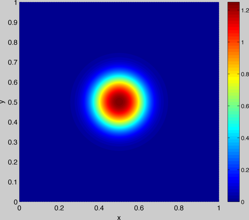
(a) $\rho_{\mathrm{ref}}$

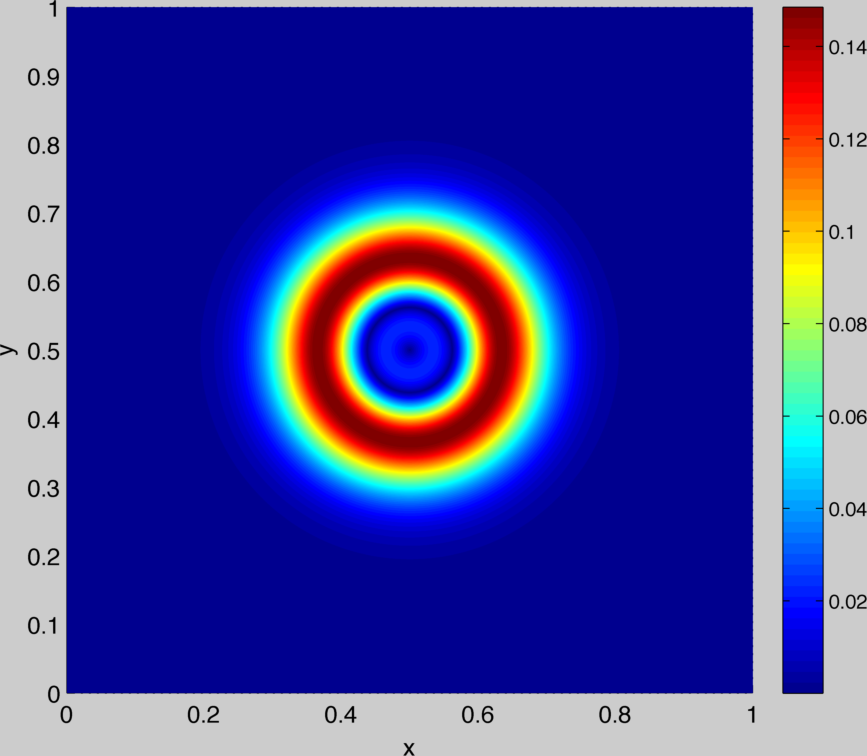
(b) $\mathbf{j}_{\mathrm{ref}}$

Figure 15. Contour plot of particle and current densities at time $t=0.05$ and for $\varepsilon=5.10^{-4}$

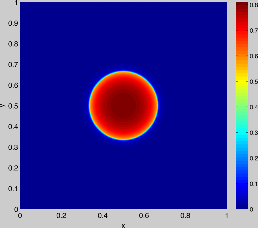
(a) $\rho_{\mathrm{ref}}$

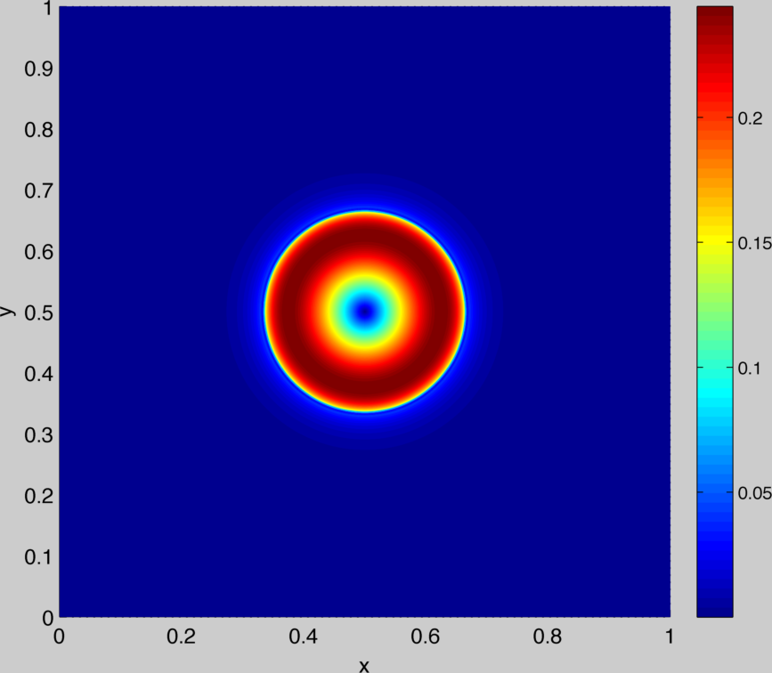
(b) $\mathbf{j}_{\mathrm{ref}}$

Figure 16. Contour plot of particle and current densities at time $t=0.13$ and for $\varepsilon=5.10^{-4}$

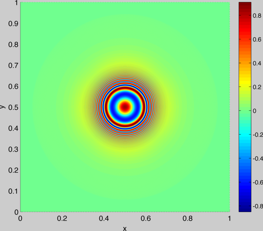
(a) $u^{\varepsilon}$ at time $t=0.05$

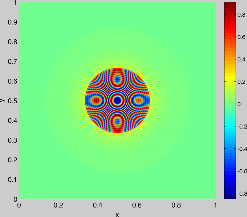
(b) $u^{\varepsilon}$ at time $t=0.13$

Figure 17. Contour plot of real part of $u^{\varepsilon}$ at times $t=0.05$ and $t=0.13$ and for $\varepsilon=5.10^{-4}$

The error analysis results are equivalent to the ones obtained for one dimensional simulation. We recover an independence of the error with respect to $\varepsilon$ before the formation of singularities (see Figs 18 and 19). We always need to take finer mesh past the shocks formation (see Figs 20 and 21).

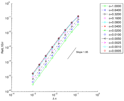
(a) Error w.r.t $J=2^{M}$

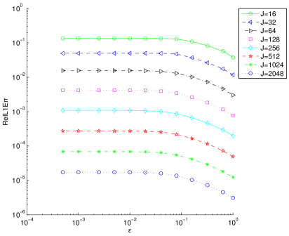
(b) Error w.r.t $\varepsilon$

Figure 18. $\mathrm{err}_{\rho^{\varepsilon}}(t=0.05)$ for AP scheme

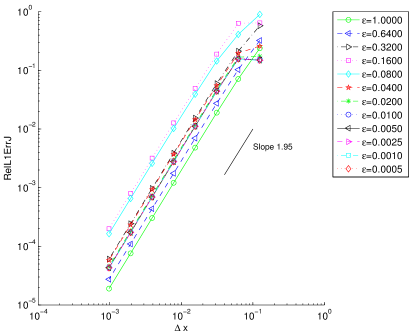
(a) Error w.r.t $J=2^{M}$

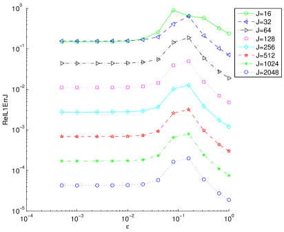
(b) Error w.r.t $\varepsilon$

Figure 19. $\mathrm{err}_{\mathbf{j}^{\varepsilon}}(t=0.05)$ for AP scheme

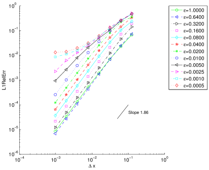
(a) Error w.r.t $J=2^{M}$

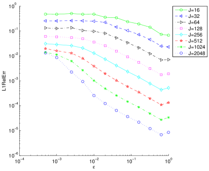
(b) Error w.r.t $\varepsilon$

Figure 20. $\mathrm{err}_{\rho^{\varepsilon}}(t=0.13)$ for AP scheme

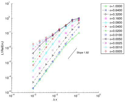
(a) Error w.r.t $J=2^{M}$

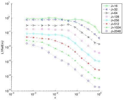
(b) Error w.r.t $\varepsilon$

Figure 21. $\mathrm{err}_{\mathbf{j}^{\varepsilon}}(t=0.13)$ for AP scheme

The last computation concerns a non-symmetric solution. The aim of our simulations is to show that we recover good qualitative properties, even for non radially symmetric data. We consider here as initial datum a Maxwell distribution with two temperatures $\theta_{1}=0.05$ and $\theta_{2}=0.015$ for the initial amplitude given by

$$a_{0}=\frac{1}{\sqrt{4}}\frac{1}{2\pi\sqrt{\theta_{1}}\sqrt{\theta_{2}}}\exp{\left({-\frac{(x-0.5)^{2}}{2\theta_{1}}-\frac{(y-0.5)^{2}}{2\theta_{2}}}\right)}.$$

The initial phase is reduced to $\phi_{0}=0$ (note that from (1.11), ${\partial}_{t}\phi_{\mid t=0}=-|a_{0}|^{2}\not=0$, so $\phi$ becomes instantaneously non-trivial). The scaled Planck factor $\varepsilon$ is equal to $\varepsilon=0.005$ and the simulations are performed with $J=2048$ intervals in each direction. To distinguish the evolution for each direction $(x,y)$, we make contour plots of wave function and physical observables but also present slice for plane $x=0.5$ and $y=0.5$ respectively on bottom right and upper right axes. The solution has many oscillations in both directions before formation of singularities (see the real part of the wave function $u^{\varepsilon}$ on Fig. 22 at time $t=0.035$). The oscillatory nature is enhanced at time $t=0.08$ mainly in $y-$direction (see Fig. 23).

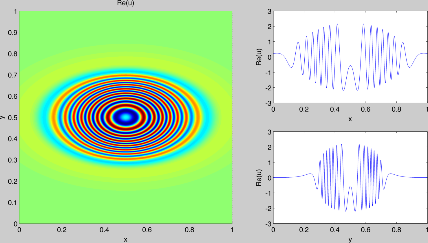
Figure 22. $\text{Re}(u^{\varepsilon})(t=0.035)$

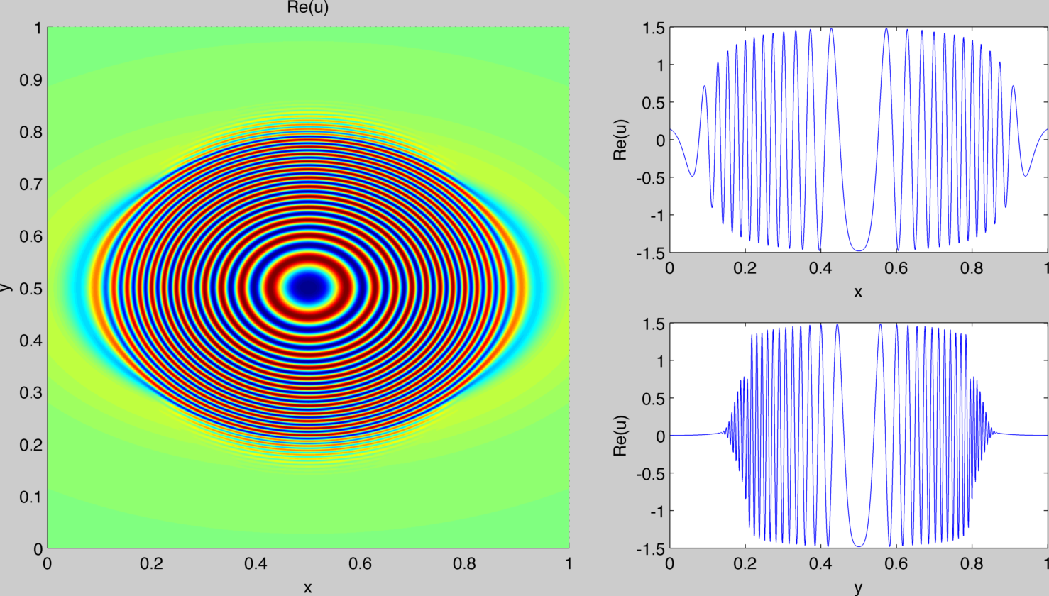
Figure 23. $\text{Re}(u^{\varepsilon})(t=0.08)$

We recover the good behavior of physical observables before the formation time of singularities. Actually, we compare the particle densities computed by Strang splitting scheme and our AP scheme at time $t=0.035$ on Figures 24 and 25. The similar representation for $\mathbf{j}^{\varepsilon}$ is available on Figures 28 and 29. Past the formation time of singularities, the contour plots could be thought as equivalent both for particle and current densities. The only noticeable differences can be seen on $x=0.5$ and $y=0.5$ plane slices (see Fig. 26, 27, 30 and 31).

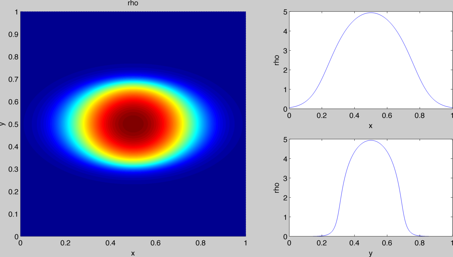
Figure 24. Strang $\rho^{\varepsilon}(t=0.035)$

Figure 25. AP $\rho^{\varepsilon}(t=0.035)$

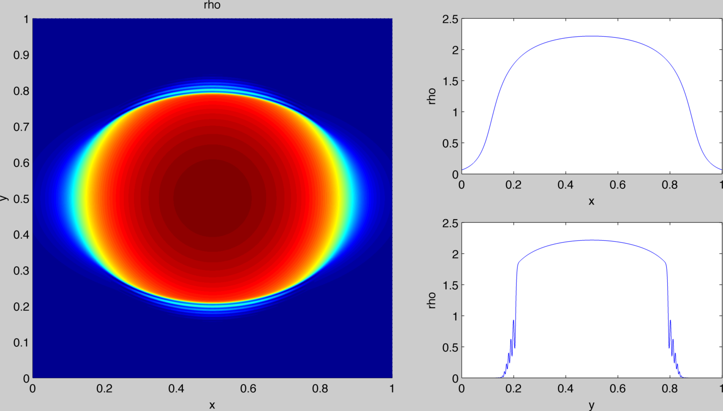
Figure 26. Strang $\rho^{\varepsilon}(t=0.08)$

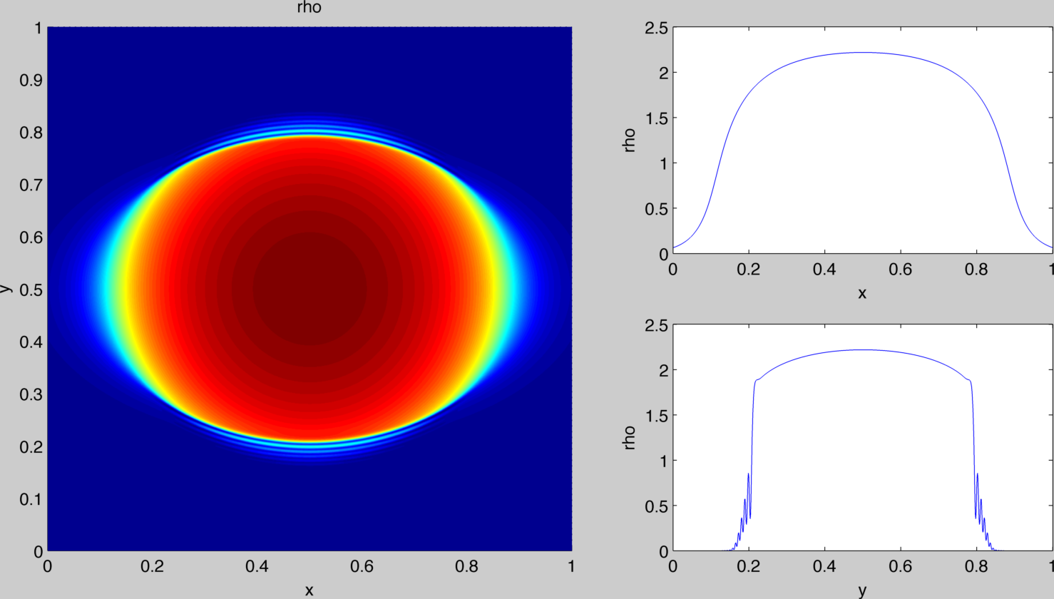
Figure 27. AP $\rho^{\varepsilon}(t=0.08)$

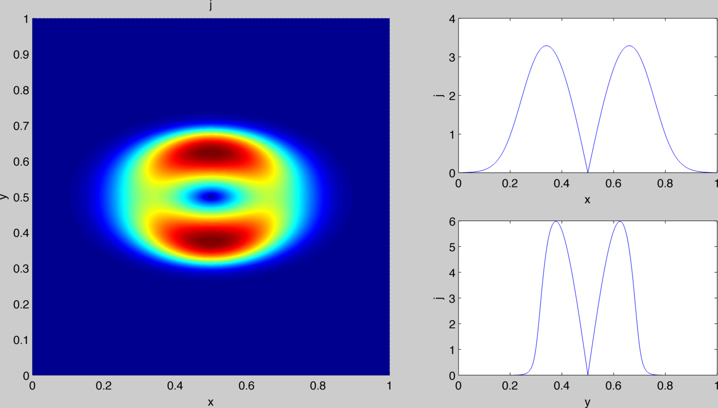
Figure 28. Strang ${\mathbf{j}}^{\varepsilon}(t=0.035)$

Figure 29. AP ${\mathbf{j}}^{\varepsilon}(t=0.035)$

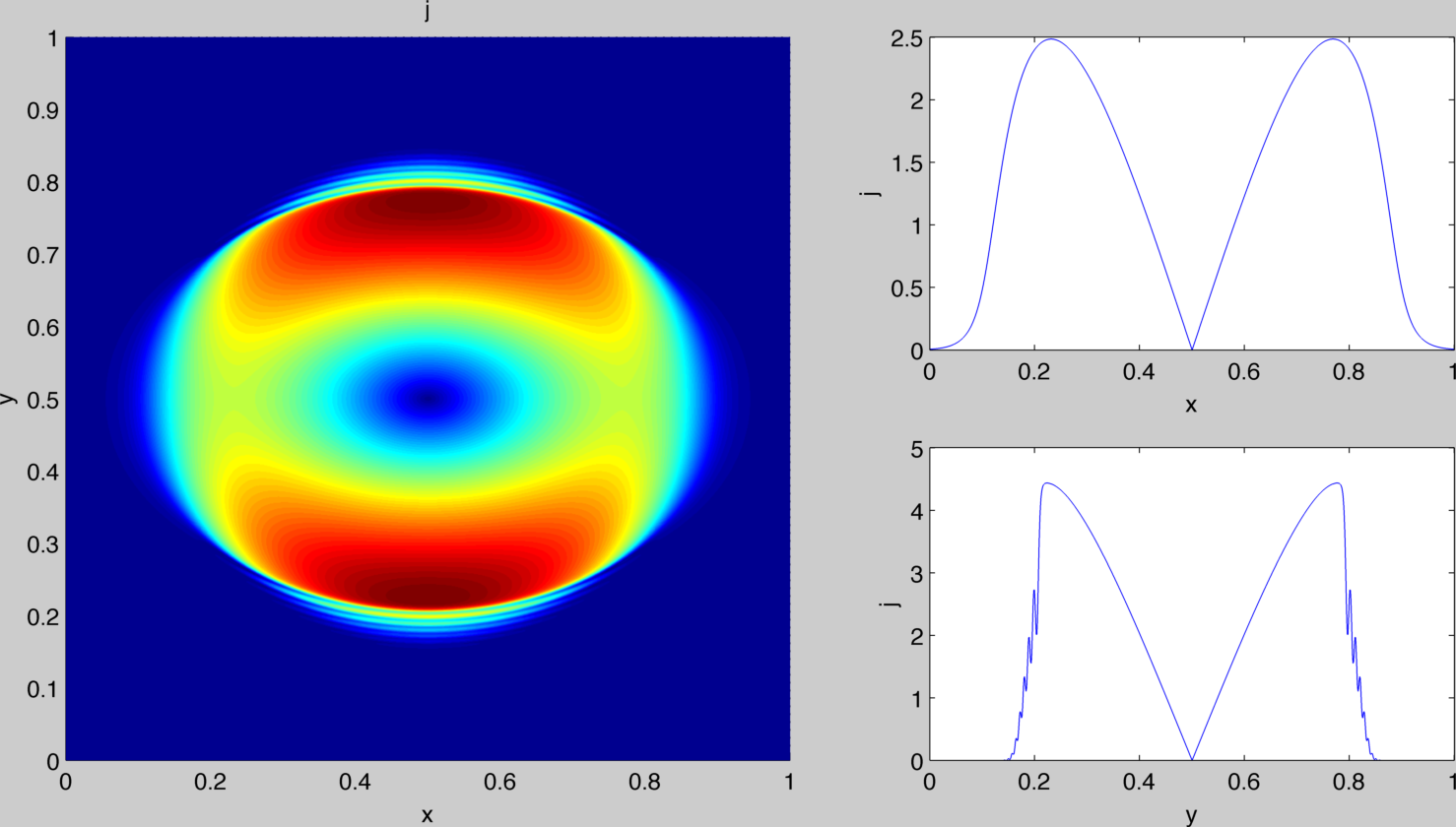
Figure 30. Strang ${\mathbf{j}}^{\varepsilon}(t=0.08)$

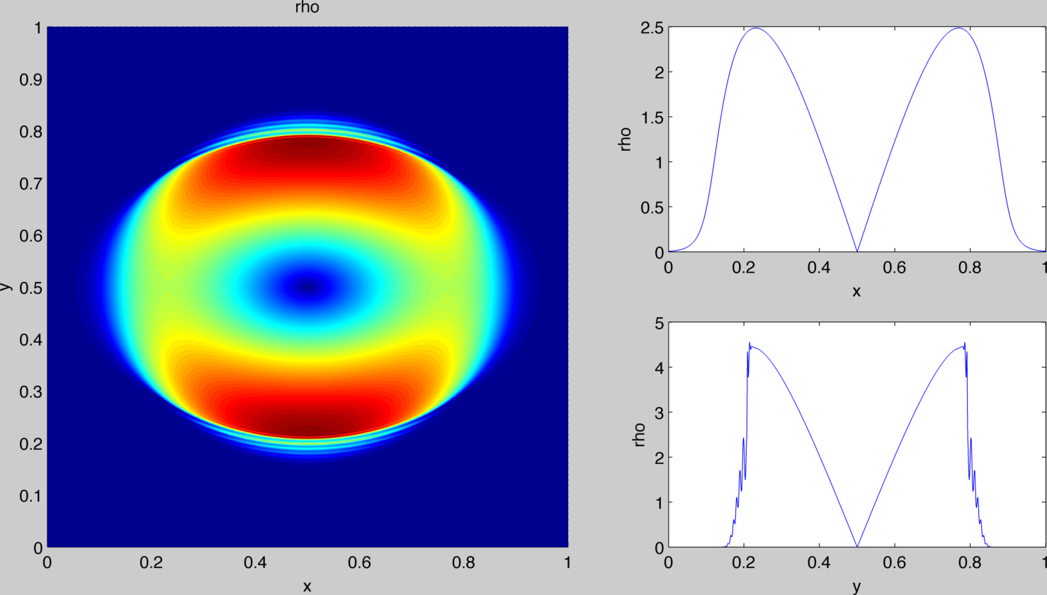
Figure 31. AP ${\mathbf{j}}^{\varepsilon}(t=0.08)$

4. Extension to other frameworks

4.1. The linear case: global solution of the viscous eikonal equation

The advantage of introducing an artificial diffusion is more striking in the linear case. Consider

$$i\varepsilon{\partial}_{t}u^{\varepsilon}+\frac{\varepsilon^{2}}{2}\Delta u^{\varepsilon}=V_{\rm ext}u^{\varepsilon};\quad u^{\varepsilon}_{\mid t=0}=a_{0}e^{i\phi_{0}/\varepsilon},$$ (4.1)

with $V_{\rm ext}=V_{\rm ext}(t,x)$ real-valued. As noticed in [22], using the Madelung transform in this context is interesting only if vacuum can be avoided. Having the idea of Grenier [29] in mind, the counterpart of (1.8) reads

$$\left\{\begin{aligned} &{\partial}_{t}a^{\varepsilon}+\nabla\phi^{\varepsilon}\cdot\nabla a^{\varepsilon}+\frac{1}{2}a^{\varepsilon}\Delta\phi^{\varepsilon}=i\frac{\varepsilon}{2}\Delta a^{\varepsilon},\qquad&&a^{\varepsilon}_{\mid t=0}=a_{0},\\ &{\partial}_{t}\phi^{\varepsilon}+\frac{1}{2}|\nabla\phi^{\varepsilon}|^{2}+V_{\rm ext}=0,\qquad&&\phi^{\varepsilon}_{\mid t=0}=\phi_{0}.\end{aligned}\right.$$

We note that the two equations are decoupled: the second equation is of Hamilton-Jacobi type (known as the eikonal equation in this context), and the solution must be expected to develop singularities in finite time (see e.g. [12]), so this approach is doomed to fail for large time. On the other hand, introducing the artificial diffusion as in (1.11), we obtain

$$\left\{\begin{aligned} &{\partial}_{t}a^{\varepsilon}+\nabla\phi^{\varepsilon}\cdot\nabla a^{\varepsilon}+\frac{1}{2}a^{\varepsilon}\Delta\phi^{\varepsilon}=i\frac{\varepsilon}{2}\Delta a^{\varepsilon}-i\varepsilon a^{\varepsilon}\Delta\phi^{\varepsilon},\qquad&&a^{\varepsilon}_{\mid t=0}=a_{0},\\ &{\partial}_{t}\phi^{\varepsilon}+\frac{1}{2}|\nabla\phi^{\varepsilon}|^{2}+V_{\rm ext}=\varepsilon^{2}\Delta\phi^{\varepsilon},\qquad&&\phi^{\varepsilon}_{\mid t=0}=\phi_{0}.\end{aligned}\right.$$ (4.2)

The system is still decoupled, but the good news is that the diffusion introduced into the Hamilton-Jacobi equation smoothes the solution out. Therefore, this system can be considered as a good candidate to obtain an AP scheme for the linear Schrödinger equation, regardless of the presence of vacuum.

Instead of giving full details of the analogue of Theorems 1.4, 1.6 and 1.7, as well as of their proofs, we shall simply give a functional framework where the viscous eikonal equation can by solved globally in time. Since we consider the case $\varepsilon>0$ only, we drop out the $\varepsilon^{2}$ term in the viscous eikonal equation, and consider

$${\partial}_{t}\phi_{\rm eik}+\frac{1}{2}|\nabla\phi_{\rm eik}|^{2}+V_{\rm ext}=\Delta\phi_{\rm eik};\quad\phi_{\rm eik}(0,x)=\phi_{0}(x).$$ (4.3)

For $k\geqslant 1$, let

$${\tt SL}_{k}=\{f\in C^{k}({\mathbb{R}}^{d};{\mathbb{R}}),\quad{\partial}^{\alpha}f\in L^{\infty}({\mathbb{R}}^{d}),\ \forall 1\leqslant|\alpha|\leqslant k\}.$$

For $k\geqslant 2$, let

$${\tt SQ}_{k}=\{f\in C^{k}({\mathbb{R}}^{d};{\mathbb{R}}),\quad{\partial}^{\alpha}f\in L^{\infty}({\mathbb{R}}^{d}),\ \forall 2\leqslant|\alpha|\leqslant k\}.$$

The key result is the following:

Lemma 4.1.

Let $k\geqslant 2$ and $\phi_{0}\in{\tt SL_{k}}$, $V_{\rm ext}\in L^{\infty}_{\rm loc}({\mathbb{R}}_{+};{\tt SL}_{k})$. Then (4.3) has a unique solution $\phi_{\rm eik}\in C({\mathbb{R}}_{+};{\tt SL}_{k-1})$.

Remark 4.2.

No such global result must be expected in the larger class ${\tt SQ}_{k}$. Indeed, suppose $d=1$, $V_{\rm ext}=0$ and $\phi_{0}(x)=-x^{2}/2$. If (4.3) had a solution $\phi_{\rm eik}\in C({\mathbb{R}}_{+};{\tt QL}_{2})$, then $w={\partial}_{x}^{2}\phi_{\rm eik}\in C({\mathbb{R}}_{+};L^{\infty})$ would solve

$${\partial}_{t}w+v{\partial}_{x}w+w^{2}={\partial}_{x}^{2}w;\quad w(0,x)=-1.$$

The solution of this equation does not depend on $x$. It is given by $w(t,x)=1/(t-1)$, hence a contradiction. However, in the periodic case $x\in{\mathbb{T}}^{d}$, this technical issue disappears (see Remark 4.3 below).

Proof.

The first step consists in constructing the gradient of $\phi_{\rm eik}$. Differentiating (4.3) in space, we have to solve

$${\partial}_{t}v+v\cdot\nabla v+\nabla V_{\rm ext}=\Delta v;\quad v(0,x)=\nabla\phi_{0}(x).$$ (4.4)

This equation is solved locally in time by a fixed point argument by using Duhamel’s formula

$$v(t)=e^{t\Delta}\nabla\phi_{0}-\int_{0}^{t}e^{(t-s)\Delta}(v\cdot\nabla v)(s)ds-\int_{0}^{t}e^{(t-s)\Delta}(\nabla V_{\rm ext})(s)ds.$$

The right hand side is a contraction on

$$\left\{w\in C\left([0,T];W^{k-1,\infty}\right),\quad\|w\|_{L^{\infty}([0,T];W^{k-1,\infty})}\leqslant 2\|\nabla\phi_{0}\|_{W^{k-1,\infty}}\right\},$$

provided that $T>0$ is sufficiently small. This follows from the properties of the heat kernel: for $t>0$,

$$\|e^{t\Delta}f\|_{L^{\infty}}\leqslant\|f\|_{L^{\infty}};\quad\|e^{t\Delta}\nabla f\|_{L^{\infty}}\leqslant\frac{C}{\sqrt{t}}\|f\|_{L^{\infty}}.$$

The solution to (4.4) is then global, thanks to the maximum principle (see e.g. [47, Proposition 52.8], which implies that $v_{-}\leqslant v\leqslant v_{+}$, where

$${\partial}_{t}v_{\pm}\mp\|\nabla V_{\rm ext}\|_{L^{\infty}_{x}}=0;\quad v_{\pm}(0,x)=\pm\|\nabla\phi_{0}\|_{L^{\infty}}.$$

Once such a solution $v\in C({\mathbb{R}}_{+};W^{k-1,\infty})$ is constructed, set

$$\phi_{\rm eik}(t)=\phi_{0}-\int_{0}^{t}\left(\frac{1}{2}|v(s)|^{2}+V_{\rm ext}(s)-\operatorname{div}v(s)\right)ds.$$

We check that ${\partial}_{t}(\nabla\phi_{\rm eik}-v)=\nabla{\partial}_{t}\phi_{\rm eik}-{\partial}_{t}v=0$. Therefore, $v=\nabla\phi_{\rm eik}$, and $\phi_{\rm eik}$ solves (4.3). Rewriting (4.3) as

$${\partial}_{t}\phi_{\rm eik}+\frac{1}{2}|v|^{2}+V_{\rm ext}=\Delta\phi_{\rm eik};\quad\phi_{\rm eik}(0,x)=\phi_{0}(x),$$

Duhamel’s formula reads

$$\phi_{\rm eik}(t)=e^{t\Delta}\phi_{0}-\int_{0}^{t}e^{(t-s)\Delta}(|v(s)|^{2})ds-\int_{0}^{t}e^{(t-s)\Delta}V_{\rm ext}(s)ds,$$

from which we conclude that $\phi_{\rm eik}\in C({\mathbb{R}}_{+};{\tt SL}_{k-1})$. ∎

Remark 4.3.

In the periodic setting $x\in{\mathbb{T}}^{d}=({\mathbb{R}}/(2\pi{\mathbb{Z}}))^{d}$, it is natural to work in the Wiener algebra

$$W=\left\{f:{\mathbb{T}}^{d}\to{\mathbb{C}},\quad f(x)=\sum_{j\in{\mathbb{Z}}^{d}}b_{j}e^{ij\cdot x}\text{ with }(b_{j})_{j\in{\mathbb{Z}}^{d}}\in\ell^{1}({\mathbb{Z}}^{d})\right\},$$

and for $k\geqslant 0$,

$$W^{k}=\{f:{\mathbb{T}}^{d}\to{\mathbb{C}},\quad{\partial}^{\alpha}f\in W,\ \forall|\alpha|\leqslant k\}.$$

Then Lemma 4.1 is easily adapted by replacing ${\tt SL}_{k}$ with $W^{k}$.

4.2. Other nonlinearities

One might believe that Theorem 1.7 is bound to the cubic one-dimensional Schrödinger equation, which is completely integrable, and that the two aspects are related. We show that this is not the case, since Theorem 1.7 remains valid for other nonlinearities (with $d=1$). Consider now

$$i\varepsilon{\partial}_{t}u^{\varepsilon}+\frac{\varepsilon^{2}}{2}\Delta u^{\varepsilon}=f\left(|u^{\varepsilon}|^{2}\right)u^{\varepsilon},\quad(t,x)\in{\mathbb{R}}_{+}\times{\mathbb{R}}^{d}.$$ (4.5)

We suppose that there exists $\delta>0$ such that $f^{\prime}(y)\geqslant\delta$, for all $y\geqslant 0$.

Following [29], the only modification we have to make to recover the results in Section 2.1 consists in replacing the symmetrizer (2.2) with

$$S=\begin{pmatrix}I_{2}&0\\ 0&\frac{1}{4f^{\prime}(a_{1}^{2}+a_{2}^{2})}I_{d}\end{pmatrix}.$$

From our assumption on $f$, $S$ and its inverse $S^{-1}$ are uniformly bounded, provided that $a$ is bounded. As a matter of fact, the exact assumption in [29] is $f^{\prime}>0$, and all the results in Section 2.1 remain valid under this assumption.

The more precise assumption $f^{\prime}(y)\geqslant\delta$ becomes useful to prove that in dimension $d=1$, the solution is global. The main point to notice is that the conservation of mass and momentum are the same as for (1.1), like in Proposition 1.1. On the other hand, the conservation of energy becomes

$$\frac{d}{dt}\left(\|\varepsilon\nabla u^{\varepsilon}(t)\|_{L^{2}}^{2}+\int_{{\mathbb{R}}^{d}}F\left(|u^{\varepsilon}(t,x)|^{2}\right)dx\right)=0,$$

where $F$ is an anti-derivative of $f$,

$$F(y)=\int_{0}^{y}f(r)dr.$$

By assumption,

$$F(y)\geqslant\frac{\delta}{2}y^{2}+f(0)y,$$

so the potential energy controls the $L^{4}$-norm:

$$\|u^{\varepsilon}(t)\|_{L^{4}}^{4} \leqslant\frac{2}{\delta}\left(\int_{{\mathbb{R}}^{d}}F\left(|u^{\varepsilon}(t,x)|^{2}\right)dx-f(0)\|u^{\varepsilon}(t)\|_{L^{2}}^{2}\right)$$

$$\leqslant\frac{2}{\delta}\left(\int_{{\mathbb{R}}^{d}}F\left(|u^{\varepsilon}(t,x)|^{2}\right)dx-f(0)\|u^{\varepsilon}(0)\|_{L^{2}}^{2}\right),$$

where we have used the conservation of mass in the last inequality. This implies an estimate of the form

$$\|\varepsilon\nabla u^{\varepsilon}(t)\|_{L^{2}}^{2}+\|u^{\varepsilon}(t)\|_{L^{4}}^{4}\leqslant C,$$

with $C$ independent of $t\geqslant 0$ and $\varepsilon\in(0,1]$. Therefore, the analysis presented in Section 2.3 can be repeated line by line.

Example 4.4.

The assumption $f^{\prime}\geqslant\delta>0$ is satisfied in the following cases:

• Cubic-quintic nonlinearity: $f(y)=y+\lambda y^{2}$, $\lambda\geqslant 0$.

• Cubic plus saturated nonlinearity: $f(y)=\delta y+\eta\frac{y}{1+\lambda y}$, $\delta,\eta,\lambda>0$.

Acknowledgements

C. Besse was partially supported by the French ANR fundings under the project MicroWave NT09_460489. R. Carles was supported by the French ANR project R.A.S. (ANR-08-JCJC-0124-01). C. Besse and F. Méhats were partially supported by the ANR-FWF Project Lodiquas (ANR-11-IS01-0003).

References

- [1] G. D. Akrivis, Finite difference discretization of the cubic Schrödinger equation, IMA J. Numer. Anal., 13 (1993), pp. 115–124.
- [2] T. Alazard and R. Carles, Loss of regularity for super-critical nonlinear Schrödinger equations, Math. Ann., 343 (2009), pp. 397–420.
- [3] A. Arnold, N. Ben Abdallah, and C. Negulescu, WKB-based schemes for the oscillatory 1D Schrödinger equation in the semiclassical limit, SIAM J. Numer. Anal., 49 (2011), pp. 1436–1460.
- [4] H. Bahouri, J.-Y. Chemin, and R. Danchin, Fourier analysis and nonlinear partial differential equations, vol. 343 of Grundlehren der Mathematischen Wissenschaften [Fundamental Principles of Mathematical Sciences], Springer, Heidelberg, 2011.
- [5] W. Bao, S. Jin, and P. A. Markowich, On time-splitting spectral approximations for the schrödinger equation in the semiclassical regime, Journal of Comp. Phys., 175 (2002), pp. 487–524.
- [6] , Numerical study of time-splitting spectral discretizations of nonlinear Schrödinger equations in the semiclassical regimes, SIAM J. Sci. Comput., 25 (2003), pp. 27–64.
- [7] M. Bennoune, M. Lemou, and L. Mieussens, Uniformly stable numerical schemes for the Boltzmann equation preserving the compressible Navier-Stokes asymptotics, J. Comput. Phys., 227 (2008), pp. 3781–3803.
- [8] C. Besse, A relaxation scheme for the nonlinear Schrödinger equation, SIAM J. Numer. Anal., 42 (2004), pp. 934–952 (electronic).
- [9] C. Besse, B. Bidégaray, and S. Descombes, Order estimates in time of splitting methods for the nonlinear Schrödinger equation, SIAM J. Numer. Anal., 40 (2002), pp. 26–40 (electronic).
- [10] Y. Brenier, Convergence of the Vlasov-Poisson system to the incompressible Euler equations, Comm. Partial Differential Equations, 25 (2000), pp. 737–754.
- [11] C. Buet and B. Despres, Asymptotic preserving and positive schemes for radiation hydrodynamics, J. Comput. Phys., 215 (2006), pp. 717–740.
- [12] R. Carles, Semi-classical analysis for nonlinear Schrödinger equations, World Scientific Publishing Co. Pte. Ltd., Hackensack, NJ, 2008.
- [13] R. Carles, R. Danchin, and J.-C. Saut, Madelung, Gross-Pitaevskii and Korteweg, Nonlinearity, 25 (2012), pp. 2843–2873.
- [14] R. Carles, C. Fermanian Kammerer, N. J. Mauser, and H. P. Stimming, On the time evolution of Wigner measures for Schrödinger equations, Commun. Pure Appl. Anal., 8 (2009), pp. 559–585.
- [15] R. Carles and B. Mohammadi, Numerical aspects of the nonlinear Schrödinger equation in the semiclassical limit in a supercritical regime, ESAIM Math. Model. Numer. Anal., 45 (2011), pp. 981–1008.
- [16] J. A. Carrillo, T. Goudon, P. Lafitte, and F. Vecil, Numerical schemes of diffusion asymptotics and moment closures for kinetic equations, J. Sci. Comput., 36 (2008), pp. 113–149.
- [17] T. Cazenave, Semilinear Schrödinger equations, vol. 10 of Courant Lecture Notes in Mathematics, New York University Courant Institute of Mathematical Sciences, New York, 2003.
- [18] J.-Y. Chemin, Dynamique des gaz à masse totale finie, Asymptotic Anal., 3 (1990), pp. 215–220.
- [19] F. Coron and B. Perthame, Numerical passage from kinetic to fluid equations, SIAM J. Numer. Anal., 28 (1991), pp. 26–42.
- [20] P. Crispel, P. Degond, and M.-H. Vignal, An asymptotic preserving scheme for the two-fluid Euler-Poisson model in the quasineutral limit, J. Comput. Phys., 223 (2007), pp. 208–234.
- [21] P. Degond, F. Deluzet, L. Navoret, A.-B. Sun, and M.-H. Vignal, Asymptotic-preserving particle-in-cell method for the Vlasov-Poisson system near quasineutrality, J. Comput. Phys., 229 (2010), pp. 5630–5652.
- [22] P. Degond, S. Gallego, and F. Méhats, An asymptotic preserving scheme for the Schrödinger equation in the semiclassical limit, C. R. Math. Acad. Sci. Paris, 345 (2007), pp. 531–536.
- [23] P. Degond, A. Lozinski, J. Narski, and C. Negulescu, An asymptotic-preserving method for highly anisotropic elliptic equations based on a micro-macro decomposition, J. Comput. Phys., 231 (2012), pp. 2724–2740.
- [24] M. Delfour, M. Fortin, and G. Payre, Finite-difference solutions of a nonlinear Schrödinger equation, J. Comput. Phys., 44 (1981), pp. 277–288.
- [25] F. Filbet and S. Jin, A class of asymptotic-preserving schemes for kinetic equations and related problems with stiff sources, J. Comput. Phys., 229 (2010), pp. 7625–7648.
- [26] E. Gabetta, L. Pareschi, and G. Toscani, Relaxation schemes for nonlinear kinetic equations, SIAM J. Numer. Anal., 34 (1997), pp. 2168–2194.
- [27] P. Gérard, P. A. Markowich, N. J. Mauser, and F. Poupaud, Homogenization limits and Wigner transforms, Comm. Pure Appl. Math., 50 (1997), pp. 323–379.
- [28] L. Gosse and G. Toscani, Asymptotic-preserving & well-balanced schemes for radiative transfer and the Rosseland approximation, Numer. Math., 98 (2004), pp. 223–250.
- [29] E. Grenier, Semiclassical limit of the nonlinear Schrödinger equation in small time, Proc. Amer. Math. Soc., 126 (1998), pp. 523–530.
- [30] H. Holden, C. Lubich, and N. H. Risebro, Operator splitting for partial differential equations with Burgers nonlinearity, Math. Comp., 82 (2013), pp. 173–185.
- [31] S. Jin, Efficient asymptotic-preserving (AP) schemes for some multiscale kinetic equations, SIAM J. Sci. Comput., 21 (1999), pp. 441–454 (electronic).
- [32] S. Jin, P. Markowich, and C. Sparber, Mathematical and computational methods for semiclassical Schrödinger equations, Acta Numer., 20 (2011), pp. 121–209.
- [33] S. Jin, L. Pareschi, and G. Toscani, Uniformly accurate diffusive relaxation schemes for multiscale transport equations, SIAM J. Numer. Anal., 38 (2000), pp. 913–936 (electronic).
- [34] O. Karakashian, G. D. Akrivis, and V. A. Dougalis, On optimal order error estimates for the nonlinear Schrödinger equation, SIAM J. Numer. Anal., 30 (1993), pp. 377–400.
- [35] T. Kato and G. Ponce, Commutator estimates and the Euler and Navier-Stokes equations, Comm. Pure Appl. Math., 41 (1988), pp. 891–907.
- [36] A. Klar, An asymptotic-induced scheme for nonstationary transport equations in the diffusive limit, SIAM J. Numer. Anal., 35 (1998), pp. 1073–1094 (electronic).
- [37] C. Klein, Fourth order time-stepping for low dispersion Korteweg-de Vries and nonlinear Schrödinger equations, Electron. Trans. Numer. Anal., 29 (2007/08), pp. 116–135.
- [38] P. Lafitte and G. Samaey, Asymptotic-preserving projective integration schemes for kinetic equations in the diffusion limit, SIAM J. Sci. Comput., 34 (2012), pp. A579–A602.
- [39] M. Lemou and L. Mieussens, A new asymptotic preserving scheme based on micro-macro formulation for linear kinetic equations in the diffusion limit, SIAM J. Sci. Comput., 31 (2008), pp. 334–368.
- [40] F. Lin and P. Zhang, Semiclassical limit of the Gross-Pitaevskii equation in an exterior domain, Arch. Rational Mech. Anal., 179 (2006), pp. 79–107.
- [41] P.-L. Lions and T. Paul, Sur les mesures de Wigner, Rev. Mat. Iberoamericana, 9 (1993), pp. 553–618.
- [42] E. Madelung, Quanten theorie in hydrodynamischer form, Zeit. F. Physik, 40 (1927), p. 322.
- [43] T. Makino, S. Ukai, and S. Kawashima, Sur la solution à support compact de l’équation d’Euler compressible, Japan J. Appl. Math., 3 (1986), pp. 249–257.
- [44] P. A. Markowich, P. Pietra, and C. Pohl, Numerical approximation of quadratic observables of Schrödinger-type equations in the semi-classical limit, Numer. Math., 81 (1999), pp. 595–630.
- [45] P. A. Markowich, P. Pietra, C. Pohl, and H.-P. Stimming, A Wigner-measure analysis of the Dufort-Frankel scheme for the Schrödinger equation, SIAM J. Numer. Anal., 40 (2002), pp. 1281–1310.
- [46] D. Pathria and J. L. Morris, Pseudo-spectral solution of nonlinear Schrödinger equations, J. Comput. Phys., 87 (1990), pp. 108–125.
- [47] P. Quittner and P. Souplet, Superlinear parabolic problems, Birkhäuser Advanced Texts: Basler Lehrbücher. [Birkhäuser Advanced Texts: Basel Textbooks], Birkhäuser Verlag, Basel, 2007. Blow-up, global existence and steady states.
- [48] J. M. Sanz-Serna and J. G. Verwer, Conservative and nonconservative schemes for the solution of the nonlinear Schrödinger equation, IMA J. Numer. Anal., 6 (1986), pp. 25–42.
- [49] M. Taylor, Partial differential equations. III, vol. 117 of Applied Mathematical Sciences, Springer-Verlag, New York, 1997. Nonlinear equations.
- [50] J. A. C. Weideman and B. M. Herbst, Split-step methods for the solution of the nonlinear Schrödinger equation, SIAM J. Numer. Anal., 23 (1986), pp. 485–507.
- [51] L. Wu, Dufort-Frankel-type methods for linear and nonlinear Schrödinger equations, SIAM J. Numer. Anal., 33 (1996), pp. 1526–1533.
- [52] R. E. Wyatt, Quantum Dynamics with Trajectories: Introduction to Quantum Hydrodynamics, Springer, New York, 2005.
- [53] Z. Xin, Blowup of smooth solutions of the compressible Navier-Stokes equation with compact density, Comm. Pure Appl. Math., 51 (1998), pp. 229–240.
- [54] P. Zhang, Semiclassical limit of nonlinear Schrödinger equation. II, J. Partial Differential Equations, 15 (2002), pp. 83–96.
- [55] , Wigner measure and the semiclassical limit of Schrödinger-Poisson equations, SIAM J. Math. Anal., 34 (2002), pp. 700–718.