Generation of arbitrary symmetric entangled states with conditional linear optical coupling

Abstract

An approach for generating the entangled photonic states $\left|\Psi_{1},\Psi_{2}\right\rangle\pm\left|\Psi_{2},\Psi_{1}\right\rangle$ from two arbitrary states $|\Psi_{1}\rangle$ and $|\Psi_{2}\rangle$ is proposed. The protocol is implemented by the conditionally induced beam-splitter coupling which leads to the selective swapping between two photonic modes. Such coupling occurs in a quantum system prepared in the superposition of two ground states with only one of them being involved in the swapping. All the entangled states in the category, such as entangled pairs of coherent states or Fock states (N00N states), can be efficiently produced in the same way by this method.

I introduction

Bipartite symmetric entangled states refer to a generic type in the form $\left|\Psi_{1},\Psi_{2}\right\rangle\pm\left|\Psi_{2},\Psi_{1}\right\rangle$ up to a normalization factor. Such entangled states include the symmetric entangled coherent states (SECSs) $\left|\alpha,\beta\right\rangle\pm\left|\beta,\alpha\right\rangle$ SandersRev and the N00N states $\left|N,0\right\rangle\pm\left|0,N\right\rangle$ noon1 ; noon2 . Both of them have found important applications in quantum metrology; see, e.g. metro ; metro2 . A SECS of light fields can be transformed to a photonic Schrödinger cat state $|\gamma\rangle\pm|-\gamma\rangle$ cat simply by a beam-splitter (BS) operation. Cat states of matter wave and even light field have been experimentally demonstrated cat1 ; cat2 ; cat3 , but a photonic one with the sufficiently large size $|\gamma|$ is still beyond the reach.

Since the seminal work of Yurke and Stoler y-s , the application of Kerr nonlinearity has been suggested as the direct way to entangle light fields or construct photonic cat states SandersRev . Realizing strong coupling between photons via the suitable nonlinear media is, however, a rather difficult task. This barrier stimulates the parallel researches on creating the approximate states by squeezing (see, e.g. squeeze ; squeeze2 and the reference of cat ) and exploring the proper use of weak Kerr nonlinearity (see, e.g. jeong ; k-p ; h-09 ).

A less noticed problem with Kerr nonlinearity and squeezing is the availability of their single-mode versions, which are the basis for all relevant schemes thus far. A realistic photonic pulse carries multiple modes represented by the field operator $\hat{\mathcal{E}}(z)=\sum_{k}\hat{a}_{k}e^{ikz}$ (in one-dimensional space for illustration). For instance, under the action of a multi-mode self-Kerr Hamiltonian $\int dz\big{(}\hat{\mathcal{E}}^{\dagger}(z)\hat{\mathcal{E}}(z)\big{)}^{2}$ of the unit coupling constant or its equivalent form $\sum_{k1,k2,k3}\hat{a}_{k1-k2+k3}^{\dagger}\hat{a}_{k1}\hat{a}_{k2}^{\dagger}\hat{a}_{k3}$ in the wave-vector space, the output states can be significantly different from the proper ones that should have evolved under the sum of single-mode actions $\sum_{k}(\hat{a}_{k}^{\dagger}\widehat{a}_{k})^{2}$, even if the inputs are exactly single-mode ones. This effect of mode entanglement or mode mixing has been detailedly studied in g ; h-12 . A consequence of the effect is a vanishing or a very limited clean cross phase (similar to that obtained from the single-mode cross-Kerr model) under highly demanding conditions h-11-2 ; h-11 . On the other hand, a multi-mode squeezing action $\sum_{k}(\hat{a}_{k}^{\dagger}\hat{a}_{-k}^{\dagger}+\hat{a}_{k}\hat{a}_{-k})$ of one field as well deviates from its single-mode version. In contrast, the multi-mode BS Hamiltonian $H_{BS}$ for two fields $\hat{\mathcal{E}}_{1}(z)$ and $\hat{\mathcal{E}}_{2}(z)$ takes the form $\int dz\{\hat{\mathcal{E}}_{1}^{\dagger}\hat{\mathcal{E}}_{2}(z)+\hat{\mathcal{E}}_{1}\hat{\mathcal{E}}_{2}^{\dagger}(z)\}=\sum_{k}(\hat{a}_{1,k}^{\dagger}\hat{a}_{2,k}+\hat{a}_{1,k}\hat{a}_{2,k}^{\dagger})$, a sum of the individual mode actions. This BS coupling enables a multi-mode photonic state to be transformed ideally like a single-mode one, because the decomposable evolution operator $\exp\{-itH_{BS}\}$ with respect to the wave-vector modes $k$ acts independently on each mode.

In this paper we provide a method for generating arbitrary symmetric entangled states out of light fields based only on such clean BS coupling . Unlike a common linear optical setup, the BS coupling we need acts conditionally on the part of a superposition of quantum states at the same spatial location. Below we will show how to produce a symmetric entangled state with a conditional BS coupling and will give an example of the realization of the given type of interaction in a proper quantum system.

II Protocol to entangle arbitrary input states

From now on, we use the term mode in the meaning of a single wave-vector or a single frequency mode, since we will consider BS type coupling only. The two arbitrary states $\left|\Psi_{1}\right\rangle$, $\left|\Psi_{2}\right\rangle$ we will entangle are treated as the single-frequency ones.

To entangle the two states, we also need an ancilla quantum system with two stable states $\left|m\right\rangle$ and $\left|g\right\rangle$. This system can be an atom, as well as an ion, a quantum dot or a superconducting qubit. The ancilla system is initially in the state $\left|m\right\rangle$, setting the initial state for the total system as $\left|\Phi_{0}\right\rangle=\left|\Psi_{1},\Psi_{2}\right\rangle\left|m\right\rangle$. Then we perform a $\sigma^{x}$ rotation between the $\left|m\right\rangle$ and $\left|g\right\rangle$ and transfer the system to the superposition

$$\left|\Phi_{1}\right\rangle=\left|\Psi_{1},\Psi_{2}\right\rangle\left(\left|m\right\rangle-i\left|g\right\rangle\right)/\sqrt{2}.$$ (1)

Such $\sigma^{x}$ rotation can be realized by applying a resonant $\pi/2$ pulse to the transition $\left|m\right\rangle\rightarrow\left|g\right\rangle$.

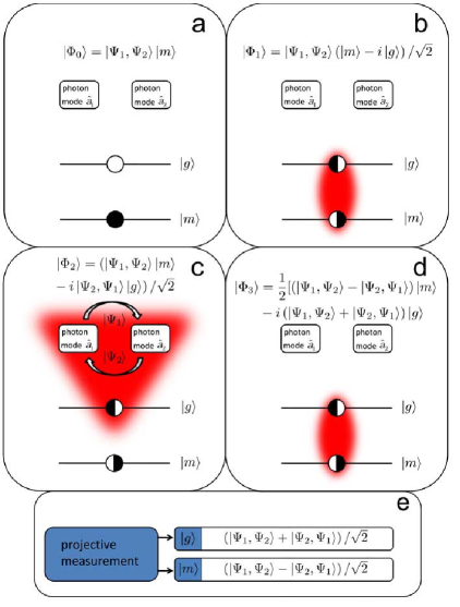
Figure 1: (color online). Conversion of the separable state into the two-mode symmetrical entangled state. a) Initial state of the system. b) Preparation of the ancilla system in the superposition state due to $\sigma^{x}$ rotation. c) Creation of the superposition of the two events - field’s state swapped and does not swapped. d) Deentanglement from the ancilla system degree of freedom due to $\sigma^{x}$ rotation. e) Projective measurement in the ancilla system subspace collapse the photon wave function into the one of the two entangled states.

The above superposition of $\left|m\right\rangle$ and $\left|g\right\rangle$ works as a logic control on the swapping between two input photonic modes: the swapping between the photon modes is activated in the $\left|g\right\rangle$ subspace and does not happen in the $\left|m\right\rangle$ subspace. Such conditional swapping can be realized by the BS transformation

$$\left(\begin{array}[c]{c}\hat{a}_{1}(t)\\ \hat{a}_{2}(t)\end{array}\right)=\left(\begin{array}[c]{cc}\cos\chi_{0}t&-ie^{i\phi}\sin\chi_{0}t\\ -ie^{-i\phi}\sin\chi_{0}t&\cos\chi_{0}t\end{array}\right)\left(\begin{array}[c]{c}\hat{a}_{1}(0)\\ \hat{a}_{2}(0)\end{array}\right)$$ (2)

for the time $t_{s}=\pi/(2\chi_{0})$, where $\hat{a}_{i}$ is the annihilation operator for the $i$-th mode and $\chi_{0}$ is the effective BS coupling constant. The BS transformation can be implemented via the dispersive parametric three-wave mixing (TWM) Serra ; lin-08 or four-wave mixing (FWM) Yavuz ; SharypovFWMSuperconductors process. The use of the dispersive type of the interaction allows to avoid the decoherence of the generated state due to incoherent scattering as during the BS interaction the ancilla system is always preserved in its ground state and only the photon states are changed. The conditional swapping results in the state

$$\left|\Phi_{2}\right\rangle=\left(\left|\Psi_{1},\Psi_{2}\right\rangle\left|m\right\rangle-i\left|\Psi_{2},\Psi_{1}\right\rangle\left|g\right\rangle\right)/\sqrt{2}.$$ (3)

Then, again we perform a $\sigma^{x}$ rotation between $\left|m\right\rangle$ and $\left|g\right\rangle$ to have them transformed as $\left|m\left(g\right)\right\rangle\rightarrow\left|m\left(g\right)\right\rangle-i\left|g\left(m\right)\right\rangle$, leading to the following state

$$\left|\Phi_{3}\right\rangle =\frac{1}{2}[\left(\left|\Psi_{1},\Psi_{2}\right\rangle-\left|\Psi_{2},\Psi_{1}\right\rangle\right)\left|m\right\rangle$$

$$-i\left(\left|\Psi_{1},\Psi_{2}\right\rangle+\left|\Psi_{2},\Psi_{1}\right\rangle\right)\left|g\right\rangle.$$ (4)

Finally, by measuring $\left|m\right\rangle$ and $\left|g\right\rangle$ (see the method in the following example), we make the photonic sector of the total state collapse to the target symmetric entangled states $\left|\Psi_{1},\Psi_{2}\right\rangle\pm\left|\Psi_{2},\Psi_{1}\right\rangle$. For clarity the complete procedure of the above is summarized in Fig. 1.

A candidate for the ancilla system should satisfy two requirements. First, the quantum system should have two long-lived and well separated states between which a $\sigma^{x}$ rotation can be performed. The second requirement is specified by the swapping stage—the system should have an appropriate energy level structure for the formation of the TWM or FWM interaction loop where two of the transitions have to be strongly coupled to the input fields. These conditions can be satisfied by certain trapped natural atoms or ions, single color centers, quantum dots or superconducting qubits based on the Josephson junctions, which have multi-level structures and can also be strongly coupled to the suitable field modes.

Different from the idea of inducing the conditional interaction of matter wave (ion or atom) state superposition with one optical mode catTheory for creating the cat states cat1 ; cat2 ; cat3 ; gerry , our setup allows to realize a conditional coupling directly between two photonic modes for their swapping. This is necessary for constructing a SECS $|\alpha,\beta\rangle\pm|\beta,\alpha\rangle$ with $\alpha\gg\beta$ (for making a cat state of large size) or a N00N state. Our method aims to generate all such states in a unified way.

III Example of realization

Here we provide an example to implement the protocol with the single ion of calcium $Ca^{+}$ trapped in ion trap and embedded in optical resonator as the ancilla system. The energy level structure of the calcium ion $Ca^{+}$ is illustrated in Fig. 2(a). Trapped ions are well studied systems for quantum information processing ion . The construction of multi-partite entangled states of trapped ions themselves has been proposed in lamata . Our proposed setup for entangling cavity fields via a trapped ion is similar to that of the recent experiments reported in blatt ; Stute2012 .

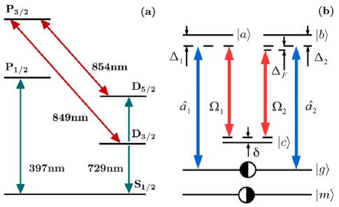
Figure 2: (color online). (a) $Ca^{+}$ energy level scheme. (b) Level scheme for realizing the conditional BS coupling between two photonic modes $\widehat{a}_{1}$ and $\widehat{a}_{2}$ (blue arrows). The red arrows represent the classical coupling fields. The white and black circles on levels $\left|g\right\rangle$ and $\left|m\right\rangle$ indicate that they are in a superposition and only one of them is involved into the parametric loop. The energy levels of this general scheme correspond to those of $Ca^{+}$ for our example as follows: $\left|m\right\rangle\rightarrow$ $4S_{1/2}\left(F=4,~{}m_{J}=0\right)$; $\left|g\right\rangle\rightarrow$ $3D_{5/2}\left(F=6,~{}m_{J}=0\right)$; $\left|a\right\rangle\rightarrow$ $4P_{3/2}\left(F=5,~{}m_{J}=1\right)$; $\left|b\right\rangle\rightarrow$ $4P_{3/2}\left(F=5,~{}m_{J}=-1\right)$ and $\left|c\right\rangle\rightarrow$ $3D_{3/2}\left(F=5,~{}m_{J}=0\right)$.

The two ground states $\left|m\right\rangle$ and $\left|g\right\rangle$ of the ancilla ion we use are $4S_{1/2}\left(F=4,~{}m_{J}=0\right)$ and $3D_{5/2}\left(F=6,~{}m_{J}=0\right)$, respectively. These particular levels are chosen as the ground states for two reasons. First, both of the states are long-lived (up to the order of $1$ s). Second, due to the selection rule and large energy difference between them, one of the ground states is excluded from our parametric FWM loop to swap two photonic modes so that the conditional BS coupling can be realized.

The photonic modes we will swap are prepared as the steady-state fields of the cavity. The process building up the steady cavity field can be described by the Hamiltonian ($\hbar\equiv 1$)

$$H_{c} =\sum_{j=1}^{2}\big{\{}iE_{j}(\hat{a}_{j}^{\dagger}e^{-i\Delta_{0j}t}-\hat{a}_{j}e^{i\Delta_{0j}t})$$

$$+i\sqrt{\kappa}\big{(}\hat{a}_{j}^{\dagger}\hat{\xi}_{c}(t)-\hat{a}_{j}\hat{\xi}_{c}^{\dagger}(t)\big{)}\big{\}}$$ (5)

in the interaction picture with respect to the cavity Hamiltonian $\sum_{j}\omega_{cj}\hat{a}_{j}^{\dagger}\hat{a}_{j}$. The first term in the above describes the continuous wave (CW) drives of the frequency $\omega_{0j}$, and with the intensity $E_{j}$ and the detuning $\Delta_{0j}=\omega_{cj}-\omega_{0j}$ from the cavity frequency $\omega_{cj}$. The second term about the coupling between the cavity modes and the cavity noise operator $\hat{\xi}_{c}$ gives rise to the damping of the cavity at the rate $\kappa$ noise ; h-12-2 . The steady cavity fields in the coherent state with $|\langle\hat{a}_{j}\rangle|=E_{j}/(0.5\kappa+i\Delta_{0j})$ will be created by driving the cavity for a while. The cavity fields in Fock state can be established by the technique in LawEberly . The two prepared intra-cavity modes in the state $\left|\Psi_{1}\right\rangle_{\sigma^{+}}$ and $\left|\Psi_{2}\right\rangle_{\sigma^{-}}$ of the different polarization will be coupled to the transition $3D_{5/2}\left(F=6\right)\leftrightarrow P_{3/2}\left(F=5\right)$ at $854$ nm of the trapped ion.

In case when the intra-cavity modes are in the coherent states the SECSs will be generated and for the Fock and vacuum inputs the N00N states will be obtained as the result of the conditional swapping. As follows from the interaction configuration presented in Fig.2(b) only the ground state $\left|g\right\rangle$ ($3D_{5/2}\left(F=6,~{}m_{J}=0\right)$) becomes coupled to the optical modes but there is no coupling to the optical modes for the state $\left|m\right\rangle$ ($4S_{1/2}\left(F=4,~{}m_{J}=0\right)$). In order to perform a $\sigma^{x}$ rotation between $\left|m\right\rangle$ and $\left|g\right\rangle$ and bring the ion into the superposition state in Eq. (1), a resonant $\pi/2$ laser pulse at $729$ nm with $\pi$ - polarization is applied to the quadrupole transition $4S_{1/2}\leftrightarrow 3D_{5/2}$. During the swapping stage there are also two classical pumping pulses with the orthogonal circular polarizations applied to the transitions $3D_{3/2}\left(F=5,m_{J}=0\right)\leftrightarrow 4P_{3/2}\left(F=5,m_{J}=\pm 1\right)$ at $849$ nm, while the cavity modes $\sigma^{+}$ and $\sigma^{-}$ are coupled to the transitions $3D_{5/2}\left(F=6,m_{J}=0\right)\leftrightarrow 4P_{3/2}\left(F=5,m_{J}=\pm 1\right)$ in the parametric FWM loop.

To realize the parametric BS coupling, all real transitions in the loop should be suppressed and ideally the ion should stay in its ground state during the swapping process. Therefore all fields should be highly detuned from the resonance and satisfy certain conditions (see the discussion below). By controlling the duration of the classical pulses we can control the precise parametric interaction time for obtaining the state in (3). After another $\pi/2$ laser pulse at $729$ nm with $\pi$ - polarization there will be the state in (4). The detection of the ground states for the final projection onto the target states is implemented by exciting the transition $4S_{1/2}\rightarrow 4P_{1/2}$ at $397$ nm; see the similar technique in detect ; detect1 . The presence of the fluorescence collapses the ion wave function onto $\left|m\right\rangle$ and the absence of the fluorescence indicates the state $\left|g\right\rangle$.

IV mechanism for induced Beam-splitter coupling

The dispersive FWM process for realizing the conditional swapping in our protocol can be implemented in any system with the level scheme in Fig. 2(b). The Hamiltonian for the process shown in Fig. 2(b) takes the form ($\hbar\equiv 1$)

$$H =-\Delta_{1}\sigma_{aa}-\Delta_{2}\sigma_{bb}-\delta\sigma_{cc}+g_{1}\widehat{a}_{1}^{\dagger}\sigma_{ga}$$

$$+g_{2}\widehat{a}_{2}^{\dagger}\sigma_{gb}+\Omega_{1}\sigma_{ca}+\Omega_{2}e^{i\Delta_{F}t}\sigma_{cb}+h.c.$$ (6)

in a rotated frame. Here $\sigma_{ij}=\left|i\right\rangle\left\langle j\right|$ is the atomic spin flip operator; $g_{1\left(2\right)}$ is the coupling constant; $\Delta_{1(2)}=\omega_{a1(2)}-\omega_{ga(b)}$ is the one-photon detuning, $\delta=\omega_{a1}-\omega_{1}-\omega_{cg}$ is the two-photon detuning, and $\Delta_{F}=\omega_{a1}-\omega_{1}-\omega_{a2}+\omega_{2}$ is the four-photon detuning, with $\omega_{1(2)}$ being the frequency of the classical pumping pulse with the Rabi frequency $\Omega_{1(2)}$, $\omega_{a1(a2)}$ being the frequency of the input pulse. The modes $\hat{a}_{i}$ are the steady field intra-cavity modes for the example described in the last section. Given the possibility to prepare the many-body superposition $(|m_{1},\cdots,m_{n}\rangle-i|g_{1},\cdots,g_{n}\rangle)/\sqrt{2}$ of an ensemble of the atoms with a similar level scheme to Fig.2(b), the dispersive FWM process can also be performed in the ensemble. Then $\hat{a}_{i}$ are just the representative modes of the narrow band input pulses.

The Hamiltonian (6) only presents the coherent part of the interaction process without dissipations. In Sec. VI we will give the detailed discussion on the decoherence effects arising due to the decay of the energy levels of the ancilla system and the loss of the cavity.

For the process in Fig.2(b) the Schrödinger equation for each energy level component of the state $|\Psi(t)\rangle$ reads:

$$i\frac{d}{dt}\left\langle g|\Psi\left(t\right)\right\rangle=g_{1}\widehat{a}_{1}^{\dagger}\left\langle a|\Psi\left(t\right)\right\rangle+g_{2}\widehat{a}_{2}^{\dagger}\left\langle b|\Psi\left(t\right)\right\rangle$$ (7a)

$$i\frac{d}{dt}\left\langle b|\Psi\left(t\right)\right\rangle =-\Delta_{2}\left\langle b|\Psi\left(t\right)\right\rangle$$

$$+ \Omega_{2}e^{-i\Delta_{F}t}\left\langle c|\Psi\left(t\right)\right\rangle+g_{2}\widehat{a}_{2}\left\langle g|\Psi\left(t\right)\right\rangle$$ (7b)

$$i\frac{d}{dt}\left\langle a|\Psi\left(t\right)\right\rangle =-\Delta_{1}\left\langle a|\Psi\left(t\right)\right\rangle$$

$$+\Omega_{1}\left\langle c|\Psi\left(t\right)\right\rangle+g_{1}\widehat{a}_{1}\left\langle g|\Psi\left(t\right)\right\rangle$$ (7c)

$$i\frac{d}{dt}\left\langle c|\Psi\left(t\right)\right\rangle =-\delta\left\langle c|\Psi\left(t\right)\right\rangle+\Omega_{1}\left\langle a|\Psi\left(t\right)\right\rangle$$

$$+\Omega_{2}e^{i\Delta_{F}t}\left\langle b|\Psi\left(t\right)\right\rangle.$$ (7d)

The effective BS Hamiltonian for the similar dispersive FWM schemes can be derived by the time-independent perturbation method SharypovFWMSuperconductors . Here we apply the more general method of the adiabatic elimination GardinerThesis to show the realization of the effective BS coupling. It is important to mention that the one- and two-photon detunings should be high enough to prevent any real transition of the system from its ground state. It is therefore possible to see the effective dynamics of the photonic modes while the system is staying in the ground state $$|g\rangle$$.

First, assuming that initially the system is prepared in its ground state $\left|g\right\rangle$, i.e. $\left\langle b|\Psi\left(t_{0}\right)\right\rangle=\left\langle a|\Psi\left(t_{0}\right)\right\rangle=\left\langle c|\Psi\left(t_{0}\right)\right\rangle=0$, we eliminate the transitions from the state $\left|g\right\rangle$ to $\left|a\right\rangle$ and $\left|b\right\rangle$. Under this assumption we integrate Eqs. (7a) - (7c) and then substitute the formal solution of $\left\langle g|\Psi\left(\tau\right)\right\rangle$ into those of $\left\langle b|\Psi\left(t\right)\right\rangle$ and $\left\langle a|\Psi\left(t\right)\right\rangle$ to obtain the relations

$$\left\langle b|\Psi\left(t\right)\right\rangle=\frac{\Omega_{2}e^{-i\Delta_{F}t}}{\Delta_{2}}\left\langle c|\Psi\left(t\right)\right\rangle+\frac{g_{2}\widehat{a}_{2}}{\Delta_{2}}\left\langle g|\Psi\left(t\right)\right\rangle$$ (8a)

$$\left\langle a|\Psi\left(t\right)\right\rangle=\frac{\Omega_{1}}{\Delta_{1}}\left\langle c|\Psi\left(t\right)\right\rangle+\frac{g_{1}\widehat{a}_{1}}{\Delta_{1}}\left\langle g|\Psi\left(t\right)\right\rangle,$$ (8b)

where we are concerned with the regime of $$\left|g_{i}\sqrt{n_{i}}/\Delta_{i}\right|\ll 1 n_{i} i$$ and keep only the first order of this small term, and is the average photon number of the -th input mode.

Next, in order to obtain the decoupled dynamics of the effective two-level system of $\left|g\right\rangle$ and $\left|c\right\rangle$, we substitute Eqs.(8a) and (8b) into Eqs. (7a) and (7d) and obtain

$$\frac{d}{dt}e^{i\alpha_{g}t}\left\langle g|\Psi\left(t\right)\right\rangle=-ie^{i\alpha_{g}t}\beta^{\dagger}\left(t\right)\left\langle c|\Psi\left(t\right)\right\rangle$$ (9a)

$$\frac{d}{dt}e^{i\alpha_{c}t}\left\langle c|\Psi\left(t\right)\right\rangle=-ie^{i\alpha_{c}t}\beta\left(t\right)\left\langle g|\Psi\left(t\right)\right\rangle,$$ (9b)

where we have introduced the functions $$\alpha_{c}=-\delta+\Omega_{1}^{2}/\Delta_{1}+\Omega_{2}^{2}/\Delta_{2} \alpha_{g}=g_{1}^{2}\widehat{a}_{1}^{\dagger}\widehat{a}_{1}/\Delta_{1}+g_{2}^{2}\widehat{a}_{2}^{\dagger}\widehat{a}_{2}/\Delta_{2} \beta=\Omega_{1}g_{1}\widehat{a}_{1}/\Delta_{1}+\Omega_{2}g_{2}\widehat{a}_{2}e^{i\Delta_{F}t}/\Delta_{2} \beta$$, , and . In the dynamics of this effective two-level system the parameter plays the role of the effective coupling constant and the parameter

$$\Delta_{eff}=\alpha_{g}-\alpha_{c}\approx\delta-\Omega_{1}^{2}/\Delta_{1}-\Omega_{2}^{2}/\Delta_{2}$$ (10)

corresponds to the effective detuning. We have considered the regime satisfying $\left|g_{i}^{2}n_{i}/\Delta_{i}\right|\ll\left|\delta-\Omega_{1}^{2}/\Delta_{1}-\Omega_{2}^{2}/\Delta_{2}\right|$ in (10). The dynamics of the states $\left|g\right\rangle$ and $\left|c\right\rangle$ will be decoupled further. Integrating Eq.(9b) we get the relation

$$\left\langle c|\Psi\left(t\right)\right\rangle=\frac{1}{\Delta_{eff}}\left[\frac{\Omega_{1}g_{1}\widehat{a}_{1}}{\Delta_{1}}+\frac{\Omega_{2}g_{2}\widehat{a}_{2}}{\Delta_{2}}e^{i\Delta_{F}t}\right]\left\langle g|\Psi\left(t\right)\right\rangle,$$ (11)

where we keep only the first order of the parameter $\left|g_{i}\sqrt{n_{i}}\Omega_{i}/\left(\Delta_{i}\Delta_{eff}\right)\right|\ll 1$.

Finally, substituting Eq. (11) into (9a), we obtain the decoupled evolution of the state $\left|g\right\rangle$

$$i\frac{d}{dt}\left\langle g|\Psi\left(t\right)\right\rangle=H_{eff}\left\langle g|\Psi\left(t\right)\right\rangle,$$ (12)

where

$$H_{eff}(t)=\eta_{1}\widehat{a}_{1}^{\dagger}\widehat{a}_{1}+\eta_{2}\widehat{a}_{2}^{\dagger}\widehat{a}_{2}+\chi_{0}\left(\widehat{a}_{1}^{{\dagger}}\widehat{a}_{2}e^{i\Delta_{F}t}+h.c.\right)$$ (13)

is the effective Hamiltonian for the photonic modes, with $\eta_{i}=\frac{g_{i}^{2}}{\Delta_{i}}+\frac{g_{i}^{2}\Omega_{i}^{2}}{\Delta_{i}^{2}\Delta_{eff}}$, $\chi_{0}=\frac{\Omega_{1}\Omega_{2}g_{1}g_{2}}{\Delta_{1}\Delta_{2}\Delta_{eff}}$.

The conditions $\left|g_{i}\sqrt{n_{i}}/\Delta_{i}\right|\ll 1$, $\left|g_{i}\sqrt{n_{i}}\Omega_{i}/\left(\Delta_{i}\Delta_{eff}\right)\right|\ll 1$ leading to the above effective dynamics prevent the one- and two-photon transitions out of a ground level and can be realized by adjusting the system parameters. For our example using $Ca^{+}$ with $g_{1(2)}\sim 10$ MHz, it is possible to set the Rabi frequencies $\Omega_{1(2)}\sim 1$ GHz, the one-photon detunings $\Delta_{1(2)}\sim 1$ GHz, and the two-photon detuning $\delta\sim 1$ GHz, given the average photon numbers up to $n_{i}=100$. The symbol “$\sim$” means the order of the values here. The sizes $\sqrt{n_{i}}$ of the states to be entangled can be made larger simply by increasing the detunings.

V performance of Swapping operation

The unitary evolution operator of the time-dependent effective Hamiltonian $H_{eff}$ in (13) can be decomposed as

$$\mbox{T}\exp\left\{-i\int_{0}^{t}d\tau H_{eff}(\tau)\right\}=\exp\left\{-i\eta_{1}\widehat{a}_{1}^{{\dagger}}\widehat{a}_{1}t-i\eta_{2}\widehat{a}_{2}^{{\dagger}}\widehat{a}_{2}t\right\}$$

$$\times\mbox{T}\exp\left\{-i\chi_{0}\int_{0}^{t}e^{-i\delta_{F}\tau}d\tau~{}\widehat{a}_{1}\widehat{a}_{2}^{{\dagger}}+h.c.\right\},$$ (14)

where T stands for a time-ordered operation and $\delta_{F}=\Delta_{F}+\eta_{1}-\eta_{2}$. The general form of such decomposition is given in h-12-2 . The first of the decomposed operators in Eq.(14) is a phase shift operation and the second is a BS operation. For example, by tuning the system parameters so that the conditions $\delta_{F}=0$ and $\Delta_{eff}=-2\Delta_{i}$ (assuming $g_{1}=g_{2}$ and $\frac{\Omega_{1}}{\Delta_{1}}=\frac{\Omega_{2}}{\Delta_{2}}=1$) are satisfied, their combined action implements an ideal swapping $\widehat{a}_{1}\leftrightarrow\widehat{a}_{2}$ after the time $t_{s}$ accumulating $|\chi_{0}t_{s}|=0.5\pi$. Given the data following Eq.(13) a pair of input states could be entangled within a few microseconds.

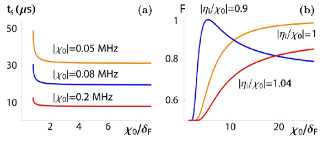
Figure 3: (color online). (a) Relation between the swapping time and the ratio $\chi_{0}/\delta_{F}$. (b) Fidelity of the generated states with the target output $|\alpha\rangle|\beta\rangle\pm|\beta\rangle|\alpha\rangle$ with $\alpha=6\sqrt{2}$ and $\beta=\sqrt{2}$, which can be converted to the cat states $|\gamma\rangle\pm|-\gamma\rangle$ of $\gamma=5$. A unit fidelity can be reached in the regime $|\eta_{i}/\chi_{0}|<1$ at a not so large ratio $\chi_{0}/\delta_{F}$.

In a general situation the swapping time $t_{s}$ is determined by the relation $2\chi_{0}\sin(0.5\delta_{F}t_{s})/\delta_{F}=0.5\pi$, implying a quickly stabilized swapping time with increasing ratio $\chi_{0}/\delta_{F}$; see Fig. 3(a). Meanwhile the output state will be $|\alpha,\beta\rangle\pm|\beta e^{i\varphi_{1}},\alpha e^{i\varphi_{2}}\rangle$, where $\varphi_{i}=\eta_{i}t_{s}-0.5\pi+0.5\delta_{F}t_{s}$, if the inputs are two coherent states $|\alpha\rangle$ and $|\beta\rangle$. The fidelity of the output state is determined by the two ratios $|\chi_{0}/\delta_{F}|$ and $|\eta_{i}/\chi_{0}|$ (given $\eta_{1}=\eta_{2}$). As it is shown in Fig. 3(b), a high-quality output state will be realized with the proper ratios that can be achieved by adjusting the system parameters.

The frequency dependent parameters in the effective Hamiltonian (13) might also decrease the BS fidelity when one considers the multi-frequency pulses. In fact, such difference is negligible to the narrow-band input pulses and can be avoided by using the interaction scheme for the BS transformation lin-08 where the effective Hamiltonian is insensitive to the frequencies of the input modes.

VI Decoherence effects

For the ancilla system applied in the parametric loop, the decoherence effect is from two sources. One is due to the broadening of the transitions, so the fields detuning $\Delta_{i}$, $\Delta_{eff}$ should be much larger than the bandwidth of the corresponding transitions $\Gamma_{gi}$ ($i=a,b$ and $c$), i.e. $\left|\Delta_{i}\right|\gg\Gamma_{ga,gb}$ and $\left|\Delta_{eff}\right|\gg\Gamma_{gc}$. The other more significant one comes from the possible population of the other energy levels than the ground state $|g\rangle$ during the swapping process. The radiative decay in the system occurs only after the excitation of the system from the ground state. As we apply a dispersive interaction, the probability for the one-photon excitation scales as $P_{a,b}=g_{1,2}^{2}n_{1,2}\Delta_{1,2}^{-2}$ (see Eqs. (8a) and (8b)), and the probability of the two-photon excitation scales as $P_{c}=|\Omega_{1}g_{1}\sqrt{n_{1}}/(\Delta_{1}\Delta_{eff})+\Omega_{2}g_{2}\sqrt{n_{2}}e^{i\Delta_{F}t}/(\Delta_{2}\Delta_{eff})|^{2}$ (see Eq. (11)). Therefore the effective decays in the system should be described by the product of the decay rate of the particular state and the probability of the electron excitation at this level. In order to have the negligible contribution from the decay processes, the swapping time should be much shorter than the effective radiative lifetime $t_{s}\ll 1/(\gamma_{i}P_{i})$. For example, if one takes the swapping time for the matched four-photon detuning giving $\delta_{F}=0$, there should be the condition $\gamma_{a,b}\ll\frac{2}{\pi}\left|\frac{\Omega_{1}\Omega_{2}}{\Delta_{eff}}\frac{\Delta_{1,2}}{\Delta_{2,1}}\frac{g_{2,1}}{g_{1,2}}\right|$ for neglecting the decay of the intermediate states $\left|a\right\rangle$ ($\left|b\right\rangle$) and the condition $\gamma_{c}\ll\frac{2}{\pi}|\sqrt{n_{1}m}+\sqrt{n_{2}e^{i\Delta_{F}t}m^{-1}}|^{-2}\left|\Delta_{eff}\right|$, where $m=\frac{\Omega_{1}g_{1}\Delta_{2}}{\Omega_{2}g_{2}\Delta_{1}}$, for neglecting the decay of the state $\left|c\right\rangle$. For the example using $Ca^{+}$ with $\gamma_{a,b}\sim 10$ MHz and $\gamma_{c}\sim 10$ Hz the above conditions can be easily established. These conditions guarantee the outputs of the swapping process to be pure states.

Another type of decoherence arises from the loss of steady cavity fields in any cavity based implementation. It modifies the unitary evolution in (14) to a non-unitary one governed by the mater equation

$$\dot{\rho}=-i[H_{eff},\rho]+\sum_{i}\kappa\big{(}\hat{a}_{i}\rho\hat{a}_{i}^{\dagger}-\frac{1}{2}(\rho\hat{a}_{i}^{\dagger}\hat{a}_{i}+\hat{a}_{i}^{\dagger}\hat{a}_{i}\rho)\big{)},$$

where $H_{eff}$ is given in (13). Given the input as a product of two coherent states $|\alpha\rangle|\beta\rangle$, for example, the solution to the master equation for a short evolution time and under the condition of reaching the unit fidelity in Fig. 3(b) can be found by following a similar procedure in h-09 as

$$\rho(t) =\frac{1}{N_{\alpha,\beta}}\big{(}|\alpha e^{-\kappa t/2},\beta e^{-\kappa t/2}\rangle\langle\alpha e^{-\kappa t/2},\beta e^{-\kappa t/2}|$$

$$+|\beta e^{-\kappa t/2},\alpha e^{-\kappa t/2}\rangle\langle\beta e^{-\kappa t/2},\alpha e^{-\kappa t/2}|$$

$$+C|\alpha e^{-\kappa t/2},\beta e^{-\kappa t/2}\rangle\langle\beta e^{-\kappa t/2},\alpha e^{-\kappa t/2}|$$

$$+C|\beta e^{-\kappa t/2},\alpha e^{-\kappa t/2}\rangle\langle\alpha e^{-\kappa t/2},\beta e^{-\kappa t/2}|,$$ (15)

where $\sqrt{N_{\alpha,\beta}}$ is the normalization factor for the SECS $|\alpha\rangle|\beta\rangle+|\beta\rangle|\alpha\rangle$, and $C=\exp\{-2|\alpha-\beta|^{2}(1-e^{-\kappa t})\}$. Such decoherence could be negligible to a cavity of high finesse. Using a cavity with the damping time $0.13$ seconds as in cat3 , for example, the fidelity (with a pure SECS) of the generated state for the example in Fig. 3(b) can be preserved over $0.98$ up to the conditional swapping time $0.1$ milliseconds.

VII conclusion

With an example, we have illustrated how to entangle two arbitrary states $|\Psi_{1}\rangle$ and $|\Psi_{2}\rangle$ to the symmetric form $\left|\Psi_{1},\Psi_{2}\right\rangle\pm\left|\Psi_{2},\Psi_{1}\right\rangle$ with an induced conditional BS type coupling that avoids the physical limitation on nonlinear couplings. In contrast to all previous schemes, the entanglement strategy is independent of the specific input states, e.g. SECSs and N00N states can be generated in the same way. The FWM process for realizing the effective BS coupling is within the current experimental technology. This approach can help to achieve the goals of entangling light fields with flexibility and creating cat states of large size.

- (1) B. C. Sanders, J. Phys. A: Math. Theor. 45, 244002 (2012).
- (2) B. C. Sanders, Phys. Rev. A 40, 2417 (1989).
- (3) A. N. Boto, et al., Phys. Rev. Lett. 85, 2733 (2000).
- (4) H. Lee, P. Kok, and J. P. Dowling, J. Mod. Opt. 49, 2325 (2002).
- (5) T. C. Ralph, Phys. Rev. A 65, 042313 (2002).
- (6) S. Glancy and H. M. Vasconcelos, J. Opt. B: Quantum Semiclassical Opt. 25, 712 (2008).
- (7) C. Monroe, et al., Science 272, 1131 (1996).
- (8) M. Brune, et al., Phys. Rev. Lett. 77, 4887 (1996).
- (9) S. Deleglise, et al., Nature (London) 455, 510 (2008).
- (10) B. Yurke and D. Stoler, Phys. Rev. Lett. 57, 13 (1986).
- (11) S. Song, C. M. Caves, and B. Yurke, Phys. Rev. A41, 5261 (1990).
- (12) M. Dakna, et al., Phys. Rev. A55, 3184 (1997).
- (13) H. Jeong, Phys. Rev. A 72, 034305 (2005).
- (14) M. S. Kim and M. Paternostro, J. Mod. Opt. 54, 155 (2007).
- (15) B. He, M. Nadeem, and J. A. Bergou, Phys. Rev. A79, 035802 (2009).
- (16) J. Gea-Banacloche, Phys. Rev. A81, 043823 (2010).
- (17) B. He and A. Scherer, Phys. Rev. A85, 033814 (2012).
- (18) B. He, et al., Phys. Rev. A83, 022312 (2011).
- (19) B. He, Q. Lin, and C. Simon, Phys. Rev. A 83, 053826 (2011).
- (20) R. M. Serra, et al., Phys. Rev. A 71, 045802 (2005).
- (21) G.-W. Lin, et al., Phys. Rev. A77, 064301 (2008).
- (22) D. D. Yavuz, Phys. Rev. A 71, 053816 (2005).
- (23) A. V. Sharypov, X. Deng, and L. Tian, Phys. Rev. B 86, 014516 (2012).
- (24) C. M. Savage, S. L. Braunstein, and D. F. Walls, Opt. Lett. 15, 628 (1990).
- (25) C. C. Gerry and P. L. Knight, Chap. 10, Introductory Quantum Optics, Cambridge University Press (2005).
- (26) H. Haeffner, C. F. Roos, and R. Blatt, Phys. Rep. 469, 155 (2008).
- (27) L. Lamata, et al., arXiv:1211.0404.
- (28) A. Stute, et al., Appl. Phys. B 107, 1147 (2012).
- (29) A. Stute et al., Nature (London) 485, 482 (2012).
- (30) C. W. Gardiner and P. Zoller, Quantum Noise (Springer-Verlag, Berlin, 2000).
- (31) B. He, Phys. Rev. A85, 063820 (2012).
- (32) C. K. Law and J. H. Eberly, Phys. Rev. Lett. 76, 1055 (1996).
- (33) F. Schmidt-Kaler, et al., Nature (London) 422, 408 (2003).
- (34) A. H. Myerson, et al., Phys. Rev. Lett. 100, 200502 (2008).
- (35) S. A. Gardiner, Quantum Measurements, Quantum Chaos, and Bose-Einstein Condensates, PhD Thesis (2000).