COLOR GLASS CONDENSATE AND GLASMA

Abstract

We review the Color Glass Condensate effective theory, that describes the gluon content of a high energy hadron or nucleus, in the saturation regime. The emphasis is put on applications to high energy heavy ion collisions. After describing initial state factorization, we discuss the Glasma phase, that precedes the formation of an equilibrated quark-gluon plasma. We end this review with a presentation of recent developments in the study of the isotropization and thermalization of the quark-gluon plasma.

PACS numbers: 12.20.-m, 11.10.Hi, 11.15.Kc, 11.80.Fv, 11.80.La, 13.85.Hd

1 Introduction

Heavy Ion Collisions at high energy are performed at the Relativistic Heavy Ion Collider (RHIC) and the Large Hadron Collider (LHC), in order to study the properties of nuclear matter under extreme conditions of density and temperature. From lattice simulations[1], it is known that above a certain critical temperature, the protons and neutrons should melt into a plasma made of their constituents, the Quark-Gluon Plasma (QGP), and the critical temperature of this deconfinement transition is expected to be reached in the collisions performed at RHIC and LHC.

Figure 1: Elementary couplings between quarks and gluons in QCD.

Quantum Chromodynamics (QCD), the theory of the microscopic interactions between the quarks and the gluons (see the figure 1), should in principle also be applicable to heavy ion collisions. However, since the strong interaction coupling constant becomes large at low momentum, it is not obvious a priori that heavy ion collisions can be studied by weak coupling techniques. This is certainly possible for the rare large-momentum processes that take place in these collisions, but quite questionable for the bulk of the particle production processes. Moreover, since the system produced in such a collision expands rapidly along the collision axis (see the figure 2), its characteristic momentum scales (e.g. its temperature if it reaches thermal equilibrium) decrease with time.

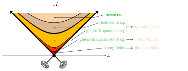
Figure 2: Successive stages of a high energy heavy ion collision, and the most widely used approaches to describe each stage.

Therefore, there will always be a time beyond which the coupling is strong and weak coupling approaches are useless. This is obviously the case near the phase transition that sees the quarks and gluons recombine in order to form hadrons. In the best of cases, we can only hope for a weak coupling treatment of the early stages of these collisions (say up to a couple of fm/c after the collision).

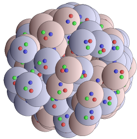
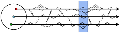
Figure 3: Parton content of a nucleon or nucleus at low energy. Left: cartoon of a nucleus at low energy and its valence quarks. Right: the thick lines represent the valence quarks, and the wavy lines are gluons. Virtual quark-antiquark pairs are not represented.

When applying QCD to the study of hadronic collisions, an essential ingredient is the quark and gluon content of the hadrons that are being collided, since the elementary degrees of freedom in QCD are partons rather than hadrons. On the surface, a nucleon is made of three valence quarks, bound by gluons. However, these quarks can also temporarily fluctuate into states that have additional gluons and quark-antiquark pairs (see the figure 3). These fluctuations are short lived, with a lifetime that is inversely proportional to their energy. The largest possible lifetime of these fluctuations is comparable to the nucleon size, and they can be arbitrarily short lived. However, in a given reaction that probes the nucleon, there is always a characteristic time scale set by the resolution power of the probe (for instance by the frequency of the virtual photon that probes the nucleon in Deep Inelastic Scattering). Only the fluctuations that are longer lived than the resolution in time of the probe can actually be seen in the process. The shorter lived fluctuations are present, but do not influence the reaction. In collisions involving a low energy nucleon, only its valence quarks and a few of these fluctuations are visible. Moreover, in a low energy nucleon, there will typically be interactions between its constituents during the collision with the probe, thus making low energy reactions very complicated.

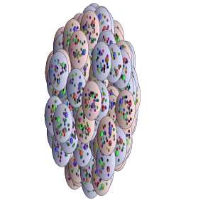
Figure 4: Parton content of a nucleon or nucleus at high energy, as seen in the laboratory frame. Left: boosted nucleus and its gluonic content. Right: fluctuations inside a boosted nucleon.

However, this picture is dramatically modified when the reaction involves a high energy nucleon, due to relativistic kinematics (see the figure 4). Firstly, the geometry of the nucleon changes due to Lorentz contraction: at very high energy, the nucleon appears essentially two-dimensional in the laboratory frame. Simultaneously, all the internal timescales of the nucleon –in particular the lifetimes of the fluctuations and the duration of the interactions among the constituents– are multiplied by the same Lorentz factor. The first consequence of this time dilation is that the partons are now unlikely to interact precisely during the time interval probed in the reaction: the constituents of a high energy nucleon appear to be free during the collision. Secondly, since the lifetimes of the fluctuations are also dilated, more fluctuations are now visible by the probe: the number of gluons seen in a reaction increases with the energy of the collision.

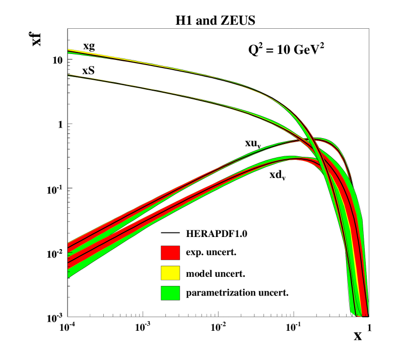
Figure 5: Parton distributions in a proton, measured in Deep Inelastic Scattering at HERA[2].

This increase with energy of the number of gluons in a nucleon has been observed experimentally in Deep Inelastic Scattering (DIS), for instance at HERA. This is shown in the figure 5 for a proton. Note that in this plot, high energy corresponds to small values of the longitudinal momentum fraction $x$ carried by the parton, $x\equiv p_{z}/\sqrt{s}$. The other important feature of the parton distributions at high energy/small $x$ is that the gluons are outnumbering all the other parton species – the valence quarks are completely negligible in this kinematical region, and the sea quarks are suppressed by one power of the coupling $\alpha_{s}$, since they are produced from the gluons by the splitting $g\to q\overline{q}$.

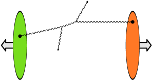
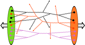
Figure 6: Left: typical process in a hadronic collision in the dilute regime. Right: typical process in the dense regime.

This increase of the gluon distribution at small $x$ leads to a major complication when applying QCD to compute processes in this regime. Indeed, the usual tools of perturbation theory are well adapted to the situation where the parton distributions are small (see the left figure 6) and where a fairly small number of graphs contribute at each order. On the contrary, when the parton distributions increase, processes involving many partons become more and more important, as illustrated in the right panel of the figure 6. The extreme situation arises when the gluon occupation number is of order $1/\alpha_{s}$: in this case, an infinite number of graphs contribute at each order. This regime of high parton densities is non-perturbative, even if the coupling constant is weak – the non-perturbative features arise from the fact that the large parton density compensates the smallness of the coupling constant. In addition to requiring the summation of an infinite set of Feynman diagrams, this situation requires some knowledge about the probability of occurrence of multigluon states in the wavefunctions of the two colliding projectiles, something which is not provided by the usual parton distributions (they give only the single parton density).

A major progress in dealing with this situation has been the realization that weak coupling methods can be used in this problem, thanks to the dynamical generation of a scale that is much larger than the non-perturbative scale $\Lambda_{{}_{QCD}}$ (the scale at which the strong interactions become really strong, and where confinement effects are crucial). This scale, known as the saturation momentum and denoted $Q_{s}$, is due to the non-linear interactions among the gluons. Roughly speaking, it is defined as the coupling constant $\alpha_{s}$ times the gluon density per unit area (because the Lorentz contraction makes the nucleus look like a flat sheet of gluons in the laboratory frame), and it is a measure of the strength of the gluon recombination processes that may occur when the gluon density becomes large[3, 4, 5]. Any process involving momenta smaller than $Q_{s}$ may be affected by gluon saturation.

Moreover, an effective theory –known as the Color Glass Condensate (CGC)– has been developed in order to organize the calculations of processes in the saturation regime. This effective theory approximates the description of the fast partons in the wavefunction of a hadron by exploiting the fact that their dynamics is slowed down by Lorentz time dilation, and provides a way to track the evolution with energy of the multigluon states that are relevant in the dense regime. This framework has been applied to a range of reactions at high energy: DIS, proton-nucleus collisions and nucleus-nucleus collisions. At leading order, these calculations correspond to a classical field description of the system. In nucleus-nucleus collisions, this classical field remains coherent for a brief amount of time after the collision, forming a state know as the Glasma. A central question in heavy ion collisions is to understand how these classical fields lose their coherence in order to form a plasma of quarks and gluons in local thermal equilibrium.

The purpose of these lectures is to expose the physics of the Color Glass Condensate and of the Glasma. The main focus will be heavy ion collisions, except for the first sections where the simpler example of DIS is used in order to introduce the concept of gluon saturation and the CGC framework. Our emphasis is to present a consistent framework to describe heavy ion collisions from the pre-collision initial state to the time at which the system may be described by hydrodynamics. The outline is the following:

• In the section 2, we discuss the evolution of the wavefunction of a color singlet dipole, and derive the BFKL and BK equations. This will provide a first glimpse at gluon saturation, and allow us to explain some interesting scaling properties for the inclusive DIS cross-section.

• In the section 3, we introduce the Color Glass Condensate effective theory, as a more general way to describe the saturation regime.

• The section 4 is devoted to a discussion of the factorization of the logarithms that appear in loop calculations in the CGC framework, for heavy ion collisions. We show how these logarithms can be absorbed into universal distributions that describe the multigluon content of the two colliding nuclei.

• In the section 5, we present the main ideas of the Glasma picture, and discuss some phenomenological consequences that follow from it.

• The section 6 discusses the final state evolution, that leads from the coherent Glasma fields to the thermalized quark gluon plasma. The main focus is on the instabilities of the classical solutions of the Yang-Mills equations, their resummation, and their possible role in the isotropization and thermalization processes.

2 Hadron wavefunction at high energy

In order to introduce the physics of gluon saturation, we consider in this section the case of Deep Inelastic Scattering. This situation is one of the simplest, since only one of the two projectiles is a hadron, the other being a lepton that interacts only electromagnetically via a photon exchange. DIS can viewed as an interaction between a photon with a negative virtuality ($q_{\mu}q^{\mu}=-Q^{2}<0$) and the hadronic target.

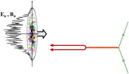
Figure 7: Cartoon of Deep Inelastic Scattering in a frame where the photon fluctuates into a dipole.

The cross-section for this process is frame independent, but in this section we will analyze it in a frame where the photon has a large longitudinal momentum, while the hadron has only a moderate momentum. In such a frame, the photon can fluctuate into a quark-antiquark pair in a color singlet state (called a color dipole), and it is this pair that interacts with the colored constituents of the target. Moreover, at high energy, this dipole sees the constituents (quarks and gluons) as frozen due to time dilation. Therefore, its interactions with these constituents can be approximated as interactions with the (static) color field that they create. Moreover, thanks to confinement, it is legitimate to assume that this target color field occupies a bounded region of space.

2.1 Eikonal approximation

We will compute the total cross-section between the dipole and the target field by using the optical theorem, that relates the total cross-section to the forward scattering amplitude. In the limit where the longitudinal momentum of the dipole is very large, this amplitude becomes very simple and is given by the eikonal approximation. Since this is an extremely important result in the study of high energy scattering, let us derive it in detail. Consider an $S$-matrix element,

$$S_{\beta\alpha}\equiv\big{<}\beta{}_{\rm out}\big{|}\alpha{}_{\rm in}\big{>}={\big{<}\beta_{\rm in}}\big{|}U(+\infty,-\infty)\big{|}{\alpha_{\rm in}\big{>}}\;,$$ (1)

for the transition between two arbitrary states made of quarks, antiquarks and gluons, $\alpha$ and $\beta$. In the second equality, $U(+\infty,-\infty)$ is the evolution operator from the initial to the final state. It can be expressed as the time ordered exponential of the interaction part of the Lagrangian,

$$U(+\infty,-\infty)=T\,\exp\Big{[}i\int d^{4}x\;{\cal L}_{\rm int}(\phi_{\rm in}(x))\Big{]}\;,$$ (2)

where $\phi_{\rm in}$ denotes generically the fields in the interaction picture. In our problem, ${\cal L}_{\rm int}$ contains both the self-interactions of the fields, and their interaction with the target color field. We want to compute the high energy limit of this scattering amplitude,

$$S_{\beta\alpha}^{(\infty)}\equiv\lim_{\omega\to+\infty}{\big{<}\beta_{\rm in}}\big{|}{e^{-i\omega K^{3}}}U(+\infty,-\infty)\underbrace{{e^{+i\omega K^{3}}}\big{|}{\alpha_{\rm in}\big{>}}}_{\mbox{\scriptsize boosted state}}$$ (3)

where ${K^{3}}$ is the generator of Lorentz boosts in the $+z$ direction.

Before doing any calculation, a simple argument can help understand what happens in this limit. Quite generally, scattering amplitudes are proportional to the duration of the overlap between the wavefunctions of the two colliding objects. In the present case, it should scale as the time spent by the incoming state in region occupied by the target field. This time is inversely proportional to the energy of the incoming state, and goes to zero in the limit $\omega\to+\infty$. If the interaction between the projectile and the target field was via a scalar exchange, then the conclusion would be that the scattering amplitude vanishes in the high energy limit (in other words, $S$-matrix elements would go to unity). However, interactions with a color field are via a vector exchange, i.e. the target field couples to a four-vector that represents the color current carried by the projectile, by a term of the form $-ig{\cal A}_{\mu}J^{\mu}$. At high energy, the longitudinal component of this four-vector increases proportionally to the energy, and compensates the small time spent in the interaction zone. Thus, for states that interact via a vector exchange, we expect that scattering amplitudes have a finite high energy limit (nor zero, nor infinite).

This calculation is best done using light-cone coordinates. For any four-vector $a^{\mu}$, one defines

$${a^{+}}\equiv\frac{a^{0}+a^{3}}{\sqrt{2}}\quad,\quad{a^{-}}\equiv\frac{a^{0}-a^{3}}{\sqrt{2}}\;.$$ (4)

The following formulas are often useful,

$$x\cdot y=x^{+}y^{-}+x^{-}y^{+}-{\boldsymbol{x}}_{\perp}\cdot{\boldsymbol{y}}_{\perp}$$

$$d^{4}x=dx^{+}dx^{-}d^{2}{\boldsymbol{x}}_{\perp}$$

$$\square=2\partial^{+}\partial^{-}-{\boldsymbol{\nabla}}_{\perp}^{2}\qquad\mbox{with}\quad\partial^{+}\equiv\frac{\partial}{\partial x^{-}}\;,\;\partial^{-}\equiv\frac{\partial}{\partial x^{+}}\;.$$ (5)

For a highly boosted projectile in the $+z$ direction, $x^{+}$ plays the role of the time, and the Hamiltonian is the $P^{-}$ component of the momentum. The generator of longitudinal boosts in light-cone coordinates is

$$K^{-}\equiv M^{-+}=-K^{3}\;.$$ (6)

In order to derive the eikonal approximation, the following identities are also very useful,

$$e^{i\omega K^{-}}\;{P^{-}}\;e^{-i\omega K^{-}} = e^{-\omega}{P^{-}}$$

$$e^{i\omega K^{-}}\;{P^{+}}\;e^{-i\omega K^{-}} = e^{+\omega}{P^{+}}$$

$$e^{i\omega K^{-}}\;{P^{j}}\;e^{-i\omega K^{-}} = {P^{j}}\;.$$ (7)

They express the fact that, under longitudinal boosts, the components $P^{\pm}$ of a four-vector are simply rescaled, while the transverse components are left unchanged.

Under longitudinal boosts, states, creation operators and field operators are transformed as follows,

$${e^{-i\omega K^{-}}}\big{|}{\boldsymbol{p}}\cdots{}_{\rm in}\big{>}=\big{|}({e^{\omega}}p^{+},{\boldsymbol{p}}_{\perp})\cdots{}_{\rm in}\big{>}$$

$${e^{-i\omega K^{-}}}a^{\dagger}_{\rm in}(q){e^{i\omega K^{-}}}=a^{\dagger}_{\rm in}({e^{\omega}}q^{+},{e^{-\omega}}q^{-},{\boldsymbol{q}}_{\perp})$$

$$\vphantom{\int}{e^{i\omega K^{-}}}\phi_{\rm in}(x){e^{-i\omega K^{-}}}=\phi_{\rm in}({e^{-\omega}}x^{+},{e^{\omega}}x^{-},{\boldsymbol{x}}_{\perp})\;.$$ (8)

Note that the last equation is valid only for a scalar field, or for the transverse components of a vector field. In addition, the $\pm$ components of a vector field receive an overall rescaling by a factor $e^{\pm\omega}$. Moreover, since a longitudinal boost does not alter the time ordering, we can also write

$${e^{i\omega K^{-}}}U(+\infty,-\infty){e^{-i\omega K^{-}}}=T\exp i\int d^{4}x\;{\cal L}_{\rm int}({e^{i\omega K^{-}}}\phi_{\rm in}(x){e^{-i\omega K^{-}}})\;.$$ (9)

Likewise, the components of the vector current that couples to the target field transform as

$${e^{i\omega K^{-}}}J^{i}(x){e^{-i\omega K^{-}}}=J^{i}({e^{-\omega}}x^{+},{e^{\omega}}x^{-},{\boldsymbol{x}}_{\perp})$$

$${e^{i\omega K^{-}}}J^{-}(x){e^{-i\omega K^{-}}}={e^{-\omega}}\,J^{-}({e^{-\omega}}x^{+},{e^{\omega}}x^{-},{\boldsymbol{x}}_{\perp})$$

$${e^{i\omega K^{-}}}J^{+}(x){e^{-i\omega K^{-}}}={e^{\omega}}\,J^{+}({e^{-\omega}}x^{+},{e^{\omega}}x^{-},{\boldsymbol{x}}_{\perp})\;.$$ (10)

Naturally, the target field ${\cal A}_{\mu}$ does not change when we boost the projectile. For simplicity, let us assume that ${\cal A}_{\mu}$ is confined in the region $-L\leq x^{+}\leq+L$. We can split the evolution operator into three factors,

$$U(+\infty,-\infty)=U(+\infty,+L)U(+L,-L)U(-L,-\infty)\;.$$ (11)

The factors $U(+\infty,+L)$ and $U(-L,-\infty)$ do not contain the external potential. For these two factors, the change of variables $e^{-\omega}x^{+}\to x^{+}$, $e^{\omega}x^{-}\to x^{-}$ leads to

$$\lim_{\omega\to+\infty}{e^{i\omega K^{-}}}U(+\infty,+L){e^{-i\omega K^{-}}} = U_{0}(+\infty,0)$$

$$\lim_{\omega\to+\infty}{e^{i\omega K^{-}}}U(-L,-\infty){e^{-i\omega K^{-}}} = U_{0}(0,-\infty)\;,$$ (12)

where $U_{0}$ is the same as $U$, but with the self-interactions only (since these two factors correspond to the evolution of the projectile while outside of the target field). For the factor $U(+L,-L)$, the change $e^{\omega}x^{-}\to x^{-}$ gives

$$\lim_{\omega\to+\infty}{e^{i\omega K^{-}}}U(+L,-L){e^{-i\omega K^{-}}}=\exp\Big{[}i{g}\int d^{2}{\boldsymbol{x}}_{\perp}\;{\chi({\boldsymbol{x}}_{\perp})}\,{\rho({\boldsymbol{x}}_{\perp})}\Big{]}\;,$$ (13)

$$\mbox{with}\qquad\left\{\begin{aligned} &{\chi({\boldsymbol{x}}_{\perp})}\equiv\int dx^{+}\;{{\cal A}^{-}(x^{+},0,{\boldsymbol{x}}_{\perp})}\\ &{\rho({\boldsymbol{x}}_{\perp})}\equiv\int dx^{-}\;{J^{+}(0,x^{-},{\boldsymbol{x}}_{\perp})}\;.\end{aligned}\right.$$ (14)

Thus, the high-energy limit of the scattering amplitude is

$$S_{\beta\alpha}^{(\infty)}={\big{<}\beta_{\rm in}\big{|}}U_{0}(+\infty,0)\;\exp\Big{[}i{g}\int d^{2}{\boldsymbol{x}}_{\perp}\;{\chi({\boldsymbol{x}}_{\perp})}{\rho({\boldsymbol{x}}_{\perp})}\Big{]}U_{0}(0,-\infty){\big{|}\alpha_{\rm in}\big{>}}\;.$$ (15)

A few remarks are in order at this point

• Only the ${\cal A}^{-}$ component of the vector potential matters.

• The self-interactions and the interactions with the external potential are factorized into three separate factors – this is a generic property of high energy scattering.

• This is an exact result in the limit $\omega\to+\infty$.

Eq. (15) is an operator formula that still contains the self-interactions of the fields to all orders. In order to evaluate it, one must insert the identity operator written as a sum over a complete set of states on each side of the exponential,

$$S_{\beta\alpha}^{(\infty)}=\smash{\sum_{{\gamma},{\delta}}}{\big{<}\beta_{\rm in}\big{|}}U_{0}(+\infty,0){\big{|}\gamma_{\rm in}\big{>}}\vphantom{\Big{[}}$$

$$\qquad\quad\times{\big{<}\gamma_{\rm in}\big{|}}\exp\Big{[}i{g}{\int\limits_{{\boldsymbol{x}}_{\perp}}}{\chi({\boldsymbol{x}}_{\perp})}{\rho({\boldsymbol{x}}_{\perp})}\Big{]}{\big{|}\delta_{\rm in}\big{>}\big{<}\delta_{\rm in}\big{|}}U(0,-\infty){\big{|}\alpha_{\rm in}\big{>}}\;.$$ (16)

The factor

$$\sum_{\delta}{\big{|}\delta_{\rm in}\big{>}\big{<}\delta_{\rm in}\big{|}}U(0,-\infty){\big{|}\alpha_{\rm in}\big{>}}$$ (17)

is the Fock expansion of the initial state: it accounts for the fact that the state $\alpha$ prepared at $x^{+}=-\infty$ may have fluctuated into another state $\delta$ before it interacts with the external potential. The matrix elements of $U_{0}$ that appear in this expansion can be calculated perturbatively to any desired order. There is a similar factor for the final state evolution.

The interactions with the target field are contained in the central factor, ${\big{<}\gamma_{\rm in}\big{|}}\exp...{\big{|}\delta_{\rm in}\big{>}}$. In order to rewrite it into a more intuitive form, let us first rewrite the operator $\rho$ as

$${\rho^{a}({\boldsymbol{x}}_{\perp})}={t^{a}_{ij}}\smash{\int\frac{dp^{+}}{4\pi p^{+}}\frac{d^{2}{\boldsymbol{p}}_{\perp}}{(2\pi)^{2}}\frac{d^{2}{\boldsymbol{q}}_{\perp}}{(2\pi)^{2}}}\Big{\{}{b^{\dagger}_{\rm in}(p^{+},{\boldsymbol{p}}_{\perp};i)b_{\rm in}(p^{+},{\boldsymbol{q}}_{\perp};j)}e^{i({\boldsymbol{p}}_{\perp}-{\boldsymbol{q}}_{\perp})\cdot{\boldsymbol{x}}_{\perp}}$$

$$\qquad\qquad\qquad\qquad\qquad\qquad-{d^{\dagger}_{\rm in}(p^{+},{\boldsymbol{p}}_{\perp};i)d_{\rm in}(p^{+},{\boldsymbol{q}}_{\perp};j)}e^{-i({\boldsymbol{p}}_{\perp}-{\boldsymbol{q}}_{\perp})\cdot{\boldsymbol{x}}_{\perp}}\Big{\}}\;,$$ (18)

where the $t^{a}_{ij}$ are the generators of the fundamental representation of the $SU(N)$ algebra and the $b,d,b^{\dagger},d^{\dagger}$ the annihilation and creation operators for quarks and antiquarks. $\rho^{a}$ also receives a contribution from gluons, not written here, obtained with the generators in the adjoint representation and the annihilation and creation operators for gluons instead. This formula captures the essence of eikonal scattering:

• Each annihilation operator has a matching creation operator – therefore, the number of partons in the state does not change during the scattering, nor their flavor.

• The $p^{+}$ component of the momenta are not affected by the scattering.

• Only the colors and transverse momenta of the partons can change during the scattering.

Scattering amplitudes in the eikonal limit take a very simple form if one trades transverse momentum for a transverse position, by doing a Fourier transform. For each intermediate state ${\big{<}\delta_{\rm in}\big{|}}\equiv{\big{<}\{k^{+}_{i},{\boldsymbol{k}}_{i\perp}\}\big{|}}$, define the corresponding light-cone wave function by :

$${\Psi_{\delta\alpha}(\{k^{+}_{i},{\boldsymbol{x}}_{i\perp}\})}\equiv\prod_{i\in\delta}\int\frac{d^{2}{\boldsymbol{k}}_{i\perp}}{(2\pi)^{2}}e^{-i{\boldsymbol{k}}_{i\perp}\cdot{\boldsymbol{x}}_{i\perp}}{\big{<}\delta_{\rm in}\big{|}}U(0,-\infty){\big{|}\alpha_{\rm in}\big{>}}\;,$$ (19)

where the index $i$ runs over all the partons of the state $\delta$. Then, each charged particle going through the external field acquires a phase proportional to its charge (antiparticles get an opposite phase),

$${\Psi_{\delta\alpha}(\{k^{+}_{i},{\boldsymbol{x}}_{i\perp}\})}\;\longrightarrow\;{\Psi_{\delta\alpha}(\{k^{+}_{i},{\boldsymbol{x}}_{i\perp}\})}\prod_{i}{U_{i}({\boldsymbol{x}}_{\perp})}$$

$${U_{i}({\boldsymbol{x}}_{\perp})}\equiv T\exp\Big{[}ig\int dx^{+}\;{{\cal A}^{-}_{a}(x^{+},0,{\boldsymbol{x}}_{i\perp})}{t^{a}}\Big{]}\;.$$ (20)

($U$ is replaced by $U^{\dagger}$ for antiquarks, and $t^{a}$ by an adjoint generator for gluons.) The factors $U$ in this formula are called Wilson lines.

2.2 Dipole scattering at Leading and Next to Leading Order

Let us now assume that the initial and final states ${\alpha}$ and ${\beta}$ both contain a virtual photon, as would be the case in DIS at leading order. The simplest Fock state that contributes to its wave function is a $q\overline{q}$ pair in a color singlet state, and the bare scattering amplitude can be written as

$$\propto {\Psi^{(0)*}_{ij}({\boldsymbol{x}}_{\perp},{\boldsymbol{y}}_{\perp})}{\Psi^{(0)}_{kl}({\boldsymbol{x}}_{\perp},{\boldsymbol{y}}_{\perp})}{U_{ik}({\boldsymbol{x}}_{\perp})U^{\dagger}_{lj}({\boldsymbol{y}}_{\perp})}$$ (21)

$$\propto {\left|\Psi^{(0)}({\boldsymbol{x}}_{\perp},{\boldsymbol{y}}_{\perp})\right|^{2}}{\rm tr}\left[{U({\boldsymbol{x}}_{\perp})U^{\dagger}({\boldsymbol{y}}_{\perp})}\right]\;.$$

The color trace arises because the wavefunction of the photon is diagonal in color, $\Psi_{ij}^{(0)}\sim\delta_{ij}$. In the diagram in the left hand side, the gray band represents the Lorentz contracted target field.

It turns out that one-loop corrections due to the emission of a gluon inside the dipole are enhanced by logarithms of the dipole longitudinal momentum $p^{+}$, leading to possibly large corrections proportional to $\alpha_{s}\log(p^{+})$. In order to compute the dipole amplitude at next to leading order, we need to evaluate the following graphs

We will call real the terms where the gluon traverses the target field, and virtual those where the gluon is a correction inside the wavefunction of the incoming or outgoing dipole. In the light-cone gauge $A^{+}=0$, the emission of a gluon of momentum $k$ and polarization $\lambda$ by a quark can be written as

$$\raise-8.53581pt\hbox to42.67912pt{\hfil\leavevmode\resizebox{42.67912pt}{}{\includegraphics{LCrules}}\hfil}\quad=\;2{g}t^{a}\;\frac{{\boldsymbol{\epsilon}}_{\lambda}\cdot{\boldsymbol{k}}_{\perp}}{k_{\perp}^{2}}\;,$$ (22)

where it is assumed that the gluon is soft compared to the quark and where ${\boldsymbol{\epsilon}}_{\lambda}$ is the polarization vector of the gluon. Trading transverse momentum in favor of transverse position, this vertex reads

$$\int\frac{d^{2}{\boldsymbol{k}}_{\perp}}{(2\pi)^{2}}\;e^{i{\boldsymbol{k}}_{\perp}\cdot({\boldsymbol{x}}_{\perp}-{\boldsymbol{z}}_{\perp})}\;2{g}t^{a}\;\frac{{\boldsymbol{\epsilon}}_{\lambda}\cdot{\boldsymbol{k}}_{\perp}}{k_{\perp}^{2}}=\frac{2i{g}}{2\pi}t^{a}\frac{{\boldsymbol{\epsilon}}_{\lambda}\cdot({\boldsymbol{x}}_{\perp}-{\boldsymbol{z}}_{\perp})}{({\boldsymbol{x}}_{\perp}-{\boldsymbol{z}}_{\perp})^{2}}\;.$$ (23)

The other rule we need to compute these graphs is that when connecting the gluons to form the loop, one must sum over their polarizations, leading to a factor

$$\sum_{\lambda}{\boldsymbol{\epsilon}}_{\lambda}^{i}{\boldsymbol{\epsilon}}_{\lambda}^{j}={\delta^{ij}}\;.$$ (24)

Let us start with the virtual contributions. For instance, one gets

$$= {\left|\Psi^{(0)}({\boldsymbol{x}}_{\perp},{\boldsymbol{y}}_{\perp})\right|^{2}}{\rm tr}\left[{t^{a}t^{a}}{U({\boldsymbol{x}}_{\perp})U^{\dagger}({\boldsymbol{y}}_{\perp})}\right]$$ (25)

$$\times-2{\alpha_{s}}{\int\frac{dk^{+}}{k^{+}}}\int\frac{d^{2}{\boldsymbol{z}}_{\perp}}{(2\pi)^{2}}\frac{({\boldsymbol{x}}_{\perp}-{\boldsymbol{z}}_{\perp})\cdot({\boldsymbol{x}}_{\perp}-{\boldsymbol{z}}_{\perp})}{({\boldsymbol{x}}_{\perp}-{\boldsymbol{z}}_{\perp})^{2}({\boldsymbol{x}}_{\perp}-{\boldsymbol{z}}_{\perp})^{2}}\;,$$

and

$$= {\left|\Psi^{(0)}({\boldsymbol{x}}_{\perp},{\boldsymbol{y}}_{\perp})\right|^{2}}{\rm tr}\left[{t^{a}}{U({\boldsymbol{x}}_{\perp})U^{\dagger}({\boldsymbol{y}}_{\perp})}{t^{a}}\right]$$ (26)

$$\times 4{\alpha_{s}}{\int\frac{dk^{+}}{k^{+}}}\int\frac{d^{2}{\boldsymbol{z}}_{\perp}}{(2\pi)^{2}}\frac{({\boldsymbol{x}}_{\perp}-{\boldsymbol{z}}_{\perp})\cdot({\boldsymbol{y}}_{\perp}-{\boldsymbol{z}}_{\perp})}{({\boldsymbol{x}}_{\perp}-{\boldsymbol{z}}_{\perp})^{2}({\boldsymbol{y}}_{\perp}-{\boldsymbol{z}}_{\perp})^{2}}\;.$$

Similar expressions can be obtained for the other virtual terms, and the sum of all virtual corrections is

$$-\frac{{C_{{}_{F}}}{\alpha_{s}}}{\pi^{2}}{\int\frac{dk^{+}}{k^{+}}}\int d^{2}{\boldsymbol{z}}_{\perp}\;\frac{({\boldsymbol{x}}_{\perp}-{\boldsymbol{y}}_{\perp})^{2}}{({\boldsymbol{x}}_{\perp}-{\boldsymbol{z}}_{\perp})^{2}({\boldsymbol{y}}_{\perp}-{\boldsymbol{z}}_{\perp})^{2}}$$

$$\qquad\qquad\times\;{\left|\Psi^{(0)}({\boldsymbol{x}}_{\perp},{\boldsymbol{y}}_{\perp})\right|^{2}}{\rm tr}\left[{U({\boldsymbol{x}}_{\perp})U^{\dagger}({\boldsymbol{y}}_{\perp})}\right]\;,$$ (27)

where we have introduced the Casimir of the fundamental representation of $SU(N)$, ${C_{{}_{F}}\equiv t^{a}t^{a}=(N^{2}-1)/2N}$. This (incomplete, since the real terms are still missing) result exhibits two pathologies :

• The integral over ${k^{+}}$ is divergent. It should have an upper bound at $p^{+}$, the longitudinal momentum of the quark or antiquark,

  $${\int^{p^{+}}\frac{dk^{+}}{k^{+}}}=\log(p^{+})\equiv Y$$ (28)

  When the rapidity $Y$ is large, ${\alpha_{s}}Y$ may not be small. By differentiating with respect to $Y$, we will obtain an evolution equation in $Y$ whose solution resums all the powers $({\alpha_{s}}Y)^{n}$.

• The integral over ${\boldsymbol{z}}_{\perp}$ is divergent near ${\boldsymbol{z}}_{\perp}={\boldsymbol{x}}_{\perp}$ or ${\boldsymbol{y}}_{\perp}$. This is a collinear singularity, due to emission of the gluon at zero angle with respect to the quark or antiquark. We will see shortly that it is cancelled when we combine the virtual and real contributions.

Let us now turn to the real terms. For instance, one has

$$= {\left|\Psi^{(0)}({\boldsymbol{x}}_{\perp},{\boldsymbol{y}}_{\perp})\right|^{2}}{\rm tr}\left[{t^{a}}{U({\boldsymbol{x}}_{\perp}){t^{b}}U^{\dagger}({\boldsymbol{y}}_{\perp})}\right]$$ (29)

$$\times 4{\alpha_{s}}{\int\frac{dk^{+}}{k^{+}}}\int\frac{d^{2}{\boldsymbol{z}}_{\perp}}{(2\pi)^{2}}{{\widetilde{U}}_{ab}({\boldsymbol{z}}_{\perp})}\frac{({\boldsymbol{x}}_{\perp}-{\boldsymbol{z}}_{\perp})\cdot({\boldsymbol{x}}_{\perp}-{\boldsymbol{z}}_{\perp})}{({\boldsymbol{x}}_{\perp}-{\boldsymbol{z}}_{\perp})^{2}({\boldsymbol{x}}_{\perp}-{\boldsymbol{z}}_{\perp})^{2}}\;,$$

where $\widetilde{U}_{ab}$ is a Wilson line in the adjoint representation, describing the eikonal scattering of the gluon off the target field. In order to simplify the color structure, first recall that

$${t^{a}}{{\widetilde{U}}_{ab}({\boldsymbol{z}}_{\perp})}={U({\boldsymbol{z}}_{\perp})}{t^{b}}{U^{\dagger}({\boldsymbol{z}}_{\perp})}\;,$$ (30)

and then use the $SU(N)$ Fierz identity,

$${t^{b}_{ij}t^{b}_{kl}}={\frac{1}{2}}\delta_{il}\delta_{jk}-{\frac{1}{2N_{c}}}\delta_{ij}\delta{kl}\;.$$ (31)

Thanks to these identities, the Wilson lines can be rearranged into

$${\rm tr}\left[{t^{a}}{U({\boldsymbol{x}}_{\perp}){t^{b}}U^{\dagger}({\boldsymbol{y}}_{\perp})}\right]{{\widetilde{U}}_{ab}({\boldsymbol{z}}_{\perp})}={\frac{1}{2}}{\rm tr}\left[{U^{\dagger}({\boldsymbol{z}}_{\perp})U({\boldsymbol{x}}_{\perp})}\right]{\rm tr}\left[{U({\boldsymbol{z}}_{\perp})U^{\dagger}({\boldsymbol{y}}_{\perp})}\right]$$

$$\qquad\qquad\qquad\qquad\qquad\qquad\qquad-{\frac{1}{2N_{c}}}{\rm tr}\left[{U({\boldsymbol{x}}_{\perp})U^{\dagger}({\boldsymbol{y}}_{\perp})}\right]\;.$$ (32)

Interestingly, the subleading term in the number of colors (i.e. in ${1/2N_{c}}$) cancels exactly against a similar term in the virtual contribution. Moreover, when we sum all the real terms, we generate the same kernel as in the virtual terms,

$$\frac{({\boldsymbol{x}}_{\perp}-{\boldsymbol{y}}_{\perp})^{2}}{({\boldsymbol{x}}_{\perp}-{\boldsymbol{z}}_{\perp})^{2}({\boldsymbol{y}}_{\perp}-{\boldsymbol{z}}_{\perp})^{2}}\;.$$ (33)

In order to make the following equations more compact, let us introduce

$${{\boldsymbol{S}}({\boldsymbol{x}}_{\perp},{\boldsymbol{y}}_{\perp})}\equiv{\frac{1}{N_{c}}}{\rm tr}\left[{U({\boldsymbol{x}}_{\perp})U^{\dagger}({\boldsymbol{y}}_{\perp})}\right]\;.$$ (34)

In terms of this object, the sum of all the NLO contributions is

$$-\frac{{\alpha_{s}N_{c}^{2}}{Y}}{2\pi^{2}}{\left|\Psi^{(0)}({\boldsymbol{x}}_{\perp},{\boldsymbol{y}}_{\perp})\right|^{2}}\int d^{2}{\boldsymbol{z}}_{\perp}\;\frac{({\boldsymbol{x}}_{\perp}-{\boldsymbol{y}}_{\perp})^{2}}{({\boldsymbol{x}}_{\perp}-{\boldsymbol{z}}_{\perp})^{2}({\boldsymbol{y}}_{\perp}-{\boldsymbol{z}}_{\perp})^{2}}$$

$$\qquad\qquad\qquad\qquad\qquad\times\Big{\{}{{\boldsymbol{S}}({\boldsymbol{x}}_{\perp},{\boldsymbol{y}}_{\perp})}-{{\boldsymbol{S}}({\boldsymbol{x}}_{\perp},{\boldsymbol{z}}_{\perp})}{{\boldsymbol{S}}({\boldsymbol{z}}_{\perp},{\boldsymbol{y}}_{\perp})}\Big{\}}\;,$$ (35)

while the bare scattering amplitude was ${\left|\Psi^{(0)}({\boldsymbol{x}}_{\perp},{\boldsymbol{y}}_{\perp})\right|^{2}}{N_{c}}\;{{\boldsymbol{S}}({\boldsymbol{x}}_{\perp},{\boldsymbol{y}}_{\perp})}\;.$ By comparing these two formulas, we conclude that

$$\frac{\partial{{\boldsymbol{S}}({\boldsymbol{x}}_{\perp},{\boldsymbol{y}}_{\perp})}}{\partial{Y}}=-\frac{{\alpha_{s}N_{c}}}{2\pi^{2}}\int d^{2}{\boldsymbol{z}}_{\perp}\;\frac{({\boldsymbol{x}}_{\perp}-{\boldsymbol{y}}_{\perp})^{2}}{({\boldsymbol{x}}_{\perp}-{\boldsymbol{z}}_{\perp})^{2}({\boldsymbol{y}}_{\perp}-{\boldsymbol{z}}_{\perp})^{2}}$$

$$\qquad\qquad\qquad\qquad\times\Big{\{}{{\boldsymbol{S}}({\boldsymbol{x}}_{\perp},{\boldsymbol{y}}_{\perp})}-{{\boldsymbol{S}}({\boldsymbol{x}}_{\perp},{\boldsymbol{z}}_{\perp})}{{\boldsymbol{S}}({\boldsymbol{z}}_{\perp},{\boldsymbol{y}}_{\perp})}\Big{\}}\;.$$ (36)

Note that, since ${{\boldsymbol{S}}({\boldsymbol{x}}_{\perp},{\boldsymbol{x}}_{\perp})=1}$, the integral over ${\boldsymbol{z}}_{\perp}$ is now regular.

2.3 BFKL equation

In the derivation of eq. (36), we have not made any assumption about whether the amplitude $\boldsymbol{S}$ is large or small. Let us now focus on the dilute regime, which corresponds to small scattering amplitudes ${{\boldsymbol{T}}({\boldsymbol{x}}_{\perp},{\boldsymbol{y}}_{\perp})}\equiv 1-{{\boldsymbol{S}}({\boldsymbol{x}}_{\perp},{\boldsymbol{y}}_{\perp})}$. By rewriting eq. (36) in terms of $\boldsymbol{T}$ and by keeping only the linear terms, we obtain the Balitsky-Fadin-Kuraev-Lipatov equation (BFKL) [17, 18],

$$\frac{\partial\,{{\boldsymbol{T}}({\boldsymbol{x}}_{\perp},{\boldsymbol{y}}_{\perp})}}{\partial{Y}}=\frac{{\alpha_{s}N_{c}}}{2\pi^{2}}\int d^{2}{\boldsymbol{z}}_{\perp}\;\frac{({\boldsymbol{x}}_{\perp}-{\boldsymbol{y}}_{\perp})^{2}}{({\boldsymbol{x}}_{\perp}-{\boldsymbol{z}}_{\perp})^{2}({\boldsymbol{y}}_{\perp}-{\boldsymbol{z}}_{\perp})^{2}}$$

$$\qquad\qquad\qquad\qquad\qquad\times\Big{\{}{{\boldsymbol{T}}({\boldsymbol{x}}_{\perp},{\boldsymbol{z}}_{\perp})}+{{\boldsymbol{T}}({\boldsymbol{z}}_{\perp},{\boldsymbol{y}}_{\perp})}-{{\boldsymbol{T}}({\boldsymbol{x}}_{\perp},{\boldsymbol{y}}_{\perp})}\Big{\}}\;.$$ (37)

The BFKL equation has a fixed point, ${\boldsymbol{T}}\equiv 0$, but it turns out to be unstable. Moreover, one can see that it leads to violations of unitarity :

• The mapping ${\boldsymbol{T}}\to{\alpha_{s}N_{c}}\int_{{\boldsymbol{z}}}\cdots{\boldsymbol{T}}$ has a positive eigenvalue $\omega$.

• Therefore, generic solutions of the BFKL equation grow exponentially without bound as $\exp(\omega{Y})$ when ${Y\to+\infty}$. This leads to a violation of unitarity, since ${\boldsymbol{T}}$-matrix elements should be bounded.

This growth of the scattering amplitude with rapidity can be related to the increase at small $x$ of the gluon distribution. Indeed, if one is still in the dilute regime, the forward scattering amplitude between a small dipole and a target made of gluons is proportional to

$${{\boldsymbol{T}}({\boldsymbol{x}}_{\perp},{\boldsymbol{y}}_{\perp})}\propto{|{\boldsymbol{x}}_{\perp}-{\boldsymbol{y}}_{\perp}|^{2}}\;\;{x}G({x},{|{\boldsymbol{x}}_{\perp}-{\boldsymbol{y}}_{\perp}|^{-2}})$$ (38)

where ${Y}\equiv\ln({1/x})$. Therefore, the exponential behavior of ${{\boldsymbol{T}}}$ translates into

$${x}G({x},Q^{2})\sim\frac{1}{{x}^{\omega}}\;.$$ (39)

2.4 Gluon saturation and BK equation

Interestingly, the original equation (36), did not have this unitarity problem. When written in terms of ${\boldsymbol{T}}$, it reads

$$\frac{\partial\,{{\boldsymbol{T}}({\boldsymbol{x}}_{\perp},{\boldsymbol{y}}_{\perp})}}{\partial{Y}}=\frac{{\alpha_{s}N_{c}}}{2\pi^{2}}\int d^{2}{\boldsymbol{z}}_{\perp}\;\frac{({\boldsymbol{x}}_{\perp}-{\boldsymbol{y}}_{\perp})^{2}}{({\boldsymbol{x}}_{\perp}-{\boldsymbol{z}}_{\perp})^{2}({\boldsymbol{y}}_{\perp}-{\boldsymbol{z}}_{\perp})^{2}}$$

$$\!\!\!\!\times\Big{\{}{{\boldsymbol{T}}({\boldsymbol{x}}_{\perp},{\boldsymbol{z}}_{\perp})}+{{\boldsymbol{T}}({\boldsymbol{z}}_{\perp},{\boldsymbol{y}}_{\perp})}-{{\boldsymbol{T}}({\boldsymbol{x}}_{\perp},{\boldsymbol{y}}_{\perp})}-{{\boldsymbol{T}}({\boldsymbol{x}}_{\perp},{\boldsymbol{z}}_{\perp})}{{\boldsymbol{T}}({\boldsymbol{z}}_{\perp},{\boldsymbol{y}}_{\perp})}\Big{\}}\;,$$ (40)

an equation known as the Balitsky-Kovchegov equation (BK) [19, 20]. One can see that it has two fixed points, ${\boldsymbol{T}}\equiv 0$ and ${\boldsymbol{T}}\equiv 1$. The appearance of the second fixed point at ${\boldsymbol{T}}=1$ is due to the nonlinear term in ${\boldsymbol{T}}$, that we had neglected in deriving the BFKL equation. Moreover, this new fixed point turns out to be stable. Therefore, the typical behavior of solutions of the equations it that ${\boldsymbol{T}}$ starts at a small value, grows exponentially with $Y$, and then saturates at ${\boldsymbol{T}}=1$.

The physical interpretation of what makes the solutions of the linearized BFKL equation grow exponentially, and why the solutions are bounded when one keeps the nonlinear term in ${\boldsymbol{T}}$ is rather transparent from the point of view of the gluon distribution in the target. This is illustrated in the left part of the figure 8.

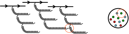
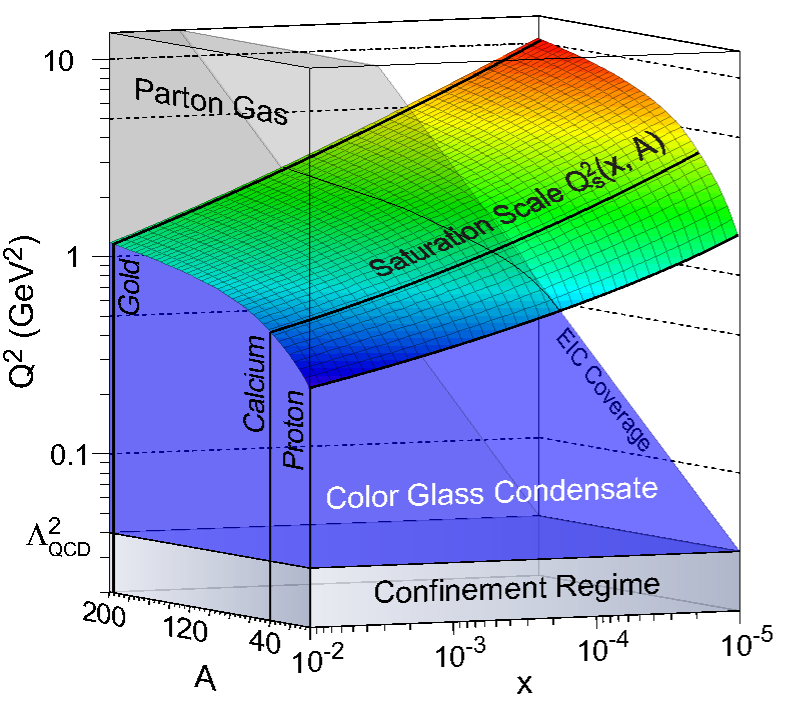
Figure 8: Left: gluon cascades from a valence quark in a hadron. Right: saturation domain as a function of the value of $x$ and the atomic number $A$ of the nucleus[21].

At small $Y$, i.e. in the dilute regime where ${\boldsymbol{T}}$ is small, one probes the valence quarks only. At larger values of $Y$, the dipole can interact not only with the valence quarks, but also with gluons radiated from the valence quarks. At even larger values of $Y$, these gluons themselves emit more gluons, in ladder-like diagrams. In this regime, the growth of the number of gluons is exponential in the rapidity $Y$. This very fast growth continues until the gluon density becomes too large. Roughly speaking, when the areal gluon density in the transverse plane multiplied by the cross-section for the recombination of two gluons by the process $gg\to g$ becomes of order one, then the nonlinearities become important. Their effect is to tame the growth of the gluon density, so that the scattering amplitude ${\boldsymbol{T}}$ remains bounded. This phenomenon is known as gluon saturation.

The criterion for the onset of gluon saturation can be expressed in terms of the resolution scale $Q$ at which the gluons are observed. It reads

$$\underbrace{\alpha_{s}Q^{-2}}_{\sigma_{gg\to g}}\;\times\;\underbrace{A^{-2/3}xG(x,Q^{2})}_{\mbox{\scriptsize surface density}}\;\geq\;1\;,$$ (41)

where $A$ is the atomic number in the case the target is a nucleus (otherwise it is unity). This inequality can be rearranged into

$$Q^{2}\leq\underbrace{{Q_{s}^{2}}\equiv\frac{{\alpha_{s}}{xG(x,Q_{s}^{2})}}{{A^{2/3}}}}_{\mbox{\scriptsize saturation momentum}}\;\sim\;{A^{1/3}}{x^{-0.3}}\;.$$ (42)

The right hand side of this inequality is called the saturation momentum. The effects of gluon saturation are important below this scale, and are therefore more visible when this scale is large. It is easy to estimate the $A$ and $x$ dependence of the saturation momentum. Because $Q_{s}^{2}$ is the ratio of a quantity proportional to the volume of the target by an area, it should scale like $A^{1/3}$. Its $x$ dependence can be inferred from the behavior of the gluon distribution in nucleons at small $x$: it grows like a power of $1/x$, the numerical value $\sim 0.3$ of the exponent being extracted from HERA data for instance. The value of the saturation momentum as a function of $x$ and $A$ is shown in the right plot of the figure 8, and the dense/saturated regime comprises the volume under the surface.

Note that the eq. (40) derived here resums only the leading log terms, since it is based only on the kernel at one loop. At this order, there is no running of the coupling constant. This effect arises via some parts of the two-loop kernel, that involve the beta function. These corrections are known by now[22, 23, 24, 25] and play an important role in reaching a good agreement with experimental data[26, 27, 28, 29].

2.5 Target average

Until now, we have treated the target as a given patch of color field, produced by the constituents of the target, that are static over the timescale of the collision due to Lorentz time dilation. However, this picture implies that details of this color field depend of the precise configuration (position, color, …) of the constituents of the target at the time of the collisions, that of course we do not know. Since this configuration changes from collision to collision, so does the target field. Therefore, instead of a single target field, one should instead have in mind an ensemble of such fields, corresponding to all the possible configurations of the constituents of the target. This means that all the quantities we have so far evaluated in a given target field should in fact be averaged over this ensemble of target fields,

$${{\boldsymbol{T}}}\quad\to\quad\left<{{\boldsymbol{T}}}\right>\;.$$ (43)

When performing this average at the level of the BK equation, we naturally get

$$\frac{\partial\,\left<{{\boldsymbol{T}}({\boldsymbol{x}}_{\perp},{\boldsymbol{y}}_{\perp})}\right>}{\partial{Y}}=\frac{{\alpha_{s}N_{c}}}{2\pi^{2}}\int d^{2}{\boldsymbol{z}}_{\perp}\;\frac{({\boldsymbol{x}}_{\perp}-{\boldsymbol{y}}_{\perp})^{2}}{({\boldsymbol{x}}_{\perp}-{\boldsymbol{z}}_{\perp})^{2}({\boldsymbol{y}}_{\perp}-{\boldsymbol{z}}_{\perp})^{2}}$$

$$\times\Big{\{}\!\!\left<{{\boldsymbol{T}}({\boldsymbol{x}}_{\perp},{\boldsymbol{z}}_{\perp})}\right>+\left<{{\boldsymbol{T}}({\boldsymbol{z}}_{\perp},{\boldsymbol{y}}_{\perp})}\right>-\left<{{\boldsymbol{T}}({\boldsymbol{x}}_{\perp},{\boldsymbol{y}}_{\perp})}\right>-\left<{{\boldsymbol{T}}({\boldsymbol{x}}_{\perp},{\boldsymbol{z}}_{\perp})}{{\boldsymbol{T}}({\boldsymbol{z}}_{\perp},{\boldsymbol{y}}_{\perp})}\right>\!\!\Big{\}}\,.$$ (44)

The trouble with this equation is that it is no longer a closed equation, since the evolution with $Y$ of the quantity $\left<{{\boldsymbol{T}}}\right>$ depends on the value of a new quantity $\left<{{\boldsymbol{T}}}{{\boldsymbol{T}}}\right>$. By the same method used to derive the evolution equation for $\left<{{\boldsymbol{T}}}\right>$, we could derive an evolution equation for $\left<{{\boldsymbol{T}}}{{\boldsymbol{T}}}\right>$, but its right hand side would contain the average value of an object containing three factors ${\boldsymbol{T}}$, and so on. Therefore, instead of a single closed equation, we have now an infinite hierarchy of nested equations, known as the Balitsky hierarchy[30].

There is an approximation of the above hierarchy of equations, that leads us back to the original Balitsky-Kovchegov equation. This approximation amounts to assuming that the average of a product of two dipole operators factorizes into the product of their averages,

$$\left<{{\boldsymbol{T}}\,{\boldsymbol{T}}}\right>\approx\left<{{\boldsymbol{T}}}\right>\,\left<{{\boldsymbol{T}}}\right>\;.$$ (45)

Obviously, if this is true, then the first equation of the hierarchy is nothing but the BK equation. This mean-field approximation is believed to be valid for large targets such as nuclei, and in the limit of a large number of color. Although subject to this approximation, the BK equation is widely used in phenomenological applications because of its simplicity.

2.6 Geometrical scaling

The BK equation leads to an interesting property of the DIS total cross-section, called geometrical scaling. Firstly, let us write the $\gamma^{*}$-target cross-section as follows,

$$\sigma_{\gamma^{*}T}=\int_{0}^{1}dz\int d^{2}{\boldsymbol{r}}_{\perp}\left|\psi({\boldsymbol{q}}|z,{\boldsymbol{r}}_{\perp})\right|^{2}\sigma_{\rm dipole}({\boldsymbol{r}}_{\perp})\;,$$ (46)

with

$$\sigma_{\rm dipole}({\boldsymbol{r}}_{\perp})\equiv{2}\int d^{2}{\boldsymbol{X}}_{\perp}\;{\boldsymbol{T}}({\boldsymbol{X}}_{\perp}+\frac{{\boldsymbol{r}}_{\perp}}{2},{\boldsymbol{X}}_{\perp}-\frac{{\boldsymbol{r}}_{\perp}}{2})\;.$$ (47)

$\psi({\boldsymbol{q}}|z,{\boldsymbol{r}}_{\perp})$ is the light-cone wavefunction for a virtual photon of momentum ${\boldsymbol{q}}$ splitting into a $q\overline{q}$ pair or transverse size ${\boldsymbol{r}}_{\perp}$, where the quarks carries the fraction $z$ of the longitudinal momentum of the photon. This object is a purely electromagnetic quantity (at least at leading order), and is not interesting from the point of view of strong interactions, that are all contained in the dipole cross-section defined in eq. (47). This equation defines the total cross-section between the $q\overline{q}$ pair and the target, expressed in terms of the forward scattering amplitude thanks to the optical theorem. Thus, the BK equation tells us about the rapidity dependence (i.e. the $x$ dependence since $Y\equiv\log(1/x)$) of the DIS cross-section.

For the sake of the argument, let us assume translation and rotation invariance, and define

$${N(k_{\perp})}\equiv 2\pi\int d^{2}{\boldsymbol{x}}_{\perp}\;e^{i{\boldsymbol{k}}_{\perp}\cdot{\boldsymbol{x}}_{\perp}}\;\frac{\left<{{\boldsymbol{T}}(0,{\boldsymbol{x}}_{\perp})}\right>}{x_{\perp}^{2}}\;.$$ (48)

From the Balitsky-Kovchegov equation for $\left<{{\boldsymbol{T}}}\right>$, we obtain the following equation for ${N}$

$$\frac{\partial{N(k_{\perp})}}{\partial{Y}}=\frac{{\alpha_{s}N_{c}}}{\pi}\Big{[}{\chi(-\partial_{L})}{N(k_{\perp})}-{N^{2}(k_{\perp})}\Big{]}\;,$$ (49)

where we denote

$${L}\equiv{\ln(k^{2}/k_{0}^{2})}$$

$${\chi(\gamma)}\equiv{2\psi(1)-\psi(\gamma)-\psi(1-\gamma)}$$

$$\psi(z)\equiv\frac{d\ln\Gamma(z)}{dz}\;.$$ (50)

($\Gamma(z)$ is Euler’s Gamma function.) The form (49) of the BK equation is particularly simple, because its nonlinear term is just the square of the function $N$.

The function ${\chi(\gamma)}$ has a minimum at $\gamma=1/2$. Eq. (49) can be approximated by expanding ${\chi(\gamma)}$ to quadratic order around the minimum. This amounts to keeping only derivatives with respect to $L$ up to second order, i.e. to a diffusion approximation. The physical content of this equation becomes more transparent if one also introduces the following variables,

$${t}\sim{Y}$$

$${z}\sim L+\frac{{\alpha_{s}N_{c}}}{2\pi}\chi^{\prime\prime}(1/2)\;{Y}\;,$$ (51)

in terms of which eq. (49) becomes[31, 32, 33]

$${\partial_{t}}{N}={\partial_{z}^{2}}{N}+{N}-{N}^{2}\;.$$ (52)

This equation is known as the Fisher-Kolmogorov-Petrov-Piscounov (FKPP) equation, and it describes the physics of reaction-diffusion processes. These are processes involving a certain entity $A$ that can do the following:

• An entity $A$ can hop from a location to neighboring locations. This is described by the diffusion term in the right hand side of eq. (52).

• An entity $A$ can split into two, increasing the population by one unit. This is described by the $+N$ term.

• Two of these entities can merge into a single one, reducing their population by one unit. This is described by the term $-N^{2}$.

The FKPP equation has two fixed points, $N=0$ which is unstable, and $N=1$ which is a stable fixed point. Note that the loss term, $-N^{2}$, is essential for the existence of this stable fixed point. Moreover, for rather generic initial conditions, the solutions of the FKPP equation are known to behave like traveling waves at asymptotic times

$${N}(t,z)\mathrel{\mathop{\kern 0.0pt\sim}\limits_{t\to+\infty}}{N}(z-2t)\;.$$ (53)

In other words, these solutions propagate in the $+z$ direction at the constant velocity $dz/dt=2$, and instead of depending separately on $z$ and $t$, they depend only on the combination $z-2t$. Going back to the dipole scattering amplitude ${\boldsymbol{T}}$, we see that it does not depend separately on $Y$ and on the dipole size ${\boldsymbol{r}}_{\perp}$, but on the combination $Q_{s}(Y){\boldsymbol{r}}_{\perp}$, where $Q_{s}(Y)$ has the following $Y$ dependence

$${Q_{s}^{2}(Y)}=k_{0}^{2}\;{Y}^{-\frac{3}{2(1-\bar{\gamma})}}\;e^{{\overline{\alpha}_{s}\chi^{\prime\prime}(\frac{1}{2})(\frac{1}{2}-\bar{\gamma})}{Y}}\;.$$ (54)

This quantity is nothing but the saturation momentum introduced by a simple semi-quantitative argument earlier. Here, we see it emerge dynamically from the evolution equation itself. This is a major feature of gluon saturation: the ability to generate a dimensionful scale is a consequence of the nonlinear aspect of the saturation phenomenon. Moreover, thanks to the fact that this scale increases with $Y$, i.e. with the energy scale, one may hope that gluon saturation falls in the realm of weakly coupled physics at sufficiently high energy.

And at the level of the $\gamma^{*}$-target cross-section, this implies that the cross-section depends only on $Q^{2}/Q_{s}^{2}(Y)$, rather than $Q^{2}$ and $Y$ separately (this is strictly true assuming that we neglect any other dimensionful parameters in the problem, such as the quark masses that enter in the virtual photon wavefunction $\psi$ – this is legitimate for the light $u,d$ and $s$ quarks). This scaling property of the DIS total cross-section has been observed in experimental data, as shown in the right plot of the figure 9.

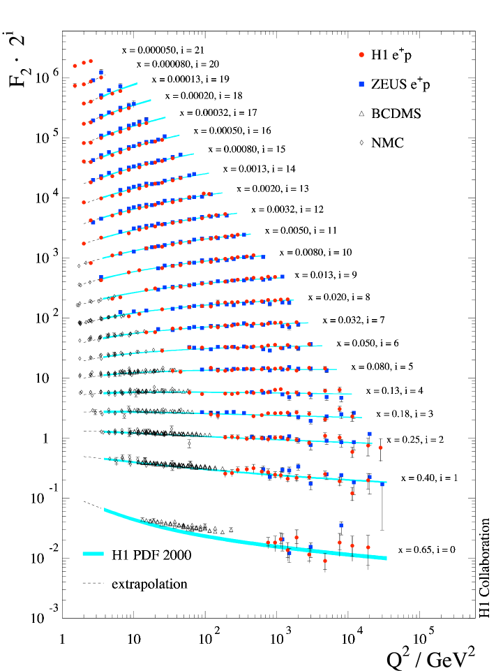
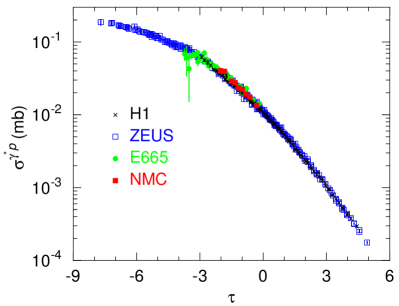
Figure 9: DIS data at HERA. Left: displayed conventionally as a function of $x$ and $Q^{2}$. Right: displayed as a function of $\tau\equiv Q^{2}/Q_{s}^{2}(x)$ [34, 35].

What makes gluon saturation a satisfying explanation of this phenomenon is that geometrical scaling is a very robust consequence of evolution equations with a nonlinear term that tames the growth of the amplitude, since any realistic initial condition falls leads to traveling wave solutions. Interestingly, the scaling shown in the right plot of the figure 9 also works for DIS off nuclei[36], provided one scales the saturation momentum by the appropriate factor $A^{1/3}$ (see the NMC data points). For large nuclei like the ones employed in heavy ion collisions (Gold at RHIC and Lead at the LHC), the nuclear enhancement of the saturation momentum is $A^{1/3}\approx 6$. From fits to existing data on deep inelastic scattering on various targets, one can get a more precise idea of the numerical value of the saturation momentum[37, 38] (this is how $Q_{s}$ has been obtained in the figure 8).

3 Introduction to the Color Glass Condensate

3.1 Other elementary reactions

In the previous section, we have studied Deep Inelastic Scattering and its energy evolution from the point of view of the projectile (in this case, the virtual photon). When going to NLO, the correction was applied to the $q\overline{q}$ dipole, while the target field was held fixed. In other words, all the energy evolution was applied to the dipole. This is perfectly legitimate: since cross-sections are Lorentz invariant objects, they do not depend on the frame. The kind of calculation we have performed in the previous section amounts to observing the reaction in a frame where the target is nearly at rest, and the boost to go to higher energy is applied entirely to the virtual photon. In the case of DIS, the interest in doing so is obvious: the target is very complicated (a nucleon or a nucleus), while the projectile is a rather elementary object (a virtual photon). Thus it seemed natural to look at the energy evolution by boosting the object we understand best.

There is another situation where one can proceed in this way, that involves colliding a dilute projectile on a dense target. This is the case for instance in proton-nucleus collisions, at forward rapidities in the direction of the proton beam. In this kinematical configuration, one probes the dilute regime of the proton, and the dense regime of the nucleus.

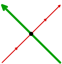
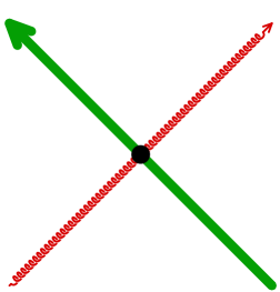
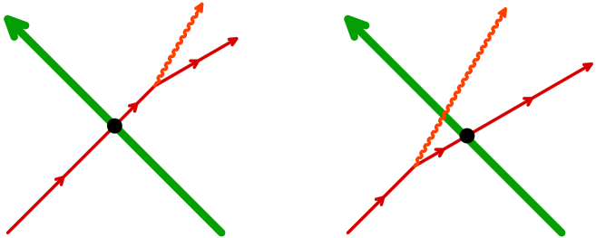
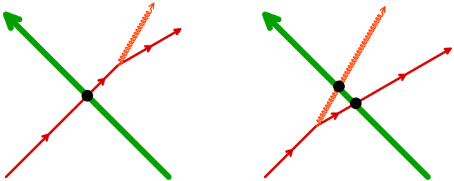
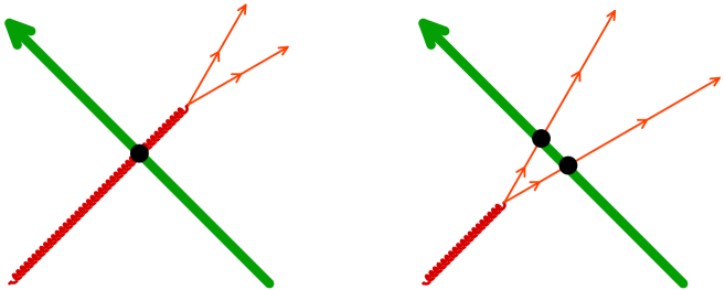
Figure 10: Examples of elementary processes involving a projectile quark or gluon and the field of a target nucleus. Each black dot represents the Wilson line associated with the eikonal scattering of the corresponding parton.

In this case, the proton can be describe as a dilute beam of quarks or gluons whose flux is given by the usual parton distributions, and the elementary reactions we must consider are the interactions between a quark or a gluon and the field of the target nucleus. Examples of processes[39, 40, 41, 42, 43, 44, 45, 46, 47, 48, 49, 50, 51, 52, 53, 54, 55, 56, 57, 58, 58, 59, 60, 61, 62, 63, 64] that have been evaluated in this way are represented in the figure 10.

However, this approach suffers from a serious limitation, since it is practical only when the projectile is much simpler than the target. For symmetric collisions, such as nucleus-nucleus collisions. In this case, there is no advantage in treating differently the two nuclei. In fact, doing so is arguably rather unnatural. As we shall see shortly, the Color Glass Condensate description of gluon saturation allows a perfectly symmetric description of the two nuclei in these collisions.

3.2 Color sources and quantum fields

Before we turn to the study of nucleus-nucleus collisions, let us consider again DIS, but this time from the point of view of the target, i.e. when we go to higher energy, we apply the boost to the target while leaving the projectile wavefunction unchanged. In the previous, we simply assumed that the target can be represented by a certain ensemble of color field configurations, that we did not specify. If we adopt the point of view that consists in applying the boost to the target, then this ensemble of fields must change with energy for the cross-section to have the correct energy dependence.

At the basis of the Color Glass Condensate framework is the fact that the fast partons of a hadron or nucleus suffer Lorentz time dilation and therefore do not evolve during the short duration of a collision. They can thus be considered as time independent objects moving at the speed of light along the light-cone, and the only relevant information we need to know about them is the color charge they carry. This can be encoded in a color current of the form

$$J^{\mu}_{a}={\delta^{\mu+}}{\rho_{a}(x^{-},{\boldsymbol{x}}_{\perp})}\;.$$ (55)

This formula keeps only the longitudinal component of the current (the $+$ component in light-cone coordinates), and neglects all the other components, because only this component is enhanced by the Lorentz factor. The lack of $x^{+}$ dependence stems from the assumption that these color charges are time independent. The function $\rho_{a}$ describes the spatial distribution of these color charges, both in $x^{-}$ and in ${\boldsymbol{x}}_{\perp}$. Note that the support of its $x^{-}$ dependence is very narrow, due to Lorentz contraction. At leading order, the target field can be obtained by solving the Yang-Mills equation with the source $J^{\mu}$,

$$\big{[}D_{\mu},F^{\mu\nu}\big{]}=J^{\nu}\;.$$ (56)

In the Lorenz gauge, defined by $\partial_{\mu}A^{\mu}=0$, this equation can be solved analytically for the above current, and one obtains

$$A^{-}=A^{i}=0\quad,\quad A^{+}(x)=-\frac{1}{{\boldsymbol{\nabla}}_{\perp}^{2}}\;\rho(x^{-},{\boldsymbol{x}}_{\perp})\;.$$ (57)

Therefore, specifying the ensemble of target fields is equivalent to specifying the ensemble of the functions $\rho$. Thus, the CGC framework must be supplemented by a probability distribution $W[\rho]$.

The ideas behind the Color Glass Condensate originate in the McLerran-Venugopalan model[65, 66, 67] that, in addition to the description of a dense object in terms of classical color sources, also argued that their distribution $W[\rho]$ should be nearly Gaussian, with only local correlations,

$$\left<\rho_{a}(x^{-},{\boldsymbol{x}}_{\perp})\rho_{b}(y^{-},{\boldsymbol{y}}_{\perp})\right>=\mu^{2}\delta^{ab}\delta(x^{-}-y^{-})\delta({\boldsymbol{x}}_{\perp}-{\boldsymbol{y}}_{\perp})\;.$$ (58)

The justification of this model is that, in a highly Lorentz contracted nucleus, there is a large density of color charges at each impact parameter. The charges from different nucleons are uncorrelated, and thus by the central limit theorem, the resulting distribution should be approximately Gaussian for a large nucleus. The locality of the correlations is also a consequence of the fact that charges in different nucleus are not correlated.

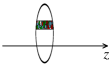
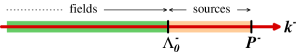
Figure 11: Left: illustration of the McLerran-Venugopalan model for a large nucleus. Right: separation in longitudinal momentum between fields and sources (here for a target moving in the $-z$ direction – hence the cutoff on the $k^{-}$ component of the momentum).

3.3 Cutoff dependence and renormalization group evolution

The justification for treating the constituents of the target as static color sources is Lorentz time dilation. Arguably, this is only justified if these partons have a large enough longitudinal momentum. The partons that are too slow must be treated in terms of the usual gauge fields (if they are gluons). Therefore, the CGC should be viewed as an effective theory with a cutoff $\Lambda^{+}$, such that

• Partons with $k^{+}>\Lambda^{+}$ are treated as static sources, via eq. (55).

• Partons with $k^{+}<\Lambda^{+}$ are treated as standard quantum fields.

Because these two types of degrees of freedom have well separated longitudinal momenta, the interactions between them can be approximated by an eikonal coupling $J_{\mu}A^{\mu}$, and the action that describes the complete effective theory is

$${\cal S}=\underbrace{-\frac{1}{4}\int F_{\mu\nu}F^{\mu\nu}}_{\mbox{Yang-Mills}}+\underbrace{\int{J^{\mu}}{A_{\mu}}}_{\mbox{fast partons}}.$$ (59)

In the CGC framework, the expectation value of an observable is obtained by first computing the observable for a fixed configuration $\rho$ of the color sources of the target, and then by averaging it with the distribution $W[\rho]$,

$$\left<{{\boldsymbol{\cal O}}}\right>={\int\left[D\rho\right]\;{W[\rho]}\;{{\boldsymbol{\cal O}}}[\rho]}\;.$$ (60)

The cutoff $\Lambda^{+}$ that has been introduced to separate the fast and the slow partons is arbitrary, and observable quantities should not depend on it. At leading order, this is always the case. But when one computes loop corrections, the cutoff enters in the calculation as an upper limit on the longitudinal momentum that runs in the loop, in order to prevent the quantum modes that are integrated in the loop to duplicate modes that are already introduced via the static source $\rho_{a}$. In general, this leads to a logarithmic dependence of the loop corrections on the cutoff $\Lambda^{+}$ [68]. The only way to have $\Lambda$-independent observables at the end of the day is to let the distribution $W[\rho]$ depend itself on $\Lambda$, precisely in such a way that the two $\Lambda$ dependences cancel,

$$W[\rho]\to W_{{}_{\Lambda}}[\rho]\;.$$ (61)

Moreover, it turns out that this can be achieved with the same distribution $W_{{}_{\Lambda}}[\rho]$ for a wide range of different observables, with a $\Lambda$ dependence governed by the so-called JIMWLK equation[69, 70, 71, 72, 73, 74, 75, 76], of the form

$$\frac{\partial W_{{}_{\Lambda}}}{\partial\log\Lambda}={\cal H}\,W_{{}_{\Lambda}}\;,$$ (62)

where ${\cal H}$ (the JIMWLK Hamiltonian) is a quadratic operator in functional derivatives with respect to $\rho$. Note that the $\Lambda$ dependence is often traded for a rapidity dependence, by using $Y\equiv\log(\Lambda)$. The evolution equation (62) can be seen as a renormalization group equation, that describes how the color charge content of the target changes as one changes the longitudinal momentum $\Lambda$ down to which they are considered. When the cutoff $\Lambda$ is large, and close to the longitudinal momentum of the target, only its valence partons are included in the description in terms of $\rho$. Lowering $\Lambda$ means that one includes in this effective description more and more soft modes (sea partons).

The JIMWLK equation does not predict by itself what the distribution $W_{{}_{\Lambda}}[\rho]$ is for a given target, only how it changes when on lowers the cutoff. It must be supplemented by an initial condition at some $\Lambda_{0}$ in order to lead to definite results. This initial condition is by essence non-perturbative, and must be modelled. When the evolution of the distribution $W_{{}_{\Lambda}}[\rho]$ is considered, the status of the McLerran-Venugopalan model changes a bit, because the Gaussian distribution proposed by the MV model is not a fixed point of the JIMWLK equation. Instead, the MV model is often viewed as a plausible initial condition for a large nucleus at large cutoff (i.e. close to the valence region of the target).

Although it is necessary to specify an initial condition in order to solve the JIMWLK equation, it should be stressed that its solutions have a universal scaling property when evolved far enough from the initial cutoff scale: the equation generates an intrinsic momentum scale, the saturation momentum $Q_{s}$, and in this scaling regime all the correlation functions of Wilson lines depend on the transverse coordinates only via combinations such as $Q_{s}{\boldsymbol{x}}_{\perp}$. This scaling of the solutions of the JIMWLK equation is what led to asymptotic traveling wave solutions for the BK equation. This behavior of the solutions mean that they tend to forget the details of their initial condition, if evolved sufficiently far from the starting scale. This suggests that predictions of the CGC should be less sensitive to the model employed for the initial condition when applied to the study of collisions at very high energy.

3.4 Relationship between the Balitsky’s and CGC formulations

The correspondence between Balitsky’s hierarchy and the CGC formulation can be summarized by the following identity,

$$\left<{{\boldsymbol{\cal O}}}\right>_{{}_{Y}}=\underbrace{\int\left[D\rho\right]\;{W_{0}[\rho]}\;{{\boldsymbol{\cal O}}}_{{}_{Y}}[\rho]}_{\mbox{\scriptsize Balitsky's description}}=\underbrace{\int\left[D\rho\right]\;{W_{{}_{Y}}[\rho]}\;{{\boldsymbol{\cal O}}}_{0}[\rho]}_{\mbox{\scriptsize CGC description}}\;.$$ (63)

In the Balitsky’s approach, the rapidity dependence is obtained by applying a boost to the observable, while the distribution of sources is kept unchanged. In the CGC approach, the observable is a fixed functional of the sources, and the boost leads to a change in the distribution of the sources. In the simple case of collisions between an elementary projectile and a dense target, where observables can be expressed in terms of Wilson lines of the target field, the equivalence between these two points of view follows from the existence of a universal operator ${\cal H}$ such that

$$\frac{\partial{{\boldsymbol{\cal O}}}_{{}_{Y}}[\rho]}{\partial{Y}}={\cal H}\left[\rho,\frac{\delta}{\delta\rho}\right]\;\;{{\boldsymbol{\cal O}}}_{{}_{Y}}[\rho]\;.$$ (64)

Moreover, this operator is self-adjoint, which means that one can “integrate by parts” and transpose its action from the observable to the distribution $W[\rho]$, leading to the JIMWLK evolution equation.

3.5 Example : DIS in the CGC framework

As an illustration of the use of the CGC, let us reconsider Deep Inelastic Scattering in this framework (see the figure 12). We present here only a sketch of the calculation, but not the details[77, 78].

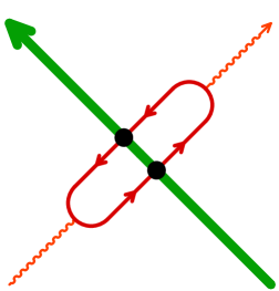
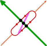
Figure 12: Deep inelastic scattering in the CGC framework. The green arrow represents the trajectory of the target, and the support of its color sources. Left: Leading Order: the virtual photon fluctuates into a $q\overline{q}$ dipole that scatters off the color field of the target. Right: Next to Leading Order: the photon fluctuates into a $q\overline{q}g$ state.

At LO, the photon must fluctuate into a $q\overline{q}$ dipole in order to interact with the field of the target. As with the BK approach, the forward scattering amplitude of this dipole off the target can be expressed in terms of Wilson lines,

$${{\boldsymbol{T}}_{{}_{\rm LO}}({\boldsymbol{x}}_{\perp},{\boldsymbol{y}}_{\perp})} = 1-\frac{1}{N_{c}}\,{\rm tr}\,({{U({\boldsymbol{x}}_{\perp})U^{\dagger}({\boldsymbol{y}}_{\perp})}})$$

$$U({\boldsymbol{x}}_{\perp}) = {\rm P}\,\exp i{g}\int dz^{+}\,{{\cal A}^{-}(z^{+},{\boldsymbol{x}}_{\perp})}\;,$$ (65)

and the main difference resides in the fact that the target field is not arbitrary but obtained by solving the Yang-Mills equation

$$\left[{{\cal D}_{\mu}},{{\cal F}^{\mu\nu}}\right]={\delta^{\nu-}}\,{\rho(x^{+},{\boldsymbol{x}}_{\perp})}\;.$$ (66)

Then the cross-section is obtained by averaging over all the configurations of the color source $\rho$, with the distribution $W[\rho]$. At LO, the difference with the BK point of view is purely semantic, since we are simply trading the (arbitrary) distribution of the target fields for the (arbitrary) distribution of the color sources.

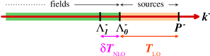
Figure 13: Infinitesimal step in the cutoff evolution, from $\Lambda_{0}$ to $\Lambda_{1}$.

At NLO, one must now consider corrections such as the one represented in the right part of the figure 12 (there are several graphs, only one of them is represented there). The longitudinal momentum of the gluon in the calculation of these corrections should be limited at the upper value $\Lambda_{0}^{-}$, to avoid over-counting modes that are already included via the sources $\rho$. In practice, it is more convenient to compute only the correction $\delta T_{{}_{\rm NLO}}$ to the scattering amplitude due to the field modes in a small strip $\Lambda_{1}^{-}<k^{-}<\Lambda_{0}^{-}$. The important part in this discussion are the terms that have logarithm divergences when $\Lambda_{1}^{-}\ll\Lambda_{0}^{-}$. One can show that they take the following form,

$${\delta{\boldsymbol{T}}_{{}_{\rm NLO}}({\boldsymbol{x}}_{\perp},{\boldsymbol{y}}_{\perp})}=\ln\left(\frac{\Lambda_{0}^{-}}{\Lambda_{1}^{-}}\right)\;{{\cal H}}\;{{\boldsymbol{T}}_{{}_{\rm LO}}({\boldsymbol{x}}_{\perp},{\boldsymbol{y}}_{\perp})}\;,$$ (67)

where ${\cal H}$ is an operator that acts on the $\rho$’s. Besides the fact that they depend on an unphysical cutoff, these logarithms question the validity of the perturbative expansion. Indeed, the NLO corrections are suppressed by one power of the coupling constant $\alpha_{s}$ compared to the LO result, but the appearance of these possibly large logarithms can compensate the smallness of the coupling. This is why one should consider only a small slice of longitudinal momenta at a time. It turns out that these logarithms can be hidden by averaging over the color sources, thanks to the identity

$$\Big{<}{{\boldsymbol{T}}_{{}_{\rm LO}}}+{\delta{\boldsymbol{T}}_{{}_{\rm NLO}}}\Big{>}_{\Lambda_{0}^{-}}=\Big{<}{{\boldsymbol{T}}_{{}_{\rm LO}}}\Big{>}_{\Lambda_{1}^{-}}\;,$$ (68)

where we use the shorthand

$$\big{<}\cdots\big{>}_{\Lambda}\equiv\int[D\rho]\;W_{{}_{\Lambda}}[\rho]\;\cdots\;,$$ (69)

provided the distributions of sources at the scales $\Lambda_{0}^{-}$ and $\Lambda_{1}^{-}$ are related by

$$W_{\Lambda_{1}^{-}}\equiv\Big{[}1+\ln\left(\frac{\Lambda_{0}^{-}}{\Lambda_{1}^{-}}\right)\;{{\cal H}}\Big{]}\;W_{\Lambda_{0}^{-}}\;.$$ (70)

The meaning of eq. (68) is that the sum of the LO+NLO contributions in the original effective theory (that has its cutoff at the scale $\Lambda_{0}^{-}$) is equivalent to the LO only in a new effective theory that has its cutoff at the lower scale $\Lambda_{1}^{-}$, and a new distribution of sources given by eq. (70). Note that eq. (70) is nothing but the JIMWLK equation for an infinitesimal change of the cutoff scale. Moreover, the right hand side of eq. (68) has no dependence on the former scale $\Lambda_{0}^{-}$. This means that in the left hand side, this dependence must cancel between the NLO contribution and the scale dependence of the distribution $W[\rho]$.

The previous process, by which we integrated out the logarithms coming from a small slice of field modes, can be repeated indefinitely by considering a sequence of lower and lower cutoffs,

$$\cdots<\Lambda_{n}^{-}<\cdots<\Lambda_{1}^{-}<\Lambda_{0}^{-}\;.$$ (71)

At each step, new logarithms are generated, that can be absorbed by defining a new effective theory at the lower scale $\Lambda_{n+1}^{-}$ and a new distribution of sources at this scale. The dependence on the cutoff at the previous scale $\Lambda_{n}^{-}$ disappears in this process. We must repeat this procedure until we reach a cutoff scale which is lower than all the physically relevant longitudinal momentum scales: at this point, lowering the cutoff further only introduces new sources that are too slow to be relevant in the observable under consideration – the observable does not depend on these sources, and thus becomes independent of the cutoff.

4 Factorization in high-energy hadronic collisions

4.1 Introduction

In the previous section, we have introduced the Color Glass Condensate effective theory, and illustrated it by considering again the example of Deep Inelastic Scattering. In this context, the CGC is a mere rephrasing of the physics that was already present in Balitsky’s hierarchy. Roughly speaking, the CGC puts the emphasis on the energy evolution of the distribution that describes the target, rather than on radiative corrections to the operator that is being measured, but the end result is exactly the same.

The situation is qualitatively different in the case of nucleus-nucleus collisions. In this case, it would be highly desirable to have a framework in which the projectile and target can be treated on the same footing, and the CGC appears as a good candidate for achieving this. In the CGC framework, we expect that each of the nuclei will be described by static color sources $\rho_{1}$ and $\rho_{2}$, moving in opposite directions along the light-cone, with their respective distributions $W_{1}[\rho_{1}]$ and $W_{2}[\rho_{2}]$.

In several works[79, 80, 81, 82, 83, 84, 85, 86, 87, 88], the CGC has been used as follows in order to compute observables in heavy ion collisions :

• Pick randomly two color sources $\rho_{1}$ and $\rho_{2}$ (one for each nucleus), for instance by using the Gaussian distributions encountered in the MV model.

• Solve (numerically) the classical Yang-Mills equation with two sources,

  $$\left[{{\cal D}_{\mu}},{{\cal F}^{\mu\nu}}\right]={\delta^{\nu-}}\,{\rho_{1}}+\delta^{\mu+}\,\rho_{2}\;,$$ (72)

  with an initial condition such that the color field vanishes at $x^{0}\to-\infty$.

• Evaluate the observable of interest on the classical color field ${\cal A}^{\mu}$ obtained by solving the previous equation. For instance, the gluon spectrum is obtained as

  $$\left.\frac{d{{{N_{1}}}}}{dYd^{2}{\boldsymbol{p}}_{\perp}}\right|_{{}_{\rm LO}}=\frac{1}{16\pi^{3}}\int_{x,y}\;{e^{ip\cdot(x-y)}}\;\square_{x}\square_{y}\;\sum_{\lambda}\epsilon^{\mu}_{\lambda}\epsilon^{\nu}_{\lambda}\;\;{{\cal A}_{\mu}(x)}{{\cal A}_{\nu}(y)}\;.$$

• Repeat these steps in order to perform a Monte-Carlo average over the distributions for $\rho_{1}$ and $\rho_{2}$.

As an illustration, we show in the figure 14 some numerical results for the single inclusive spectrum of the gluons produced in a nucleus-nucleus collision, obtained by following this procedure.

Figure 14: Transverse momentum dependence of the single inclusive gluon spectrum[83].

The goal of this section is to provide a theoretical justification for the above procedure, and in particular to answer the following questions :

• Does it correspond to the leading term in an expansion in powers of the coupling constant?

• What is the justification for the use of retarded boundary conditions?

• In the case of a collision between two nuclei, can one still absorb the logarithms that arise in loop corrections by letting the distributions $W_{1}[\rho_{1}]$ and $W_{2}[\rho_{2}]$ evolve according to the JIMWLK equation?

4.2 Power counting

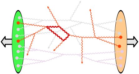
Figure 15: Typical connected graph in a nucleus-nucleus collision described in the CGC framework. In this representation, the circular dots represent insertions of the sources $\rho_{1}$ or $\rho_{2}$.

Before we can start answering these questions, we need a way to assess the order of magnitude of a given graph[89, 90]. Typical graphs in a nucleus-nucleus collisions are made of several disconnected components (see the graph on the right of the figure 6). In order to perform this power counting, it is sufficient to consider only one of these connected components, as illustrated in the figure 15. In this representation, the circular dots represent insertions of the sources $\rho_{1}$ or $\rho_{2}$. In the saturated regime, their contribution to the power counting is $g^{-1}$, since the gluon occupation number, proportional to $\rho^{2}$, should be of order $g^{-2}$. In addition, three-gluon vertices bring one power of $g$ and four-gluon vertices a factor $g^{2}$.

With these rules, one obtains the following order of magnitude for a connected graph such as the one represented in the figure 15 :

$$\frac{1}{g^{2}}\,g^{n_{{}_{E}}+2n_{{}_{L}}}\;,$$ (73)

where $n_{{}_{E}}$ is the number of external gluons (the gluon lines terminated by an arrow in the figure 15) and $n_{{}_{L}}$ the number of independent loops in the graph.

Interestingly, the order of the graph does not depend on the number of internal lines and on the number of sources $\rho_{1,2}$ attached to the graph. The latter property is specific of the dense regime, where the sources are of order $g^{-1}$. Indeed, each insertion of a source necessarily brings a factor $g$ for the vertex at which this source is attached to the graph; this vertex cancels the $g^{-1}$ coming from the source and therefore inserting a source in the graph does not cost any power of $g$. This means that, for graphs with a fixed number of external lines and a fixed number of loops, there is an infinity of topologies of the same order in $g$ that differ in the number of sources they contain. Thus, computing any observable in the CGC framework, even at Leading Order, requires that one resums this infinite series of terms.

For instance, the inclusive gluon spectrum has the following expansion

$$\frac{d{N_{1}}}{d^{3}{\boldsymbol{p}}}=\frac{1}{{g^{2}}}\;\Big{[}c_{0}+c_{1}\,{g^{2}}+c_{2}\,{g^{4}}+\cdots\Big{]}\;,$$ (74)

where the coefficients $c_{0},c_{1},\cdots$ are themselves series that resum all orders in $(g\rho_{{}_{1,2}})^{n}$. For instance,

$$c_{0}=\sum_{n=0}^{\infty}c_{0,n}\,({g}{\rho_{{}_{1,2}}})^{n}\;.$$ (75)

Our goal in the rest of this section is to calculate the complete zeroth order term, ${c_{0}/g^{2}}$, and a subset of the higher order terms.

4.3 Bookkeeping

Among the observables that one could possibly consider, the inclusive observables are especially simple because they do not veto any final state. This is the case for instance of the single inclusive gluon spectrum, defined in terms of the transition amplitudes as

$$\frac{dN_{1}}{d^{3}{{\boldsymbol{p}}}}\sim\sum_{n=0}^{\infty}(n+1)\int\frac{1}{(n+1)!}\Big{[}\underbrace{d\Phi_{1}\cdots d\Phi_{n}}_{n\mbox{\scriptsize\ part. phase-space}}\Big{]}\;\Big{|}\big{<}{{\boldsymbol{p}}}{\boldsymbol{p}}_{1}\cdots{\boldsymbol{p}}_{n}{}_{\rm out}\big{|}0{}_{\rm in}\big{>}\Big{|}^{2}\;,$$ (76)

where we use the shorthand $d\Phi\equiv d^{3}{\boldsymbol{p}}/(2\pi)^{3}2p$ to denote the invariant phase-space of a final state particle.

In order to sum all the relevant graphs at a given order in $g^{2}$, we need tools to list and manipulate them. For the sake of th discussion in this section, we will consider observables related to particle spectra, such as the inclusive gluon spectrum, correlations, etc… All these observables can be obtained from a generating functional

$$F[{z}]\equiv\sum_{n}\frac{1}{n!}\int\Big{[}d\Phi_{1}\cdots d\Phi_{n}\Big{]}\;{z({\boldsymbol{p}}_{1})}\cdots{z({\boldsymbol{p}}_{n})}\;\Big{|}\big{<}{\boldsymbol{p}}_{1}\cdots{\boldsymbol{p}}_{n}{}_{\rm out}\big{|}0{}_{\rm in}\big{>}\Big{|}^{2}\;,$$ (77)

obtained by weighting each final state particle by an arbitrary function $z({\boldsymbol{p}})$. The diagrammatic interpretation of this generating functional is illustrated in the figure 16.

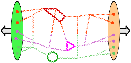
Figure 16: Left: product of a term of the amplitude with a term from the complex conjugate amplitude. Right: interpretation of this product as a cut vacuum graph.

The product of an amplitude by its complex conjugate can be interpreted as performing a cut through a vacuum graph (i.e. a graph without any external gluon)[91, 92]. To construct the generating functional $F[z]$, one simply needs to weight each cut propagator (the propagators with a cross in the right part of the figure 16) by the appropriate function $z({\boldsymbol{p}})$. From this generating functional, the single inclusive gluon spectrum introduced above is given by

$$\frac{dN_{1}}{d^{3}{{\boldsymbol{p}}}}=\left.\frac{\delta F[z]}{\delta z({\boldsymbol{p}})}\right|_{z=1}\;.$$ (78)

In fact, quite generally, inclusive observables are derivatives of $F[z]$ at $z=1$, while exclusive observables are obtained via derivatives at other values of $z$.

A crucial property in the CGC effective theory is unitarity, i.e. at a basic level the fact that the sum of the probabilities for all the possible final states in a collision should equal unity. In terms of the generating functional $F[z]$, unitarity is encoded in a very simple way, $F[1]=1$. The fact that inclusive observables are given by derivatives at $z\equiv 1$, combined to this property due to unitarity, is the reason why they are much simpler than exclusive observables. In more physical terms, inclusive observables are simpler because many graphs cancel thanks to unitarity.

By using reduction formulas for the transition amplitudes and their complex conjugate, one can write the generating functional $F[z]$ as follows

$${{F[z]}=e^{{\cal C}[z]}\left.\;Z[j_{+}]\;Z^{*}[j_{-}]\right|_{j_{+}=j_{-}=j}}\;,$$ (79)

where $Z[j]$ is the usual generating functional for the time-ordered Green’s functions that enter in the reduction formulas[93], and where

$${{\cal C}[z]}\equiv\int d^{4}xd^{4}y\;{G_{+-}^{0}(x,y)}\;\square_{x}\square_{y}\;\frac{\delta}{\delta{j_{+}(x)}}\frac{\delta}{\delta{j_{-}(y)}}$$

$${G_{+-}^{0}(x,y)}\equiv\int\frac{d^{4}p}{(2\pi)^{4}}\;e^{ip\cdot(x-y)}\;{z({\boldsymbol{p}})}\;{2\pi\theta(-p^{0})\delta(p^{2})} \;.$$

(Note that here we have simplified the notations by not writing color, Lorentz and polarization indices – when dealing with gluons, these indices are of course necessary.) Eq. (79), albeit being rather formal, is useful to obtain more explicit expressions for observables than can be derived from the generating functional. At this point, it is crucial to note that

$$e^{{\cal C}[1]}\;Z[j_{+}]\;Z^{*}[j_{-}]={\cal Z}[j_{+},j_{-}]\;,$$ (80)

where ${\cal Z}[j_{+},j_{-}]$ is the generating functional for path-ordered Green’s functions in the Schwinger-Keldysh formalism[94, 95].

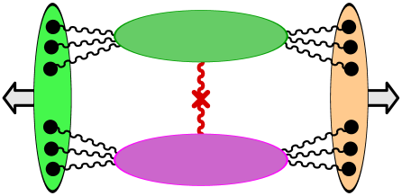
Figure 17: Diagrammatic representation of the two terms in the right hand side of eq. (81). Left: term in $A_{+}A_{-}$. Right: term in $G_{+-}$. The crossed wavy line represents the on-shell momentum ${\boldsymbol{p}}$.

For instance, one can use eq. (79) in order to obtain the following expression for the single inclusive spectrum,

$$\frac{dN_{1}}{d^{3}{\boldsymbol{p}}}=\left.\frac{\delta F[z]}{\delta({\boldsymbol{p}})}\right|_{z=1}=\int d^{4}xd^{4}y\;e^{ip\cdot(x-y)}\;\square_{x}\square_{y}\Big{[}{A_{+}(x)A_{-}(y)}+{G_{+-}(x,y)}\Big{]}\;,$$ (81)

where $A_{\pm}$ and $G_{+-}$ are respectively the one-point and two-point Green’s functions in the Schwinger-Keldysh formalism. The two terms in this formula are illustrated in the figure 17. This formula is true to all orders, and evaluating the spectrum at a given order amounts to evaluated these Green’s functions to the desired order (the power counting rule of eq. (73) can be applied to these functions, respectively with $n_{{}_{E}}=1$ and $n_{{}_{E}}=2$).

4.4 Leading order and retarded classical fields

When we apply the power counting rule (73) to $A_{\pm}$ and $G_{+-}$, we see that they have the following expansion in $g^{2}$

$$A_{\pm} = \frac{a_{0}}{g}+a_{1}\,g+a_{2}\,g^{3}+\cdots$$

$$G_{+-} = b_{0}+b_{1}\,g^{2}+b_{2}\,g^{4}+\cdots\;,$$ (82)

where the $a_{i}$ and $b_{i}$ are coefficients of order one. Therefore, to evaluate the spectrum at leading order, we need only the LO of $A_{\pm}$, and we can disregard completely the term with $G_{+-}$, as illustrated in the left figure 18.

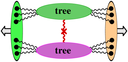
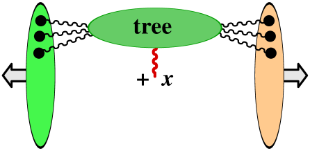
Figure 18: Left: only contribution to the single inclusive spectrum at leading order. Right: $A_{+}(x)$ at leading order.

Despite this simplification, one still needs to sum an infinite set of graphs. Indeed, all the tree topologies contribute to $A_{\pm}$ at the order $1/g$, and for all the internal vertices, we must sum over all the possible assignments of the types $+$ or $-$, per the rules of the Schwinger-Keldysh formalism[94, 95]. Since the color sources are identical on the two branches of the Schwinger-Keldysh closed time contour, this sum only gives the following combinations of propagators

$$G_{++}^{0}(p)-G_{+-}^{0}(p)=G_{-+}^{0}(p)-G_{--}^{0}(p){=G_{{}_{R}}^{0}(p)}\;,$$ (83)

i.e. the retarded propagator. Thus, we only need to sum all the tree diagrams built with retarded propagators, as illustrated in the figure 19.

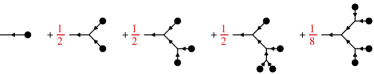
Figure 19: Beginning of the series of tree diagrams that contribute to $A_{\pm}$ at LO (only cubic vertices are included here, but of course in QCD one would also have four-gluon vertices). The black dots denote the color sources $\rho_{1}$ or $\rho_{2}$, and the arrows on the lines indicate that the propagators are retarded.

The result of this sum of tree graphs is well known: it is the solution of the classical field equations of motion that vanishes in the remote past. In the case of QCD, these are the Yang-Mills equations,

$$\left[{\cal D}_{\mu},{\cal F}^{\mu\nu}\right]=\delta^{\nu-}\rho_{1}+\delta^{\nu+}\rho_{2}\quad,\qquad\lim_{x^{0}\to-\infty}{\cal A}^{\mu}(x)=0\;.$$ (84)

This result is what justifies the procedure described in the introduction of this section in order to compute the inclusive gluon spectrum.

Interestingly, at LO, the $n$-gluon inclusive spectrum factorizes into products of single gluon spectra,

$$\left.\frac{d{{{N_{n}}}}}{d^{3}{\boldsymbol{p}}_{1}\cdots d^{3}{\boldsymbol{p}}_{n}}\right|_{{}_{\rm LO}}=\left.\frac{d{{{N_{1}}}}}{d^{3}{\boldsymbol{p}}_{1}}\right|_{{}_{\rm LO}}\times\cdots\times\left.\frac{d{{{N_{1}}}}}{d^{3}{\boldsymbol{p}}_{n}}\right|_{{}_{\rm LO}}\;,$$ (85)

as can be checked by simple power counting arguments.

4.5 Next to Leading Order, logarithms and factorization

The previous discussion justifies partly the procedure employed to compute observables in the CGC framework. But since it is based solely on LO considerations, it says nothing about the logarithmic cutoff dependence that may arise in loop corrections. Indeed, in eq. (74), it is implicitly assumed that the coefficients $c_{0},c_{1},\cdots$ are of order one. But these coefficients in fact contain logarithms of the cutoff, and should be more accurately written as

$$c_{1} = c_{10}\; + {c_{11}\,\ln\Lambda^{\pm}}\;\;\;\;$$

$$c_{2} = c_{20}\; + c_{21}\,\log\Lambda^{\pm}\; + \underbrace{{c_{22}\,\log^{2}\Lambda^{\pm}}}\;\;\;\;$$

Leading Log terms

At each order, there can be powers of logarithms up to the number of loops. The terms that maximize the number of logarithms are called the Leading Log terms, and are the most important.

On a more phenomenological side, the above LO result for the gluon spectrum is insufficient because at this order the spectrum has no dependence on the rapidity of the produced gluon. The two issues are in fact closely related : logarithms of the cutoff appear at NLO, and in order to cancel them one must let the distributions of sources $W_{1}[\rho_{1}]$ and $W_{2}[\rho_{2}]$ evolve according to the JIMWLK equation. It is this evolution that gives the spectrum its rapidity dependence.

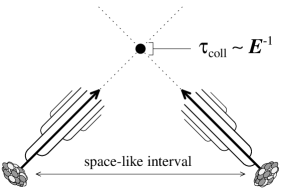
Figure 20: Causality argument explaining why the distributions $W[\rho]$ are universal in nucleus-nucleus collisions.

Let us first start with a qualitative argument to explain why it should be possible to absorb the logarithms of the cutoff into universal distributions $W[\rho]$ in the case of nucleus-nucleus collisions (in fact the same distributions as those encountered in DIS). This argument, based on causality, is illustrated in the figure 20, and goes as follows

• The duration of the collision is very short, and decreases as the inverse of the collision energy.

• In contrast, the radiation of the soft gluons responsible for the logarithms takes a much longer time. Therefore, this radiation cannot happen during the collision itself – these gluons must be emitted before the collision.

• Before the collision, the two nuclei are not in causal contact. Therefore, what happens inside the first nucleus cannot be influenced by the second nucleus, and conversely. It should also be independent of the quantities that an observer may measure in the final state (provided that this measurement does not lead to discarding some class of events – hence the special role of inclusive observables). Therefore, each nucleus should be described by a universal distribution $W[\rho]$.

Figure 21: Left: diagrams in the gluon spectrum at LO. Middle and Right: diagrams in the gluon spectrum at NLO. Here, the graphs are represented in coordinate space (with the two light-cones figuring the trajectories of the colliding nuclei). The green and red dots are the color sources carried by the two nuclei.

Now, let us consider the NLO corrections to the single inclusive gluon spectrum, in order to see more precisely the structure of the logarithms. There are two types of contributions at NLO, represented in the middle and right graphs of the figure 21 (for comparison, we have represented in the left graph a typical contribution at LO). The graph in the middle involves the two-point Green’s function $G_{+-}(x,y)$, that makes a first appearance at NLO, while the graph on the right contains a one-loop correction to the factor $A_{+}(x)$ (there is a third class of graphs, not shown in the figure 21, that contain a one-loop correction to $A_{-}(y)$).

The calculation of the NLO correction to the gluon spectrum is rather involved and will not be detailed here. Instead, we just sketch the main steps in this study[96, 97, 98],

• Express the single gluon spectrum at LO and NLO in terms of classical fields and small field fluctuations. A crucial property is that these objects all obey retarded boundary conditions.

• Write the NLO terms as a perturbation of the initial value of the classical fields. If ${\cal A}^{\mu}(x)$ is a solution of the classical Yang-Mills equations, and $a^{\mu}(x)$ a small (in the sense that $a^{\mu}\ll{\cal A}^{\mu}$, so that the equation of motion of $a^{\mu}$ can be linearized) perturbation around this solution, they are formally related by

  $${{\boldsymbol{a}}^{\mu}(x)}\equiv\int\limits_{{\boldsymbol{u}}\in\Sigma}\big{[}{\alpha}({\boldsymbol{u}})\,{\mathbbm{T}}_{\boldsymbol{u}}\big{]}\;{\cal A}^{\mu}(x)\;,$$ (86)

  where ${\mathbbm{T}}_{\boldsymbol{u}}$ is the generator of the shifts of the initial value of ${\cal A}^{\mu}$ on some surface $\Sigma$ (roughly speaking, one can see ${\mathbbm{T}}_{\boldsymbol{u}}$ as a derivative with respect to the initial value of the field at the point ${\boldsymbol{u}}\in\Sigma$). Thanks to this identity, one can obtain the following formula for the gluon spectrum at NLO

  $$\left.\frac{dN_{1}}{d^{3}{\boldsymbol{p}}}\right|_{{}_{\rm NLO}}=\Big{[}\frac{1}{2}\int\limits_{{}_{{\boldsymbol{u}},{\boldsymbol{v}}\in\Sigma}}{{\cal G}({\boldsymbol{u}},{\boldsymbol{v}})}\,{\mathbbm{T}}_{\boldsymbol{u}}{\mathbbm{T}}_{\boldsymbol{v}}+\int\limits_{{}_{{\boldsymbol{u}}\in\Sigma}}{{\boldsymbol{\beta}}({\boldsymbol{u}})}\,{\mathbbm{T}}_{\boldsymbol{u}}\Big{]}\;\left.\frac{dN_{1}}{d^{3}{\boldsymbol{p}}}\right|_{{}_{\rm LO}}\;,$$ (87)

  where ${\boldsymbol{\beta}}$ and ${\cal G}$ are one-point and two-point functions that can be computed analytically. The main interest of this formula is that it provides a factorization in time of the NLO spectrum: the operator inside the square brackets depends only on the fields under the surface $\Sigma$, while the factor $dN_{1}/d^{3}{\boldsymbol{p}}|_{{}_{\rm LO}}$ on which it acts depends only on what happens above $\Sigma$. Therefore, by choosing appropriately the surface $\Sigma$, this formula separates what happens in the two nuclei before the collision from the collision itself. Note also that in this formula, the first factor can be calculated analytically, while the second cannot because it involves solutions of the classical Yang-Mills equations that are not known analytically.

  

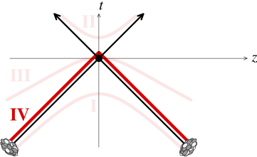
  Figure 22: Choice of the surface $\Sigma$ to extract the initial state logarithms.

• Choose $\Sigma$ as in the figure 22. When ${\boldsymbol{u}},{\boldsymbol{v}}$ are both on the $t=z$ branch of the light-cone, one has :

  $$\frac{1}{2}\int\limits_{{}_{{\boldsymbol{u}},{\boldsymbol{v}}\in\Sigma}}{{\cal G}({\boldsymbol{u}},{\boldsymbol{v}})}\,{\mathbbm{T}}_{\boldsymbol{u}}{\mathbbm{T}}_{\boldsymbol{v}}+\int\limits_{{}_{{\boldsymbol{u}}\Sigma}}{{\boldsymbol{\beta}}({\boldsymbol{u}})}\,{\mathbbm{T}}_{\boldsymbol{u}}=\log{{\Lambda^{+}}}\,\times\,{{\cal H}_{1}}\;+\;\mbox{finite terms}\;,$$ (88)

  where ${\cal H}_{1}$ is the JIMWLK Hamiltonian of the nucleus that moves in the $+z$ direction. If the two points ${\boldsymbol{u}},{\boldsymbol{v}}$ are on the other branch of $\Sigma$, we obtain a logarithm of $\Lambda^{-}$, whose coefficient is the JIMWLK Hamiltonian ${\cal H}_{2}$ of the other nucleus. If the points ${\boldsymbol{u}},{\boldsymbol{v}}$ are on different branches of the light-cone, there is no logarithm. Therefore, at leading log accuracy, we have

  $$\left.\frac{dN_{1}}{d^{3}{\boldsymbol{p}}}\right|_{{}_{\rm NLO}}\;\mathrel{\mathop{\kern 0.0pt=}\limits_{\scriptsize\mbox{Leading Log}}}\;\Big{[}\log\left(\Lambda^{+}\right){{\cal H}_{1}}+\log\left(\Lambda^{-}\right){{\cal H}_{2}}\Big{]}\;\left.\frac{dN_{1}}{d^{3}{\boldsymbol{p}}}\right|_{{}_{\rm LO}}\;.$$ (89)

• Like in the case of DIS, the logarithms can be hidden by integrating over the sources $\rho_{1}$ and $\rho_{2}$, with distributions $W_{1}[\rho_{1}]$ and $W_{2}[\rho_{2}]$ that obey the JIMWLK equation, with the JIMWLK Hamiltonian of the corresponding nucleus. To see this, one simply uses the self-adjointness of the JIMWLK Hamiltonian in order to transpose its action from the observable on the distributions $W[\rho]$. The final formula at Leading Log for the gluon spectrum is

  $$\frac{dN_{1}}{d^{3}{\boldsymbol{p}}}\;\mathrel{\mathop{\kern 0.0pt=}\limits_{\scriptsize\mbox{Leading Log}}}\;\int\big{[}D{\rho_{{}_{1}}}\,D{\rho_{{}_{2}}}\big{]}\;{W_{1}\big{[}\rho_{{}_{1}}\big{]}}\;{W_{2}\big{[}\rho_{{}_{2}}\big{]}}\;\underbrace{\left.\frac{dN_{1}}{d^{3}{\boldsymbol{p}}}\right|_{{}_{\rm LO}}}_{\rm fixed\ \rho_{1,2}}\;.$$ (90)

The factorization formula (90) ends the justification of the procedure employed in the literature in order to evaluate the gluon spectrum in the CGC framework. Similar factorized formulas also exist for $n$-gluon inclusive spectra, or for observables like the energy-momentum tensor. In each of these extensions, it is the same distributions $W[\rho]$ that enter in the formula, therefore providing examples of their universality. In order to extend this factorization to other observables, the central step is to prove that eq. (87) is true for the observable under consideration – with the same operator in the square brackets.

5 Glasma fields, Long range rapidity correlations

5.1 Glasma fields

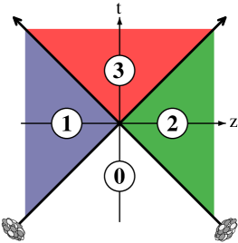
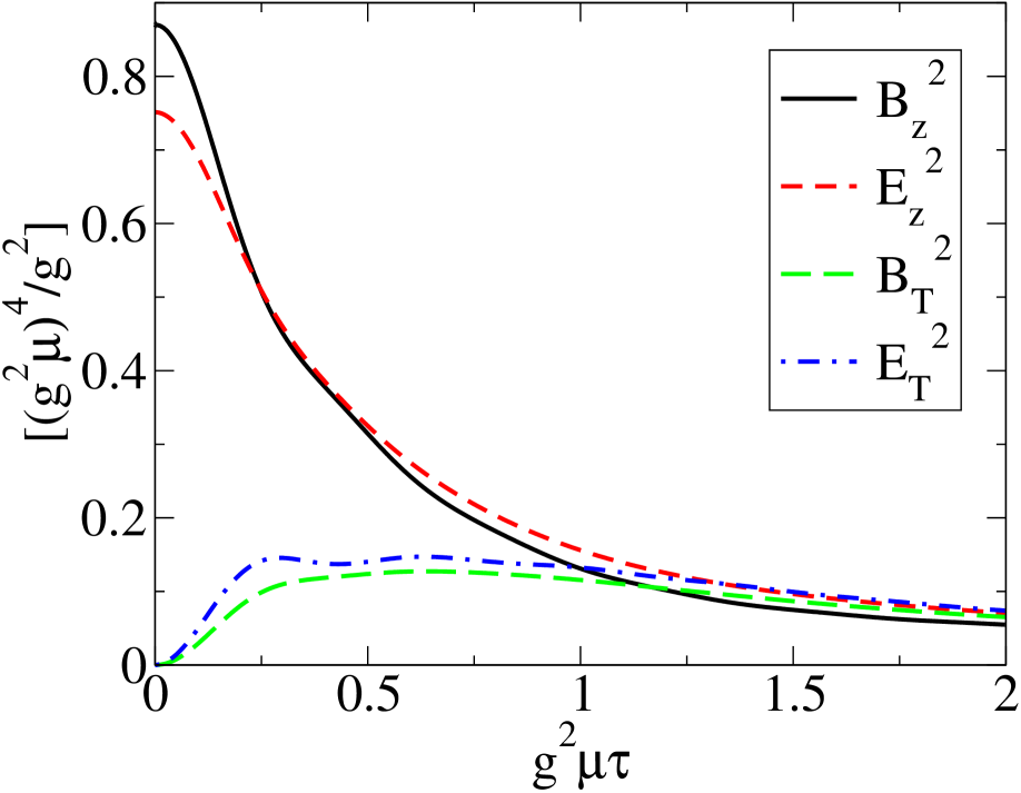
Figure 23: Right: transverse and longitudinal components of the chromo-electric and chromo-magnetic fields in the region three (see the left part of the figure), obtained by solving numerically the classical Yang-Mills equations (72)[99].

The factorization formula (90) indicates that in order to compute the single inclusive spectrum (or any other inclusive quantity, for which the same factorization holds) it is sufficient to compute the gluon spectrum in a classical field obtained by solving the Yang-Mills equation (72), and then to average over all the configurations of the color sources $\rho_{1,2}$. This classical field therefore plays a crucial role in the CGC description of heavy ion collisions, and it is worth spending some time discussing its properties.

First of all, thanks to causality, one can divide space-time in four regions (see the left part of the figure 23). The region labeled zero is completely trivial: an observer in this region sees only the vacuum, and in this region the classical field is zero. Observers in the regions one or two see only one of the nuclei, but not the collision itself. In these regions, the solution of the classical Yang-Mills equations is also very simple. In light-cone gauge, it reads[100],

$${\cal A}^{\pm}=0\quad,\quad{\cal A}^{i}_{1,2}=\frac{i}{g}U_{1,2}^{\dagger}\partial^{i}U_{1,2}\;,$$ (91)

where $U_{1,2}$ is a Wilson line constructed with the source $\rho_{1}$ or $\rho_{2}$ respectively. In the regions one and two, the chromo-electric and chromo-magnetic fields are transverse to the collision axis. Note also that, since these fields are pure gauges, there is no field strength in the regions one and two. In other words, no energy is deposited in these regions.

The most interesting region is the third one, because it causally connected to two nuclei. This region is the locus of all the events that happen after the collision. The gauge fields can be obtained analytically at $\tau=0^{+}$ [101], but one has to resort to numerical methods beyond that. The problem is best formulated in the Fock-Schwinger gauge[102, 101],

$$x^{+}{{\cal A}^{-}}+x^{-}{{\cal A}^{+}}=0\;,$$ (92)

and by exploiting the invariance under longitudinal boosts in collisions at very high energy. If we use the above gauge condition to parameterize the fields ${\cal A}^{\pm}$ as ${\cal A}^{\pm}\equiv\pm x^{\pm}\beta$, then the function $\beta$ and the transverse fields ${\cal A}^{i}$ are independent of the rapidity $\eta$. Solving numerically the Yang-Mills equations in the forward light-cone leads to the chromo-electric and chromo-magnetic fields shown in the right plot of the figure 23. At $\tau=0^{+}$, i.e. just after the collision, these fields have vanishing transverse components: the field lines are all parallel to the collision axis, and form elongated tubular structures. Later on, as time increases, the transverse components of the fields become comparable to the longitudinal components. The glasma designates these strong color fields that populate the system at early times[99].

In the longitudinal direction, the correlation length of the fields is infinite at leading order (since the system is boost invariant). When the leading log corrections are resummed, the distributions of sources evolve with rapidity, thus breaking the boost invariance. However, since the resummed terms are powers of $\alpha_{s}\Delta\eta$, it takes at least a rapidity shift $\Delta\eta\sim\alpha_{s}^{-1}$ in order to see an appreciable variation of the sources. Therefore, even after summing the leading logs, the glasma fields remain coherent over rapidity intervals of order $\alpha_{s}^{-1}$. In the transverse direction, the correlation length of the glasma fields is controlled by the saturation momentum[103], and is therefore of order $Q_{s}^{-1}$.

The fact that the field lines are parallel to the collision axis immediately after the collision leads to a very peculiar form for the energy-momentum tensor,

$$T^{\mu\nu}={\rm diag}\,(\epsilon,\epsilon,\epsilon,{-\epsilon})\;.$$ (93)

The most striking feature is that the longitudinal pressure is negative, which is reminiscent of strings stretching in the longitudinal direction. As we shall see in the section 6, this result is not the end of the story though, and further resummations are necessary due to the presence of instabilities in the solutions of the classical Yang-Mills equations.

5.2 Long range rapidity correlations

The correlation properties of the glasma fields have been proposed as the source of the long range rapidity correlations observed among pairs of hadrons in heavy ion collisions[104, 105, 106, 107, 108, 109, 110, 111].

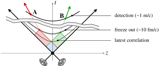
Figure 24: Left: measured two-hadron correlation, as a function of the rapidity difference and azimuthal angle difference between the two hadrons[105]. Right: causal structure of the two-particle correlations.

The data is shown in the left part of the figure 24. It displays several features: a central peak (centered at $\Delta\eta=\Delta\varphi=0$) that can be interpreted as due to collinear fragmentation of a fast particle, and a ridge-like structure, narrow in $\Delta\varphi$ and very elongated in $\Delta\eta$. The rest of the discussion will focus on the latter.

Before trying to interpret this correlation, one can reach a very general conclusion, based on causality, regarding the nature of the phenomena that may produce it. This is illustrated in the right part of the figure 24. Consider two particles A and B, and assume that they are correlated. They are detected long after the collision (compared to the strong interaction timescales), and their last interaction occurred on the freeze-out surface, at a proper time of order $\tau_{f}\approx 10~{}$fm/c. Between their last interaction and their detection, they traveled on straight lines, with an angle determined by their rapidity. From the point at which they crossed the freeze-out surface, draw a light-cone pointing in the past direction: these light-cones (in red and green in the figure) are the locus of the events that may have influenced A or B respectively. Any event outside these light-cones cannot possibly have any influence, by causality. A correlation between A and B means that some event had an influence on both A and B; therefore this event must lie in the overlap of the two light-cones described above, i.e. in the region in blue in the figure. From this figure, we see that this overlap region extends only to a maximal time,

$$\tau_{\rm correlation}\;\leq\;\tau_{f}\;\;e^{-|\Delta y|/2}\;.$$ (94)

This upper bound depends exponentially on the rapidity separation between the two particles, and therefore becomes very small for long range correlations in rapidity. This simple argument tells us that, regardless of their precise nature, the effects that produce these correlations must happen very shortly after the collision, or pre-exist in the wavefunctions of the colliding nuclei.

The leading log factorization formula that generalizes eq. (90) to the two-particle correlation is[97, 98]

$$\frac{dN_{2}}{d^{3}{\boldsymbol{p}}_{1}d^{3}{\boldsymbol{p}}_{2}}\;\mathrel{\mathop{\kern 0.0pt=}\limits_{\scriptsize\mbox{Leading Log}}}\int\big{[}D{\rho_{{}_{1}}}\,D{\rho_{{}_{2}}}\big{]}\;{W_{1}\big{[}\rho_{{}_{1}}\big{]}}\;{W_{2}\big{[}\rho_{{}_{2}}\big{]}}\;\left.\frac{dN_{1}}{d^{3}{\boldsymbol{p}}_{1}}\;\frac{dN_{1}}{d^{3}{\boldsymbol{p}}_{2}}\right|_{{}_{\rm LO}}\;.$$ (95)

Note that the integrand is the product of the single inclusive spectra for gluons of momenta ${\boldsymbol{p}}_{1}$ and ${\boldsymbol{p}}_{2}$ respectively, a consequence of eq. (85). This indicates that, at this order, all the correlations between the two particles result from the averaging over the sources $\rho_{1,2}$, and therefore must come from the distributions $W_{1}[\rho_{1}]$ and $W_{2}[\rho_{2}]$ themselves.

A natural candidate for the formation of long range correlations in rapidity is the glasma color fields[112, 113], since they are coherent over rapidity intervals that extend to at least $\Delta\eta\sim\alpha_{s}^{-1}$ (in turn, the approximate boost invariance of the glasma fields is a consequence of the slow JIMWLK evolution of the distributions $W_{1,2}$, which is an effect of order $\alpha_{s}$). Note that the peculiar structure of the glasma field lines, that form longitudinal tubes at early times, is not essential to this argument. Another important parameter in the argument is the transverse size over which the glasma fields are coherent; this size is of order $Q_{s}^{-1}$. Particles emitted from two distinct glasma flux tubes (i.e. separated by more than $Q_{s}^{-1}$ in the transverse direction) are not correlated (see the left figure 25) since they are produced by incoherent fields.

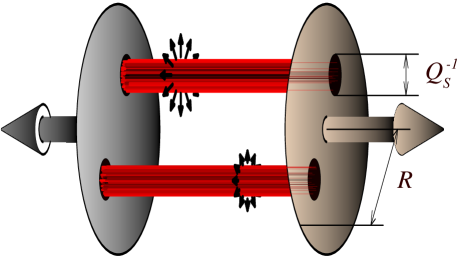
Figure 25: Left: particle emission from two distinct glasma flux tubes. Right: effect of radial flow on the angular distribution of the emitted particles.

The transverse size of the tubes controls the strength of the correlation. Indeed, two particles are correlated only if they come from the same tube. The probability for that is of order $(Q_{s}R)^{-2}$, where $R$ is the typical size of the transverse overlap in the collision (it coincides with the radius of the nuclei in a collision at zero impact parameter).

However, the two-gluon correlation one gets from the glasma fields at early times has no angular dependence: the two particles are not correlated in azimuth. Note that there is no causality argument that tells that the azimuthal correlation must be created early; it can be produced later on by radial flow[114, 115]. The transverse pressure of the matter created in the collision sets it in motion radially, reaching speeds that are a sizable fraction of the speed of light. This collective radial motion transforms an azimuthally flat two-particle spectrum in a spectrum that has a peak around $\Delta\varphi=0$ (see the right figure 24). The width and height of this peak depend on the velocity of the radial flow. In the left plot of the figure 26 is shown a crude calculation of the amplitude of this peak[112] (several works[116, 117] have performed more detailed studies of this effect), based on radial velocities extracted from the data itself[118].

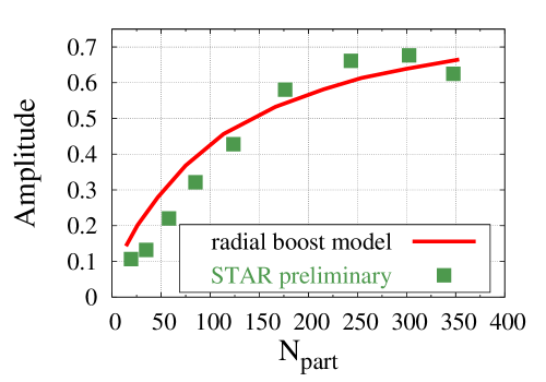
Figure 26: Left: amplitude of the peak in $\Delta\varphi$, compared to data. Right: estimate of the rapidity dependence of the correlation in the CGC (note: the central peak is due to jet fragmentation and has been superimposed by hand) and comparison with data from PHOBOS[119].

From the rapidity dependence of the distributions $W_{1}[\rho_{1}]$ and $W_{2}[\rho 2]$, due to the JIMWLK evolution, it is possible to determine the dependence of the two-gluon spectrum on the rapidities of the two gluons, from eq. (95). Using some shortcuts (such as solving the mean field BK equation, rather than the much more complicated JIMWLK equation), one obtains the rapidity dependence[124] shown in the right plot of the figure 26.

6 Glasma evolution: isotropization and thermalization

6.1 Resummation of the leading secular terms

As we have seen in the previous section, the early stages of heavy ion collisions are dominated by strong color fields, the glasma. Initially, these chromo-electric and chromo-magnetic fields are purely longitudinal. A consequence of this is that the longitudinal pressure is negative (in fact, exactly the opposite of the energy density at $\tau=0^{+}$). This is problematic in view of the many successes of the hydrodynamical description of the evolution of the matter produced in heavy ion collisions[125, 126, 127, 128, 129, 130, 131, 132], because a large and negative pressure poses problems if used as initial condition for hydrodynamics.

However, there is another fact that suggests that the CGC description of nucleus-nucleus collisions that we have described so far is still incomplete. It has been observed in several studies that classical solutions of the Yang-Mills equations suffer from instabilities[133, 134, 135, 136, 137, 138, 139, 140, 141, 142], that make them extremely sensitive to their initial condition.

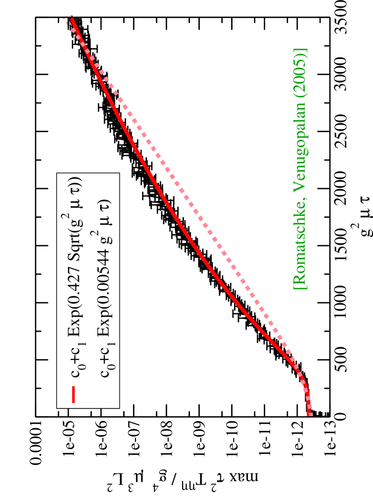
Figure 27: Growth of some instabilities in classical Yang-Mills equations[133].

The plot of the figure 27 shows the growth of such an unstable mode, when one disturbs a boost invariant classical solution by a small rapidity dependent perturbation. These instabilities appear to be related to the well known Weibel instability[143, 144, 145, 146, 147, 148, 149], or filamentation instability, in plasma physics. Many works have already investigated the possible role of these instabilities in the thermalization of the quark-gluon plasma[150, 151, 152, 153, 154, 155, 156, 157, 158, 159, 160, 161, 162, 163].

In the CGC framework, these instabilities question the validity of the power counting that was the very basis for the organization of the expansion in power of $g^{2}$. Indeed, this power counting implicitly assumes that if a classical field ${\cal A}^{\mu}$ is of order $g^{-1}$ and a small perturbation around it is initially of order $1$, then the perturbation remains negligible compared to the background at all times. The existence of instabilities invalidates this assumption. It has been argued that the instabilities grow exponentially as

$$a(\tau)\sim e^{\sqrt{\gamma\tau}}\;,$$ (96)

where the instability growth rate $\gamma$ is of the order of the saturation momentum. This means that it will become comparable in magnitude to the classical background field at a time

$$\tau_{\rm max}\sim\gamma^{-1}\,\log^{2}(g^{-1})\;.$$ (97)

$\tau_{\rm max}$ is the time where the power counting rule in eq. (73) completely breaks down, and the one-loop corrections become as large as the leading order results. These terms, that are formally suppressed by powers of the coupling $g$, but with prefactors that grow with time, are called secular terms.

In order to study the evolution of the system beyond this time, it is necessary to perform a resummation of the secular terms that have the fastest growth in time. A small amendment to the power counting rule of eq. (73) is sufficient to track these terms,

$$\mbox{loop}\sim g^{2}\quad,\qquad{\mathbbm{T}}_{\boldsymbol{u}}\sim e^{\sqrt{\gamma\tau}}\;.$$ (98)

The new rule is to assign a factor $e^{\sqrt{\gamma\tau}}$ to each occurrence of the operator ${\mathbbm{T}}$. The reason for this new rule is eq. (86), that shows that each power of ${\mathbbm{T}}$ generates a perturbation on top of the classical background.

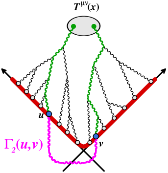
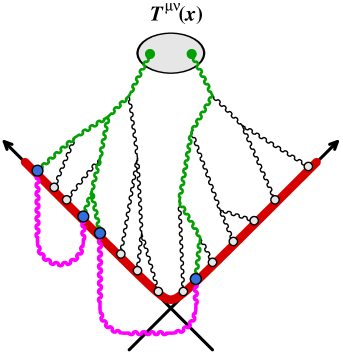
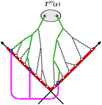
Figure 28: Examples of one-loop and two-loop contributions to the energy momentum tensor. The operators ${\mathbbm{T}}$ are represented as blue dots.

In order to illustrate these rules, we have represented in the figure 28 some one-loop and two-loop contributions to the energy momentum tensor. With these rules, the one-loop graph on the left would bring a factor

$$\big{(}ge^{\sqrt{\gamma\tau}}\big{)}^{2}\;,$$ (99)

and the two-loop graph in the middle a factor

$$\big{(}ge^{\sqrt{\gamma\tau}}\big{)}^{4}\;,$$ (100)

while the two-loop graph on the right gives only

$$g\big{(}ge^{\sqrt{\gamma\tau}}\big{)}^{3}\;.$$ (101)

(These factors are all relative to the tree level result.) At the time $\tau_{\rm max}$, the first two contributions have the same order of magnitude as the leading order result, while the third contribution we have considered in this example is still suppressed. It is easy to resum all the terms that are leading at the time $\tau_{\rm max}$: this corresponds to all the graphs that have the same structure as the first two on the left of the figure 28, with an arbitrary number of loops provided that these loops are not nested below the light-cone. The sum of these graphs can be obtained by exponentiating the operator in the square brackets in eq. (87). For a generic inclusive observable, this reads

$${\cal O}_{\rm resum}=\exp\Big{[}\frac{1}{2}\int\limits_{{}_{{\boldsymbol{u}},{\boldsymbol{v}}\in\Sigma}}{{\cal G}({\boldsymbol{u}},{\boldsymbol{v}})}\,{\mathbbm{T}}_{\boldsymbol{u}}{\mathbbm{T}}_{\boldsymbol{v}}+\int\limits_{{}_{{\boldsymbol{u}}\in\Sigma}}{{\boldsymbol{\beta}}({\boldsymbol{u}})}\,{\mathbbm{T}}_{\boldsymbol{u}}\Big{]}\;{\cal O}_{{}_{\rm LO}}\;,$$ (102)

By construction, this resummation contains the full LO and NLO results, and a subset of all the higher order terms,

$${\cal O}_{\rm resum}=\underbrace{{\cal O}_{{}_{\rm LO}}+{\cal O}_{{}_{\rm NLO}}}_{\scriptsize\mbox{in full}}+\underbrace{{\cal O}_{{}_{\rm NNLO}}+\cdots}_{\scriptsize\mbox{partially}}$$ (103)

Eq. (102) can be turned in a much more practical expression. By noticing that the exponential of ${\mathbbm{T}}$ is a translation operator,

$${\cal F}[{{\cal A}_{\rm initial}}+{\alpha}]\equiv\exp\Bigg{[}\int_{{}_{{\boldsymbol{u}}\in{\Sigma}}}\big{[}{\alpha}\cdot{\mathbbm{T}}\big{]}_{\boldsymbol{u}}\Bigg{]}\;\;{\cal F}[{{\cal A}_{\rm initial}}]\;,$$ (104)

one can rewrite eq. (102) as

$${\cal O}_{\rm resum}=\int[D{\chi}]\,\exp\Bigg{[}-\frac{1}{2}\int\limits_{{}_{{\boldsymbol{u}},{\boldsymbol{v}}}\in\Sigma}{\chi({\boldsymbol{u}})}\;{{\cal G}^{-1}({\boldsymbol{u}},{\boldsymbol{v}})}\;{\chi({\boldsymbol{v}})}\Bigg{]}\;{\cal O}_{{}_{\rm LO}}[{\cal A}_{\rm init}+{\chi}+{\boldsymbol{\beta}}]\;.$$ (105)

In words, the resummed observable is obtained by shifting the initial value on $\Sigma$ (in practice a surface of constant proper time $\tau_{0}$) by a constant shift ${\boldsymbol{\beta}}$ and by a fluctuating shift $\chi$ that has a Gaussian distribution. The variance of this Gaussian distribution can be calculated easily, and the functional integration over $\chi$ in eq. (105) can be evaluated by a Monte-Carlo sampling. This resummation is sometimes described in the literature as classical statistical field theory. The same Gaussian average was also obtained in different approaches[164, 165, 166, 167, 168]. A similar method has also been applied to cold atom physics, in problems related to Bose-Einstein condensation[169, 170].

In the rest of this section, we will present some numerical results illustrating the effect of this resummation. Because its implementation has not yet been completed for Yang-Mills theory[171], we have tried it on a much simpler model[172, 173, 174] –a real scalar field with a $\phi^{4}$ coupling–, that shares with QCD some important features:

• Scale invariance at the classical level in $3+1$ dimensions.

• Instabilities in the classical equations of motion, due to parametric resonance.

Many aspects of this resummation can be studied by considering a system confined in a fixed volume, while other questions require to consider a system that expands longitudinally, as in a high energy collision.

6.2 Evolution of a fixed volume system

Consider first a system in a fixed volume. It is initialized with a large background field that mimics the glasma field of heavy ion collisions, to which we superimpose Gaussian fluctuations given by eq. (105). Then, each field configuration evolves according to the classical equation of motion, and observables are evaluated in its solution. A Monte-Carlo sampling is performed in order to average over the Gaussian ensemble of fluctuations.

Firstly, it is interesting to look at observables in a fixed loop order expansion, in order to highlight the pathologies caused by the presence of instabilities in the theory. This is illustrated in the figure 29, where we show the tree level (left) and one-loop (right) results for the energy density and the pressure.

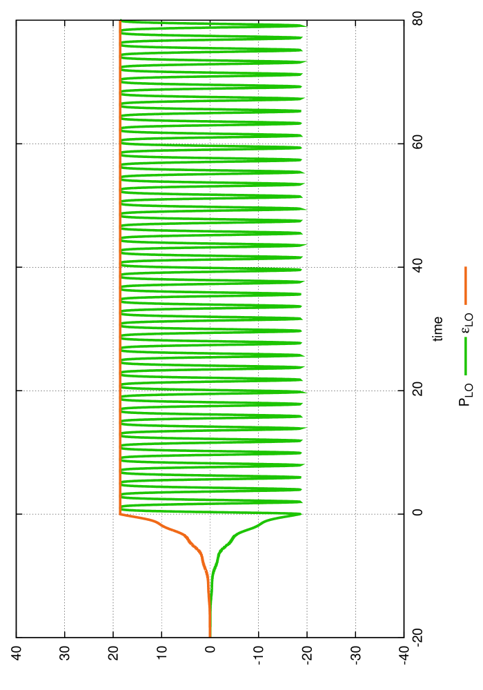
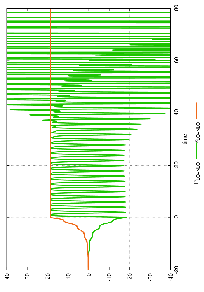
Figure 29: Energy density and pressure in $\phi^{4}$ scalar theory. Left: tree level result. Right: tree level + one-loop result.

(The evolution really starts at $t=0$. At $t<0$, the system is initialized by a source that drives the background field to a large non-zero value.) One sees that the pressure oscillates in time – this means that there is no equation of state, since that would require a one-to-one correspondence between the pressure and the energy density. Even more problematic is the fact that at NLO, the oscillations of the pressure grow exponentially in time, making the predictions of the expansion in $g^{2}$ completely unreliable after a finite time.

In contrast, the resummed pressure behaves in a very different way, as shown in the figure 30.

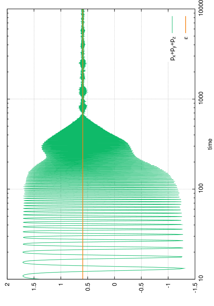
Figure 30:

The oscillations are damped, so that the pressure reaches a fixed value after a certain time. This asymptotic value of the pressure is related to the energy density by a very simple equation of state,

$$\epsilon=3P\;,$$ (106)

which is the expected relationship in a scale invariant theory in 3+1 dimensions. On similar timescales, the spectrum of excitations in the system also becomes considerably simpler, as shown by the spectral functions at two different times in the figure 31.

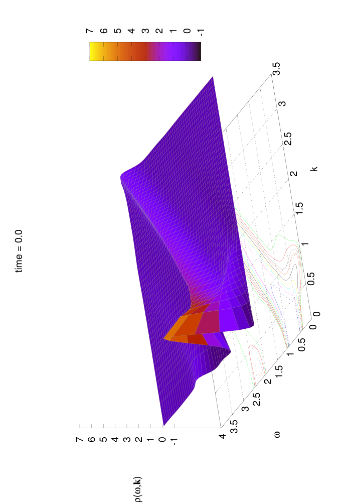
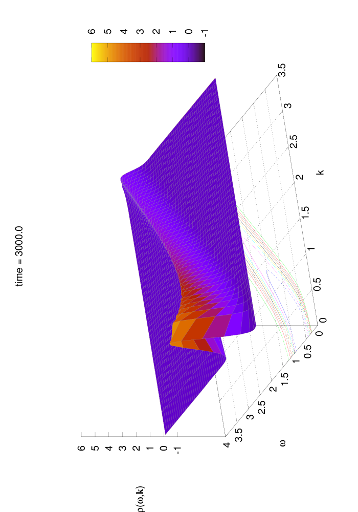
Figure 31: Spectral function of the system at two different times. Left: t=0. Right: t=3000 (in lattice units).

At the initial time, the spectral function has a complicated structure with more than one branch (including a branch that has a negative slope). At later times (comparable to the relaxation time of the pressure), only one branch remains in the spectral function, suggesting that the system can be interpreted as a simple gas of quasiparticles.

However, the relaxation of the pressure does not imply that the system has fully thermalized, as illustrated in the figure 32.

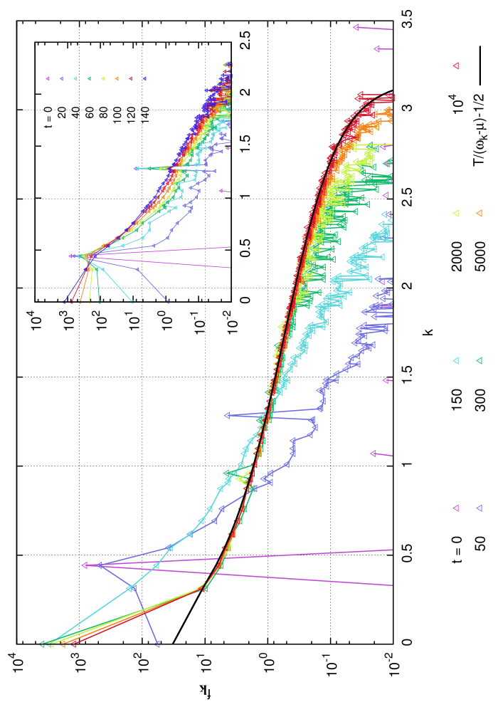
Figure 32: Left: occupation number as a function of momentum at various times. Right: time evolution of the occupation in the zero mode, for various values of the coupling constant.

Here, the background field is chosen such that only a nonzero momentum mode has a large occupation number at the initial time, while all the other modes are empty. Very quickly, particles are produced in all the other modes, including the zero mode, mostly by elastic scatterings. At late times, one can fit the occupation number by a function of the form,

$$F({\boldsymbol{k}})=\frac{T}{\omega_{\boldsymbol{k}}-\mu}-\frac{1}{2}\;,$$ (107)

where $\omega_{\boldsymbol{k}}^{2}={\boldsymbol{k}}^{2}+m^{2}$ with $m$ the quasiparticle mass obtained by studying the spectral function. $T$ and $\mu$ are fitted to the numerical results. This functional form corresponds to the first two terms of the expansion of a Bose-Einstein distribution in the soft sector. Interestingly, the best fit requires a nonzero chemical potential. Since the theory under consideration has no conserved particle number, this suggests that the system is not yet in chemical equilibrium even at the largest times considered. This is expected for the $\phi^{4}$ theory at weak coupling, because the inelastic cross-section (that can equilibrate the particle number) is much smaller than the elastic one.

Another interesting feature is the fact that the fitted value of the chemical potential is very close to the mass of the quasiparticles. This, combined with the fact that there seem to be an excess of particles in the zero mode, suggests that the system undergoes Bose-Einstein condensation. We have confirmed this by showing that the occupation number in the zero mode is proportional to the volume of the system. Of course, in a theory where the particle number is not conserved, a Bose-Einstein condensate cannot be stable. Eventually, the inelastic collisions will eliminate the excess of particles that led to its formation, and dissolve the condensate. This is visible in the right plot of the figure 32, where the occupation number in the zero mode is shown as a function of time. After a very rapid growth, $f(0)$ remains almost constant for a rather long time, to eventually decrease on even longer timescales (the timescales over which the inelastic processes become effective). As expected, by increasing the coupling, the condensate dissolves faster, because the inelastic collision rate is larger.

Whether a Bose-Einstein condensate of gluons can form in heavy ion collisions is still an open question. The condition of overpopulation is initially also satisfied by the glasma fields[179], but the inelastic rates are not parametrically suppressed compared to the elastic ones. Therefore it may happen that the condensate dissolves as fast as it forms, never really becoming a relevant feature of the time evolution.

6.3 Evolution of a longitudinally expanding system

In nucleus-nucleus collisions at high energy, another important question arises: is the longitudinal pressure comparable to the transverse pressure? This is an important aspect in the applicability of hydrodynamics: if the two pressures are two different, then the viscous corrections are large. When discussing the glasma fields, we have seen that at leading order, the longitudinal pressure is in fact the opposite of the energy density at $\tau=0^{+}$. This is in fact a generic feature in any system of longitudinally expanding fields. Indeed, energy and momentum conservation lead to the following equation (for a system homogeneous in the transverse plane)

$$\frac{\partial\epsilon}{\partial\tau}+\frac{\epsilon+P_{{}_{L}}}{\tau}=0\;.$$ (108)

In order to a get a finite $\epsilon$ at $\tau=0^{+}$, it is necessary that $\epsilon+P_{{}_{L}}$ vanishes at $\tau=0^{+}$. As we have seen earlier, this is true in the glasma. This is also the case in the toy scalar model that we have considered in these numerical studies.

A central question is whether the Gaussian fluctuations that are superimposed to the background field can cause the longitudinal pressure to become equal to the transverse one. This question can be addressed in the scalar $\phi^{4}$ model considered in this section. We simply need to use $\tau,\eta$ coordinates, and to setup a boost invariant background field, i.e. independent of $\eta$.

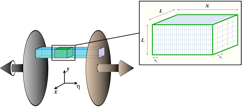
Figure 33: Setup for the lattice study of a system in longitudinal expansion, as in a high energy collision.

The connection between this kind of lattice simulation and an actual collision is illustrated in the figure 33. It would be too costly to simulate the entire volume of the matter produced in a collision, therefore the lattice describes only a small patch of this matter that has a fixed extent in $\eta$ and ${\boldsymbol{x}}_{\perp}$ (and therefore stretches in $z$ as time increases).

The behavior of the energy density, and of the transverse and longitudinal pressures, is shown in the plot on the left of the figure 34. At very early times, the trace of the pressure tensor ($2P_{{}_{T}}+P_{{}_{L}}$) has oscillations. These oscillations are quickly damped, and the system then obeys the equilibrium equation of state,

$$\epsilon=2P_{{}_{T}}+P_{{}_{L}}\;.$$ (109)

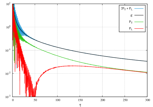
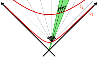
Figure 34: Left: time evolution of the energy density, and of the transverse and longitudinal pressures, in a longitudinal expanding system of scalar fields. Right: illustration of the redshifting of the longitudinal momenta due to longitudinal expansion. The black arrows represent the momentum vectors of particles, and the thin lines their trajectories if they move freely.

However, at this stage of the time evolution, the transverse and longitudinal pressures still behave very differently. The longitudinal pressure decreases much faster, and even becomes negligible compared to the transverse pressure. This is explained naturally by the redshifting of the longitudinal momenta in an expanding system. This effect is illustrated in the right part of the figure 34: if one starts with a broad distribution of longitudinal momenta in a given slice of rapidity $\eta$, after some period of free streaming only the particles that have a momentum rapidity $y$ equal to the space-time rapidity $\eta$ remain in this slice. Thus, the longitudinal pressure (defined in the local rest frame of the matter, i.e. in a frame comoving along the rapidity slice) decreases rapidly.

However, at some point, the longitudinal pressure stops decreasing. Instead, it increases exponentially and becomes very close to the transverse pressure, leading to an almost perfectly isotropic pressure tensor. This radical change of behavior of the longitudinal pressure seems related to the instabilities present in the system: at early times, the expansion rate (proportional to $\tau^{-1}$) of the system is too large for the instabilities to be able to compete efficiently against the redshifting. It is only at later times, when the expansion rate has become low enough, that the instabilities become the driving force in the system.

It is interesting to compare these results, obtained in classical statistical field theory, with hydrodynamical evolution. Naturally, since the transverse and longitudinal pressures are not equal, viscous corrections must be included in the hydrodynamical description to account for this difference.

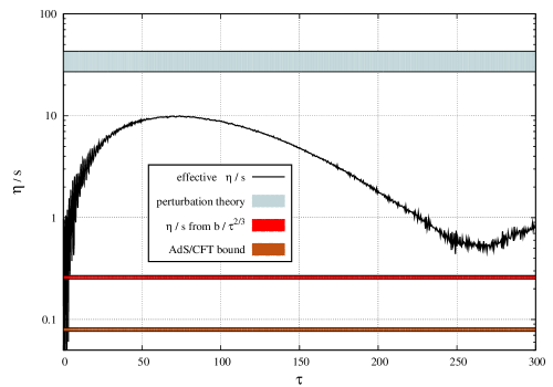
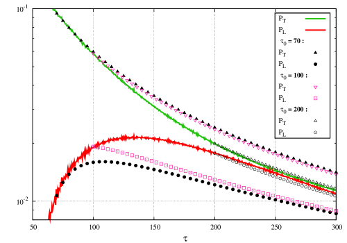
Figure 35: Left: estimate of the viscosity to entropy density ratio. Right: comparison between classical statistical field theory and first order hydrodynamics, for various hydro initial times.

In a system which is homogeneous in the transverse plane and boost invariant, the simplest ansatz is to write

$$P_{{}_{T}}=\frac{\epsilon}{3}+\frac{2\eta}{3\tau}\quad,\quad P_{{}_{L}}=\frac{\epsilon}{3}-\frac{4\eta}{3\tau}\;,$$ (110)

where $\eta$ is the shear viscosity of the system (this corresponds to first order hydrodynamics). In an equilibrated scale invariant fluid, $\eta$ is proportional to the entropy density $s$, and it is customary to quantify how viscous a fluid is by the dimensionless ratio $\eta/s$. If we assume Stefan-Boltzmann’s law for the entropy density, we have $s\approx\epsilon^{3/4}$, and since we know $\epsilon,P_{{}_{T,L}}$ as a function of $\tau$, we can extract from our results an effective value of $\eta/s$. The result of this estimate is shown in the plot on the left of the figure 35. Clearly, the ratio $\eta/s$ is not constant. Its time dependence could be attributed to several causes: first order hydrodynamics (i.e. eq. (110)) may not be a valid description of the system at these early times, and/or the system may still be too far from local equilibrium. Nevertheless, this estimate is instructive because it leads to an $\eta/s$ ratio which is much smaller than the perturbative estimate (blue band in the plot). This may be a manifestation of the anomalously small viscosity that has been conjectured[180, 181] for systems subject to instabilities and turbulence. Note also that the ratio we have extracted remains significantly above the value $1/4\pi$, obtained for certain gauge theories in the limit of infinite coupling.

Another way to compare our results with first order hydrodynamics is to solve eq. (108) with the ansatz of eq. (110) for the longitudinal pressure, under the assumption that the ratio $\eta/s$ is a constant. To close the equation, we may assume again $s\approx\epsilon^{3/4}$. A starting time $\tau_{0}$ must be chosen for this comparison, and the difference between $P_{{}_{T}}$ and $P_{{}_{L}}$ at this initial time determines the value of $\eta/s$. For $\tau>\tau_{0}$, the evolution of the system is governed by eq. (108). This comparison is shown in the plot on the right of the figure 35, for several initial times. It appears that the relaxation $P_{{}_{L}}\to P_{{}_{T}}$ is much faster in the glasma description than in hydrodynamics, presumably due to the effect of instabilities. It is only if the hydrodynamical evolution is started when the system is already well isotropized that it provides a good description of the evolution of the system. Naturally, eq. (108) is certainly valid because it is just a consequence of energy and momentum conservation. Therefore, this comparison questions the validity of the first order approximation to describe the viscous corrections (and the non-constancy of the ratio $\eta/s$ when extracted directly from $P_{{}_{T}}-P_{{}_{L}}$ points also in the same direction). The other conclusion one can make from this comparison, given the fact that hydrodynamics is the limit of kinetic theory when the mean free path goes to zero, is that instabilities are more efficient than collisions to isotropize the system.

7 Conclusions

In this review, we have presented the Color Glass Condensate effective theory, that describes the partonic content of a hadron or nucleus in the saturated regime. Gluon saturation, that happens at high energy, is characterized by large gluon occupation numbers, and by non-linear effects not present in the dilute regime. In order to describe collisions involving hadrons in this regime, one needs a framework that provides a handle on multi-gluon Fock states in the hadron wavefunction, and the tools to perform calculations with these states.

The Color Glass Condensate approximates the fast partons as stochastic classical color sources, while the usual field description is retained for the slow gluons. The requirement that observables be independent on the cutoff that separates these two types of degrees of freedom leads to a renormalization group equation (the JIMWLK equation) for the distribution of the classical sources.

A crucial aspect of the physics of gluon saturation is that the non-linear dynamics generates a semi-hard scale, the saturation momentum. This scale, that increases with energy, plays a crucial role because it sets the value of the strong coupling constant, allowing a weak coupling treatment of gluon saturation. Nevertheless, even at weak coupling, the study of hadronic or nuclear collisions in the saturated regime is non-perturbative, because the smallness of the coupling is compensated by the large occupation numbers for the gluons below the saturation momentum.

The Color Glass Condensate framework proves especially useful in the study of heavy ion collisions at high energy, because the bulk of particle production in these collisions is controlled by the physics of gluon saturation. Moreover, it has been shown that inclusive observables can be factorized (at leading logarithmic accuracy so far) as a convolution of universal distributions of color sources representing the gluon content of the two colliding nuclei, and an observable evaluated in the retarded classical field produced by these sources.

The universality of these distributions of sources, and therefore of the classical color field they produce, confers to these field configurations –the glasma– a very central role in the CGC description of heavy ion collisions. At very short times after the collision, they are characterized by longitudinal chromo-electric and chromo-magnetic fields that are nearly boost invariant, with a transverse correlation length of the order of the inverse saturation momentum. In particular, these fields that have long range correlations in rapidity have been invoked in order to explain the observed two-hadron correlations in heavy ion collisions.

The initial glasma fields form a system which is very from local equilibrium: it is a coherent state rather than a mixed thermal state, and it has a large negative longitudinal pressure. Moreover, these fields are unstable against small perturbations of their initial conditions. In fixed order CGC calculations, these unstable modes lead to secular divergences in quantities such as the energy-momentum tensor. This pathology can be cured by a resummation that amounts to letting the initial glasma field fluctuate around its classical value, with a Gaussian spectrum determined by a one-loop calculation. A numerical implementation of this resummation in a much simpler scalar field theory has recently shown that the instabilities lead to the isotropization of the transverse and longitudinal pressures shortly after the collision, and to full thermalization on longer timescales. Whether this is also the case in QCD, and over which timescale, is the subject of ongoing works.

References

- [1] F. Karsch, et al. [RBC and HotQCD Collaboration], J. Phys. G35, 104096 (2008).
- [2] F.D. Aaron, et al, [H1 and ZEUS Collaborations] JHEP 1001, 109 (2010).
- [3] L.V. Gribov, E.M. Levin, M.G. Ryskin, Phys. Rept. 100, 1 (1983).
- [4] A.H. Mueller, J-W. Qiu, Nucl. Phys. B 268, 427 (1986).
- [5] J.P. Blaizot, A.H. Mueller, Nucl. Phys. B 289, 847 (1987).
- [6] E. Iancu, D.T. Triantafyllopoulos, Nucl. Phys. A 756, 419 (2005).
- [7] E. Iancu, D.T. Triantafyllopoulos, Phys. Lett. B 610, 253 (2005).
- [8] A.H. Mueller, A.I. Shoshi, S.M.H. Wong, Nucl. Phys. B 715, 440 (2005).
- [9] A. Kovner, M. Lublinsky, Phys. Rev. D 71, 085004 (2005).
- [10] A. Kovner, M. Lublinsky, Phys. Rev. Lett. 94, 181603 (2005).
- [11] Y. Hatta, E. Iancu, L. McLerran, A. Stasto, D.N. Triantafyllopoulos, Nucl.Phys. A 764, 423 (2006).
- [12] I. Balitsky, Phys. Rev. D 72, 074027 (2005).
- [13] E. Iancu, R. Venugopalan, Quark Gluon Plasma 3, Eds. R.C. Hwa and X.N. Wang, World Scientific, hep-ph/0303204.
- [14] T. Lappi, Int. J. Mod. Phys. E20, 1 (2011).
- [15] H. Weigert, Prog. Part. Nucl. Phys. 55, 461 (2005).
- [16] F. Gelis, E. Iancu, J. Jalilian-Marian, R. Venugopalan, Ann. Rev. Part. Nucl. Sci. 60, 463 (2010).
- [17] E.A. Kuraev, L.N. Lipatov, V.S. Fadin, Sov. Phys. JETP 45, 199 (1977).
- [18] I. Balitsky, L.N. Lipatov, Sov. J. Nucl. Phys. 28, 822 (1978).
- [19] Yu.V. Kovchegov, Phys. Rev. D 60, 034008 (1999).
- [20] Yu.V. Kovchegov, Phys. Rev. D 61, 074018 (2000).
- [21] A. Deshpande, R. Ent, R. Milner, CERN Courier, October 2009.
- [22] I. Balitsky, Phys. Rev. D 75, 014001 (2007).
- [23] I. Balitsky, G.A. Chirilli, Phys. Rev. D 77, 014019 (2008).
- [24] Yu.V. Kovchegov, H. Weigert, Nucl. Phys. A 784, 188 (2007).
- [25] E. Gardi, J. Kuokkanen, K. Rummukainen, H. Weigert, Nucl. Phys. A 784, 282 (2007).
- [26] J.L. Albacete, N. Armesto, J.G. Milhano, C.A. Salgado, U.A. Wiedemann, Phys. Rev. D 71, 014003 (2005).
- [27] J.L. Albacete, Y. Kovchegov, Phys. Rev. D 75, 125021 (2007).
- [28] J.L. Albacete, N. Armesto, J.G. Milhano, C.A. Salgado, Phys. Rev. D 80, 034031 (2009).
- [29] J.L. Albacete, N. Armesto, J.G. Milhano, C.A. Salgado, arXiv:0906.2721.
- [30] I. Balitsky, Nucl. Phys. B 463, 99 (1996).
- [31] S. Munier, R. Peschanski, Phys. Rev. Lett. 91, 232001 (2003).
- [32] S. Munier, R. Peschanski, Phys. Rev. D 69, 034008 (2004).
- [33] S. Munier, R. Peschanski, Phys. Rev. D 70, 077503 (2004).
- [34] A.M. Stasto, K. Golec-Biernat, J. Kwiecinski, Phys. Rev. Lett. 86, 596 (2001).
- [35] F. Gelis, R. Peschanski, L. Schoeffel, G. Soyez, Phys. Lett. B.647, 376 (2007).
- [36] A. Freund, K. Rummukainen, H. Weigert, A. Schafer, Phys. Rev. Lett. 90, 222002 (2003).
- [37] H. Kowalski, D. Teaney, Phys. Rev. D 68, 114005 (2003).
- [38] H. Kowalski, T. Lappi, R. Venugopalan, Phys. Rev. Lett. 100, 022303 (2008).
- [39] Yu.V. Kovchegov, K. Tuchin, Phys. Rev. D 65, 074026 (2002).
- [40] C. Marquet, B.-W. Xiao, F. Yuan, Phys. Lett. B 682, 207 (2009).
- [41] Yu.V. Kovchegov, K. Tuchin, hep-ph/0603055.
- [42] A. Dumitru, J. Jalilian-Marian, Phys. Rev. Lett. 89, 022301 (2002).
- [43] A. Dumitru, J. Jalilian-Marian, Phys. Lett. B 547, 15 (2002).
- [44] F. Gelis, J. Jalilian-Marian, Phys. Rev. D 66, 014021 (2002).
- [45] F. Gelis, J. Jalilian-Marian, Phys. Rev. D 66, 094014, (2002).
- [46] F. Gelis, J. Jalilian-Marian, Phys. Rev. D 67, 074019 (2003).
- [47] F. Gelis, J. Jalilian-Marian, Phys. Rev. D 76, 074015 (2007).
- [48] A. Dumitru, L.D. McLerran, Nucl. Phys. A 700, 492 (2002).
- [49] J.P. Blaizot, F. Gelis, R. Venugopalan, Nucl. Phys. A 743, 13 (2004).
- [50] J.P. Blaizot, F. Gelis, R. Venugopalan, Nucl. Phys. A 743, 57 (2004).
- [51] E. Iancu, K. Itakura, D. Triantafyllopoulos, Nucl. Phys. A 742, 182 (2004).
- [52] J. Jalilian-Marian, Nucl. Phys. A 748, 664 (2005).
- [53] J. Jalilian-Marian, Nucl. Phys. A 748, 664 (2005).
- [54] J. Jalilian-Marian, Nucl. Phys. A 753, 307 (2005).
- [55] J. Jalilian-Marian, Nucl. Phys. A 770, 210 (2006).
- [56] J. Jalilian-Marian, Y. Kovchegov, Prog. Part. Nucl. Phys. 56, 104 (2006).
- [57] J. Jalilian-Marian, Y. Kovchegov, Phys. Rev. D 70, 114017 (2004), Erratum-ibid. D 71, 079901 (2005).
- [58] H. Fujii, F. Gelis, R. Venugopalan, Phys. Rev. Lett. 95, 162002 (2005).
- [59] A. Dumitru, A. Hayashigaki, J. Jalilian-Marian, Nucl. Phys. A 765, 464 (2006).
- [60] A. Dumitru, A. Hayashigaki, J. Jalilian-Marian, Nucl. Phys. A 770, 57 (2006).
- [61] A. Dumitru, J. Jalilian-Marian, Phys. Rev. D 81, 094015 (2010).
- [62] C. Marquet, Nucl. Phys. A 796, 41 (2007).
- [63] F. Dominguez, B.W. Xiao, F. Yuan, arXiv:1009.2141.
- [64] G.A. Chirilli, B.-W. Xiao, F. Yuan, Phys. Rev. D 86, 054005 (2012).
- [65] L.D. McLerran, R. Venugopalan, Phys. Rev. D 49, 2233 (1994).
- [66] L.D. McLerran, R. Venugopalan, Phys. Rev. D 49, 3352 (1994).
- [67] L.D. McLerran, R. Venugopalan, Phys. Rev. D 50, 2225 (1994).
- [68] A. Ayala, J. Jalilian-Marian, L.D. McLerran, R. Venugopalan, Phys. Rev. D 53, 458 (1996).
- [69] J. Jalilian-Marian, A. Kovner, L.D. McLerran, H. Weigert, Phys. Rev. D 55, 5414 (1997).
- [70] J. Jalilian-Marian, A. Kovner, A. Leonidov, H. Weigert, Nucl. Phys. B 504, 415 (1997).
- [71] J. Jalilian-Marian, A. Kovner, A. Leonidov, H. Weigert, Phys. Rev. D 59, 014014 (1998).
- [72] J. Jalilian-Marian, A. Kovner, A. Leonidov, H. Weigert, Phys. Rev. D 59, 034007 (1999).
- [73] J. Jalilian-Marian, A. Kovner, A. Leonidov, H. Weigert, Phys. Rev. D 59, 099903 (1999).
- [74] E. Iancu, A. Leonidov, L.D. McLerran, Nucl. Phys. A 692, 583 (2001).
- [75] E. Iancu, A. Leonidov, L.D. McLerran, Phys. Lett. B 510, 133 (2001).
- [76] E. Ferreiro, E. Iancu, A. Leonidov, L.D. McLerran, Nucl. Phys. A 703, 489 (2002).
- [77] L.D. McLerran, R. Venugopalan, Phys. Rev. D 59, 094002 (1999).
- [78] L.D. McLerran, R. Venugopalan, Phys. Lett. B 424, 15 (1998).
- [79] A. Krasnitz, R. Venugopalan, Nucl. Phys. B 557, 237 (1999).
- [80] A. Krasnitz, R. Venugopalan, Phys. Rev. Lett. 84, 4309 (2000).
- [81] A. Krasnitz, R. Venugopalan, Phys. Rev. Lett. 86, 1717 (2001).
- [82] A. Krasnitz, Y. Nara, R. Venugopalan, Phys. Rev. Lett. 87, 192302 (2001).
- [83] A. Krasnitz, Y. Nara, R. Venugopalan, Nucl. Phys. A 727, 427 (2003).
- [84] T. Lappi, Phys. Rev. C 67, 054903 (2003).
- [85] T. Lappi, Phys. Lett. B 643, 11 (2006).
- [86] A. Krasnitz, Y. Nara, R. Venugopalan, Phys. Lett. B 554, 21 (2003).
- [87] A. Krasnitz, Y. Nara, R. Venugopalan, Nucl. Phys. A 717, 268 (2003).
- [88] T. Lappi, R. Venugopalan, Phys. Rev. C 74, 054905 (2006).
- [89] F. Gelis, R. Venugopalan, Nucl. Phys. A 776, 135 (2006).
- [90] F. Gelis, R. Venugopalan, Nucl. Phys. A 779, 177 (2006).
- [91] R.E. Cutkosky, J. Math. Phys. 1, 429 (1960).
- [92] G. t’Hooft, M.J.G. Veltman, CERN report 73-9.
- [93] C. Itzykson, J.B. Zuber, Quantum field theory, McGraw-Hill (1980).
- [94] J. Schwinger, J. Math. Phys. 2, 407 (1961).
- [95] L.V. Keldysh, Sov. Phys. JETP 20, 1018 (1964).
- [96] F. Gelis, T. Lappi, R. Venugopalan, Phys. Rev. D 78, 054019 (2008).
- [97] F. Gelis, T. Lappi, R. Venugopalan, Phys. Rev. D 78, 054020 (2008).
- [98] F. Gelis, T. Lappi, R. Venugopalan, Phys. Rev. D 79, 094017 (2009).
- [99] T. Lappi, L.D. McLerran, Nucl. Phys. A 772, 200 (2006).
- [100] Yu.V. Kovchegov, Phys. Rev. D 54, 5463 (1996).
- [101] A. Kovner, L.D. McLerran, H. Weigert, Phys. Rev. D 52, 6231 (1995).
- [102] A. Kovner, L.D. McLerran, H. Weigert, Phys. Rev. D 52, 3809 (1995).
- [103] E. Iancu, K. Itakura, L.D. McLerran, Nucl. Phys. A 724, 181 (2003).
- [104] M. Daugherity, [STAR Collaboration] PoS C FRNC2006, 005 (2006).
- [105] B.I. Abelev, et al., [STAR Collaboration] Phys. Rev. C 80, 064912 (2009).
- [106] J. Adams, et al., [STAR Collaboration] Phys. Rev. Lett. 95, 152301 (2005).
- [107] J. Adams, et al., [STAR Collaboration] Phys. Rev. C 73, 064907 (2006).
- [108] F. Wang, [STAR Collaboration] talk at Quark Matter 2004, J. Phys. G 30, S1299 (2004).
- [109] A. Adare, et al., [PHENIX Collaboration] Phys. Rev. C 78, 014901 (2008).
- [110] B. Wosiek, [PHOBOS Collaboration], Quark Matter 2008, J. Phys. G35, 104005 (2008).
- [111] [CMS Collaboration], JHEP 1009, 091 (2010).
- [112] A. Dumitru, F. Gelis, L. McLerran, R. Venugopalan, Nucl. Phys. A 810, 91 (2008).
- [113] T. Lappi, S. Srednyak, R. Venugopalan, JHEP 1001, 066 (2010).
- [114] S.A. Voloshin, Phys. Lett. B 632, 490 (2006).
- [115] C.A. Pruneau, S. Gavin, S.A. Voloshin, Nucl. Phys. A 802, 107 (2008).
- [116] E.V. Shuryak, Phys. Rev. C 76, 047901 (2007).
- [117] S. Gavin, L. McLerran, G. Moschelli, Phys. Rev. C 79, 051902 (2009).
- [118] A. Kiyomichi, [PHENIX collaboration] Lake Louise Winter Institute: Fundamental Interactions, Lake Louise, Alberta, Canada, Feb 2005.
- [119] B. Alver, et al., [PHOBOS Collaboration] arXiv:0903.2811.
- [120] J.P. Blaizot, E. Iancu, H. Weigert, Nucl. Phys. A 713, 441 (2003).
- [121] K. Rummukainen, H. Weigert, Nucl. Phys. A 739, 183 (2004).
- [122] T. Lappi, Phys. Lett. B 703, (325 (2011).
- [123] A. Dumitru, J. Jalilian-Marian, T. Lappi, B. Schenke, R. Venugopalan, arXiv:1108.4764.
- [124] K. Dusling, F. Gelis, T. Lappi, R. Venugopalan, Nucl. Phys. A 836, 159 (2010).
- [125] J. Adams, et al., [STAR Collaboration] Nucl. Phys. A 757, 102 (2005).
- [126] K. Adcox, et al., [PHENIX Collaboration] Nucl. Phys. A 757, 184 (2005).
- [127] I. Arsene, et al., [BRAHMS collaboration] Nucl. Phys. A 757, 1 (2005).
- [128] B.B. Back, et al., [PHOBOS collaboration] Nucl. Phys. A 757, 28 (2005).
- [129] P. Huovinen, P.V. Ruuskanen, Ann. Rev. Nucl. Part. Sci. 56, 163 (2006).
- [130] P. Romatschke, Int. J. Mod. Phys. E 19, 1 (2010).
- [131] D. Teaney, Prog. Part. Nucl. Phys. 62, 451 (2009).
- [132] P. Romatschke, U. Romatschke, Phys. Rev. Lett. 99, 172301 (2007).
- [133] P. Romatschke, R. Venugopalan, Phys. Rev. Lett. 96, 062302 (2006).
- [134] P. Romatschke, R. Venugopalan, Eur. Phys. J. A 29, 71 (2006).
- [135] P. Romatschke, R. Venugopalan, Phys. Rev. D 74, 045011 (2006).
- [136] K. Fukushima, F. Gelis, Nucl. Phys. A 874, 108 (2012).
- [137] T.S. Biro, C. Gong, B. Muller, A. Trayanov, Int. J. Mod. Phys. C 5, 113 (1994).
- [138] U.W. Heinz, C.R. Hu, S. Leupold, S.G. Matinyan, B. Muller, Phys. Rev. D 55, 2464 (1997).
- [139] J. Bolte, B. Müller, A. Schäfer, Phys. Rev. D 61, 054506.
- [140] H. Fujii, K. Itakura, Nucl. Phys. A 809, 88 (2008).
- [141] H. Fujii, K. Itakura, A. Iwazaki, Nucl. Phys. A 828, 178 (2009).
- [142] T. Kunihiro, B. Muller, A. Ohnishi, A. Schafer, T.T. Takahashi, A Yamamoto, Phys. Rev. D 82, 114015 (2010).
- [143] S. Mrowczynski, Phys. Lett. B 314, 118 (1993).
- [144] S. Mrowczynski, Phys. Lett. B 393, 26 (1997).
- [145] A.K. Rebhan, P. Romatschke, M. Strickland, Phys. Rev. Lett. 94, 102303 (2005).
- [146] A.K. Rebhan, P. Romatschke, M. Strickland, JHEP 0509, 041 (2005).
- [147] S. Mrowczynski, A. Rebhan, M. Strickland, Phys. Rev. D 70, 025004 (2004).
- [148] P. Romatschke, M. Strickland, Phys. Rev. D 68, 036004 (2003).
- [149] P. Romatschke, M. Strickland, Phys. Rev. D 70, 116006 (2004).
- [150] A.K. Rebhan, D. Steineder, Phys. Rev. D 81, 085044 (2010).
- [151] A.K. Rebhan, M. Strickland, M. Attems, Phys. Rev. D 78, 045023 (2008).
- [152] P. Arnold, J. Lenaghan, G.D. Moore, JHEP 0308, 002 (2003).
- [153] P. Arnold, J. Lenaghan, G.D. Moore, L.G. Yaffe, Phys. Rev. Lett. 94, 072302 (2005).
- [154] P. Arnold, G.D. Moore, Phys. Rev. D 73, 025013 (2006).
- [155] P. Arnold, G.D. Moore, Phys. Rev. D 73, 025006 (2006).
- [156] P. Arnold, G.D. Moore, Phys. Rev. D 76, 045009 (2007).
- [157] P. Arnold, G.D. Moore, L.G. Yaffe, Phys. Rev. D 72, 054003 (2005).
- [158] A. Dumitru, Y. Nara, M. Strickland, Phys. Rev. D 75, 025016, (2007).
- [159] D. Bodeker, K. Rummukainen, JHEP 0707, 022 (2007).
- [160] J. Berges, D. Gelfand, S. Scheffler, D. Sexty, Phys. Lett. B 677, 210 (2009).
- [161] J. Berges, S. Scheffler, D. Sexty, Phys. Rev. D 77, 034504 (2008).
- [162] A. Kurkela, G.D. Moore, JHEP 1112, 044 (2011).
- [163] A. Kurkela, G.D. Moore, JHEP 1111, 120 (2011).
- [164] D. Polarski, A.A. Starobinsky, Class. Quant. Grav. 13, 377 (1996).
- [165] D.T. Son, hep-ph/9601377.
- [166] S.Yu. Khlebnikov, I.I. Tkachev, Phys. Rev. Lett. 77, 219 (1996).
- [167] R. Micha, I.I. Tkachev, Phys. Rev. D 70, 043538 (2004).
- [168] K. Fukushima, F. Gelis, L. McLerran, Nucl. Phys. A 786, 107 (2007).
- [169] A.A. Norrie, A Classical Field Treatment of Colliding Bose-Einstein Condensates, PhD thesis, University of Otago, New Zealand (2005).
- [170] A.A. Norrie, R.J. Ballagh, C.W. Gardiner, Phys. Rev. Lett. 94, 040401 (2005).
- [171] K. Dusling, F. Gelis, R. Venugopalan, Nucl. Phys. A 872, 161 (2011).
- [172] K. Dusling, T. Epelbaum, F. Gelis, R. Venugopalan, Nucl. Phys. A 850, 69 (2011).
- [173] T. Epelbaum, F. Gelis, Nucl. Phys. A 872, 210 (2011).
- [174] K. Dusling, T. Epelbaum, F. Gelis, R. Venugopalan, arXiv:1206.3336.
- [175] P.B. Greene, L. Kofman, A.D. Linde, A.A. Starobinsky, Phys. Rev. D 56, 6175 (1997).
- [176] R. Allahverdi, R. Brandenberger, F. Cyr-Racine, A. Mazumdar, arXiv:1001.2600.
- [177] A.V. Frolov, JCAP 0811, 009 (2008).
- [178] J. Berges, J. Serreau, Phys. Rev. Lett. 91, 111601 (2003).
- [179] J.P. Blaizot, F. Gelis, J. Liao, L. McLerran, R. Venugopalan, Nucl. Phys. A 873, 68 (2012).
- [180] M. Asakawa, S.A. Bass, B. Muller, Phys. Rev. Lett. 96, 252301 (2006).
- [181] M. Asakawa, S.A. Bass, B. Muller, Prog. Theor. Phys. 116, 725 (2006).