Flux concentrations in turbulent convection

Abstract

We present preliminary results from high resolution magneto-convection simulations where we find the formation of flux concentrations from an initially uniform magnetic field. We compute the effective magnetic pressure but find that the concentrations appear also in places where it is positive. The structures appear in roughly ten convective turnover times and live close to a turbulent diffusion time. The time scales are compatible with the negative effective magnetic pressure instability (NEMPI), although structure formation is not restricted to regions where the effective magnetic pressure is negative.

1 Introduction

The current paradigm of sunspot formation is based on the idea of buoyant rise of flux tubes from the base of the solar convection zone to the surface of the Sun (Parker, 1955). This process is parameterised in the widely used flux transport dynamo models (e.g. Dikpati & Charbonneau, 1999) in the form of a non-local $\alpha$-effect where the strong (around $10^{5}$G) toroidal magnetic fields in the tachocline give rise to poloidal fields at the surface. This poloidal magnetic field is then advected by meridional circulation back to the tachocline where it is amplified.

These concepts face several theoretical difficulties, however, including the storage and generation of strong magnetic fields beneath the convection zone (e.g. Guerrero & Käpylä, 2011), and the stability of the tachocline in the presence of such strong fields (Arlt et al., 2005). Furthermore, observations of sunspot rotation suggest that they might be a shallow phenomenon possibly occurring within the near surface shear layer (Brandenburg, 2005). This requires a new mechanism to form sunspots.

Theoretical works have shown that suitable turbulence can have a negative contribution to the magnetic pressure (e.g. Kleeorin et al., 1990, 1996; Kleeorin & Rogachevskii, 1994; Rogachevskii & Kleeorin, 2007, and references therein). This effect leads to the negative effective magnetic pressure instability (NEMPI) where even uniform, sub-equipartition, magnetic fields can form flux concentrations. This is compatible in view of the results from direct simulations (DNS) of convection driven dynamos where diffuse magnetic fields are generated in all of the convection zone (e.g. Ghizaru et al., 2010; Käpylä et al., 2012a).

Recently, a lot of effort has been devoted to study this effect using mean-field models and DNS of forced turbulence (e.g. Brandenburg et al., 2010, 2012; Kemel et al., 2012), culminating in the detection of NEMPI in DNS (Brandenburg et al., 2011). A negative turbulent contribution to the effective (mean-field) magnetic pressure has also been found for convection (Käpylä et al., 2012b) but no NEMPI has been detected so far. Here we present results from new high resolution convection simulations designed to be better suited for the detection of NEMPI.

2 Model

We solve the compressible hydromagnetics equations,

$$\frac{\partial\bm{A}}{\partial t}={\bm{u}}\times{\bm{B}}-\eta\mu_{0}{\bm{J}},$$ (1)

$$\frac{D\ln\rho}{Dt}=-\bm{\nabla}\cdot\bm{u},$$ (2)

$$\frac{D\bm{u}}{Dt}=\bm{g}+\frac{1}{\rho}\left(\bm{\nabla}\cdot 2\nu\rho\bm{\mathsf{S}}-\bm{\nabla}p+{\bm{J}}\times{\bm{B}}\right),$$ (3)

$$T\frac{Ds}{Dt}=\frac{1}{\rho}\left[\bm{\nabla}\cdot(K\bm{\nabla}T+\chi_{\rm t}\rho T\bm{\nabla}s)+\mu_{0}\eta{\bm{J}}^{2}\right]+2\nu\bm{\mathsf{S}}^{2},$$ (4)

where ${\bm{A}}$ is the magnetic vector potential, $\bm{u}$ is the velocity, ${\bm{B}}=\bm{\nabla}\times{\bm{A}}$ is the magnetic field, ${\bm{J}}=\mu_{0}^{-1}\bm{\nabla}\times{\bm{B}}$ is the current density, $\eta$ is the magnetic diffusivity, $\mu_{0}$ is the vacuum permeability, $D/Dt=\partial/\partial t+\bm{u}\cdot\bm{\nabla}$ is the advective time derivative, ${\bm{g}}=-g\hat{\bm{e}}_{z}={\rm const}{}$ is gravity, $\nu$ is the kinematic viscosity, $K$ is the radiative heat conductivity, $\chi_{\rm t}$ is the unresolved turbulent heat conductivity, $\rho$ is the density, $s$ is the specific entropy, $T$ is the temperature, and $p$ is the pressure. The fluid obeys the ideal gas law with $p=(\gamma-1)\rho e$, where $\gamma=c_{\rm P}/c_{\rm V}=5/3$ is the ratio of specific heats at constant pressure and volume, respectively, and $e=c_{\rm V}T$ is the internal energy. The traceless rate of strain tensor ${\sf S}$ is given by

$${\sf S}_{ij}={\textstyle{1\over 2}}(U_{i,j}+U_{j,i})-{\textstyle{1\over 3}}\delta_{ij}\bm{\nabla}\cdot\bm{U}.$$ (5)

We omit stably stratified layers above and below the convection zone. The depth of the layer is $L_{z}=d$ whereas the horizontal extents are $L_{x}/d=10$ and $L_{y}/d=5$. The boundary conditions for the flow are impenetrable and stress free, and perfectly conducting for the magnetic field. The energy flux at the lower boundary is fixed, and we use a black body boundary condition given by

$$\sigma T^{4}=-c_{\rm P}\rho\chi\frac{dT}{dz}-\rho T\chi_{\rm t}\frac{ds}{dz},$$ (6)

where $\sigma$ is the Stefan–Boltzmann constant at the surface (cf. Käpylä et al., 2011).

We use a constant $\chi=K/(c_{\rm P}\rho)$ whereas $\chi_{\rm t}$ is zero below $z/d<0.5$, $\chi_{\rm t}/\chi=10$ in the range $0.5<z/d<0.9$, and $\chi_{\rm t}/\chi=50$ above $z/d>0.9$. The Prandtl number $\mbox{\rm Pr}=\nu/\chi$ is equal to 10. In this setup convection transports the majority of the flux whereas radiative diffusion is only important near the bottom of the domain. We start a hydrodynamic progenitor run from an isentropic stratification with density stratification of $80$. The density and pressure scale heights, mean entropy profile, equipartition magnetic field $B_{\rm eq}=\langle\mu_{0}\rho{\bm{u}}^{2}\rangle^{1/2}$, and the Mach number, $\mbox{\rm Ma}=u_{\rm rms}/c_{\rm s}$, in the thermally saturated state of the simulation are shown in Fig. 1. In the simulation considered here the fluid and magnetic Reynolds numbers are $\mbox{\rm Re}=u_{\rm rms}/(\nu k_{1})\approx 94$ and $\mbox{\rm Rm}=u_{\rm rms}/(\eta k_{1})\approx 5$, respectively, where $u_{\rm rms}$ is the rms value of the volume averaged velocity and $k_{1}=2\pi/d$. We use a grid resolution of $1024\times 512\times 256$. The computations were performed with the Pencil Code.

Figure 1: Left panel: specific entropy (solid line), and density (dashed) and pressure (dot-dashed) scale heights as functions of depth. Right panel: Mach number (solid line) and equipartition field strength from the thermally saturated regime as functions of depth.

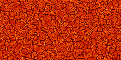
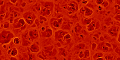
Figure 2: Vertical velocity $U_{z}$ near the surface (left panel) and near the bottom (right) of the domain from a hydrodynamical simulation. The contour levels correspond to $\pm 0.37\mbox{\rm Ma}$ (left) and $\pm 0.03\mbox{\rm Ma}$ (right).

3 Results

We first allow a hydrodynamic progenitor simulation to saturate after which we impose a uniform horizontal field $B_{0}\hat{\bm{e}}_{y}$ with $B_{0}/B_{\rm eq}\approx 0.3$. The vertical velocity $U_{z}$ near the surface ($z/d=0.98$) and near the bottom ($z/d=0.02$) of the domain in the hydrodynamic run are shown in Fig. 2. In forced turbulence simulations NEMPI appears when the scale separation between the forcing scale and the box size is of the order of 15 (Brandenburg et al., 2011). In our convection setup this is probably satisfied near the surface but not near the bottom of the domain.

We find that large-scale structures form within ten convective turnover times; see Fig. 3 where $\overline{B}_{y}\equiv\overline{B}_{y}(x,z)-\langle B_{y}\rangle_{xy}(z)$ is shown. The subscripts refer to averages over either only $y$ or over both horizontal directions, respectively. We remove the horizontal mean value (see the left panel of Fig 4) in order to make the horizontal variation of $\overline{B}_{y}(x,z)$ visible. The magnetic structures appear near the surface and sink on a timescale of a few tens of turnover times $\tau=(u_{\rm rms}k_{\rm f})^{-1}$, where we estimate $k_{\rm f}$ by $k_{\omega}=\omega_{\rm rms}/u_{\rm rms}$, and $\bm{\omega}=\bm{\nabla}\times{\bm{u}}$. Now the turbulent diffusion time $\tau_{\rm diff}=(\eta_{\rm t}k_{1}^{2})^{-1}$ is roughly 180 turnover times if we assume $\eta_{\rm t}=u_{\rm rms}/(3k_{\rm f})$ for the turbulent diffusivity. The maximum field strength in the concentrations is of the order of the imposed field. The elongated magnetic structures are also weakly discernible in the instantaneous magnetic field $B_{y}$, see the left panel of Fig. 5. In the vertical field $B_{z}$ from the same instant, however, it is not possible to distinguish the same structures, right panel of Fig. 5. This can due to the perfect conductor boundary condition which imposes $B_{z}=0$ a the boundary.

We define the effective magnetic pressure as $\overline{\mathcal{P}}_{\rm eff}={\textstyle{1\over 2}}(1-q_{p})\frac{\overline{B}^{2}}{B_{\rm eq}^{2}}$, where $q_{p}=-2\Delta\overline{\rho u_{y}^{2}}-\Delta\overline{\bm{b}^{2}}+2\Delta\overline{b_{y}^{2}}$, and where $\Delta$ refers to the difference between runs with and without an imposed field. In the present case a small-scale dynamo is absent and thus the magnetic correlations come only from the run with the imposed field. We find that the effective magnetic pressure $\overline{\mathcal{P}}_{\rm eff}$ is positive near the upper boundary and negative below $z/d<0.1$ with increasingly negative values towards the bottom, see the right panel of Fig. 4. The maxima of $\overline{\mathcal{P}}_{\rm eff}$ are associated with maxima of $\overline{B}_{y}$, whereas the minima of $\overline{\mathcal{P}}_{\rm eff}$ coincide with lower average values of $\overline{B}_{y}$, see Fig. 3.

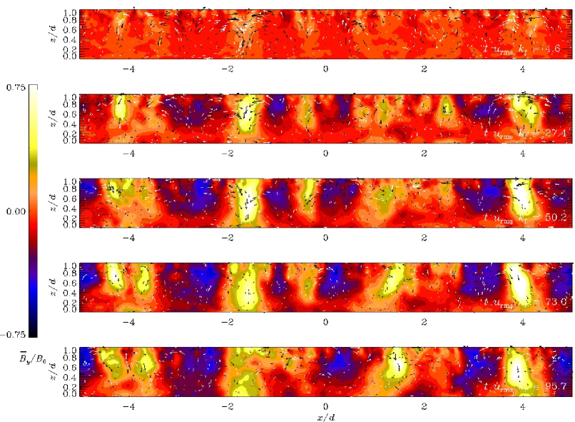
Figure 3: Mean magnetic field component $\overline{B}_{y}$ from five times separated by $23\ tu_{\rm rms}k_{\rm f}$ after initializing the magnetic field. The black and white arrows show the $y$-averaged velocity in the $(x,z)$-plane.

Figure 4: Left panel: horizontally averaged horizontal magnetic fields $\overline{B}_{x}$ and $\overline{B}_{y}$ in units of the imposed field $B_{0}$. Right panel: horizontal average of the effective magnetic pressure $\overline{\mathcal{P}}_{\rm eff}$. The average is taken over a period where the rms magnetic field is saturated.

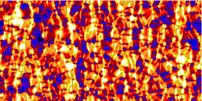
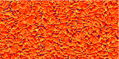
Figure 5: Magnetic field components $B_{y}$ (left panel) and $B_{z}$ (right) near the surface ($z/d=0.98$) from the same time as in the bottom panel of Fig. 3. The contour levels correspond to $-B_{0}<B_{y}-B_{0}<B_{0}$ (left) and $-B_{0}<B_{z}<B_{0}$ (right).

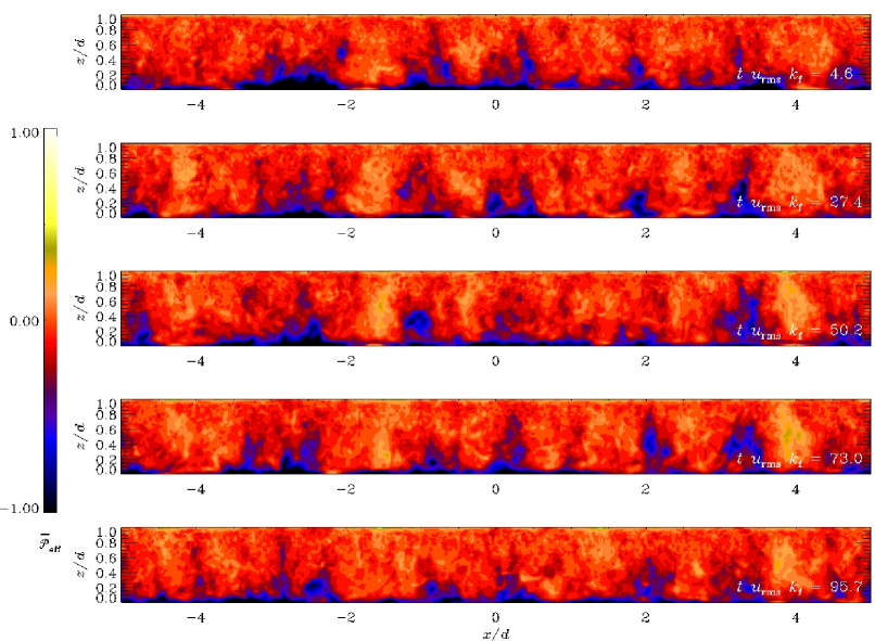
Figure 6: Effective magnetic pressure $\overline{\mathcal{P}}_{\rm eff}$ from the same times as in Fig. 3.

4 Conclusions

Our results have shown that convection can lead to magnetic flux concentrations by a mechanism that may be related to NEMPI. A possible alternative mechanism is magnetic flux expulsion that has previously been found to be responsible for a segregation of magnetised and unmagnetised regions in large aspect ratio convection simulations with an imposed vertical magnetic field (Tao et al., 1998). Our results appear to be similar, except that here we have an imposed horizontal magnetic field. In that respect, it is useful to mention recent simulations of Stein & Nordlund (2012), who inject a 1000 G horizontal magnetic field at the bottom of their simulated convection domain and find after some time the emergence of a bipolar magnetic field at the surface. In their case the reason for the formation of flux concentrations is argued to be the downdrafts of the deeper supergranulation pattern, which tend to keep the magnetic field concentrated into flux bundles at the bottom of their open domain. Our present simulations do not capture this effect, because they are probably not deep enough and our domain is impenetrative and perfectly conducting at the bottom, excluding therefore their mechanism as a possible explanation. Of course, another important difference between our simulations and those of Stein & Nordlund (2012) is the presence of a radiating surface in their case. This might enhance magnetic flux concentrations formed through local suppression of convective energy flux by magnetic fields (Kitchatinov & Mazur, 2000). This might well be an important effect that needs to be studied more thoroughly.