Bayesian modeling and forecasting of 24-hour high- frequency volatility: A case study of the financial crisis

Abstract

This paper estimates models of high frequency index futures returns using ‘around the clock’ 5-minute returns that incorporate the following key features: multiple persistent stochastic volatility factors, jumps in prices and volatilities, seasonal components capturing time of the day patterns, correlations between return and volatility shocks, and announcement effects. We develop an integrated MCMC approach to estimate interday and intraday parameters and states using high-frequency data without resorting to various aggregation measures like realized volatility. We provide a case study using financial crisis data from 2007 to 2009, and use particle filters to construct likelihood functions for model comparison and out-of-sample forecasting from 2009 to 2012. We show that our approach improves realized volatility forecasts by up to 50% over existing benchmarks.

1 Introduction

Financial crises are a rich information source to learn about asset price dynamics and models used to capture these dynamics. For example, the 1987 Crash and 1998 LTCM hedge fund crisis highlighted the importance of stochastic volatility (SV) and jumps, in both prices and volatility, for understanding index returns (see, e.g., Bates, 2000; Duffie, Pan and Singleton, 2000; Eraker, Johannes and Polson, 2003; Todorov, 2011) The recent crisis provides similar opportunities largely due to two unique features. First, unlike the 1987 or 1998 crises which were short-lived, the recent crisis began in mid 2007 and lasted well into 2009, with aftershocks into the European debt crisis and Flash-Crash in 2010. Second, structural changes in the mid 2000s led to continuous around-the-clock markets, as markets migrated from traditional floor execution during ‘regular’ market hours to fully electronic 24-hour trading. For the first time, there is ‘around the clock’ high frequency data in a long-lasting crisis.

This paper uses newly available data to study a range of important questions. What sort of models and factors are required to accurately model 24-hour high-frequency crisis returns? Do these specifications generate dynamics similar to extant ones? How useful are these models for practical applications like return distribution and volatility forecasting or trading? Answers to these questions are important for academics, policy makers, market participants and risk managers who need to understand the structure of financial market volatility and to quantify the likelihood of potential future market movements. In particular, nearly every practical finance application – including optimal investments and trading, options/derivatives pricing, market making and market microstructure, and risk management – requires volatility forecasts.

Our case study focuses on the S&P 500 index, arguably the world’s most important asset market, using S&P 500 index futures, which trade 24 hours a day from Sunday evening to Friday night. We focus on in-sample model fitting, which allows us to learn about the underlying structure of returns, and fully out-of-sample prediction, which is important for applications. We use parametric models estimated from intraday returns, something rarely attempted due to data complexities and computational burdens. Figure 1 plots intraday and interday volatility of 5-minute S&P 500 futures returns from March 2007 to March 2012. Intraday volatility has complicated, periodic patterns driven by the global migration of trading and macroeconomic announcements (see e.g. Andersen and Bollerslev, 1997, 1998). Interday volatility is persistent, stochastic, and mean-reverting. Models capturing these components require multiple volatility factors, complicated shocks, and many parameters, which, in conjunction with huge volumes of high-frequency data, make parametric estimation difficult.

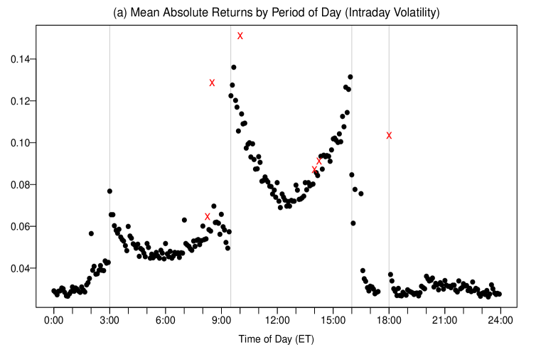
Figure 1: Summary of five-minute returns on S&P E-mini futures prices, March 2007 – March 2012. (a) Mean absolute returns for each period of the day. The trading day runs from 18:00 ET–17:30 ET, with a break in trading from 16:15–16:30. Macroeconomic announcement times are marked with an ’x’, and selected major market open and closing times are marked with vertical lines. (b) Mean absolute returns by date.

Due to these complexities, most researchers use nonparametric ‘realized volatility’ (RV) methods to avoid directly modeling intraday returns by aggregating intraday data into a daily RV measure (see Andersen and Benzoni, 2009; Barndorff-Nielsen and Shephard, 2007, for reviews). One weakness is its nonparametric nature: RV approaches generally do not specify a full model of returns, which limits practical usefulness as there is no return distribution, just volatility estimates. Despite this weakness, RV methods are extremely useful and are a popular volatility forecasting approach.

Methodologically, we build new models with the flexibility to fit the complexities of 24-hour intraday data during the financial crisis. We develop novel MCMC algorighms to fit models in-sample and use particle filters to compute predictive distributions and volatility forecasts for out-of-sample validation. Although SV models are commonly implemented with MCMC, we know of no applications using realistic SV models and intraday data for out-of-sample validation.

We find strong in and out-of-sample evidence for multiscale volatility with distinct ‘fast’ and ‘slow’ factors. The slow factor’s half-life is about 25 days, similar to extant estimates from daily data. The fast factor, however, operates intradaily, with a half-life of an hour, capturing the ‘digestion’ time of high-frequency news or liquidity events. Our models offer a significant improvement over traditional GARCH models estimated on intraday data. We find strong evidence for jumps (in prices and volatility) or fat-tails generated by t-distributed return shocks. Price jumps are rather small in comparison to estimates from earlier periods or option prices which identify jumps as large negative ‘crashes.’ This could be unique to the recent crisis or something more fundamental uncovered from newly available high frequency data. A striking and important features of our analysis is a strong and uniform ranking of models both in and out-of-sample based on predictive likelihoods.

The ultimate test of a model is usefulness, and we consider three practical applications: volatility forecasting, tail risk management, and a trading application. We compare our models’ performance to popular GARCH and RV benchmarks. In forecasting volatility, our SV models generate significantly lower forecasting errors than all competitors at all horizons. The absolute performance is striking as we generate fully out-of-sample volatility forecasts with R²’s in excess of 70%. Our SV models perform relatively and absolutely well in a quantitative risk management application–evaluating the accuracy of value-at-risk (VaR) forecasts, essentially tail forecasting–and a simple volatility trading application. Overall, we find strong evidence for the usefulness of our models and approach in all cases.

2 Data, modeling and estimation approach

2.1 Data

This paper studies S&P 500 index futures. Two contract variants exist: the traditional ‘full-size’ contract ($250 per index point) and the ‘E-mini’ contract ($50 per point). E-minis trade electronically on the Chicago Mercantile Exchange’s (CME’s) Globex platform and initially complemented the full-sized contract, which traded in a traditional ‘open outcry’ pit. E-mini trading volumes increased steadily before expanding rapidly in 2007 (see CME Group, Labuszewski, Nyhoff, Co and Petersen, 2010) with the advent of algorithmic high-frequency trading and increased global influences. S&P 500 futures are one of the most liquid contracts in the world, limiting any microstructure effects (see, e.g., Corsi, Mittnik, Pigorsch and Pigorsch, 2008).

We analyze 5-minute data from March 11, 2007 through March 9, 2012, consisting of 352,887 5-minute observations over 1293 days. The price data is for quarterly contracts, which are converted to a ‘continuous contract’ by rolling contracts two weeks before expiration. The first two years are used for parameter estimation and the remaining for forecasting. March 2007 is a natural starting date as it coincides with the dramatic trading volume increase. Trading starts on Sunday night at 18:00 and continues until 16:15 Friday (all times are Eastern). Markets close Monday-Thursday from 16:15-16:30 and from 17:30-18:00. Sunday ‘open’ returns are from Friday at 16:15 to Sunday at 18:00. There are similar ‘open’ returns from 16:15-16:30 and 17:30-18:00. Normal days have 279 return observations.

2.2 Stochastic volatility models

We model 5-minute logarithmic price returns, $y_{t}$, which evolve via

$$y_{t}=100\cdot\log\left(P_{t}/P_{t-1}\right)=\mu+v_{t}\varepsilon_{t}^{\ast}+J_{t}Z_{t}^{y}\text{,}$$

where $P_{t}$ is the futures price, $\mu$ is the mean return, $v_{t}$ is diffusive or non-jump volatility, $J_{t}$ is a jump indicator with $P\left[J_{t}=1\right]=\kappa$, $Z_{t}^{y}\overset{i.i.d.}{\sim}\mathcal{N}(\mu_{y},\sigma_{y}^{2})$ are return jumps, and $\varepsilon_{t}^{\ast}=\sqrt{\lambda_{t}}\varepsilon_{t}$ where $\varepsilon_{t}\overset{i.i.d.}{\sim}\mathcal{N}(0,1)$ and $\lambda_{t}\overset{i.i.d.}{\sim}\mathcal{IG}\left(\nu/2,\nu/2\right)$, which implies $\varepsilon_{t}^{\ast}\overset{i.i.d.}{\sim}t_{v}\left(0,1\right)$. At this level, the model resembles common jump-diffusion specifications.

There is strong evidence for stochastic volatility and jumps in S&P 500 index prices from daily data (e.g., Eraker et al., 2003), index option prices (Bakshi, Cao and Chen, 1997; Bates, 2000; Duffie, Pan and Singleton, 2000), and intraday data (Andersen and Shephard, 2009, provide a review). Estimates from options or daily returns identify large jumps or ‘crashes.’ Studies using recent high frequency data tend to find smaller jumps, though these studies typical ignore overnight periods.

We model total volatility via a multiplicative specification:

$$v_{t}=\sigma\cdot X_{t,1}\cdot X_{t,2}\cdot S_{t}\cdot A_{t}\text{,}$$ (1)

where $X_{t,1}$ and $X_{t,2}$ are SV processes, and $S_{t}$/$A_{t}$ are seasonal/announcement components. $\sigma$ is interpreted as the modal volatility (i.e. $v_{t}$ when $X_{t,1}=X_{t,2}=S_{t}=A_{t}=1$). The log of total diffusive variance is linear:

$$h_{t}=\log(v_{t}^{2})=\mu_{h}+x_{t,1}+x_{t,2}+s_{t}+a_{t},$$ (2)

where $\mu_{h}=\log(\sigma^{2})$, $x_{t,i}=\log(X_{t,i}^{2}),s_{t}=\log(S_{t}^{2})$, and $a_{t}=\log(A_{t}^{2})$.

Volatility evolves stochastically via

$$x_{t+1,1}=\phi_{1}x_{t,1}+\sigma_{1}\eta_{t,1}\text{ and }x_{t+1,2}=\phi_{2}x_{t,2}+\sigma_{2}\eta_{t,2}+J_{t}Z_{t}^{v},$$

where $\eta_{t,i}\overset{i.i.d.}{\sim}\mathcal{N}(0,1)$ and $Z_{t}^{v}\overset{i.i.d.}{\sim}\mathcal{N}(\mu_{v},\sigma_{v}^{2})$ are the jumps in log-volatility. Notice the volatility jump times are coincident with those in returns. $\rho=corr(\varepsilon_{t},\eta_{t,2})$ captures diffusive “leverage” effects via correlated shocks to returns and fast volatility. We assume a multiscale volatility specification, assuming $0<\phi_{2}<\phi_{1}<1$, with $X_{t,1}$ and $X_{t,2}$ the ‘slow’ and ‘fast’ volatility factors, respectively. Both factors are affected by intraday shocks, relaxing a common assumption that stochastic volatility is constant intraday (see, e.g., Andersen and Bollerslev, 1997, 1998).

We model the seasonal/periodic and announcement effects as deterministic volatility patterns using the spline approach in Weinberg, Brown and Stroud (2007). The seasonal component is $s_{t}=f_{t}^{\prime}\beta$, where $f_{t}=(f_{t1},...,f_{t,288})^{\prime}$ is an indicator vector where $f_{tk}=1$ if time $t$ occurs at period of the day $k$ and zero otherwise, and $\beta=(\beta_{1},...,\beta_{288})^{\prime}$ are the seasonal coefficients. We impose the constraint $\sum\nolimits_{k=1}^{288}\beta_{k}=0$ for identification. To incorporate smoothness in the seasonal coefficients we assume a cubic smoothing spline prior for $\beta$, with discontinuities at market opening/closing times. Following Wahba (1978) and Kohn and Ansley (1987), we write this as a multivariate normal prior $\beta\sim\mathcal{N}(0,\tau_{s}^{2}U_{s})$, where $\tau_{s}^{2}$ is the smoothing parameter and $U_{s}$ is a known correlation matrix (see Appendix C).

The announcement component is $a_{t}=\sum_{i=1}^{n}I_{ti}^{\prime}\alpha_{i}$, where $I_{ti}=(I_{ti1},...,I_{ti5})^{\prime}$ is an indicator vector for news type $i$ with $I_{tik}=1$ if a news release occurred at period $t-k$ and zero otherwise, and $\alpha_{i}=(\alpha_{i1},...,\alpha_{i5})^{\prime}$ are the announcement effects for news type $i$. We again assume cubic smoothing spline priors to smooth the coefficients, $\alpha_{i}\sim\mathcal{N}(0,\tau_{a}^{2}U_{a})$ (see Appendix C). We consider $n=14$ announcement types listed in Table 9 in the Appendix. We assume that announcements increase market volatility for $K=5$ periods, i.e., markets digest the news in 25 minutes. Sunday open is treated as an announcement.

Our model applies to all 5-minute intraday returns, not just those ‘traditional’ trading hours from 9:30 to 16:00. Existing papers often either ignore or simplistically correct for overnight returns. For example, Engle and Sokalska (2012), following “common practice,” delete overnight returns due either to a lack of overnight data (for individual stocks) or difficulties in modeling overnight returns, which requires both periodic and announcement components. Ignoring overnight returns is problematic for 24-hour, global markets and crisis periods. For example, on October 24, 2008, S&P 500 futures fell over 6 percent overnight, and deleting this period would remove important information.

2.3 Estimation approach

We take a Bayesian approach and use MCMC to simulate from the posterior distribution,

$$p\left(z^{T},\beta,\alpha,\theta,|y^{T}\right)\,\propto\prod_{t=1}^{T}\,p(y_{t}|z_{t},\beta,\alpha,\theta)\,p(z_{t}|z_{t-1},\theta)\,p(\beta|\theta)\,p(\alpha|\theta)\,p(\theta),$$

where $z_{t}=\left(x_{t,1},x_{t,2},\lambda_{t},J_{t},Z_{t}^{y},Z_{t}^{v}\right)$, $z^{T}=\left(z_{1},...,z_{T}\right)$, $\theta$ are parameters and $y^{T}=\left(y_{1},...,y_{T}\right)$ are returns. Appendices A and D detail the priors and algorithm, respectively. We use standard conjugate priors where possible and in all cases proper, though not strongly informative, priors. Efficiently programmed in C, the MCMC algorithm makes 12,500 draws in 12–25 minutes using a 2.8 GHz Xeon processor for each year of 5-minute returns (around 70,500 observations). Computing time is approximately linear for the sample sizes considered.

Our algorithm is highly tuned using representation and sampling ‘tricks.’ We express the model as a linear, but non-Gaussian system and use the Carter and Kohn (1994) and Frühwirth-Schnatter (1994) forward-filtering, backward sampling algorithm for block updating, an approach first used for SV models in Kim, Shephard and Chib (1998). When possible, parameters and states are drawn together. Following Ansley and Kohn (1987), we express the splines as a state space model and update in blocks. Building on the methodology of Johannes, Polson and Stroud (2009), we use auxiliary particle filters (Pitt and Shephard, 1999) to approximately sample from $p\left(z_{t}|y^{t},\widehat{\theta}\right)$, where $\widehat{\theta}$ is the posterior mean. Appendix E provides details.

It is useful to contrast our intraday parametric estimation approach to Andersen and Bollerslev (1997, 1998), the main competitor. They model 5-minute exchange rates via long-memory GARCH models with seasonal effects (see also Martens, Chang and Taylor, 2002) and use a two-step procedure to first estimate daily volatility, assumed constant intraday, and then estimate a flexible seasonal component. Engle and Sokalska (2012) estimate GARCH models on intraday returns for 2500 individual stocks with a seasonal component using third-party interday volatility estimates. By contrast, we simultaneously estimate all parameters and states, avoiding the need for potentially inefficient two-stage estimators and restrictive assumptions like normally distributed shocks and the absence of jumps.

Another approach aggregates intraday returns into daily RV statistics, which are used to estimate models at a daily frequency (see, e.g., Barndorff-Nielsen and Shephard, 2002; Todorov, 2011). We estimate the models directly on 5-minute returns, without aggregation into RV, which allows us to identify intraday components and forecast at high frequencies. Hansen et al. (2012) introduce a hybrid model, called Realized GARCH (RealGARCH), combining the tractability of daily GARCH models with the information in realized volatility. We implement these promising models and compare their performance to our SV models.

Appendix D provides algorithm details, with diagnostics in the web Appendix. The MCMC algorithms mix quite well given the large number of unknown states and parameters, although models with jumps in volatility mix more slowly than those with only diffusive volatility, and volatility of volatility parameters mix relatively slowly. Parameters deep in the state space (e.g., volatility of volatility) tend to traverse the state space more slowly, consistent with multiple layers of smoothing (see, e.g., Kim et al., 1998). This does not mean that these parameters are not accurately estimated, as simulation evidence does indicate they can be accurately estimated. The only model with any substantive concern is the SVCJ₂ model, and we thin the samples to alleviate any concerns. We have also considered significantly less informative priors and the results do not substantially change.

2.4 Decompositions and Diagnostics

To decompose variance and to quantify relative importance, we compute the posterior mean for the total log variance and for each variance component at each time period, e.g., $\overline{x}_{t,1}=E\left[x_{t,1}|y^{T}\right]$, run univariate regressions of the form $\overline{h_{t}}=\alpha+\beta\overline{x}_{t,1}+\varepsilon_{t}$, and report $R^{2}$’s for each component. We report decompositions in both log-variance and in volatility units.

To quantify model fit, we would ideally use the Bayes factor, $\mathcal{B}_{i,j}^{t}=\mathbb{P}\left[\mathcal{M}_{i}|y^{t}\right]/\mathbb{P}\left[\mathcal{M}_{j}|y^{t}\right],$ where $\left\{\mathcal{M}_{i}\right\}_{i=1}^{M}$ indicate models, $\mathbb{P}\left[\mathcal{M}_{i}|y^{t}\right]\propto p\left(y^{t}|\mathcal{M}_{i}\right)\mathbb{P}\left(\mathcal{M}_{i}\right)$, and $p\left(y^{t}|\mathcal{M}_{i}\right)$ is the marginal likelihood. Bayes factors are often called an “automated Occam’s razor,” as they penalize loosely parameterized models (Smith and Spiegelhalter, 1980). Computing marginal likelihoods requires sequential parameter estimation, which is computationally prohibitive, so we alternatively report log-likelihoods and the Bayesian Information Criterion (BIC) statistic, which approximates the Bayes factor.

The model $\mathcal{M}_{i}$ likelihood of $y^{T}$ is

$$\mathcal{L}\left(y^{T}|\theta_{\left(i\right)},\mathcal{M}_{i}\right)=\prod\nolimits_{t=0}^{T-1}p\left(y_{t+1}|\theta_{\left(i\right)},y^{t},\mathcal{M}_{i}\right),$$

where $\theta_{\left(i\right)}$ are the parameters in $\mathcal{M}_{i}$, $p\left(y_{t+1}|\theta_{\left(i\right)},y^{t},\mathcal{M}_{i}\right)$ is the predictive return distribution,

$$p\left(y_{t+1}|\theta_{\left(i\right)},y^{t},\mathcal{M}_{i}\right)=\int p\left(y_{t+1}|\theta_{\left(i\right)},z_{t+1},\mathcal{M}_{i}\right)p\left(z_{t+1}|\theta_{\left(i\right)},y^{t},\mathcal{M}_{i}\right)dz_{t+1},$$

$p\left(y_{t+1}|\theta_{\left(i\right)},z_{t+1},\mathcal{M}_{i}\right)$ is the conditional likelihood, and $p\left(z_{t+1}|\theta_{\left(i\right)},y^{t},\mathcal{M}_{i}\right)$ is the state predictive distribution. Given approximate samples from $p\left(z_{t}|y^{t},\widehat{\theta}_{\left(i\right)},\mathcal{M}_{i}\right)$, it is easy to approximately sample from the predictive distributions and likelihoods. All distributions can be computed at 5-minute and lower frequencies, such as hourly or daily, via simulation.

Defining the dimensionality of $\theta_{\left(i\right)}$ as $d_{i}$ in model $\mathcal{M}_{i}$, the BIC criterion is

$$BIC_{T}\left(\mathcal{M}_{i}\right)=-2\log\mathcal{L}\left(y^{T}|\widehat{\theta}_{\left(i\right)},\mathcal{M}_{i}\right)+d_{i}\log\left(T\right)\text{.}$$

BIC and Bayes factors are related asymptotically $BIC_{T}\left(\mathcal{M}_{i}\right)-BIC_{T}\left(\mathcal{M}_{j}\right)\approx-2\log\mathcal{B}_{i,j}^{T}$ (Kass and Raftery, 1995). BIC asymptotically (in $T$) approximates the posterior probability of a given model. The dimensionality or degrees of freedom are not preset for the splines, but are determined by the degree of fitted smoothness. We compute the degrees of freedom using the state-space approach of Ansley and Kohn (1987), evaluating the degrees of freedom at each iteration of the MCMC algorithm and using the posterior mean for model comparisons. Given our sample sizes, this approximation should perform well.

	SV	Return	Leverage	Return	Volatility	Seasonal	Announcement
Model	Factors	Errors	Effect	Jumps	Jumps	Effects	Effects
SVi	$i$	Normal				x	x
ASVi	$i$	Normal	x			x	x
SVti	$i$	Student-t	x			x	x
SVJi	$i$	Normal	x	x		x	x
SVCJi	$i$	Normal	x	x	x	x	x

Table 1: Mnemonics for the stochastic volatility models that we consider. Here, $i=$ 1 or 2.

For comparisons, we also estimated benchmark GARCH models including a GARCH(1,1) model (GARCH), and two models that incorporate asymmetry: the GJR model (Glosten, Jagannathan and Runkle, 1993), and the EGARCH model (Nelson, 1991), each with both normal and t-errors fit as in Andersen and Bollerslev (1997). Appendix G provides details.

3 Empirical results

3.1 In-sample model fits

Table 1 describes the models considered. We estimated single-factor models, but do not report estimates as the 2-factor models always performed better in and out-of-sample. Table 2 reports in-sample fit statistics including the degrees of freedom, log-likelihoods, and BIC statistics. To ease comparisons, Table 2 reports Bayes factors based on the difference of BIC statistics relative to the $SV_{1}$ model, $-2\log\mathcal{B}_{i,SV_{1}}=BIC_{T}\left(\mathcal{M}_{i}\right)-BIC_{T}\left(\mathcal{M}_{SV_{1}}\right)$. Better fitting models have higher likelihoods and lower BIC statistics, quantifying the improvement over a single-factor SV model.

Degrees of freedom range from 253 to 284. This consists of ‘static’ parameters $d^{\ast}$ (from 4 to 12) and the spline ‘parameters,’ $d_{s}$ and $d_{a},$ which are less than the number of knot points (279 and 70, respectively) and determined by the spline’s smoothness. More complicated models sometimes have fewer degrees of freedom than their simpler counterparts, even though they have more static parameters. The multiscale, two-factor SV models provide the best in-sample fits and, in all cases, the BIC and log-likelihood statistics provide the same conclusion, which is not surprising given the large samples. The best performing models, the SVt₂ and SVCJ₂ models, have leverage effects and allow for outliers, via either jumps or $t-$distributed shocks, which are needed to fit the fat-tails of intraday returns.

	$d^{*}$	$d_{s}$	$d_{a}$	$d$	$\log\mathcal{L}$	BIC	$-2\log\mathcal{B}_{ij}$
GARCH	3	279	0	282	192558	-381775	10584
GARCH-t	4	279	0	283	197725	-392097	262
GJR	4	279	0	283	192662	-381969	10390
GJR-t	5	279	0	284	197795	-392224	135
EGARCH	4	279	0	283	192459	-381564	10795
EGARCH-t	5	279	0	284	197759	-392153	206
SV2	6	210	51	267	198788	-394424	-2065
ASV2	7	210	51	268	198865	-394566	-2207
SVt2	8	196	51	255	199235	-395461	-3102
SVJ2	10	191	52	253	198958	-394929	-2570
SVCJ2	12	189	52	254	199214	-395429	-3070

Table 2: Degrees of freedom, log-likelihoods, BIC statistics and approximate log Bayes Factors for each model (relative to the SV₁ model) for the estimation period, March 2007–March 2009.

The multiscale SV models provide significant improvements in fits compared to the GARCH models. In fact, the Bayes factors indicate that a simple 1-factor SV model actually outperforms all of the GARCH models, strong evidence supporting SV. This indicates there is something fundamental about the random nature of volatility in the SV–the extra shock in the volatility evolution–that improves the fit, which can be compared to the GARCH models in which the shocks to volatility are completely driven by return shocks.

We can not compare likelihood-based fits to RV based models which typically do not specify an intraday return distribution. We also fit variants omitting seasonalities and/or announcements, which are not reported to save space. Both components are significant, though the announcement components are less important given the relatively small number of announcements per week.

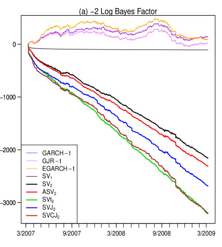
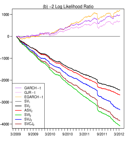
Figure 2: (a) Cumulative log Bayes factors during the in-sample period, March 2007–March 2009. (b) Cumulative log-likelihood ratios during the out-of-sample period, March 2009–March 2012. Values are relative to the SV₁ model, and are multiplied by -2, so lower values indicate better fit.

West (1986) suggests monitoring model fits sequentially through time to provide an assessment of model failure, either abruptly or slowly over time. Figure 2a reports in-sample sequential Bayes factors for each model relative to the SV₁ model, $BIC_{T}\left(\mathcal{M}_{i}\right)-BIC_{T}\left(\mathcal{M}_{SV_{1}}\right)$. Note the gradual outperformance generated by the SVCJ₂ and SVt₂ models, indicating general fit improvement and not one generated by a very small number of observations. The relative ranking of the SV models is identical out-of-sample, confirming the in-sample results.

There is one noticeable spike on October 24, 2008 in the log Bayes factors. This was caused by a circuit breaker locking S&P 500 futures limit down from 4:55 am to 9:30 a.m., which generated a number of zero returns. Exchange rules mandate that S&P futures can not fall by more than 60 points overnight and trading can occur at prices above, but not below, this level until 9:30. Models with fast-moving volatility were able to reduce their predictive volatility quickly, thus the relatively good fit during this event. A more complete specification would incorporate a mechanism for limit down markets.

3.2 Parameter estimates, variance decompositions and sample paths

Table 3 summarizes the posteriors and reports inefficiency factors and acceptance probabilities (for the slowest mixing component, $\sigma_{1}$) for the multiscale models. There are a number of interesting results. The SV factors correspond to a slow-moving interday factor and rapidly moving intraday factor. Estimates of $\phi_{1}$ in the best fit models are 0.9999, corresponding to a daily AR(1) coefficient of 0.9725 and a half-life ($\log 0.5/\log\phi_{1})$ of almost 25 days. This is consistent with studies using daily data and time-aggregation, that is, that the data provides similar inference whether sampled at intraday or daily frequencies. $x_{t,2}$ operates at high frequencies with a 5-minute AR(1) coefficient $\phi_{2}$ of 0.926 to 0.958, generating a half-life of around an hour, and high volatility ($\sigma_{2}\gg\sigma_{1}$). Intuitively, there is strong evidence for rapidly dissipating high-frequency volatility shocks to volatility. All 2-factor models support an extreme form of multiscale SV that would be difficult to detect using daily data.

	SV2	ASV2	SVt2	SVJ2	SVCJ2
$\mu$	0.0001	0.0000	0.0000	0.0000	0.0000
	(0.0001)	(0.0001)	(0.0001)	(0.0001)	(0.0001)
$\sigma$	0.060	0.060	0.059	0.060	0.059
	(0.011)	(0.012)	(0.014)	(0.012)	(0.013)
$\phi_{1}$	0.9998	0.9998	0.9999	0.9999	0.9999
	(0.0001)	(0.0001)	(0.0000)	(0.0001)	(0.0001)
$\sigma_{1}$	0.022	0.021	0.019	0.020	0.020
	(0.001)	(0.002)	(0.002)	(0.001)	(0.001)
$\tau_{1}$	1.257	1.300	1.339	1.291	1.277
	(0.246)	(0.411)	(0.452)	(0.606)	(0.373)
$\phi_{2}$	0.927	0.929	0.957	0.946	0.945
	(0.004)	(0.004)	(0.003)	(0.003)	(0.004)
$\sigma_{2}$	0.191	0.189	0.138	0.158	0.127
	(0.005)	(0.005)	(0.005)	(0.004)	(0.005)
$\tau_{2}$	0.509	0.512	0.476	0.488	0.486
	(0.007)	(0.009)	(0.010)	(0.009)	(0.011)
$\rho$		-0.095	-0.126	-0.106	-0.136
		(0.014)	(0.017)	(0.015)	(0.019)
$\nu$			20.58
			(1.12)
$\kappa$				0.0018	0.0042
				(0.0003)	(0.0004)
$\mu_{y}$				0.060	-0.007
				(0.036)	(0.013)
$\sigma_{y}$				0.437	0.202
				(0.046)	(0.015)
$\mu_{v}$					0.816
					(0.086)
$\sigma_{v}$					1.220
					(0.069)
aprob	0.308	0.312	0.328	0.289	0.292
ineff	51.5	41.0	90.8	29.0	97.9

Table 3: Posterior means and standard deviations (in parentheses) for the two-factor models. The bottom two rows are the Metropolis-Hastings acceptance probabilities and inefficiency factors for the slowest mixing parameter, $\sigma_{1}$.

Decompositions in Table 4 show the interday factor explains a majority of total variance, thus the slow-moving factor is relatively more important than the fast-moving factor. The second factor explains about 7%-10% of the total variance. Table 3 reports each volatility factor’s unconditional variance, defined as $\tau_{i}^{2}$. $\tau_{1}$ is more than twice as large as $\tau_{2}$, driven by the near unit root behavior of $x_{t,1}\$and despite $x_{t,1}$’s low conditional volatility.

The second volatility factor plays a crucial role as it relieves a tension present in one-factor models. The SV factor in one-factor models tries to fit both low and high-frequency movements, ending up somewhere in between and fitting both poorly. For example, in the SVt₁ model, estimates of $\phi_{1}$ are roughly 0.997, corresponding to a daily AR(1) coefficient of 0.4325 and a half-life of about $0.80$ days, which is much slower than the fast factor and much faster than the slow factor in two-factor models. The two-factor specifications provide flexibility allowing the factors to fit higher and lower frequency volatility fluctuations.

		Log Variance					Volatility
		$x_{1}$	$x_{2}$	$s$	$a$		$X_{1}$	$X_{2}$	$S$	$A$
SV2		53.4	7.0	38.3	1.3		59.1	7.2	30.4	3.3
ASV2		53.5	6.8	38.4	1.3		59.1	7.1	30.5	3.3
SVt2		53.5	6.4	38.8	1.3		58.9	7.1	30.8	3.3
SVJ2		53.3	6.9	38.6	1.3		58.9	7.4	30.6	3.1
SVCJ2		52.1	8.6	38.0	1.2		57.0	10.2	29.7	3.2

Table 4: Volatility decomposition (percentage of total), March 2007–March 2009

Estimates of $\nu$ are about 20, consistent with mild non-normality and previous daily estimates (e.g., Chib, Nardari and Shephard, 2002; Jacquier, Polson and Rossi, 2004). Though modest, $\nu$ implies vastly higher probabilities of large shocks, some of which will occur in our massive sample. Estimates of $\rho$ are modest and around -.10. Identifying this parameter using RV is difficult due to various biases (see, e.g., Aït-Sahalia et al., 2013). Time-variation in the variance components accounts for most of the non-normality in models without jumps. Mean jump sizes, $\mu_{y},$ are close to zero in the SVCJ₂ specification, and arrivals are frequent with $\kappa=.004$ corresponding to at a rate of 1.17 per day. Return jumps are relatively large as $\sigma_{y}$ is much larger than the modal (non-jump) volatility, e.g., $\sigma_{y}=0.202$ vs. $\sigma=0.059$ in the SVCJ₂ model. Volatility jumps are quite large, with $\mu_{v}=0.816$ implying that jumps more than double 5-minute volatility.

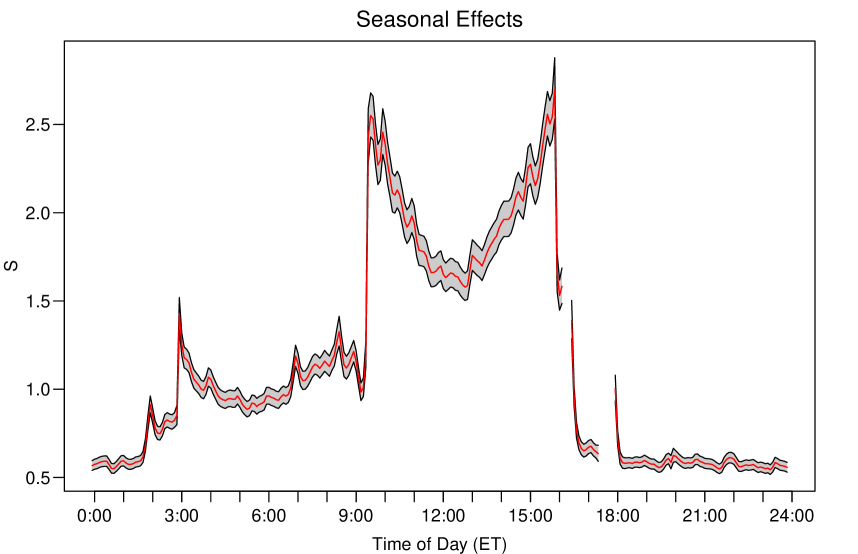
Figure 3: Posterior means and 95% intervals for the seasonal effects, $\beta=(\beta_{1},\ldots,\beta_{288})$. Results are shown on the standard deviation scale, $S=\exp(\beta/2)$. For example, a value of $S=2$ means that volatility is twice its baseline level.

Our jump estimates are ‘big,’ as price jump volatility is about 4-8 times unconditional 5-minute return volatilities. However, the sizes are relatively small when compared to estimates from older daily price data or option prices, which find rare jumps that are large and negative. Although our sample contains some of the largest index moves ever observed in the U.S. history, these were not large discontinuous moves, but rather a large number of modest moves in the same direction. Thus, high-frequency data in the most recent crisis provides a different view of jumps.

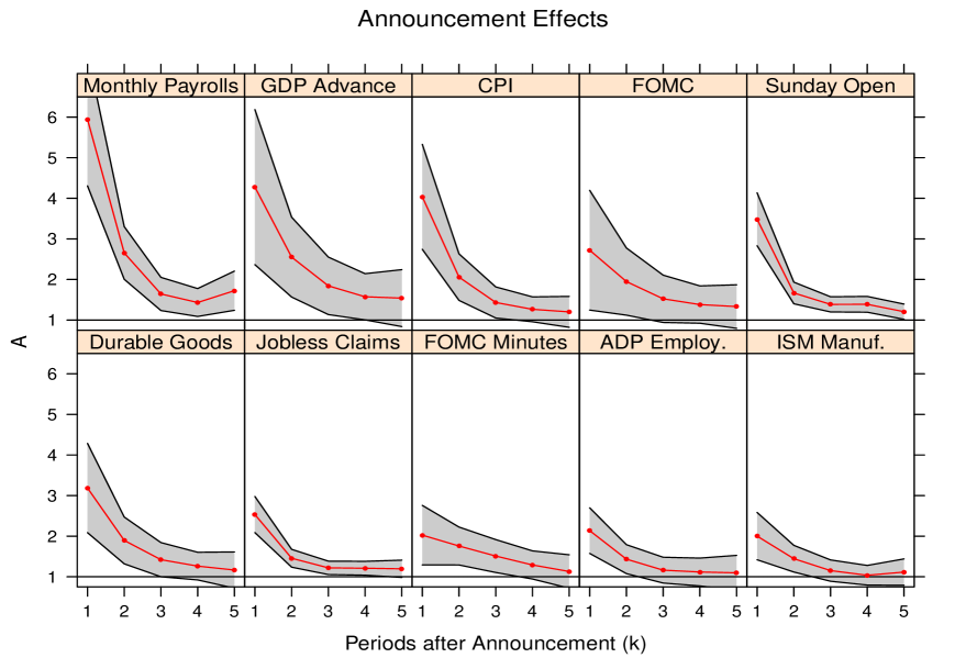
Figure 4: Posterior means and 95% intervals for the announcement effects, $\alpha_{i}=(\alpha_{i1},\ldots,\alpha_{i5})$. Results are shown on the standard deviation scale, $A=\exp(\alpha/2)$. For example, a value of $A=2$ means that volatility is twice its baseline level.

Figure 3 summarizes the posterior distribution of $S_{t}$. $S_{t}=1$ corresponds to average 5-minute volatility, so $S_{t}=0.5$ would imply that volatility is roughly half average volatility. $S_{t}$ spikes to more than 2.5 at the open and close of U.S. trading, and there is a clear ‘U’ shaped pattern during U.S. trading hours. $S_{t}$ fluctuates by a factor of more than 5, highlighting the importance of predictable intraday volatility. Figure 4 summarizes the most important announcements for the SVCJ₂ model (the other models are similar). Volatility after Payrolls increases by 6 times, with the GDP, CPI and FOMC announcements the next most important, with volatility increases of 3-4 times. The rate of decrease for the FOMC announcements are slower than for Payrolls, consistent with a greater digestion time.

To understand interday volatility, Figure 5 plots daily returns, daily RV, and the slow volatility $\sigma X_{t,1}$. Volatility spiked first in August 2007, with the panic in short-term lending markets. Additional spikes occurred after the FOMC announcement in January 2008 and the Bear Stearns takeover by J.P. Morgan in March 2008. Markets calmed down until Fall 2008, when the crisis elevated volatility to its highest levels: on an annualized scale, $\sigma X_{t,1}$ was about 60%. The slow factor closely mirrors daily realized volatility.

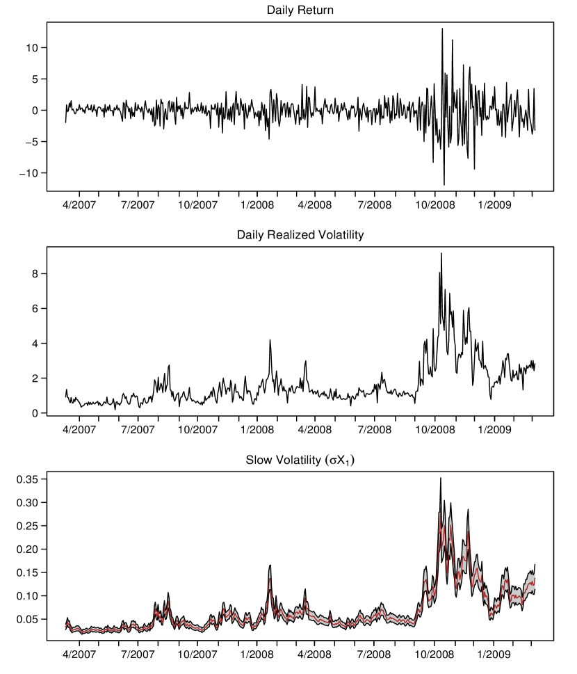
Figure 5: Daily returns, realized volatility, and smoothed means and 95% intervals for the slow volatility component, $\sigma X_{1}$, for the SVCJ₂ model, March 2007–March 2009.

To understand higher-frequency movements, Figure 6 plots the smoothed state variables during the week of September 14, 2008 for the SVCJ₂ model, when the following happened: on September 14, Lehman Brothers filed for bankruptcy; on September 15, a large money market fund ‘broke the buck’; on September 16, AIG was bailed out, there was an FOMC meeting, and Bank of America announced their purchase of Merrill Lynch; and on September 18, the SEC banned short-selling of financial stocks. The Sunday night overnight return was -2.75%, as markets digested the Lehman news. The model captures this move via a jump and elevated intraday and interday volatility–interday volatility was more than twice its long run average. On September 16, an FOMC announcement generated huge volatility with three 5-minute returns greater than 1%. Despite the elevated announcement volatility, the model still needed a large jump in volatility. After the close of normal trading, there were additional volatility jumps corresponding to the Merrill Lynch merger. The large moves on September 18 were associated with rumors and the subsequent announcement of the short-selling ban on financial stocks, drove futures roughly 100 points higher overnight.

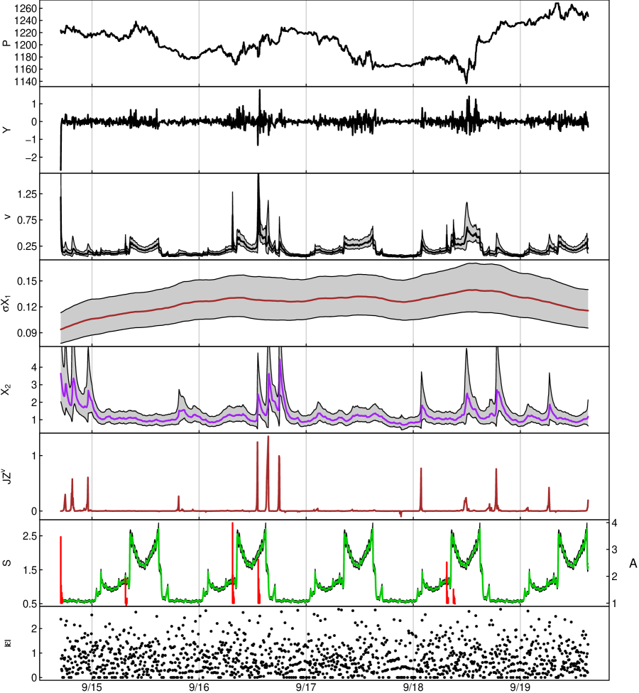
Figure 6: Prices, returns, smoothed volatility components (total volatility, slow volatility, fast volatility, volatility jumps, seasonal and announcement components) and absolute value of the residuals during the week of September 14–19, 2008 for the SVCJ₂ model. Each panel contains posterior means, and the bands represent 95% posterior intervals. The second panel from the bottom summarizes the seasonal fits on the left-hand axis and announcements on the right.

These results show the key role played by jumps in volatility and the fast volatility factor, capturing the impact of unexpected news arrivals by temporarily increasing volatility. In the SVt₂ model, large outlier shocks generated by the t-distributed errors play a similar role in explaining these large moves. Diffusive volatility is not able to increase rapidly enough to capture extremely large movements.

4 Out-of-sample results and applications

Although in-sample fits are important, the ultimate test is predictive and practical: how well does the model fit future data and can the model be used for practical applications? In terms of overall predictive ability, Figure 2b reports out-of-sample likelihood ratios relative to the SV₁ model, which are based on the entire predictive distribution and provide an overall measure of model fit. The ranking is nearly identical to the in-sample results, and the GARCH models perform very poorly out-of-sample in fitting the entire return distribution. This is strong confirmation of model performance. In terms of applications, we consider three (volatility forecasting, quantitative risk management, and a simple volatility trading example) that are described below.

4.1 Volatility forecasts

Volatility forecasting is required for nearly every financial application, as mentioned earlier, and is the gold-standard for evaluating estimators and models when using intraday data (see Andersen and Benzoni, 2009). We compare volatility forecasts from our SV models to a range of GARCH and nonparametric RV based estimators. We estimate parameters as of March 2009 and forecast volatility from March 2009 to March 2012, a challenging period for three reasons: the in-sample period is shorter than the out-of-sample period; the out-of-sample period had lower volatility; and we do not update parameters estimates.

We compute model based estimates, $\widehat{RV}_{s,\tau}^{2},$ of realized variance, $RV_{s,\tau}^{2}=\sum\nolimits_{t=1}^{\tau}y_{s+t}^{2},$ at hourly ($\tau=12$) and daily ($\tau=279)$ horizons. The 5-minute forecasts are similar to the hourly ones and are not reported. Table 5 reports forecast bias, mean-absolute forecasting errors (MAE), and forecasting regression $R^{2}$’s from Mincer-Zarnowitz regressions,

$$RV_{s,\tau}=b_{0}+b_{1}\,\widehat{RV}_{s,\tau}+\varepsilon_{s,\tau}.$$

		1 Hour				Daily
		Bias	MAE	$R^{2}$		Bias	MAE	$R^{2}$
EWMA		-0.012	0.068	59.0		0.129	0.314	49.7
GARCH		-0.024	0.073	56.8		-0.177	0.321	49.2
GARCH-t		-0.016	0.071	56.4		-0.169	0.320	47.2
GJR		-0.023	0.072	57.4		-0.166	0.316	48.8
GJR-t		-0.016	0.070	56.9		-0.156	0.316	46.8
EGARCH		-0.028	0.072	61.3		-1.132	1.146	57.5
EGARCH-t		-0.018	0.068	60.6		-0.491	0.543	57.4
SV2		-0.006	0.061	66.2		-0.048	0.201	73.5
ASV2		-0.005	0.060	66.4		-0.050	0.205	72.4
SVt2		-0.004	0.060	66.5		-0.053	0.204	72.1
SVJ2		-0.007	0.060	66.4		-0.077	0.212	72.7
SVCJ2		-0.007	0.060	66.1		-0.090	0.216	73.5
AR-RV∗						-0.090	0.229	69.0
AR-RV†						0.013	0.208	67.5
RealGARCH∗						-0.571	0.616	61.6
RealGARCH†						-0.082	0.226	68.7

Table 5: Out-of-sample predictions for hourly and daily realized volatility. The AR-RV and RealGARCH models are estimated using daily data. $*$ and $\dagger$ indicate models fit on the linear and log-linear scale, respectively. All other models are estimated using 5-minute data.

The SV models outperform all competitors. Compared to intraday GARCH, the SV models provide a lower bias, lower MAE, and higher R²’s. The SV models generate daily R²’s of 73%, an almost 50% improvement compared to R²’s of 47% to 57% for the GARCH specifications. This is a remarkably high level of predictability. At hourly horizons, R², are more than 10% higher (e.g., R²’s from 56%-60% to 66%). All of the SV models provide broadly similar fits, indicating that differences in log-likelihoods are largely due to tail fits. We also benchmark to the RV-based long-memory autoregressive (AR-RV) model of Andersen et al. (2003), and the Realized GARCH model of Hansen et al. (2012). These competitors are computed only at the daily horizon, following the literature. Our SV models generate higher R²’s in every case, and the SV models’ MAE and bias are generally similar or lower. The RV based models clearly outperform the basic GARCH models.

		1 Hour			Daily
		$b_{1}$ ($t$)	$b_{2}$ ($t$)		$b_{1}$ ($t$)	$b_{2}$ ($t$)
EWMA		0.00 ( 0.09)	0.91 (61.84)		0.06 ( 2.12)	0.90 (26.55)
GARCH		-0.02 (-1.74)	0.93 (70.85)		0.08 ( 2.35)	0.90 (26.91)
GARCH-t		-0.02 (-1.69)	0.93 (72.58)		0.07 ( 2.06)	0.91 (27.90)
GJR		-0.00 (-0.34)	0.91 (68.56)		0.10 ( 3.08)	0.88 (27.27)
GJR-t		-0.00 (-0.28)	0.91 (70.31)		0.09 ( 2.73)	0.89 (28.23)
EGARCH		-0.01 (-0.83)	0.92 (51.04)		0.11 ( 2.88)	0.86 (21.94)
EGARCH-t		-0.00 (-0.30)	0.92 (54.43)		0.15 ( 3.08)	0.86 (22.06)
AR-RV∗					0.19 ( 2.75)	0.79 (11.91)
AR-RV†					0.08 ( 1.09)	0.89 (13.39)
RealGARCH∗					-0.03 (-0.36)	0.98 (18.68)
RealGARCH†					0.04 ( 0.60)	0.91 (11.88)

Table 6: Bivariate ’horse-race’ regressions for realized volatility using the model in Equation (3). $b$ and $t$ represent the estimated regression coefficients and corresponding $t$ statistics. AR-RV and RealGARCH models are estimated using daily data. $*$ and $\dagger$ indicate models fit on the linear and log-linear scale, respectively. All other models are estimated using 5-minute data.

To attach statistical significance, we run bivariate ‘horse-race’ regressions,

$$RV_{s,\tau}=b_{0}+b_{1}\,\widehat{RV}_{s,\tau}+b_{2}\,\widehat{RV}_{s,\tau}^{SVCJ}+\varepsilon_{s,\tau},$$ (3)

where $\widehat{RV}_{s,\tau}$ is from a competitor model and $\widehat{RV}_{s,\tau}^{SVCJ}$ is from the SVCJ₂ model. Table 6 summarizes the results. Hourly, SVCJ₂ forecasts are highly significant (t-statistics greater than 50) in every case, and the competitors are insignificant in every case. The SVCJ₂ coefficients are close to but slightly less than one, and GARCH coefficients are near zero. Daily SVCJ₂ forecasts are also highly significant in every case, with t-statistics ranging from 12 to almost 30. Interestingly, competitor forecasts are significant in many cases, though less so than the SVCJ₂ forecasts. Economically, $b_{2}$ estimates are close to one and those for the competitor models are close to zero. There is some incremental information in some of the other models, as they are significant in a number of cases, which suggests there is additional predictability to be harvested. It would be interesting to consider an SV model that treats lagged RV as a ‘regressor’ variable, in a manner similar to the Realized GARCH model.

Overall, the results provide additional confirmation to Hansen and Lunde (2005)’s important paper, which finds that it is possible to outperform simple GARCH(1,1) models. Parametric SV models provide strong improvements in forecasting ability, even in challenging periods of time.

		5-Minute					1 Hour					Daily
		1	5	10	$D$		1	5	10	$D$		1	5	10	$D$
GARCH		1.6	4.6	8.3	25		1.3	4.0	7.4	30		0.8	5.9	9.9	36
GARCH-t		1.6	4.7	8.5	24		1.2	4.2	8.0	24		0.6	6.7	11.1	36
GJR		1.6	4.7	8.4	25		1.2	4.0	7.5	30		0.6	5.8	10.0	28
GJR-t		1.6	4.7	8.5	24		1.2	4.2	8.1	23		0.8	6.4	11.1	28
EGARCH		1.5	4.4	8.0	29		1.1	3.5	6.9	33		0.0	0.5	2.1	96
EGARCH-t		1.0	4.9	9.8	13		1.0	3.8	7.5	26		0.0	2.4	6.6	47
SV2		1.3	5.0	9.4	14		1.3	4.4	8.7	17		2.1	6.4	9.8	28
ASV2		1.3	5.0	9.4	15		1.2	4.3	8.6	17		1.7	6.0	9.5	34
SVt2		1.3	5.0	9.6	14		1.3	4.3	8.6	17		1.8	6.4	9.6	31
SVJ2		1.4	5.1	9.5	14		1.1	4.2	8.5	18		1.7	5.9	9.5	31
SVCJ2		1.4	5.1	9.5	14		1.1	4.2	8.6	17		1.2	5.7	9.5	32
RealGARCH∗												1.4	4.9	8.2	41
RealGARCH†												1.7	5.0	8.1	43

Table 7: Out-of-sample lower-tail coverage probabilities (1%, 5% and 10%) and distance metrics ($D$) for 5-minute, hourly and daily returns. All values are multiplied by 100. RealGARCH models are estimated using daily data. $*$ and $\dagger$ indicate models fit on the linear and log-linear scale, respectively. All other models are estimated using 5-minute returns.

4.2 Risk management

Quantitative risk management requires models to accurately fit distributional tails in order to assess the risks of extreme losses. Regulators often mandate VaR-based risk management procedures, which are essentially real-time tail forecasts (see, e.g., Duffie and Pan, 1997). VaR is the loss in value that is exceeded with probability $p$, essentially the ‘$100-p^{th}$%’ critical value of the predictive distribution of returns. Financial institutions compute VaR at daily or lower frequencies, but intraday measures are useful for market makers, high frequency trading, and options traders. To gain intuition, Figure 7 plots realized daily returns and the 1% and 5% daily VaR for the SVCJ₂ model. VaR ranges from a low of well less than 1% to a high of almost 20% during the crisis, with few noticeable or dramatic violations.

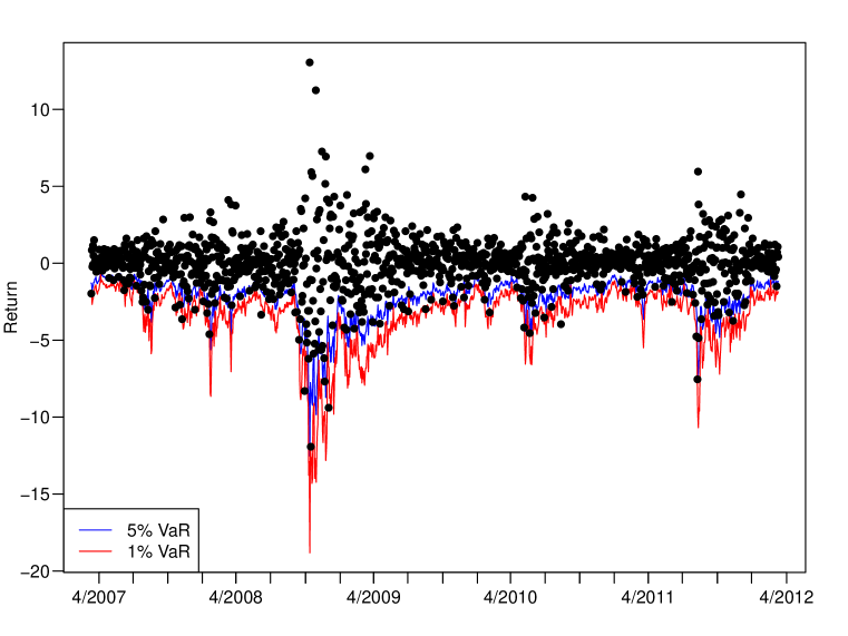
Figure 7: Daily returns and out-of-sample 1% and 5% Value-at-Risk (VaR) for daily returns for the SVCJ₂ model.

To evaluate the VaR performance out-of-sample, Table 7 reports 5-minute, 1-hour, and daily tail coverage probabilities at the 1%, 5%, and 10% levels, as well as a measure of total fit, $D$, which compares the ordered predictive quantiles of the model with observed data. The SV models generate more stable (across critical values and time horizons) and generally more accurate VaR forecasts and distributional fits, with the SVCJ₂ model performing marginally the best. Occasionally, a competitor model may perform better at one frequency and for some quantiles, but no model uniformly dominates the SV models. For example, the EGARCH-t model has the best 5-minute VaR performance, but it provides the worst at the daily frequency and performs poorly in volatility forecasting. In terms of non-GARCH competitors, the AR-RV models, due to a lack of return distribution, cannot be used for VaR calculations. The RealGARCH models do not provide intraday forecasts and, overall, the daily RealGARCH VaR statistics are generally on par or slightly worse than the best performing SV models–slightly worse at 1% level, better at the 5% level, worse at the 10% level, and worse in terms of overall fit.

Overall, the multiscale SV models provide a robust and stable fit to the tails of the return distribution over all horizons, which indicates their potential usefulness for VaR based risk management.

4.3 Volatility trading

Volatility forecasts are useful for a range of practical applications, as mentioned earlier. Documenting the economic benefits of a forecasting method is, however, quite difficult, as most applications require additional assumptions. For example, portfolio applications typically require expected return estimates and a model of investor preferences, both of which are arguably more difficult than volatility forecasting. This generates a difficult joint specification problem: if, e.g., a trading strategy does not work well, is it due to the volatility forecasts or the other components of the problem? The same holds for derivatives pricing, as one must specify risk premia and figure out how investors jointly learn about volatility from derivatives pricing and historical returns. Because of this, few papers analyze truly out-of-sample portfolio problems (see Johannes, Korteweg and Polson, 2014, for a review).

To highlight the economic value of our models while avoiding these complexities, we implement a mean-reverting trading rule. Volatility is not directly tradeable, and neither is the VIX index, but we base our trading strategy on an ETF, the VXX, which is linked to futures on the VIX index. Our trading strategy is based on volatility extremes and compares volatility forecasts from various models with the VIX index, a common measure of option implied volatility. For each model, we compute 5% and 95% predictive bands for RV, either analytically (AR-RV and RealGARCH) or via simulation (for the intraday models). If the VIX index is higher or lower than the 95% or 5% bands, respectively, we enter into mean-reversion trades in the VXX, an ETF inversely linked to the VIX index. If VIX crosses the median forecast (which changes dramatically over time), we close the position. It is important to note that the procedure is fully out-of-sample and applied symmetrically to all models.

		Single Model						Long Minus Short
		$+$	$-$	Mean	SD	SR		$+$	$-$	Mean	SD	SR
GARCH		3	129	25.4	26.6	0.95		62	325	67.8	40.3	1.68
GARCH-t		1	62	16.0	15.1	1.06		7	335	77.2	37.4	2.06
GJR		4	154	29.6	28.8	1.03		61	300	63.6	38.8	1.64
GJR-t		1	62	16.0	15.1	1.06		7	335	77.2	37.4	2.06
EGARCH		450	2	-40.0	44.0	-0.91		0	405	133.2	70.6	1.89
EGARCH-t		2	14	4.8	5.9	0.81		7	384	88.4	39.9	2.22
SV2		7	551	105.1	48.0	2.19		189	34	-11.9	29.4	-0.41
ASV2		7	532	94.5	47.0	2.01		159	23	-1.3	25.8	-0.05
SVt2		5	521	82.6	46.5	1.78		140	13	10.6	24.9	0.43
SVJ2		7	431	90.4	44.5	2.03		52	17	2.8	20.7	0.14
SVCJ2		7	396	93.2	40.2	2.32
AR-RV∗		8	0	3.2	10.2	0.32		0	397	90.0	39.5	2.28
AR-RV†		9	395	53.2	42.9	1.24		123	124	40.0	36.9	1.08
RealGARCH∗		6	0	4.7	11.8	0.40		3	398	88.5	41.5	2.13
RealGARCH†		3	461	73.9	44.4	1.66		128	59	19.3	30.2	0.64

Table 8: Out-of-sample VXX trading results, March 2009–March 2012. Trading rules are based on a single model (left panel), and a long-minus-short portfolio (right panel). $+$ and $-$ are the number of days each portfolio is long or short the index. Mean, SD and SR are the mean, standard deviation and Sharpe ratio (Mean/SD) for the portfolio returns.

The financial crisis provides an interesting laboratory since it is likely that any market inefficiencies or predictability might be magnified and thus mean-reversion trades are a natural strategy to consider. This approach has a number of other advantages: (1) it is a simple trading rule, (2) it depends crucially on volatility forecasts, and (3) it allows for a direct relative comparison of different forecasting models. Other research, e.g., Nagel (2012) has documented the value of simple mean-reversion trades during the crisis, suggestive of strong liquidity premia or over-reaction.

Table 8 reports trade summaries for each model and a long/short portfolio that goes long the trades from the SVCJ₂ model and short those from other models. Given the asymmetries in volatility–volatility tends to spike higher and mean-revert rapidly–there are many more long VXX trades (i.e., short the VIX index). The only exception is the EGARCH model, which at the daily level is strongly biased (see Table 5) and generates poor results. The other models generate positive annualized Sharpe ratios, indicative of predictive ability, but the multiscale SV models have higher Sharpe ratios than all of the competitor models. We also compute returns that are long the trading returns from the SVCJ₂ model and short another model. These Sharpe Ratios are always positive, and often on par with the Sharpe ratio for the SVCJ₂ model. This essentially removes coincident trades and focuses on trades where the models disagree. This provides additional evidence for the practical utility of our approach.

5 Conclusions

This paper develops multifactor SV models of 24-hour intraday equity index returns during and after the recent financial crisis. We estimate the models directly using MCMC methods and use particle filtering methods for forecasting and model evaluation. These models, more general than any in the literature, provide a significant improvement in-sample and out-of-sample fits, using both statistical metrics and applications.

In terms of model properties, we find strong evidence for multiscale volatility, outliers (jumps or t-errors), periodic components capturing intraday predictability, and announcements. Importantly, based on predictive likelihoods, we find the exact same ordering of models in- and out-of-sample, which indicates the results are robust and stable, even during the extreme volatility realized in the crisis. Out-of-sample, we find additional support for our approach based on superior volatility forecasts, VaR risk management, which captures tail prediction, and a volatility trading strategy.

These results are important as they document the practical usefulness of sophisticated SV models for modeling intraday returns. Our results quantify the improvements from carefully building models of intraday volatility that account for jumps, multiple volatility factors, periodic components, and announcements. SV models are not only competitive with RV or GARCH models, but actually provide significant improvements in terms of in and out-of-sample likelihood fits and applications like volatility forecasting, risk management, and volatility trading.

Appendix A: Model and Priors

The general two-factor stochastic volatility model can be written as

Log Returns: $$y_{t}=\mu+\exp(h_{t}/2)\sqrt{\lambda_{t}}\;\varepsilon_{t}+J_{t}Z_{t}^{y}$$

Total Volatility: $$h_{t}=\mu_{h}+x_{t,1}+x_{t,2}+f_{t}^{\prime}\beta+I_{t}^{\prime}\alpha$$

Slow Volatility: $$x_{t,1}=\phi_{1}x_{t-1,1}+\sigma_{1}u_{t-1,1}$$

Fast Volatility: $$x_{t,2}=\phi_{2}x_{t-1,2}+\sigma_{2}\left(\rho\varepsilon_{t-1}+\sqrt{1-\rho^{2}}u_{t-1,2}\right)+J_{t-1}Z_{t-1}^{v}$$

Periodic/Seasonal: $$\beta_{i}\sim\mathcal{N}(0,\tau_{s}^{2}U_{s})\cdot\mathbbm{1}(1^{\prime}\beta=0)$$

Announcements: $$\alpha_{i}\sim\mathcal{N}(0,\tau_{a}^{2}U_{a})$$

Scale Factors: $$\lambda_{t}\sim\mathcal{IG}(\nu/2,\nu/2)$$

Jump Times: $$J_{t}\sim\mathcal{B}ern(\kappa)$$

Return Jumps: $$Z_{t}^{y}\sim\mathcal{N}(\mu_{y},\sigma_{y}^{2})$$

Volatility Jumps: $$Z_{t}^{v}\sim\mathcal{N}(\mu_{v},\sigma_{v}^{2})$$

$U_{s}$ and $U_{a}$ are correlation matrices corresponding to the cubic smoothing spline priors, as defined in Appendix B. We assume the following prior distributions for the parameters: $\mu\sim\mathcal{N}(0,1)$, $\mu_{h}\sim\mathcal{N}(-6.2,1)$, $(\phi_{i}+1)/2\sim\mathcal{B}(20,1.5)$ (with $\phi_{1}>\phi_{2}$), $\sigma_{i}^{2}\sim\mathcal{IG}(.001,.001)$ for $i=1,2$, $\nu\sim\mathcal{DU}(2,128)$, $\rho\sim\mathcal{U}(-1,1)$, $\kappa\sim\mathcal{B}(1,1000)$, $(\mu_{y},\sigma_{y}^{2})\sim\mathcal{NIG}(0,1,10,.324)$, $(\mu_{v},\sigma_{v}^{2})\sim\mathcal{NIG}(.50,10,10,1),$ and $\tau_{i}^{2}\sim\mathcal{IG}(.001,.001)$, for $i=s,a$, where $\mathcal{DU}$ is the discrete uniform, and $\mathcal{NIG}$ is the normal-inverse gamma distribution. The prior distribution for $\phi_{i}$ is the transformed Beta distribution proposed by Chib et al. (2002).

Appendix B: Auxiliary Mixture Model

We update the SV states and parameters using the mixture approximation of Omori, Chib, Shephard and Nakajima (2007). Conditional on $\mu,J_{t},Z_{t}^{y},\lambda_{t}$, we transform the returns to $(y_{t}^{\ast},d_{t})$, where

$$y_{t}^{\ast}=\log\left(\frac{y_{t}-\mu-J_{t}Z_{t}^{y}}{\sqrt{\lambda_{t}}}+const\right)^{2},~{}~{}d_{t}=\mbox{sign}\left(y_{t}-\mu-J_{t}Z_{t}^{y}\right),$$

and $const=.0001$ is used to avoid logs of zeros. We then write the return equation as

$$y_{t}^{\ast}=h_{t}+\log(\varepsilon_{t}^{2}),$$

and approximate the joint distribution of $\zeta_{t}=\log(\varepsilon_{t}^{2})$ and $\eta_{t,2}$ by a mixture of 10 normals:

$$p(\zeta_{t},\eta_{t,2}|d_{t},\rho,\sigma)=\sum_{j=1}^{10}\,p_{j}\,\mathcal{N}(\zeta_{t}|m_{j},v_{j}^{2})\,\mathcal{N}(\eta_{t,2}|d_{t}\rho(a_{j}^{\ast}+b_{j}^{\ast}\zeta_{t}),1-\rho^{2}),$$

where $(p_{j},m_{j},v_{j},a_{j}^{\ast},b_{j}^{\ast}),j=1,\ldots,10$ are constants specified in Omori et al. (2007). We then introduce a set of mixture indicator variables $\omega_{t}\in\{1,\ldots,10\}$ for $t=1,\ldots,T$. Conditional on the indicators, the model has a linear Gaussian state-space form, and the FFBS algorithm is used to generate the volatility states and parameters.

Appendix C: Cubic Smoothing Splines

To estimate the seasonal and announcement effects, we use the state-space framework for polynomial smoothing splines of Kohn and Ansley (1987). Let $g=(g_{1},\ldots,g_{K})$ denote the unknown coefficients, which have a modified cubic smoothing spline prior of the form $\nabla^{2}g_{k}\sim\mathcal{N}(0,c_{k}^{2}\tau^{2})$, where $c_{k}$ are known constants and $\tau^{2}$ is an unknown smoothing parameter. We observe data $y_{k}\sim\mathcal{N}(g_{k},v^{2}_{k})$ for $k=1,2,\ldots,K$, where $v_{k}^{2}$ are known. If we define the state vector as $x_{k}=(g_{k},\dot{g}_{k})^{\prime}$, the model can be written in state-space form as

$$y_{k} = h^{\prime}x_{k}+\epsilon_{k},~{}~{}\epsilon_{k}\sim\mathcal{N}(0,v^{2}_{k})$$

$$x_{k+1} = Fx_{k}+u_{k},~{}~{}u_{k}\sim\mathcal{N}(0,\tau^{2}c_{k}^{2}U),$$

where $h=(1,0)^{\prime}$,

$$F=\left(\begin{tabular}[]{cc}1&1\\ 0&1\end{tabular}\right),~{}~{}~{}U=\left(\begin{tabular}[]{cc}1/3&1/2\\ 1/2&1\end{tabular}\right),$$

$\epsilon_{k}$ and $u_{k}$ are serially and mutually uncorrelated errors, and $x_{1}\sim\mathcal{N}(0,c_{1}^{2}I)$ with $c_{1}$ large. Defining $x=(x_{1},\dots,x_{K})$ and $y=(y_{1},\ldots,y_{K})$, and assuming the prior $\tau^{2}\sim p(\tau^{2})$, the posterior distribution of interest is

$$p(x,\tau^{2}|y)\propto p(\tau^{2})\prod_{k=1}^{K}p(y_{k}|x_{k})p(x_{k+1}|x_{k},\tau^{2}).$$

We use a Metropolis step to generate $x$ and $\tau^{2}$ jointly from this distribution. Conditional on the current value, $\tau^{2(i)}$, draw $\tau^{2(*)}\sim\mathcal{N}(\tau^{2(i)},w)$, and accept with probability

$$\min\left\{1,\frac{p(y|\tau^{2(*)})\,p(\tau^{2(*)})}{p(y|\tau^{2(i)})\,p(\tau^{2(i)})}\right\}.$$

Here $p(y|\tau^{2})$ is computed using the Kalman filter. If the draw is accepted, set $\tau^{2(i+1)}=\tau^{2(*)}$ and generate $x^{(i+1)}\sim p(x|\tau^{2(i+1)},y)$ using the FFBS algorithm. Otherwise leave $x$ unchanged. Since $x_{k}=(g_{k},\dot{g}_{k})$, draws of the function $g=(g_{1},\ldots,g_{K})^{\prime}$ are obtained directly from $x$.

The degrees of freedom for the fit is obtained by noting that the posterior mean of the function, conditional on $\tau^{2}$, has the form $E(g|y,\tau^{2})=Ay$, where $A$ is the so-called “hat-matrix.” The degrees of freedom is defined as $d=tr(A)$. Following Ansley and Kohn (1987), this value is computed efficiently using a modified Kalman filter algorithm.

Appendix D: MCMC Algorithm

The joint posterior distribution for the model in Appendix A is

$$p(x,\lambda,J,Z,\beta,\alpha,\theta|y)\propto p(y|x,\lambda,J,Z,\beta,\alpha,\theta)p(x,\lambda,J,Z|\theta)\,p(\beta|\theta)\,p(\alpha|\theta)\,p(\theta)$$

where $x_{t}=(x_{t,1},x_{t,2})$, $Z_{t}=(Z_{t}^{y},Z_{t}^{v})$, $y=(y_{1},\ldots,y_{T})$, $x=(x_{1},\ldots,x_{T})$, $\lambda=(\lambda_{1},\ldots,\lambda_{T})$, $J=(J_{1},\ldots,J_{T})$, $Z=(Z_{1},\ldots,Z_{T})$, and $\theta=(\mu,\mu_{h},\phi_{1},\phi_{2},\sigma_{1},\sigma_{2},\rho,\nu,\kappa,\mu_{y},\sigma_{y},\mu_{v},\sigma_{v},\tau_{s},\tau_{a})$.

The models were estimated using the Markov chain Monte Carlo algorithm described below. We ran the MCMC for 12,500 iterations and discarded the first 2500 as burn-in, leaving 10,000 samples for posterior inference. For the SVCJ₂ model, we ran the chain for 1,000,000 iterations after a burn-in of 25,000 iterations, and retained every 100th draw, leaving 10,000 samples for inference. Diagnostic plots and tests indicated no obvious problems with convergence. The starting values were set to the prior mean or mode, although we found that the results were robust to this choice. The MCMC algorithm followed by a description of the full conditional posterior distributions are given below.

1. Draw $p(\omega|y^{*},x,J,Z,\lambda,\theta)$

2. Draw $p(x,\mu_{h},\phi_{i},\sigma_{i},\rho|y^{*},\omega,\beta,\alpha),i=1,2$

3. Draw $p(\beta,\tau_{s}^{2}|y^{*},\omega,x,\alpha,\theta)$

4. Draw $p(\alpha,\tau_{a}^{2}|y^{*},\omega,x,\beta,\theta)$

5. Draw $p(\lambda,\nu|y,x,J,Z,\beta,\alpha,\mu)$

6. Draw $p(J,Z|y,x,\lambda,\kappa,\mu_{j},\sigma_{j},\mu),j=y,v$

7. Draw $p(\kappa,\mu_{j},\sigma_{j}|J,Z),j=y,v$

8. Draw $p(\mu|y,x,\lambda,J,Z,\beta,\alpha)$

1. Sampling $\omega_{t}$. The indicators $\omega_{t}$ are independent multinomials with probabilities

   $$Pr(\omega_{t}=j|\zeta_{t},\eta_{t,2},\rho)\,\propto\,p_{j}\,\phi(\zeta_{t};m_{j},v_{j}^{2})\,\phi(\eta_{t,2};d_{t}\rho(a_{j}^{*}+b_{j}^{*}\zeta_{t}),1-\rho^{2}):j=1,\ldots,10.$$

2. Sampling $(\mu,\phi_{1},\phi_{2},\sigma_{1},\sigma_{2},\rho,x_{t,1},x_{t,2})$. Conditional on the other states and parameters and the mixture indicators, the model can be written in state-space form:

   $$\hat{y}_{t} = \mu+x_{t,1}+x_{t,2}+v_{\omega_{t}}u_{t,1}$$

   $$x_{t+1,1} = \phi_{1}x_{t,1}+\sigma_{1}u_{t,2}$$

   $$x_{t+1,2} = \phi_{2}x_{t,2}+\sigma_{2}(d_{t}\rho(a_{\omega_{t}}^{*}+b_{\omega_{t}}^{*}u_{t,1})+\sqrt{1-\rho^{2}}u_{t,3})+J_{t}Z_{t}^{v}$$

   where $\hat{y}_{t}=y_{t}^{*}-s_{t}-a_{t}-m_{\omega_{t}}$, and $(u_{t,1},u_{t,2},u_{t,3})^{\prime}\sim\mathcal{N}_{3}(0,I)$. We use Omori et al. (2007)’s method to draw the states and parameters $(\phi_{1},\sigma_{1},\phi_{2},\sigma_{2},\rho,\mu_{h},x_{t,1},x_{t,2})$ as a block from the full conditional. To update the parameters $(\phi_{1},\phi_{2},\sigma_{1},\sigma_{2},\rho)$ we use a Metropolis step, with a truncated multivariate normal proposal distribution with covariance matrix chosen to achieve an acceptance probability of around 30%.

3. Sampling $(\beta,\tau_{s})$. Conditional on the other states and parameters, we cast the model in state-space form by defining the state vector as $\beta_{k}^{*}=(\beta_{k},\dot{\beta}_{k})^{\prime}$, and writing

   $$\hat{y}_{k} = h^{\prime}\beta_{k}^{*}+\epsilon_{k},~{}~{}~{}\epsilon_{k}\sim\mathcal{N}(0,\hat{v}_{k}^{2})$$

   $$\beta_{k+1}^{*} = F\beta_{k}^{*}+u_{k},~{}~{}u_{k}\sim\mathcal{N}(0,c_{k}^{2}\tau_{s}^{2}U);~{}~{}k=1,\ldots,288,$$

   where $\hat{y}_{k}=\hat{v}_{k}^{2}\sum_{\{t:f_{tk}=1\}}(y_{t}^{*}-\mu-x_{t,1}-x_{t,2}-a_{t}-m_{\omega_{t}})v_{\omega_{t}}^{-2}$, $\hat{v}_{k}^{2}=(\sum_{\{t:f_{tk}=1\}}v_{\omega_{t}}^{-2})^{-1}$, and

   $$c_{k}=\left\{\begin{tabular}[]{ll}$100$&if $k=1,25,109,187,265,271$;\\ $1$&otherwise,\end{tabular}\right.$$

   are variance inflation factors used to generate discontinuities at market opening/closing times. We then use the Metropolis algorithm from Appendix C to generate $(\tilde{\beta},\tau_{s}^{2})$ as a block from the unconstrained posterior. We impose the zero-sum constraint on the seasonal coefficients by setting $\beta_{k}=\tilde{\beta}_{k}-(\sum_{k=1}^{288}\tilde{\beta}_{k})/288$.

4. Sampling $(\alpha,\tau_{a})$. For each announcement type $i=1,\ldots,n$, the model is cast in state-space form by defining the state vector as $\alpha_{i,k}^{*}=(\alpha_{i,k},\dot{\alpha}_{i,k})^{\prime}$ and writing

   $$\hat{y}_{ik} = h^{\prime}\alpha_{ik}^{*}+\epsilon_{ik},~{}~{}~{}\epsilon_{ik}\sim\mathcal{N}(0,\hat{v}_{ik}^{2})$$

   $$\alpha_{i,k+1}^{*} = F\alpha_{ik}^{*}+u_{ik},~{}~{}u_{ik}\sim\mathcal{N}(0,\tau_{s}^{2}U);~{}~{}k=1,\ldots,5,$$

   where $\hat{y}_{ik}=\hat{v}_{ik}^{2}\sum_{\{t:I_{tik}=1\}}(y_{t}^{*}-\mu-x_{t,1}-x_{t,2}-s_{t}-m_{\omega_{t}})v_{\omega_{t}}^{-2}$ and $\hat{v}_{ik}^{2}=(\sum_{\{t:I_{tik}=1\}}v_{\omega_{t}}^{-2})^{-1}$. We then use the Metropolis algorithm from Appendix B to update $(\alpha,\tau_{a}^{2})$.

5. Sampling $(\lambda,\nu)$. Write the joint posterior as $p(\lambda_{,}\nu|\mbox{rest})=p(\nu|\mbox{rest})p(\lambda_{t}|\nu,\mbox{rest})$. To update the degrees of freedom, define $w_{t}=(y_{t}-\mu-J_{t}Z_{t}^{y})/V_{t}$, so the model is $(w_{t}|\nu,\mbox{rest})\sim t_{\nu}(0,1)$. Under the discrete uniform prior $\nu\sim\mathcal{DU}(2,128)$, the posterior is a multinomial distribution $(\nu|w,\mbox{rest})\sim\mathcal{M}(\pi_{2}^{*},\ldots,\pi_{128}^{*})$, with probabilities

   $$\pi_{\nu}^{*}\propto\prod_{t=1}^{T}p_{\nu}(w_{t}),~{}~{}~{}\nu=2,\ldots,128,$$

   where $p_{\nu}(\cdot)$ denotes the Student-$t$ density with $\nu$ degrees of freedom. Rather than compute each of the multinomial probabilities, which is very costly, we use a Metropolis step to update $\nu$. Given the current value $\nu^{(i)}$, we draw a candidate value $\nu^{(*)}\sim\mathcal{DU}(\nu^{(i)}-\delta,\nu^{(i)}+\delta)$, and accept with probability

   $$\min\left\{1,\frac{\prod_{t=1}^{T}p_{\nu^{(*)}}(w_{t})}{\prod_{t=1}^{T}p_{\nu^{(i)}}(w_{t})}\right\}.$$

   The width $\delta$ is chosen to give an acceptance probability between 20% and 50%.

   To update the scale factors, define $\varepsilon_{t}^{*}=(y_{t}-\mu-J_{t}Z_{t}^{y})/\sqrt{V_{t}}$. Then $(\varepsilon_{t}^{*}|\lambda_{t},\nu,\mbox{rest})\sim\mathcal{N}(0,\lambda_{t})$. Combining this with the prior, $(\lambda_{t}|\nu)\sim\mathcal{IG}(\nu/2,\nu/2)$, the full conditional is

   $$(\lambda_{t}\,|\,\nu,\mbox{rest}) \sim \mathcal{IG}\left(\frac{\nu+1}{2},\frac{\nu+\varepsilon_{t}^{*2}}{2}\right).$$

6. Sampling $(J,Z^{y},Z^{v})$. Given the other states and parameters, write the model as $(w_{t}|J_{t},Z_{t},\mbox{rest})\sim\mathcal{N}(J_{t}Z_{t},\Sigma_{t})$, where

   $$w_{t}=\left(\begin{tabular}[]{c}$y_{t}-\mu$\\ $x_{t+1,2}-\phi_{2}x_{t,2}$\end{tabular}\right),~{}~{}Z_{t}=\left(\begin{tabular}[]{c}$Z_{t}^{y}$\\ $Z_{t}^{v}$\end{tabular}\right),~{}~{}\Sigma_{t}=\left(\begin{tabular}[]{cc}$\lambda_{t}V_{t}$&$\rho\sigma_{2}\sqrt{\lambda_{t}V_{t}}$\\ $\rho\sigma_{2}\sqrt{\lambda_{t}V_{t}}$&$(1-\rho^{2})\sigma_{2}^{2}$\end{tabular}\right),$$

   Assuming conjugate priors, $J_{t}\sim\mathcal{B}ern(\kappa)$ and $Z_{t}\sim\mathcal{N}(\mu_{z},\Sigma_{z})$, where $\mu_{z}=(\mu_{y},\mu_{v})^{\prime}$ and $\Sigma_{z}=\mbox{diag}(\sigma^{2}_{y},\sigma^{2}_{v})$, the full conditionals for the jump times and sizes are

   $$P(J_{t}=1\,|\,\mbox{rest})=\frac{\kappa\,\phi\left(w_{t};\mu_{z},\Sigma_{t}+\Sigma_{z}\right)}{(1-\kappa)\,\phi\left(w_{t};0,\Sigma_{t}\right)+\kappa\,\phi\left(w_{t};\mu_{z},\Sigma_{t}+\Sigma_{z}\right)}$$

   $$(Z_{t}|J_{t}=1,\mbox{rest})\sim\mathcal{N}\left((\Sigma_{z}^{-1}+\Sigma_{t}^{-1})^{-1}(\Sigma_{z}^{-1}\mu_{z}+\Sigma_{t}^{-1}w_{t}),(\Sigma_{z}^{-1}+\Sigma_{t}^{-1})^{-1}\right).$$

7. Sampling $(\kappa,\mu_{y},\sigma_{y},\mu_{v},\sigma_{v})$. Under the conjugate priors $\kappa\sim\mathcal{B}(a_{\kappa},b_{\kappa})$, and $(\mu_{j},\sigma_{j}^{2})\sim\mathcal{NIG}(m_{j},c_{j},a_{j},b_{j})$, for $j=y,v$, the full conditionals for the jump parameters are

   $$(\kappa\,|\,\mbox{rest}) \sim \mathcal{B}(a_{\kappa}^{*},b_{\kappa}^{*})$$

   $$(\mu_{y},\sigma_{y}^{2}\,|\,\mbox{rest}) \sim \mathcal{NIG}(m_{y}^{*},c_{y}^{*},a_{y}^{*},b_{y}^{*})$$

   $$(\mu_{v},\sigma^{2}_{v}\,|\,\mbox{rest}) \sim \mathcal{NIG}(m_{v}^{*},c_{v}^{*},a_{v}^{*},b_{v}^{*})$$

   where for $j=y,v$,

   $$a_{\kappa}^{*} = a_{\kappa}+\sum\nolimits_{t=1}^{T}J_{t},~{}~{}~{}~{}~{}b_{\kappa}^{*}=b_{\kappa}+T-\sum\nolimits_{t=1}^{T}J_{t}$$

   $$c_{j}^{*} = c_{j}+\sum\nolimits_{t=1}^{T}J_{t},~{}~{}~{}~{}~{}c_{j}^{*}m_{j}^{*}=c_{j}m_{j}+\sum\nolimits_{t=1}^{T}J_{t}Z_{t}^{j}$$

   $$a_{j}^{*} = a_{j}+\sum\nolimits_{t=1}^{T}J_{t},~{}~{}~{}~{}~{}b_{j}^{*}=b_{j}+c_{j}m_{j}^{2}+\sum\nolimits_{t=1}^{T}(J_{t}Z_{t}^{j})^{2}-c_{j}^{*}m_{j}^{*2}.$$

8. Sampling $\mu$. Under the prior distribution, $\mu\sim\mathcal{N}(m_{\mu},v_{\mu})$, the full conditional for the mean return is

   $$(\mu\,|\,\mbox{rest})\sim\mathcal{N}\left(\left(\frac{1}{v_{\mu}}+\sum_{t=1}^{T}\frac{1}{V_{t}^{*}}\right)^{-1}\left(\frac{m_{\mu}}{v_{\mu}}+\sum_{t=1}^{T}\frac{y_{t}^{*}}{V_{t}^{*}}\right),\left(\frac{1}{v_{\mu}}+\sum_{t=1}^{T}\frac{1}{V_{t}^{*}}\right)^{-1}\right)$$

   where $V_{t}^{*}=(1-\rho^{2})\lambda_{t}V_{t}$ and $y_{t}^{*}=y_{t}-J_{t}Z_{t}^{y}-\frac{\rho\sqrt{\lambda_{t}V_{t}}}{\sigma_{2}}\left(x_{t+1,2}-\phi_{2}x_{t,2}-J_{t}Z_{t}^{v}\right)$.

Appendix E: Auxiliary Particle Filter

We describe a general auxiliary particle filter used for the models in the paper. Assume the parameters are fixed at their posterior means. Write the state vector as $z_{t}=(x_{t},z_{t}^{\ast})$, where $x_{t}$ are the SV states and $z_{t}^{\ast}$ are the other states (e.g., jump times, jump sizes, etc.) in the model. Our goal is to sequentially sample from the filtering distribution $p(z_{t}|y^{t})$, for $t=1,\ldots,T$. In our models, it is convenient to factorize this distribution as $p(z_{t}|y^{t})=p(x_{t}|y^{t})p(z_{t}^{\ast}|x_{t},y^{t})$, where the first distribution on the right side is unavailable analytically, and second is available in closed form.

Assume we have an equally-weighted sample available at time $t-1$, $z_{t-1}^{(i)}\sim p(z_{t-1}|y^{t-1})$, for $i=1,\ldots,N$. We use the auxiliary particle filter to sample from the joint distribution $p(k,x_{t}|y^{t})\propto p(k|y^{t-1})p(x_{t}|z_{t-1}^{(k)},y^{t-1})p(y_{t}|x_{t})$, where $k$ is the auxiliary mixture index. To do this, we first draw the index $k\sim q(k|y^{t})$ and then the state, $x_{t}\sim q(x_{t}|k,y^{t})$, where

$$q(k|y^{t}) \propto p\left(y_{t}|\hat{x}_{t}^{(k)}\right),$$

$$q(x_{t}|k,y^{t}) = p\left(x_{t}|z_{t-1}^{(k)},y^{t-1}\right),$$

and $\hat{x}_{t}^{(k)}=E(x_{t}|z_{t-1}^{(k)},y^{t-1})$. We then resample the states with weights

$$w_{t}^{(i)}\propto\frac{p\left(y_{t}|x_{t}^{(i)}\right)}{p\left(y_{t}|\hat{x}_{t}^{(k^{i})}\right)}.$$

to obtain samples from the posterior distribution, $p(x_{t}|y^{t})$. We then draw from $p(z_{t}^{*}|x_{t},y^{t})$ which is available analytically. This leads to the following APF algorithm.

1. Start with a sample $z_{t-1}^{(i)}=\left(x_{t-1}^{(i)},z_{t-1}^{*(i)}\right)\sim p(z_{t-1}|y^{t-1})$.

2. Compute $\pi_{t}^{(i)}\propto p\left(y_{t}|\widehat{x}_{t}^{(i)}\right)$, where $\widehat{x}_{t}^{(i)}=E\left(x_{t}|z_{t-1}^{(i)},y^{t-1}\right)$.

3. Generate $k^{i}\sim\mathcal{M}\left(\pi_{t}^{(1)},\ldots,\pi_{t}^{(N)}\right)$.

4. Generate $\tilde{x}_{t}^{(i)}\sim p\left(x_{t}|z_{t-1}^{(k^{i})},y^{t-1}\right)$.

5. Compute $w_{t}^{(i)}\propto p\left(y_{t}|\tilde{x}_{t}^{(i)}\right)/\pi_{t}^{(k^{i})}$.

6. Generate $j^{i}\sim\mathcal{M}\left(w_{t}^{(1)},\ldots,w_{t}^{(N)}\right)$ and set $x_{t}^{(i)}=\tilde{x}_{t}^{(j^{i})}$

7. Generate $z_{t}^{*(i)}\sim p\left(z_{t}^{*}|x_{t}^{(i)},y^{t}\right)$.

Following Malik and Pitt (2012), the likelihood function for a fixed parameter value $\Theta$ can be approximated using the output from the auxiliary particle filter as

$$\mathcal{L}(y^{T}|\Theta)=\prod_{t=1}^{T}\left(\frac{1}{N}\sum_{i=1}^{N}\pi_{t}^{(i)}\right)\left(\frac{1}{N}\sum_{i=1}^{N}w_{t}^{(i)}\right).$$

As an illustration of the APF algorithm, consider the SVCJ₂ model. For this model, we define $x_{t}=(x_{t,1},x_{t,2})$, $z_{t}^{*}=(J_{t},Z_{t}^{y},Z_{t}^{v})$, $V_{t}=\exp(h_{t})$, and $\varepsilon_{t}=(y_{t}-\mu-J_{t}Z_{t}^{y})/\sqrt{V_{t}}$, and the conditional distributions used for the algorithm are

• $p(x_{t}|z_{t-1},y^{t-1})=\mathcal{N}\left(\left(\begin{tabular}[]{c}$\phi_{1}x_{t-1,1}$\\ $\phi_{2}x_{t-1,2}+\sigma_{2}\rho\varepsilon_{t-1}+J_{t-1}Z_{t-1}^{v}$\end{tabular}\right),\left(\begin{tabular}[]{cc}$\sigma^{2}_{1}$&0\\ 0&$\sigma^{2}_{2}(1-\rho^{2})$\end{tabular}\right)\right)$

• $p(y_{t}|x_{t})=(1-\kappa)\,\phi(y_{t};\mu,V_{t})+\kappa\,\phi(y_{t};\mu+\mu_{y},V_{t}+\sigma^{2}_{y})$

• $p(J_{t}=1|x_{t},y_{t})=\kappa\,\phi\left(y_{t};\mu+\mu_{y},V_{t}+\sigma^{2}_{y}\right)/p(y_{t}|x_{t})$

• $p(Z_{t}^{y}|J_{t},x_{t},y^{t})=\mathcal{N}\left(\left(\frac{1}{\sigma_{y}^{2}}+\frac{J_{t}}{V_{t}}\right)^{-1}\left(\frac{\mu_{y}}{\sigma_{y}^{2}}+\frac{J_{t}(y_{t}-\mu)}{V_{t}}\right),\left(\frac{1}{\sigma_{y}^{2}}+\frac{J_{t}}{V_{t}}\right)^{-1}\right)$

• $p(Z_{t}^{v}|J_{t},x_{t},y^{t})=\mathcal{N}\left(\mu_{v},\sigma^{2}_{v}\right)$

Appendix F: Forecasting Returns & Realized Volatility

Conditional on posterior samples of the states at time $s$, $z_{s}^{(i)}\sim p(z_{s}|y^{s}),i=1,\ldots,N$, and fixed parameter values, we approximate the forecast distribution of returns and realized volatility by forward simulation. We forecast over a $\tau$-period horizon as follows. For $i=1,\ldots,N$ and $t=1,\ldots,\tau$ we generate $z_{s+t}^{(i)}\sim p(z_{s+t}|z_{s+t-1}^{(i)})$ and $y_{s+t}^{(i)}\sim p(y_{s+t}|z_{s+t}^{(i)})$. We then aggregate the simulated returns and squared returns to obtain samples of returns and realized volatility at horizon $\tau$:

$$y_{s,\tau}^{(i)}=\sum_{t=1}^{\tau}y_{s+t}^{(i)}~{}~{}~{}~{}\mbox{and}~{}~{}~{}~{}\widehat{RV}_{s,\tau}^{(i)}=\sqrt{\sum_{t=1}^{\tau}\left(y_{s+t}^{(i)}\right)^{2}}.$$

The empirical 1%, 5%, 10% quantiles of the return distribution are used to estimate Value-at-Risk. The point prediction for RV is obtained as the posterior mean (across simulations):

$$\widehat{RV}_{s,\tau}=\frac{1}{N}\sum_{i=1}^{N}\widehat{RV}_{s,\tau}^{(i)}.$$

Appendix G: GARCH Models

• Intraday GARCH Models with Seasonality. Let $y_{t}$ denote the 5-minute return, $s_{t}$ denote the seasonal effect, and $\sigma_{t}$ the unobserved volatility at period $t$. Our intraday GARCH models assume one of the following return equations (either normal or t):

  $$\mbox{Normal}: y_{t}=s_{t}\sigma_{t}z_{t}~{}~{}~{}z_{t}\sim\mathcal{N}(0,1)$$

  $$\mbox{Student-t}: y_{t}=\sqrt{\frac{\nu-2}{\nu}}s_{t}\sigma_{t}z_{t},~{}~{}~{}z_{t}\sim t_{\nu}(0,1)$$

  Define the seasonally-adjusted returns as $\tilde{y}_{t}=y_{t}s_{t}^{-1}$ for the normal model, and as $\tilde{y}_{t}=\sqrt{\nu/(\nu-2)}y_{t}s_{t}^{-1}$ for the student-t model. We can then write the model as $\tilde{y}_{t}=\sigma_{t}z_{t}$. We consider three different GARCH models for the dynamics of $\sigma_{t}$:

  $$\mbox{GARCH}: \sigma_{t}^{2}=\omega+\alpha\tilde{y}_{t-1}^{2}+\beta\sigma_{t-1}^{2}$$

  $$\mbox{GJR}: \sigma_{t}^{2}=\omega+\alpha\tilde{y}_{t-1}^{2}+\gamma\tilde{y}_{t-1}^{2}I(\tilde{y}_{t-1}<0)+\beta\sigma_{t-1}^{2}$$

  $$\mbox{EGARCH}: \log(\sigma_{t}^{2})=\omega+\alpha(|z_{t-1}|-E(|z_{t-1}|))+\gamma z_{t-1}+\beta\log(\sigma_{t-1}^{2})$$

  The model is estimated in two stages. Define $s_{t}=f_{t}\beta$, where $f_{t}=(f_{t,1},\ldots,f_{t,288})^{\prime}$, where $f_{tk}=1$ if time $t$ is period of the day $k$ and zero otherwise, and $\beta=(\beta_{1},\ldots,\beta_{288})^{\prime}$. The seasonal coefficients are estimated by

  $$\hat{\beta}_{k}^{2}=\frac{\sum_{t:f_{t}=k}y_{t}^{2}}{N_{k}},~{}~{}k=1,\ldots,288,$$

  where $N_{k}$ is the number of observations at period $k$. Define $\hat{\beta}=(\hat{\beta}_{1},\ldots,\hat{\beta}_{288})^{\prime}$ and $\hat{s}_{t}=f_{t}\hat{\beta}$. The seasonally-adjusted returns are defined as $\tilde{y}_{t}=y_{t}\hat{s}_{t}^{-1}$ for normal errors, or $\tilde{y}_{t}=\sqrt{\nu/(\nu-2)}y_{t}\hat{s}_{t}^{-1}$ for student-t errors. We then use the adjusted returns to estimate the GARCH models above using maximum likelihood methods.

• Daily AR-RV Models. Let $x_{t}$ denote the daily realized variance. Following Andersen et al. (2003), we considered a number of fractional (long-memory) ARMA$(p,q)$ models for $x_{t}$ and $\log x_{t}$ for different values of $p$ and $q$. BIC identified the best models as a fractional AR(2) model for $x_{t}$, and a fractional AR(1) for $\log x_{t}$. The models are

  $$(1-\phi_{1}B-\phi_{2}B^{2})(1-B)^{d}x_{t} = \alpha+\varepsilon_{t},~{}~{}~{}\varepsilon_{t}\sim\mathcal{N}(0,1)$$

  $$(1-\phi_{1}B)(1-B)^{d}\log(x_{t}) = \alpha+\varepsilon_{t},~{}~{}~{}\varepsilon_{t}\sim\mathcal{N}(0,1)$$

• Daily Realized GARCH Models. Let $y_{t}$ denote the daily return, $x_{t}$ the observed daily realized variance, and $h_{t}$ the unobserved daily variance on day $t$. The linear Realized GARCH(1,1) model is

  $$y_{t} = \sqrt{h_{t}}z_{t},~{}~{}~{}z_{t}\sim\mathcal{N}(0,1)$$

  $$x_{t} = \xi+\phi h_{t}+\tau_{1}z_{t}+\tau_{2}(z_{t}^{2}-1)+\sigma_{u}u_{t},~{}~{}~{}u_{t}\sim\mathcal{N}(0,1)$$

  $$h_{t} = \omega+\beta h_{t-1}+\gamma x_{t-1}.$$

  The log-linear Realized GARCH(1,1) model is

  $$y_{t} = \sqrt{h_{t}}z_{t},~{}~{}~{}z_{t}\sim\mathcal{N}(0,1)$$

  $$\log(x_{t}) = \xi+\phi\log(h_{t})+\tau_{1}z_{t}+\tau_{2}(z_{t}^{2}-1)+\sigma_{u}u_{t},~{}~{}~{}u_{t}\sim\mathcal{N}(0,1)$$

  $$\log(h_{t}) = \omega+\beta\log(h_{t-1})+\gamma\log(x_{t-1}).$$

No.	Announcement Type	Frequency	Days	Time
1	ADP Employment	Monthly	Wed-Thu	8:15
2	Jobless Claims	Weekly	Thu	8:30
3	Consumer Price Index	Monthly	Wed-Fri	8:30
4	Durable Goods	Monthly	Wed-Fri	8:30
5	GDP Advance	Quarterly	Thu-Fri	8:30
6	Monthly Payrolls	Monthly	Fri	8:30
7	Empire State Manuf.	Monthly	Mon-Fri	8:30
8	Consumer Confidence	Monthly	Tue-Wed	10:00
9	Philadelphia Fed	Monthly	Thu	10:00
10	ISM Manufacturing	Monthly	Mon-Fri	10:00
11	ISM Services	Monthly	Tue-Fri	10:00
12	FOMC Minutes	8/year	Tue-Wed	14:00
13	FOMC	8/year	Tue-Wed	14:15
14	Sunday Open	Weekly	Sun	18:00

Table 9: List of major US macroeconomic announcements that we incorporate in our analysis, and the frequency, days of the week, and time of day (ET) when the announcements occur.

References

- Aït-Sahalia et al. (2013) Aït-Sahalia, Y., Fan, J. and Li, Y. (2013) The leverage effect puzzle: Disentangling sources of bias at high frequency. Journal of Financial Economics, 109, 224–249.
- Andersen and Benzoni (2009) Andersen, T. G. and Benzoni, L. (2009) Realized volatility. In Handbook of Financial Time Series (eds. T. G. Andersen, R. Davis, J. Kreiss and T. Mikosch), 555–575. Berlin: Springer Verlag.
- Andersen and Bollerslev (1997) Andersen, T. G. and Bollerslev, T. (1997) Intraday periodicity and volatility persistence in financial markets. Journal of Empirical Finance, 4, 115–158.
- Andersen and Bollerslev (1998) — (1998) Deutsche Mark-Dollar volatility; intraday activity patterns, macroeconomic announcements, and longer run dependencies. Journal of Finance, 53, 219–265.
- Andersen et al. (2003) Andersen, T. G., Bollerslev, T., Diebold, F. X. and Labys, P. (2003) Modeling and forecasting realized volatility. Econometrica, 71, 579–625.
- Andersen and Shephard (2009) Andersen, T. G. and Shephard, N. (2009) Stochastic volatility: Origins and overview. In Handbook of Financial Time Series (eds. T. G. Andersen, R. Davis, J. Kreiss and T. Mikosch), 233–254. Berlin: Springer Verlag.
- Ansley and Kohn (1987) Ansley, C. F. and Kohn, R. (1987) Efficient generalized cross-validation for state space models. Biometrika, 74, 139–148.
- Bakshi et al. (1997) Bakshi, G., Cao, C. and Chen, Z. (1997) Performance of alternative option pricing models. Journal of Finance, 52, 2003–2049.
- Barndorff-Nielsen and Shephard (2002) Barndorff-Nielsen, O. E. and Shephard, N. (2002) Econometric analysis of realised volatility and its use in estimating stochastic volatility models. Journal of the Royal Statistical Society, Series B, 63, 253–280.
- Barndorff-Nielsen and Shephard (2007) — (2007) Variation, jumps and high-frequency data in financial econometrics. In Advances in Economics and Econometrics. Theory and Applications, Ninth World Congress (eds. R. Blundell, P. Torsten and W. K. Newey), Econometric Society Monographs, 328–372. Cambridge University Press.
- Bates (2000) Bates, D. (2000) Post-’87 crash fears in the S&P 500 futures option market. Journal of Econometrics, 94, 181–238.
- Carter and Kohn (1994) Carter, C. K. and Kohn, R. (1994) On Gibbs sampling for state space models. Biometrika, 81, 541–553.
- Chib et al. (2002) Chib, S., Nardari, F. and Shephard, N. (2002) Markov chain Monte Carlo for stochastic volatility models. Journal of Econometrics, 108, 281–316.
- Corsi et al. (2008) Corsi, F., Mittnik, S., Pigorsch, C. and Pigorsch, U. (2008) The volatility of realized volatility. Econometric Reviews, 27, 46–78.
- Duffie and Pan (1997) Duffie, D. and Pan, J. (1997) An overview of Value at Risk. The Journal of Derivatives, 4, 7–49.
- Duffie et al. (2000) Duffie, D., Pan, J. and Singleton, K. (2000) Transform analysis and asset pricing for affine jump-diffusions. Econometrica, 68, 1343–1376.
- Engle and Sokalska (2012) Engle, R. F. and Sokalska, M. E. (2012) Forecasting intraday volatility in the US equity market. multiplicative component GARCH. Journal of Financial Econometrics, 10, 54–83.
- Eraker et al. (2003) Eraker, B., Johannes, M. S. and Polson, N. G. (2003) The impact of jumps in returns and volatility. Journal of Finance, 53, 1269–1330.
- Frühwirth-Schnatter (1994) Frühwirth-Schnatter, S. (1994) Data augmentation and dynamic linear models. Journal of Time Series Analysis, 15, 183–202.
- Glosten et al. (1993) Glosten, L. R., Jagannathan, R. and Runkle, D. E. (1993) On the relation between the expected value and the volatility of nominal excess return on stocks. Journal of Finance, 48, 1779–1801.
- Hansen et al. (2012) Hansen, P. R., Huang, Z. and Shek, H. H. (2012) Realized GARCH: a joint model for returns and realized measures of volatility. Journal of Applied Econometrics, 27, 877–906.
- Hansen and Lunde (2005) Hansen, P. R. and Lunde, A. (2005) A forecast comparison of volatility models: Does anything beat a GARCH(1,1)? Journal of Applied Econometrics, 20, 873–889.
- Jacquier et al. (2004) Jacquier, E., Polson, N. G. and Rossi, P. E. (2004) Bayesian analysis of stochastic volatility models with fat-tails and correlated errors. Journal of Econometrics, 122, 185–212.
- Johannes et al. (2014) Johannes, M. S., Korteweg, A. and Polson, N. G. (2014) Sequential learning, predictability and optimal portfolio returns. Journal of Finance. To appear.
- Johannes et al. (2009) Johannes, M. S., Polson, N. G. and Stroud, J. R. (2009) Optimal filtering of jump diffusions: Extracting latent states from asset prices. Review of Financial Studies, 22, 2559–2599.
- Kass and Raftery (1995) Kass, R. E. and Raftery, A. (1995) Bayes factors. Journal of the American Statistical Association, 90, 773–795.
- Kim et al. (1998) Kim, S., Shephard, N. and Chib, S. (1998) Stochastic volatility: Likelihood inference and comparison with ARCH models. Review of Economic Studies, 65, 361–393.
- Kohn and Ansley (1987) Kohn, R. and Ansley, C. F. (1987) A new algorithm for spline smoothing based on smoothing a stochastic process. SIAM Journal of Scientific and Statistical Computing, 8, 33–48.
- Labuszewski et al. (2010) Labuszewski, J., Nyhoff, J., Co, R. and Petersen, P. (2010) The CME Group Risk Managment Handbook: Products and Applications. Hoboken, New Jersey: John Wiley & Sons, Inc.
- Malik and Pitt (2012) Malik, S. and Pitt, M. K. (2012) Particle filters for continuous likelihood evaluation and maximisation. Journal of Econometrics, 165, 190–209.
- Martens et al. (2002) Martens, M., Chang, Y. C. and Taylor, S. J. (2002) A comparison of seasonal adjustment methods when forecasting intraday volatility. Journal of Financial Research, 25, 283–299.
- Nagel (2012) Nagel, S. (2012) Evaporating liquidity. Review of Financial Studies, 25, 2005–2039.
- Nelson (1991) Nelson, D. (1991) Conditional heteroskedasticity in asset returns: A new approach. Econometrica, 59, 347–370.
- Omori et al. (2007) Omori, Y., Chib, S., Shephard, N. and Nakajima, J. (2007) Stochastic volatility with leverage: Fast likelihood inference. Journal of Econometrics, 140, 425–449.
- Pitt and Shephard (1999) Pitt, M. K. and Shephard, N. (1999) Filtering via simulation: auxiliary particle filter. Journal of the American Statistical Association, 94, 590–599.
- Smith and Spiegelhalter (1980) Smith, A. F. M. and Spiegelhalter, D. (1980) Bayes factors and choice criteria for linear models. Journal of the Royal Statistical Society, Series B, 42, 213–220.
- Todorov (2011) Todorov, V. (2011) Econometric analysis of jump-driven stochastic volatility models. Journal of Econometrics, 160, 12–21.
- Wahba (1978) Wahba, G. (1978) Improper priors, spline smoothing and the problem of guarding against model errors in regression. Journal of the Royal Statistical Society, Series B, 40, 364–372.
- Weinberg et al. (2007) Weinberg, J., Brown, L. D. and Stroud, J. R. (2007) Bayesian forecasting of an inhomogeneous poisson process with application to call center data. Journal of the American Statistical Association, 102, 1185–1199.
- West (1986) West, M. (1986) Bayesian model monitoring. Journal of the Royal Statistical Society, Series B, 48, 70–78.