Quantum thermalization and equilibrium state with multiple temperatures

Abstract

A large class of isolated quantum system in a pure state can equilibrate and serve as a heat bath. We show that once the equilibrium is reached, any of its subsystems that is much smaller than the isolated system is thermalized such that the subsystem is governed by the Gibbs distribution. Within this theoretical framework, the celebrated superposition principle of quantum mechanics leads to a prediction of a thermalized subsystem with multiple temperatures when the isolated system is in a superposition state of energy eigenstates of multiple distinct energy scales. This multiple-temperature state is at equilibrium, completely different from a non-equilibrium state that has multiple temperatures at different parts. Feasible experimental schemes to verify this prediction are discussed.

Standard textbook always starts its discussion of quantum statistical mechanics with the microcanonical ensemble where every energy eigenstate in a narrow energy range is equally possible. This ensemble is usually established with two postulates, equal a priori probability and random phases, which are either explicitly or inexplicitly stated in standard textbooks huang_huang_1987 ; landau_landau_1958 . Interestingly, von Neumann laid down a very different foundation for quantum statistical physics in a 1929 paper eV , where he proved both the quantum ergordic theorem and the quantum H-theorem “in full rigor and without disorder assumptions.” For some reasons, von Neumann’s work had been forgotten for a long time goldstein ; all textbooks start with “disorder assumptions” (or postulates) .

There have been renewed interests in the foundation of quantum statistical mechanics lebowitz_boltzmanns_1993 ; gemmer_quantum_2009 ; deutsch_quantum_1991 ; srednicki_chaos_1994 ; reimann_foundation_2008 ; rigol_thermalization_2008 ; biroli_effect_2010 ; cassidy_generalized_2011 ; rigol_alternatives_2012 ; short_equilibration_2011 ; short_quantum_2012 ; popescu_entanglement_2006 ; popescu_foundations_2005 ; sun2007 ; Wang2012 ; linden_quantum_2009 ; cho_emergence_2010 ; ikeda_eigenstate_2011 ; rigol_relaxation_2007 ; reimann_equilibration_2012 ; xiong_universal_2011 ; goldstein_canonical_2006 ; santos_weak_2012 ; reimann_typicality_2007 ; yukav_equilibration_2011 ; yukav_decoherence_2012 ; yukav_nonequilibrium_2011 ; riera_thermalization_2012 ; gogolin_absence_2011 ; christian_pure_2010 ; sho_2012 ; emerson . Many physicists now agree with von Neumann that thermodynamics can be derived from the dynamics of a truly isolated quantum system without the postulates. These increased efforts to address the issue of equilibration of an isolated quantum system are partly due to that an isolated quantum system can now be achieved and sustained experimentally for a reasonable long time in a highly excited state with ultra-cold atoms kinoshita_quantum_2006 . Great progress has been made. However, there is much more to be desired. For example, will the improved understanding on the foundation of quantum statistics result in new physics?

The quantum ergodic theorem proved by von Neumann is mathematically an inequality eV . A different version of this inequality, which is more practical and well defined, was proved by Reimann reimann_foundation_2008 . According to these two inequalities (or quantum ergodic theorem), these quantum systems will equilibrate in the sense that fluctuations are very small almost all the time. Both inequalities can only be applied to systems where there are no degenerate energy-gaps. In this work we first show that this quantum ergodic theorem may be applied to a broader class of systems, which include, for example, quantum chaotic systems gutzwiller_chaos_1990 ; berry_regular_1977 ; berry_semi-classical_1977 . This is done by example. We numerically study the dynamics of a quantum chaotic system, the Henon-Heiles system feit_wave_1984 , which has no bound states and does not satisfy the non-degenerate energy-gap condition established by von Neumann and Reimann. Nevertheless, we find that the Henon-Heiles system still equilibrates in the sense of small fluctuations. Furthermore, our numerical results show that the equilibration is also accompanied by an entropy approaching maximum. This is in agreement in spirit with von Neumann’s quantum H-theorem eV .

We then prove analytically that a subsystem of an isolated quantum system at equilibrium is thermalized such that it is described by the Gibbs distribution. Here we distinguish between equilibration and thermalization: a system equilibrates if its overall features no longer change with time while it still evolves microscopically. Thermalization is only for a subsystem that is described by the Gibbs distribution. A thermalized system must be at equilibrium but not vice versa.

A natural and surprising outcome of this theoretical framework is that a subsystem can thermalize with multiple distinct temperatures. This can happen when the isolated system is in a superposition of energy eigenstates that concentrate around different energy scales. This thermalized system with multiple temperatures appears unavoidable for two reasons. (1) According to the quantum ergodic theorem eV ; reimann_foundation_2008 , the equilibrated state has the same energy distribution as the initial state. One can manipulate the energy distribution by choosing a suitable initial condition. (2) There is no a priori reason that an initial state must be in a state which is composed only of energy eigenstates from a narrow energy range. We emphasize that this multi-temperature state is at equilibrium where both hot and cold exist in one system: (i) it is completely different from a state that is out of equilibrium and has different temperatures at different parts of the system or for its different degrees of freedom. (ii) It is also different from an ensemble of systems where some systems have higher temperatures while others have lower temperatures. We discuss feasible experimental schemes with ultra-cold atoms and nuclear spins to confirm our predication.

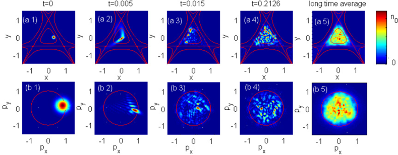
Figure 1: Time evolution of a wave-packet and the long-time average in the Henon-Heiles system. The first row is the density in the real space and the second row is the density in the momentum space. The long-time averages of these densities are shown at the rightmost panels. The average is taken over 1200 states equally separated in the time interval of $[0.2012,0.2255]$. The unit for the real space is $r_{c}$ and the unit for the momentum space is $p_{0}$. The red lines in the first row are energy contours of the Henon-Heiles potential at $V(x,y)/V_{c}=1/2,~{}1,~{}2$. The red lines in the second row are the maximal classically allowed momentum for the initial energy of the Gaussian wave packet. The color bars are given on the right side.

Equilibration of an isolated quantum chaotic system. The inequality proved for the quantum ergodic theorem by Reimann reimann_foundation_2008 was slightly modified by Short et al. short_equilibration_2011 ; short_quantum_2012 . This inequality for an observable $A$ now reads

$$\sigma^{2}_{A}\equiv\frac{\braket{}{\mbox{tr}\{A\rho(t)\}-\mbox{tr}(A\rho_{\infty})}{{}^{2}}_{t}}{\|A\|^{2}}\leq\frac{1}{d_{\mbox{eff}}}\,,$$ (1)

where $\rho(t)=\ket{\psi(t)}\bra{\psi(t)}$ with $\ket{\psi(t)}=\sum_{k}c_{k}\ket{E_{k}}$ being the wave function of the isolated system and $\rho_{\infty}=\sum_{k}|c_{k}|^{2}\ket{E_{k}}\bra{E_{k}}$. $\ket{E_{k}}$ is the energy eigenstate of the system. The subscript $t$ in $\braket{}_{t}$ represents an averaging over a time period much longer than the characteristic time scale of the system. $\|A\|^{2}$ is the maximal value of $A$ regarding all the states in the Hilbert space. The effective dimension $d_{\mbox{eff}}=\frac{1}{\sum_{k}(\mbox{tr}\ket{E_{k}}\bra{E_{k}}\rho(t))^{2}}$ indicates how widely the state $\ket{\Psi}$ is spread over the energy eigenstates. This inequality holds for a large class of quantum systems that satisfies the non-degenerate energy-gap conditionin eV ; reimann_foundation_2008 .

If a quantum system is in a typical state of high energy, then $d_{\mbox{eff}}$ should be large since the density of states usually increases tremendously with energy. This means that the right hand side of Eq.(1) is small. Therefore, this inequality tells us two things: (i) An isolated quantum system in a high-energy state will eventually relax to a state where an observable will fluctuate in small amplitude around its averaged value. (ii) Although the isolated quantum system is described by a wave function, the expectation value of any observable $A$ at almost any moment can be computed with $\rho_{\infty}$, that is, $\mbox{tr}(\rho A)\approx\mbox{tr}(\rho_{\infty}A)$.

Remarks are warranted here. (1) $\rho_{\infty}$ is different from the standard micro-canonical density matrix in textbooks huang_huang_1987 ; landau_landau_1958 : the coefficients $|c_{k}|^{2}$’s are determined by the initial condition and they are not necessarily equal to each other and distributed in a narrow energy range. (2) The coefficients $|c_{k}|^{2}$’s do not change with time; therefore, the energy distribution of the final equilibrated state is the same as the initial state.

For many physicists, small fluctuations already imply equilibrium; however, for others, a state is equilibrated only when its entropy is maximized. For the latter group, even though ground states and other eigenstates have no fluctuations, they can not be regarded as equilibrium. Von Neumann belongs to the latter group. By introducing an entropy for a pure state eV , he proved the quantum H-theorem , which demands that a low-entropy state evolve into a high-entropy state. We address this entropy issue with an example by defining a special entropy for pure states in the single particle Henon-Heiles system feit_wave_1984 . This is in spirit similar to the entropy for a pure state introduced by von Neumann, for which there is no known practical procedure to compute so far. Note that this entropy for a pure state introduced by von Neumann in 1929 is different from the usual von Neumann entropy, which is zero for all pure states.

We emphasize that it is reasonable to use a single-particle quantum chaotic system for illustration. When expressed in the form of matrix, there is no essential difference between one-body Hamiltonian and many-body Hamiltonian as long as they belong to the same class of random matrix gutzwiller_chaos_1990 . This is particularly true for the system’s energy spectrum, which appears to be the only factor in determining whether the system equilibrates or not eV ; reimann_foundation_2008 . We expect that the one-body and many-body systems share many dynamical features when their corresponding matrices belong to the same class. More discussion on this point can be found in Ref.zhuang2 .

The Hamiltonian of the system for the Henon-Heiles system is $H={p^{2}}/{2m}+\frac{\alpha}{2}(x^{2}+y^{2})+\lambda(x^{2}y-\frac{y^{3}}{3})$, which has three saddle points located at a distance $r_{c}\equiv\frac{\alpha}{\lambda}$ from the origin. These three points are the corners of the energy triangular contour with potential $V_{c}\equiv\frac{\alpha^{3}}{6\lambda^{2}}$ as shown in Fig.1(a1-a5). The momentum corresponding to the saddle point energy is $p_{0}\equiv\sqrt{2mV_{c}}$ as indicated by the circle in Fig.1(b1-b5). In our numerical simulation we set $m=\frac{1}{2}$, $\hbar=1$, and $\alpha/\lambda=1/3$.

The initial condition is a highly localized Gaussian wave packet as shown in Fig.1 (a1,b1) so that the system energy is high. This wave packet is centered at $\vec{r}_{i}=(0.3,0)r_{c}$ and $\vec{p}_{i}=(\cos 10^{\circ},\sin 10^{\circ})\sqrt{7/10}p_{0}$ in the real and momentum spaces, respectively. A classical particle with $\vec{r}_{i}$ and $\vec{p}_{i}$ has energy $0.9691V_{c}$ and its motion is fully chaotic.

We numerically solve the Schrödinger equation and the dynamical evolution of the wave packet is illustrated in Fig.1(a1-a4,b1-b4). As the wave packet evolves, it begins to spread out and distort in shape. Eventually it reaches an equilibrium state, where the wave packet spreads out all over the classically allowed region in the real space and the momentum space. This overall feature will no longer change even though the details of the wave packet still change in the following dynamical evolution. For comparison, we have calculated $n_{\infty}(\vec{r})=\braket{\vec{r}}{\rho_{\infty}}{\vec{r}}$ and $n_{\infty}(\vec{p})=\braket{\vec{p}}{\rho_{\infty}}{\vec{p}}$ by long-time averaging, i.e., the equilibrium state obtained by Reimann reimann_foundation_2008 . The results are shown in Fig.1(a5,b5). It is clear that $n_{\infty}(\vec{r})$ and $n_{\infty}(\vec{p})$ are very similar to the wave packet at $t=0.2126$ with the same overall feature that the wave function spread all over both the triangular spatial region and the circled momentum region except for some fluctuations.

To demonstrate the system has relaxed to an equilibrium state, we define an entropy as ${S_{\xi}}=-\int d\xi\frac{n(\xi,t)}{n_{\infty}(\xi)}\ln(\frac{n(\xi,t)}{n_{\infty}(\xi)}),\xi=\vec{r},~{}\vec{p}$. This entropy indicates how wide spread the wave function is in the classically-allowed region. The time evolution of ${S_{\xi}}$ is shown in Fig.2(a1,a2), where we see clearly the entropies quickly saturate and reach the maximum values, indicating that an equilibrium state is reached. Note that the relaxation times in both the real and momentum spaces are about the same. However, it must be pointed out that this definition of entropy applies only for some special systems and do not apply for a general quantum system. It is in spirit in accordance with the entropy for a pure state introduced for a general system by von Neumann eV .

The equilibrium state reached is consistent with the inequality Eq.(1). To check the inequality numerically, one needs to compute energy eigenstates of the system. As it is difficult to compute the eigenstates for the Henon-Heiles system, we have turned to the ripple billiard system studied in Ref.xiong_universal_2011 ; li_quantum_2002 to verify the inequality. The verification is successful and the detailed computation can found in Ref.zhuang2 . We only mention here that $d_{\rm eff}\approx 300$ for a similar Gaussian wave packet in the ripple billiard system.

Note that the quantum ergodic theorem was originally proved by von Neumann and Reimann for systems that have no degenerate energy gaps eV ; reimann_foundation_2008 . It was later generalized to systems that have limited amount of degeneracy  short_quantum_2012 . However, it is still not clear that how these degeneracy conditions are related to the integrability of the systems. Our numerical simulations here and elsewhere xiong_universal_2011 ; zhuang2 suggest that this theorem may be applied in a much broader class of quantum systems, which include quantum chaotic systems.

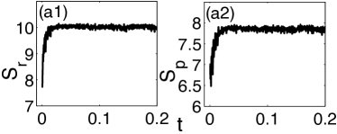
Figure 2: Time evolution of the entropies $S_{\xi}$ for the Henon-Heiles system for both spatial and momentum space.

Thermalization of subsystems. We have shown that a large class of truly isolated quantum systems, including chaotic systems, can relax to an equilibrium state. Now we decompose an equilibrated isolated quantum system into two parts, subsystem $S$ and thermal bath $B$. We consider an operator $\mbox{tr}^{(B)}$, which traces out the thermal bath $B$ and gives the density operator for the small subsystem $S$. Note the subsystem $S$ is small compared with system $S+B$ but still large on the microscopic level. Based on our equilibration picture, the expectation value of $\mbox{tr}^{(B)}$ should also equilibrate. We shall show that due to the coupling to the rest of the system, these equilibrated subsystems are also thermalized so that they are described by the Gibbs distribution. The derivation of Gibbs distribution for a subsystem has been considered before with the assumption that the isolated system is in a pure state composed of energy eigenstates from a small energy interval reimann_typicality_2007 ; riera_thermalization_2012 . We show that this assumption is not necessary and when the pure state is composed of energy eigenstates of different energy scales, the subsystem is thermalized with multiple temperatures.

We write the Hamiltonian of the isolated system as $H^{S+B}=H^{S}+H^{B}+\Delta H$, where $\Delta H$ is the weak interaction between system $H^{S}$ and thermal bath $H^{B}$. Suppose that the composite system is described by a wave function $\ket{\Phi^{S+B}}=\sum c_{k}\ket{E^{S+B}_{k}}$, where $\ket{E^{S+B}_{k}}$’s are the energy eigenstates of the composite system. By tracing out thermal bath $B$, we obtain the density operator for system $S$, $\rho^{S}=\mbox{tr}^{(B)}\ket{\Phi^{S+B}}\bra{\Phi^{S+B}}$. The system will eventually equilibrate; as an observable, $\rho^{S}$ will be close to its long time average, i.e. $\rho^{S}\approx\braket{\rho^{S}}_{t}\equiv\mbox{tr}^{(B)}\rho_{\infty}^{S+B}=\mbox{tr}^{(B)}\sum|c_{k}|^{2}\ket{E^{S+B}_{k}}\bra{E^{S+B}_{k}}$.

We expand the eigenstate $\ket{E^{S+B}_{k}}$ as follows

$$\ket{E_{k}^{S+B}}\approx{\sum}^{\prime}a_{ij}^{k}\ket{E^{S}_{i}}\ket{E^{B}_{j}}\,,$$ (2)

where $\ket{E^{S}_{i}}$ and $\ket{E^{B}_{j}}$ are energy eigenstates of system $S$ and thermal bath $B$, respectively. The prime above indicates that the summation is only over eigen-energies satisfying

$$E^{S+B}_{k}=E^{S}_{i}+E^{B}_{j}+\Delta E_{ij}\,.$$ (3)

where $\Delta E_{ij}$ is the interaction energy that is usually very small compared to $E^{S}_{i}$ and $E^{B}_{j}$ when long-range interaction is negligible, e.g., gravity, in the system. Two remarks are warranted. (i) The approximation made in Eq.(2) is justified. The equality holds when there is no coupling $\Delta H=0$. We expect it hold when the weak interaction $\Delta H$ is turned on. (ii) The weak interaction $\Delta H$ can drive the system to a state with $a^{k}_{ij}$’s randomly uniformly distributed on the sphere $\sum_{ij}|a^{k}_{ij}|^{2}=1$. This random distribution is similar to the idea of ”typicality” goldstein_canonical_2006 ; santos_weak_2012 . The connection between interaction and randomness is widely acknowledged since the details of the interaction is irrelevant to the statistical properties flambaum_towards_1996 ; borgonovi_chaos_1998 . As a result, the average value of $|a^{k}_{ij}|^{2}$ is $\frac{1}{D^{S+B}(E^{S+B}_{k})}$, where $D^{S+B}(E^{S+B}_{k})$ is the degeneracy brought by the combination of states. We emphasize that this degeneracy is different from the intrinsic degeneracy of the system and it is due to the existence of $\Delta E_{ij}$ in Eq.(3) .

With the approximation made in Eq.(2), we now proceed with our derivation,

$$\rho^{S} = \sum_{k}|c_{k}|^{2}\sum_{m}\braket{E_{m}^{B}}{E^{S+B}_{k}}\braket{E^{S+B}_{k}}{E_{m}^{B}}$$ (4)

$$= \sum_{k}|c_{k}|^{2}\sum_{ii^{\prime}}{}^{\prime}\{\sum_{m}a^{k}_{im}a^{k*}_{i^{\prime}m}\}\ket{E^{S}_{i}}\bra{E^{S}_{i^{\prime}}}$$

$$= \sum_{k}|c_{k}|^{2}\sum_{i}(\sum_{m}|a^{k}_{im}|^{2})\ket{E^{S}_{i}}\bra{E^{S}_{i}}$$

$$+\sum_{k}|c_{k}|^{2}\sum_{i\neq i^{\prime}}^{\prime}(\sum_{m}a^{k}_{im}a^{k*}_{i^{\prime}m})\ket{E^{S}_{i}}\bra{E^{S}_{i^{\prime}}}\,.$$

The central limit theorem gives the results of the first summation as $\sum_{m}|a^{k}_{im}|^{2}\simeq D^{B}(E^{B}_{m})/D^{S+B}(E^{S+B}_{k})$ and the second summation as $\sum_{m}a^{k}_{im}a^{k*}_{i^{\prime}m}\sim O\{\sqrt{D^{B}(E^{B}_{m})}/D^{S+B}(E^{S+B}_{k})\}\simeq O\{1/\sqrt{D^{S+B}(E^{S+B}_{k})}\}$ where $D^{B}(E^{B}_{m})$ is the degeneracy of the thermal bath and we have used that $S$ is much smaller than $B$ so that $D^{B}(E^{B}_{m})\simeq D^{S+B}(E^{S+B}_{k})$.

As a result, the last term in Eq.(4) has the order of magnitude at $O\{\sum_{i}{D^{S}(E_{i})}^{2}/\sqrt{D^{S+B}(E^{S+B}_{k})}\}$, which is practically zero for the isolated system is much larger than system $S$. So omitting the last term, we have from Eq.(4)

$$\rho^{S}=\sum_{k}|c_{k}|^{2}\sum_{i}\frac{D^{B}(E^{B}_{m})}{D^{S+B}(E^{S+B}_{k})}\ket{E^{S}_{i}}\bra{E^{S}_{i}}\,.$$ (5)

With the standard argument for the Gibbs distribution landau_landau_1958 , we arrive finally at

$$\rho^{S}=\sum_{k}|c_{k}|^{2}\{\sum_{i}\exp(-\beta_{k}E_{i})\ket{E^{S}_{i}}\bra{E^{S}_{i}}\}\,,$$ (6)

where $\beta_{k}\equiv\frac{1}{k_{B}T_{k}}\equiv{\partial\ln D^{S+B}(E^{S+B}_{k})}/{\partial E^{S+B}_{k}}$ defines the temperature of the total system for eigenstate $\ket{\Phi_{k}^{S+B}}$. In this way, we have proved that a subsystem of an isolated equilibrated system is thermalized.

Thermalized state with multiple temperatures. Here we examine Eq. (6) for two typical cases: (i) The coefficients $|c_{k}|^{2}$ of the composite system have a single sharp peak distribution around energy $E_{p}$. This case is considered by others  reimann_typicality_2007 in different formalisms. For this case, the density matrix $\rho^{S}$ in Eq.(6) is reduced to $\rho^{S}=\sum_{i}\exp(-\beta_{p}E_{i})\ket{\psi^{S}_{i}}\bra{\psi^{S}_{i}}$. This is exactly the typical Gibbs distribution discussed in all textbook on statistical mechanics. (ii) The coefficients $|c_{k}|^{2}$ have two well-separated sharp peaks around two energies $E_{p1}$ and $E_{p2}$. In other words, the composite system (or the heat bath) is in a superposition of numerous eigenstates centered around two very different energy scales. In this case, the thermalized system has two temperatures, $\beta_{1}$ for $E_{p1}$ and $\beta_{2}$ for $E_{p2}$, with the following density matrix

$$\rho^{S}=\sum_{i}(|a_{1}|^{2}e^{-\beta_{1}E_{i}}+|a_{2}|^{2}e^{-\beta_{2}E_{i}})\ket{E^{S}_{i}}\bra{E^{S}_{i}}\,,$$ (7)

where $|a_{1}|^{2}$ and $|a_{2}|^{2}$ are the weight of the two distribution peaks. The following is a list of key points for a good understanding of this quantum equilibrium state with two different temperatures.

1. When the quantum heat bath is in a superposition of states with two well-separated energy scales, each particle in the subsystem always feel different energy scales simultaneously when it exchanges energy with the heat bath. This leads to a thermalized state with two different temperatures.

2. When a system is in such a state, it consists of two parts, one hot and one cold. However, one can not tell which particle belongs to the hot part and which particle is in the cold part. This is similar to liquid helium. It consists of a superfluid part and a normal fluid part; but no single helium atom can be assigned to either the superfluid part or the normal fluid part.

3. When an ideal gas is thermalized to such an equilibrium state with two temperatures, each particle in the gas can be roughly viewed as in a superposition state of two different momenta. This is impossible in a classical ideal gas, where each particle has a definite momentum.

4. Since the total system $S+B$ is isolated, the coefficients $|c_{k}|^{2}$s are constants of motion and only depend on the initial condition. As a result, the two peaks in the initial distribution of $|c_{k}|^{2}$’s will remain intact during the whole dynamical process. In other words, the system is stable with the double-peak energy distribution.

5. If the total system $S+B$ is a superposition of just two different energy eigenstates, the total system is not in an equilibrium state. This is because in this case $d_{\rm eft}=2$ and the left hand side of the inequality is large. To ensure equilibration, we need $d_{\rm eft}\gg 1$, that is to have large number of eigenstates concentrating around two different energy scales.

6. This state does not describe a statistical ensemble of systems, where some systems are cold and some systems are hot.

7. Our state is an equilibrium state with multiple temperatures; it is completely different from the usual non-equilibrium state which has different temperatures for different parts.

8. Our state is not a Schrödinger cat state Cat ; it does not collapse upon measurement.

For most of the systems that we have encountered in nature or studied in experiment, they are in contact with classical heat bath. However, with the advance of technology, we can now create large quantum systems which can serve as quantum heat bath. Two such examples are Bose-Einstein condensates (BECs) and nuclear spins in a quantum dot, where feasible experiments can be set up to test our prediction. (i) Consider a two-species BEC. One species with larger population is trapped optically in an uneven double-well potential shin_distillation_2004 while the smaller species is trapped in a single well potential. The larger species serves as a heat bath with two energy peaks due to uneven double-well potential. By exchanging energy with the larger species, the smaller species should develop a double-peak distribution in momentum space, signaling the existence of two temperatures. Since the uneven double-well has to be kept for the double-peaked energy distribution, the state realized here is not strictly equilibrium and might be more accurately called stationary. Now a two-species BEC has been realized just recently in experiment wangdj (ii) Due to the weak coupling to the enviornment, nuclear spins in a quantum dot can be regarded as quantum bath for a long time yao_prb_2006 ; zhao_anomalous_2011 ; huang_observation_2011 . With the feedback technique that has been demonstrated both theoretically and experimentally yao_nature , one should be readily design a scheme that can put these nuclear spins in a superposition state of two different energy scales and use the electron spin to probe such a state yao_private .

Note that Fine et al. have also abandoned the transitional microcanonical ensemble and replaced it with “quantum microcanonical” ensemble Fine3 ; Fine2 ; Fine1 . This is fundamentally different from our approach, where no assumption for an ensemble is needed.

- (1) K. Huang, Statistical Mechanics, page 176. John Wiley & Sons, Inc., 2 edition (1987).
- (2) L. Landau and E. Lifshitz, Statistical Physics, pages 78–80. Pergamon, London(1958).
- (3) J. von Neumann, Z. Phys. 57, 30 (1929); [Eur. Phys. J. H 35, 201 (2010)].
- (4) S. Goldstein, J. L. Lebowitz, R. Tumulka, and N. Zanghi European Phys. J. H 35, 173 (2010).
- (5) J.L. Lebowitz, Phys. Today, 46(9), 32 (1993).
- (6) J. Gemmer, M. Michel, and G. Mahler, Quantum Thermodynamics, Lecture Notes in Physics, pages 86–126. Springer–Verlag Berlin Heidelberg, 2 edition (2009).
- (7) J.M. Deutsch, Phys. Rev. A, 43, 2046 (1991).
- (8) M. Srednicki, Phys. Rev. E, 50, 888 (1994).
- (9) P. Reimann, Phys. Rev. Lett., 101, 190403 (2008).
- (10) M. Rigol, V. Dunjko, and M. Olshanii, Nature, 452, 854 (2008).
- (11) G. Biroli, C. Kollath, and A.M. Läuchli, Phys. Rev. Lett., 105, 250401 (2010).
- (12) A.C. Cassidy, C.W. Clark, and M. Rigol, Phys. Rev. Lett., 106, 140405 (2011).
- (13) M. Rigol and M. Srednicki, Phys. Rev. Lett., 108, 110601 (2012).
- (14) A.J. Short, New J. Phys., 13(5), 053009 (2011).
- (15) A.J. Short and T.C. Farrelly, New J. Phys., 14, 013063 (2012).
- (16) S. Popescu, A.J. Short, and A. Winter, Nature Phys., 2, 754 (2006).
- (17) S. Popescu, A.J. Short, and A. Winter, arXiv:quant-ph/0511225 (2005).
- (18) H. Dong, S. Yang, X. F. Liu, and C. P. Sun, Phys. Rev. A 76, 044104 (2007).
- (19) W. Wang, Phys. Rev. E 86, 011115 (2012).
- (20) N. Linden, S. Popescu, A.J. Short, and A. Winter, Phys. Rev. E, 79, 061103 (2009).
- (21) J. Cho and M.S. Kim, Phys. Rev. Lett., 104, 170402 (2010).
- (22) T.N. Ikeda, Y. Watanabe, and M. Ueda, Phys. Rev. E, 84, 021130 (2011).
- (23) M. Rigol, V. Dunjko, V. Yurovsky, and M. Olshanii, Phys. Rev. Lett., 98, 050405 (2007).
- (24) P. Reimann and M. Kastner, New J. Phys., 14, 043020 (2012).
- (25) H. Xiong and B. Wu, Laser Phys. Lett., 8, 398 (2011).
- (26) S. Goldstein, J.L. Lebowitz, R. Tumulka, and N. Zanghí, Phys. Rev. Lett., 96, 050403 (2006).
- (27) L.F. Santos, A. Polkovnikov, and M. Rigol, Phys. Rev. E, 86, 010102 (2012).
- (28) P. Reimann, Phys. Rev. Lett., 99, 160404 (2007).
- (29) V.I. Yukalov, Laser Phys. Lett., 8, 485 (2011).
- (30) V.I. Yukalov, Ann. Phys., 327, 253 (2012).
- (31) V.I. Yukalov, Phys. Lett. A, 375, 2797 (2011).
- (32) A. Riera, C. Gogolin, and J. Eisert, Phys. Rev. Lett., 108, 080402 (2012).
- (33) C. Gogolin, M.P. Müller, and J. Eisert, Phys. Rev. Lett., 106(4), 040401 (2011).
- (34) C. Gogolin, arXiv:quant-ph/1003.5058 (2010).
- (35) S. Sugiura and A. Shimizu, Phys. Rev. Lett., 108, 240401 (2012); S. Sugiura and A. Shimizu Phys. Rev. Lett. 111, 010401 (2013).
- (36) C. Ududec, N. Wiebe, and J. Emerson, Phys. Rev. Lett. 111, 080403 (2013); S. Goldstein, T. Hara, and H. Tasaki Phys. Rev. Lett. 111, 140401 (2013).
- (37) T. Kinoshita, T. Wenger, and D.S. Weiss, Nature, 440, 900 (2006).
- (38) H-J Stöckmann, Quantum Chaos, an introduction, Chapter 2, Cambridge University Press (1999).
- (39) M.V. Berry, J. Phys. A: Math. Gen., 10, 2083 (1977).
- (40) M.V. Berry, Phil. Trans. R. Soc. A, 287, 237 (1977).
- (41) M.D. Feit and J.A. Fleck, J. Chem. Phys., 80, 2578 (1984); R. A. Pullen and A. R. Edmonds, J. Phys. A: Math. Gen. 14 L477 (1981); D Engel, J Main, and G Wunner, J. Phys. A: Math. Gen. 31 (1998) 6965; M. Brack, R. K. Bhaduri, J. Law, and M. V. N. Murthy, Phys. Rev. Lett. 70, 568 (1993); D. W. Noid and R. A. Marcus, J. Chem. Phys. 67, 559 (1977).
- (42) Q. Zhuang and B. Wu, arXiv:1308.1717 (2013).
- (43) W. Li, L.E. Reichl, and B. Wu, Phys. Rev. E, 65, 056220 (2002).
- (44) V.V. Flambaum, F.M. Izrailev, and G. Casati, Phys. Rev. E, 54, 2136 (1996).
- (45) F. Borgonovi, I. Guarneri, F. Izrailev, and G. Casati, Phys. Lett. A, 247, 140 (1998).
- (46) Y. Shin et al., Phys. Rev. Lett., 92, 150401 (2004).
- (47) A.J. Leggett, Science, 307, 871 (2005).
- (48) Dezhi Xiong, Xiaoke Li, Fudong Wang, and Dajun Wang, arXiv:1305.7091 (2013).
- (49) W. Yao, R.B. Liu, L.J. Sham, Phys. Rev. B, 74, 195301 (2006).
- (50) N. Zhao, Z.Y. Wang, and R.B. Liu, Phys. Rev. Lett., 106, 217205 (2011).
- (51) P. Huang et al., Nature Commu., 2, 570 (2011).
- (52) X.-D. Xu et al., Nature, 459, 1105 (2009); W. Yao and Y. Luo, EPL, 92 (2010) 17008.
- (53) Wang Yao, private communication.
- (54) K. Ji and B.V. Fine, Phys. Rev. Lett., 107, 050401 (2011).
- (55) B.V. Fine and F. Hantschel, arXiv:cond-mat/1010.4673 (2010).
- (56) B.V. Fine, Phys. Rev. E, 80, 051130 (2009).