Gate control of Berry phase in III-V semiconductor quantum dots

Abstract

We analyze the Berry phase in III-V semiconductor quantum dots (QDs). We show that the Berry phase is highly sensitive to electric fields arising from the interplay between the Rashba and Dresselhaus spin-orbit (SO) couplings. We report that the accumulated Berry phase can be induced from other available quantum states that differ only by one quantum number of the corresponding spin state. The sign change in the $g$-factor due to the penetration of Bloch wavefunctions into the barrier materials can be reflected in the Berry phase. We provide characteristics of the Berry phase for three different length scales (spin-orbit length, hybrid orbital length and orbital radius). We solve the time dependent Schr$\mathrm{\ddot{o}}$dinger equation by utilizing the Feynman disentangling technique, and we investigate the evolution of spin dynamics during the adiabatic transport of QDs in the two-dimensional plane. Our results can pave the way to building a topological quantum computer in which the Berry phase can be engineered and be manipulated with the application of the spin-orbit couplings through gate-controlled electric fields.

I Introduction

Coherent control of single-electron spin relaxation and its measurement in III-V semiconductor quantum dots might provide a new foundation of architecture to build next-generation spintronic devices. Amasha et al. (2008); Takahashi et al. (2010); Prabhakar et al. (2013); Awschalom et al. (2002); Loss and DiVincenzo (1998); Prabhakar and Raynolds (2009); Prabhakar et al. (2011) To manipulate the spin in quantum dots (QDs), achieving the state of the art of semiconductor technology, a number of researchers have recently proposed measuring spin behavior in QDs by utilizing electric fields generated by isotropic and anisotropic gate potentials. Amasha et al. (2008); Takahashi et al. (2010); de Sousa and Das Sarma (2003); Prabhakar and Raynolds (2009); Prabhakar et al. (2011, 2012) The effective $g$-factor and phonon mediated spin relaxation in both isotropic and anisotropic QDs can be tuned with spin-orbit coupling. de Sousa and Das Sarma (2003); Takahashi et al. (2010); Prabhakar et al. (2012) The electric-field control of spin provides an opportunity for tuning the spin current on and off in QDs formed in a single electron transistor. Such control can help to initialize the electron spin in spintronic devices. Amasha et al. (2008); Takahashi et al. (2010); Bandyopadhyay (2000); Flatté (2011)

Alternatively, a more robust technique can be applied to manipulate single electron spins in QDs through the non-Abelean geometric phases. Giuliano et al. (2003); Aleiner and Fal’ko (2001); Wang and Zhu (2008); Yang and Hwang (2006); Eric Yang (2006); Yang (2007); Berry (1984) For a system of degenerate quantum states, Wilczek and Zee showed that the geometric phase factor is replaced by a non-Abelian time dependent unitary operator acting on the initial states within the subspace of degeneracy. Wilczek and Zee (1984); Prabhakar et al. (2010) Since then, the geometric phase has been measured experimentally for a variety of systems, such as quantum states driven by a microwave field Pechal et al. (2012) and qubits with tilted magnetic fields. Berger et al. (2012); Leek et al. (2007) Manipulation of spin qubits through the Berry phase implies that injected data can be read out with a different phase that is topologically protected from the outside world. Das Sarma et al. (2005); Hu and Das Sarma (2000); Loss et al. (1990); Tserkovnyak and Loss (2011); San-Jose et al. (2006, 2008, 2007); Jones et al. (2000); Falci et al. (2000) Several recent reviews of the Berry phase have been presented in Refs. Xiao et al., 2010; Nayak et al., 2008. One of the promising research proposals for building a solid-state topological quantum computer is that the accumulated Berry phase in a QD system may be manipulated using the interplay between the Rashba-Dresselhaus spin-orbit couplings. San-Jose et al. (2006); Aleiner and Fal’ko (2001) The Rashba spin-orbit coupling arises from the asymmetric triangular quantum well along the growth direction, while the Dresselhaus spin-orbit coupling arises due to bulk inversion asymmetry in the crystal lattice. Bychkov and Rashba (1984); Dresselhaus (1955) A recent work by Bason et al. shows that the Berry phase can be measured for a two level quantum system in a superadiabatic basis comprising the Bose-Einstein condensates in optical lattices. Bason et al. (2012)

Recently, it has also been shown that the geometric phase can be induced on the electron spin states in QDs by moving the dots adiabatically in a closed loop in the two dimensional ($2$D) plane plane through application of a gate controlled electric field. Prabhakar et al. (2010); San-Jose et al. (2008); Ban et al. (2012); Prabhakar et al. (2014) Furthermore, the authors in Refs. Bednarek et al., 2012, 2008; Bednarek and Szafran, 2008 have recently proposed building a QD device in the absence of magnetic fields that can perform quantum gate operations (NOT gate, Hadamard gate and Phase gate) using an externally applied sinusoidal varying potential through external gates.

In this paper, we show how to transport electron spin states of QDs in the presence of externally applied magnetic fields along the z-direction in a closed loop through the application of a time dependent distortion potential. We investigate the interplay between the Rashba and the Dreeselhaus spin-orbit couplings on the scalar Berry phase. Yang and Hwang (2006); Wu et al. (2011) The transport of the dots is carried out very slowly, so that the adiabatic theorem can be applied on the evolution of the spin dynamics. In particular, the sign change in the $g$-factor of electrons in the QDs due to the penetration of the Bloch wavefunctions into the barrier materials can be manipulated with the interplay between the Rashba-Dresselhaus spin-orbit couplings in the Berry phase. We show that the Berry phase in QDs can be engineered and therefore manipulated with the application of spin-orbit couplings through gate controlled electric fields. We solve the time dependent Schr$\mathrm{\ddot{o}}$dinger equation and investigate the evolution of spin dynamics in QDs.

The paper is organized as follows. In Sec. II, we provide a detailed theoretical formulation of the total Hamiltonian of a moving QD in relative coordinates and relative momentum. We also show that the quasi adiabatic variables are gauged away from the total Hamiltonian. Here we write the total Hamiltonian of the moving dots in terms of annihilation and creation operators and we utilize the perturbation theory to find the analytical expression of the Berry phase. In Sec. III, we provide details of our computational methodology. In Sec. IV, we investigate the interplay between the Rashba-Dresselhaus spin-orbit couplings on the Berry phase of III-V semiconductor QDs. Finally, in Sec. V, we summarize our results.

II Theoretical Model

We consider the Hamiltonian $H=H_{0}+H_{so}$ for an electron in a QD of the III-V semiconductor. Prabhakar and Raynolds (2009); Prabhakar et al. (2011) Here

$$H_{0}={\frac{\left\{\mathbf{p}+e\mathbf{A}(\mathbf{r})\right\}^{2}}{2m}}+{\frac{1}{2}}m\omega_{o}^{2}\mathbf{r}^{2}+e\mathbf{E}(t)\cdot\mathbf{r}+\frac{g_{0}\mu B\sigma_{z}}{2}$$ (1)

is the Hamiltonian for a QD electron in the x-y plane of the two-dimensional electron gas (2DEG) in the presence of a uniform magnetic field B along the z-direction and a time dependent lateral electric field $\mathbf{E}(t)$. The second term is the spin-orbit Hamiltonian consisting of the Rashba and the linear Dresselhaus couplings, $H_{so}=H_{R}+H_{D}$, where

$$H_{R}=\frac{\alpha_{R}}{\hbar}\left\{\sigma_{x}\left(p_{y}+eA_{y}\right)-\sigma_{y}\left(p_{x}+eA_{x}\right)\right\},$$ (2)

$$H_{D}=\frac{\alpha_{D}}{\hbar}\left\{-\sigma_{x}\left(p_{x}+eA_{x}\right)+\sigma_{y}\left(p_{y}+eA_{y}\right)\right\},$$ (3)

with $\alpha_{R}=\gamma_{R}eE_{z}$ and $\alpha_{D}=0.78\gamma_{D}\left(2me/\hbar^{2}\right)^{2/3}E_{z}^{2/3}$.

In (1), $\mathbf{r}=\left(x,y,0\right)$ is the position vector and $\mathbf{p}=-i\hbar(\partial_{x},\partial_{y},0)$ is the canonical momentum. The vector potential $\mathbf{A}(\mathbf{r})$ is due to the applied magnetic field $\mathbf{B}$. Here $-e<0$ is the electronic charge, $m$ is the effective mass of an electron and $\mu$ is the Bohr magneton. The confining potential is parabolic with the center at $\mathbf{r}=0$. The third term in (1) is the electric potential energy due to an applied periodic lateral electric field $\mathbf{E}(t)=\left(E_{x}(t),E_{y}(t),0\right)$, where $E_{x}(t)=E_{0}\cos\omega t$ and $E_{y}(t)=E_{0}\sin\omega t$. Varying $\mathbf{E}(t)$ very slowly, we treat its two components as adiabatic parameters. In principle, the alternating electric field induces a vector potential added to the one due to the applied uniform magnetic field $\mathbf{B}$ in the z-direction. However, such a contribution to $\mathbf{B}$ is in practice extremely small as reported earlier by Golovach et. al. Golovach et al. (2006) Our estimate shows that by using the dot size $\ell_{0}=20~{}\mathrm{nm}$, the orbital radius $r_{0}\approx 70\mathrm{nm}$, the frequency $\omega=1~{}\mathrm{THz}$, and the maximum electric field $E_{0}=0.5~{}\mathrm{mV/nm}$, the magnitude of the induced magnetic field is approximately $B_{in}\approx\epsilon_{r}\mu_{r}\pi r_{0}\omega E_{0}/(2c^{2})\approx\epsilon_{r}\mu_{r}\times 10^{-6}~{}tesla$, where $\epsilon_{r}$ and $\mu_{r}$ are the relative electric permittivity and the magnetic permeability, respectively (for mathematical derivation, see appendix A). This contribution is negligible compared to the applied $\mathrm{\mathbf{B}}$ field. Therefore, for the vector potential, we simply choose the gauge of the form $A(r)=B/2\left(-y,x,0\right)$. The last term of (1) describes the Zeeman coupling with $g_{0}$, the bulk $g$-factor. Saniz et. al. Saniz et al. (2003) have suggested that the Coulomb repulsion between electrons with opposite spins of strongly correlated systems would give rise to appreciable oscillations in spin polarization. For weakly correlated systems, such effect vanishes. Hence, the Berry phase in QDs, for strongly correlated systems, is also influenced by Coulomb repulsion. As is pointed out by Saniz et. al., Saniz et al. (2003) the Coulomb coupling becomes weaker with decreasing electron density and increasing dot size. Since the dot size of our choice is $\ell_{0}=20~{}\mathrm{nm}$, the Coulomb coupling is very small as compared with the Zeeman coupling. Thus, in our model, the Coulomb coupling is not included. For strongly correlated systems with $\ell_{0}=0.5~{}\mathrm{nm}$ or less, the Coulomb coupling can not be ignored.

The electric field at a fixed time $t_{0}$ effectively shifts the center of the parabolic potential from $\mathbf{r}=0$ to $\mathbf{r}=\mathbf{r_{0}}\left(t_{0}\right)$, where $\mathbf{r}_{0}=-e\mathbf{E}\left(t_{0}\right)/m\omega_{0}^{2}$. Hence the Hamiltonian (1) can be expressed as

$$H_{0}={\frac{\left\{\mathbf{p}+e\mathbf{A}(\mathbf{r})\right\}^{2}}{2m}}+{\frac{1}{2}}m\omega_{o}^{2}\left(\mathbf{r}-\mathbf{r_{0}}\right)^{2}-G+{\frac{\Delta}{2}}\sigma_{z},$$ (4)

where $G=e^{2}E_{0}^{2}/\left(2m\omega^{2}_{0}\right)$ is an unimportant constant and $\Delta=g_{0}\mu B$ is the Zeeman energy. As the applied $\mathbf{E}-$field varies, the QD will be adiabatically transported along a circle of radius $r_{0}=|\mathbf{r}_{0}|=eE_{0}/m\omega^{2}_{0}$.

At this point, we introduce the relative coordinate $\mathbf{R}=\mathbf{r}-\mathbf{r_{0}}=\left(X,Y,0\right)$ and the relative momentum $\mathbf{P}=\mathbf{p}-\mathbf{p_{0}}=\left(P_{X},P_{Y},0\right)$, where $\mathbf{p_{0}}$ is the momentum of the slowly moving dot which may be classically given by $m\mathbf{\dot{r}}_{0}$. Obviously $\left[X,P_{X}\right]=\left[Y,P_{Y}\right]=i\hbar$ and $\left[X,P_{Y}\right]=\left[Y,P_{X}\right]=0$. We can show that the adiabatic variables $\mathbf{p}_{0}$ and $\mathbf{r}_{0}$ will be gauged away from the Hamiltonian by the transformation $\tilde{H}=UHU^{-1}$ and $\tilde{\psi}=U\psi$ with $U=\exp\left\{\left(i/\hbar\right)\left(\mathbf{p_{0}}+e\mathbf{A}\left(\mathbf{r}_{0}\right)\right)\cdot\mathbf{R}\right\}$, so that

$$\tilde{H}_{0}={\frac{1}{2m}}\left\{\mathbf{P}+e\mathbf{A}(\mathbf{R})\right\}^{2}+{\frac{1}{2}}m\omega_{o}^{2}R^{2}-G+{\frac{\Delta}{2}}\sigma_{z},$$ (5)

$$\tilde{H}_{so}=UH_{so}\left(\mathbf{p},\mathbf{r}\right)U^{-1}=H_{so}\left(\mathbf{P},\mathbf{R}\right),$$ (6)

where $\mathbf{A}\left(\mathbf{P},\mathbf{R}\right)=\left(B/2\right)\left(-Y,X,0\right)$. This means that the electron in the shifted dot obeys a quasi-static eigenequation, $\tilde{H}\left(\mathbf{P},\mathbf{R}\right)\tilde{\psi}_{n}\left(\mathbf{R}\right)=\tilde{\varepsilon}_{n}\tilde{\psi}_{n}\left(\mathbf{R}\right)$, where $\tilde{H}=\tilde{H}_{0}+\tilde{H}_{so}$. By an adiabatic transport of the dot, the eigenfunction $\tilde{\psi}_{n}$ will acquire the Berry phase as well as the usual dynamical phase. Namely, $\psi_{n}\left(\mathbf{r},t\right)=e^{i\gamma_{n}\left(t\right)}e^{i\theta_{n}\left(t\right)}U^{-1}\tilde{\psi}_{n}\left(R\right)$, where $\gamma_{n}$ is the Berry phase and $\theta_{n}$ is the dynamical phase.

In order to evaluate the Berry phase explicitly, we return to the original Hamiltonian $H$ and put it in the form:

$$H=\tilde{H}_{0}\left(\mathbf{P},\mathbf{R}\right)+H_{so}\left(\mathbf{P},\mathbf{R}\right)+H_{ad}\left(\mathbf{P},\mathbf{R};\mathbf{p_{0}},\mathbf{r_{0}}\right),$$ (7)

where

$$H_{ad}\left(\mathbf{P},\mathbf{R};\mathbf{p}_{0},\mathbf{r}_{0}\right) = \frac{1}{m}\left\{\mathbf{P}+e\mathbf{A}\left(\mathbf{R}\right)\right\}\cdot\left\{\mathbf{P}+e\mathbf{A}\left(\mathbf{R}\right)\right\}$$ (8)

$$+H_{so}\left(\mathbf{p}_{0},\mathbf{r}_{0}\right)+G^{\prime},$$

with another unimportant constant $G^{\prime}=\left\{\mathbf{p}_{0}+e\mathbf{A}\left(\mathbf{r}_{0}\right)\right\}^{2}/\left(2m\right)^{2}=\left(\omega+\omega_{c}/2\right)^{2}r_{0}^{2}/4$.

The quasi-static Hamiltonian $\tilde{H}_{0}\left(\mathbf{P},\mathbf{R}\right)$ can be diagonalized on the basis of the number states $|n_{+},n_{-},\pm 1\rangle$:

$$\tilde{H}_{0}=\left(N_{+}+\frac{1}{2}\right)\hbar\Omega_{+}+\left(N_{-}+\frac{1}{2}\right)\hbar\Omega_{-}-G+\frac{\Delta}{2}\sigma_{z},$$ (9)

where $N_{\pm}=a^{\dagger}_{\pm}a_{\pm}$ are the number operators with eigenvalues $n_{\pm}\in N_{0}$. Here,

$$a_{\pm}=\frac{1}{\sqrt{4m\hbar\Omega}}\left(iP_{x}\pm P_{y}\right)+\sqrt{\frac{m\Omega}{4\hbar}}\left(X\mp iY\right),$$ (10)

$$a_{\pm}^{\dagger}=\frac{1}{\sqrt{4m\hbar\Omega}}\left(-iP_{x}\pm P_{y}\right)+\sqrt{\frac{m\Omega}{4\hbar}}\left(X\pm iY\right),$$ (11)

provided that $\left[a_{\pm},a_{\pm}^{\dagger}\right]=1$. Correspondingly, the other terms may also be expressed in terms of the raising and lowering operators,

$$H_{so}\left(\mathbf{P},\mathbf{R}\right) = \alpha_{R}\left(\xi_{+}\sigma_{+}a_{+}-\xi_{-}\sigma_{-}a_{-}\right)~{}~{}~{}~{}~{}~{}$$ (12)

$$+i\alpha_{D}\left(\xi_{+}\sigma_{-}a_{+}+\xi_{-}\sigma_{+}a_{-}\right)+H.c.,~{}~{}~{}~{}~{}~{}$$

$$H_{ad} = \frac{\hbar}{2}\left(\xi_{+}z_{+}a_{+}-\xi_{-}z_{-}a_{-}\right)\omega_{+}$$ (13)

$$+\frac{1}{\hbar}\left(\alpha_{R}z_{-}-i\alpha_{D}z_{+}\right)m\omega_{+}\sigma_{+}+H.c.$$

In the above, we have used the notations, $z_{\pm}=x_{0}\pm iy_{0}$, $\xi_{\pm}=\sqrt{m\Omega/\hbar}\pm eB/\sqrt{4m\hbar\Omega}$, $\sigma_{\pm}=\left(\sigma_{x}\pm i\sigma_{y}\right)/2$, $\omega_{\pm}=\omega\left(1\pm\omega_{c}/\left(2\omega\right)\right)$, $\Omega_{\pm}=\Omega\pm\omega_{c}/2$ and $\Omega=\sqrt{\omega_{0}^{2}+\omega_{c}^{2}/4}$ with $\omega_{c}=eB/m$ being the cyclotron frequency. In (12) and (13), $H.c.$ signifies the Hermitian conjugate.

For III-V semiconductor QDs, we define the SO lengths $\lambda_{R}=\hbar^{2}/m\alpha_{R}$ and $\lambda_{D}=\hbar^{2}/m\alpha_{D}$ and estimate that the SO lengths are much larger than the hybrid orbital length $\ell$ and QDs radius $\ell_{0}$ (see left panel of Fig. 5). Therefore the Rashba-Dresselhaus SO couplings Hamiltonians are considered as a small perturbations. Based on the second order perturbation theory, the four lowest energy eigenvalues of the moving dot are given by

$$\varepsilon_{0,0,-1}=\hbar\Omega-G-\frac{\Delta}{2}-\frac{\alpha_{R}^{2}\xi_{-}^{2}}{\hbar\left(\Omega-\omega_{c}/2\right)+\Delta}-\frac{\alpha_{D}^{2}\xi_{+}^{2}}{\hbar\left(\Omega+\omega_{c}/2\right)+\Delta}+\varepsilon^{(2)}_{0,0,-1},~{}~{}~{}~{}~{}~{}$$ (14)

$$\varepsilon_{0,0,1}=\hbar\Omega-G+\frac{\Delta}{2}-\frac{\alpha_{R}^{2}\xi_{+}^{2}}{\hbar\left(\Omega+\omega_{c}/2\right)-\Delta}-\frac{\alpha_{D}^{2}\xi_{-}^{2}}{\hbar\left(\Omega-\omega_{c}/2\right)-\Delta}+\varepsilon^{(2)}_{0,0,1},~{}~{}~{}~{}~{}~{}$$ (15)

$$\varepsilon_{0,1,-1}=\frac{1}{2}\hbar\left(\Omega_{+}+3\Omega_{-}\right)-G-\frac{\Delta}{2}-\frac{2\alpha_{R}^{2}\xi_{-}^{2}}{\hbar\left(\Omega-\omega_{c}/2\right)+\Delta}-\frac{\alpha_{D}^{2}\xi_{+}^{2}}{\hbar\left(\Omega+\omega_{c}/2\right)+\Delta}+\frac{\alpha_{D}^{2}\xi_{-}^{2}}{\hbar\left(\Omega-\omega_{c}/2\right)-\Delta}+\varepsilon^{(2)}_{0,1,-1},~{}~{}~{}~{}~{}$$ (16)

$$\varepsilon_{0,1,1}=\frac{1}{2}\hbar\left(\Omega_{+}+3\Omega_{-}\right)-G+\frac{\Delta}{2}-\frac{2\alpha_{D}^{2}\xi_{-}^{2}}{\hbar\left(\Omega-\omega_{c}/2\right)-\Delta}+\frac{\alpha_{R}^{2}\xi_{-}^{2}}{\hbar\left(\Omega-\omega_{c}/2\right)+\Delta}-\frac{\alpha_{R}^{2}\xi_{+}^{2}}{\hbar\left(\Omega+\omega_{c}/2\right)-\Delta}+\varepsilon^{(2)}_{0,1,1},~{}~{}~{}~{}~{}$$ (17)

where

$$\varepsilon^{(2)}_{00\pm 1} = \pm\left(\frac{m\omega_{+}}{\hbar\sqrt{\Delta}}\right)^{2}\{(\alpha^{2}_{R}+\alpha^{2}_{D})r_{0}^{2}-4\alpha_{R}\alpha_{D}x_{0}y_{0}\}$$ (18)

$$-\left(\frac{\hbar\omega^{2}_{+}}{4}\right)\left\{\frac{\xi^{2}_{-}}{\Omega_{-}}+\frac{\xi^{2}_{+}}{\Omega_{+}}\right\}r_{0}^{2}=\varepsilon^{(2)}_{01\pm 1}.$$

Since $x_{0}y_{0}=r_{0}^{2}\sin 2\theta/2$, we conclude that the energy spectrum of the dot depends on the rotation angle. As a result, it is possible to have the interplay between the spin-orbit coupling and the evolution of spin dynamics during the adiabatic transport of the dots (see Fig. 2). In the above equation, we see that $\varepsilon^{(2)}_{00\pm 1}=\varepsilon^{(2)}_{01\pm 1}$. This means that the Berry phase depends not on how quantum states of the dot traveled but only on the total adiabatic area enclosed during the adiabatic transport of the dot in the 2D plane.

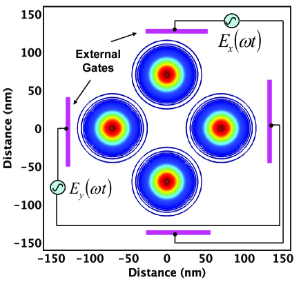
Figure 1: (Color online) Contour plots of the realistic electron wave functions in GaAs QDs that are adiabatically transported in one complete rotation in the plane of 2DEG under the influence of externally applied gate potential. We chose $E_{0}=5\times 10^{3}$ V/cm, $E_{z}=5\times 10^{5}$V/cm, $B=1$T and $\ell_{0}=20$nm. Here we report that $\varepsilon_{0,1,+1}-\varepsilon_{0,0,+1}\approx 2.1$ meV which is constant during the adiabatic transport of the QDs.

Figure 2: (Color online) Evolution of spin dynamics during the adiabatic transport of the GaAs QDs (see appendix B). The parameters are chosen the same as in Fig. 1 but $\ell_{0}=30$nm.

Figure 3: Components of the evolution operator  (see Eq. 38 in Appendix B) vs rotation angle. The parameters are chosen the same as in Fig. 2. Superposition of these components of the evolution operator induces spin-echo in the expectation values of the Pauli spin matrices in Fig. 2 during the adiabatic transport of the QDs in the plane of 2DEG.

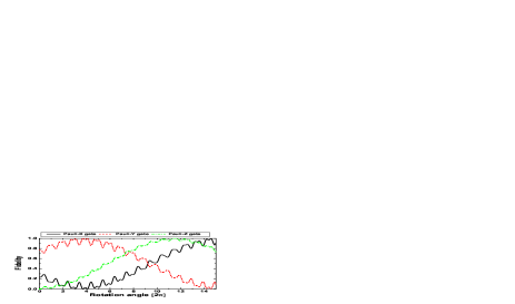
Figure 4: Evolution of three Pauli gate fidelities during the adiabatic transport of the dots in the 2D plane. Here the measurement of the gate fidelity is expressed in terms of the probability between the objective or ideal vector state and the evolution of spin dynamics along the circular trajectory (see the text for details). The parameters are chosen the same as in Fig. 1, but $\ell_{0}=15$nm.

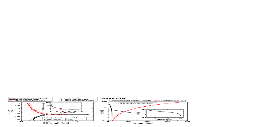
Figure 5: (Color online) (left panel) The Berry phase vs SO lengths on spin state $|0,0,+1\rangle$. Here we chose $\ell_{0}=20~{}\mathrm{nm}$. (right panel) The Berry phase vs hybrid orbital length and orbital radius on spin state $|0,0,+1\rangle$. Here we chose $\ell_{0}=20~{}\mathrm{nm}$ for solid line and $B=1~{}\mathrm{T}$ for dashed dotted line. The parameters are chosen the same as in Fig. 1.

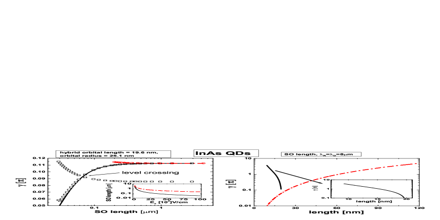
Figure 6: (Color online) See caption to Fig. 5 (it is the same, but for InAs QDs).

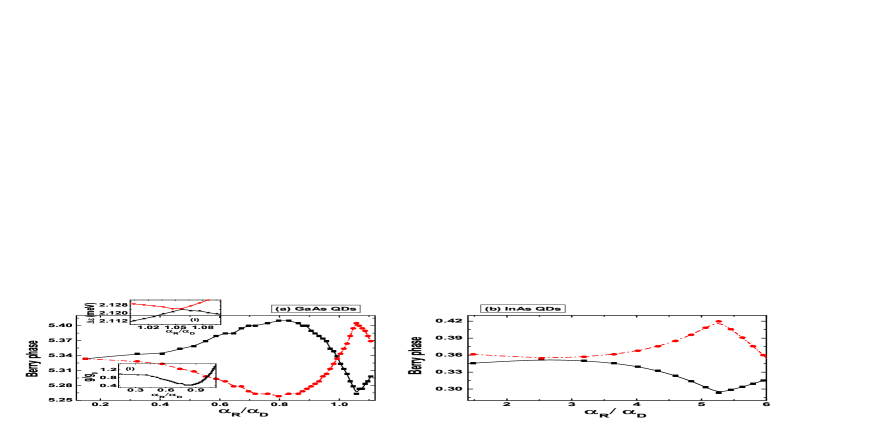
Figure 7: (Color online) The Berry phase (absolute value) on the spin state $|0,0,+1\rangle$ (solid lines, filled circles) and $|0,0,-1\rangle$ (dashed-dotted line, open circles) vs $\alpha_{R}/\alpha_{D}$ in QDs. Inset plot (i) shows the energy difference ($\varepsilon_{0,1,+1}-\varepsilon_{0,0,-1}$ (triangle pointing down)) and ($\varepsilon_{0,1,-1}-\varepsilon_{0,0,-1}$ (triangle pointing up)) vs ratio of $\alpha_{R}$ to $\alpha_{D}$. Inset plot (ii) shows the variation of the $g$-factor $\left(g=\left(\varepsilon_{0,0,+1}-\varepsilon_{0,0,-1}\right)/\mu_{B}B\right)$ in QDs. The parameters are chosen the same as in Fig. 1.

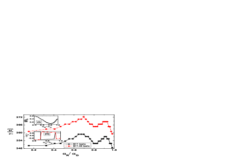
Figure 8: (Color online) The Berry phase (absolute value) on the spin state $|0,0,+1\rangle$ vs $\alpha_{R}/\alpha_{D}$ in GaAs QDs. The first maximum in the Berry phase can be seen due to the fact that the $g$-factor of electrons changes its sign (see inset plot (i)). The parameters are chosen the same as in Fig. 1 but $\ell_{0}=35$ nm and $B=1$T. Inset plot (ii) shows $\langle\sigma_{z}\rangle$ for the states $|0,0,-1\rangle$ (solid line) and for the states $|0,0,+1\rangle$ (dashed-dotted line).

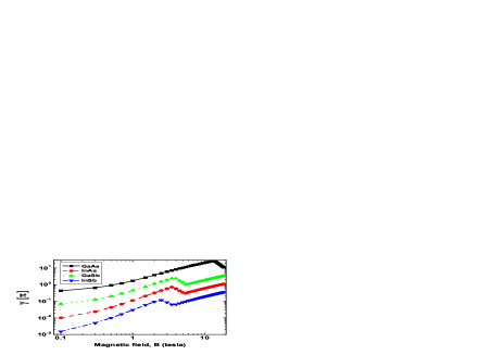
Figure 9: (Color online) The Berry phase (absolute value) on the spin state $|0,0,+1\rangle$ vs longitudinal magnetic field in III-V semiconductor QDs. Here we choose $E_{z}=3\times 10^{5}~{}V/cm$ and $\ell_{0}=20$ nm. Notice that the Berry phase terminates at the crossing point.

We now turn to the calculation of the Berry phase. If the QD is adiabatically carried around a circle of radius $r_{0}$, the wavefunction acquires a geometric phase, Berry (1984); Wilczek and Zee (1984)

$$\gamma_{n}=-Im\int_{S}d\mathbf{S}\mbox{\boldmath${\cdot}$}\sum_{m\neq n}\frac{\langle n|\mbox{\boldmath${\nabla_{E}}$}\hat{H}|m\rangle\mbox{\boldmath${\times}$}\langle m|\mbox{\boldmath${\nabla_{E}}$}\hat{H}|n\rangle}{\left\{\varepsilon_{m}(\mathbf{E})-\varepsilon_{n}(\mathbf{E})\right\}^{2}},$$ (19)

where $S$ is the area enclosed by the circle. We consider $|n\rangle=|0,0,\pm 1\rangle$ and $|m\rangle=|0,1,\pm 1\rangle$ and investigate the Berry phase in QD accumulated during the adiabatic transport of the dot in the plane of 2DEG. Other choices of the parameters such as $|m\rangle=|1,0,\pm 1\rangle$ also induce a non-zero Berry phase on $|n\rangle=|0,0,\pm 1\rangle$ which is comparatively very small. Based on the second order perturbation theory, after lengthy algebraic transformations, Eq. (19) can be written as

$$\gamma_{0,0,\pm 1}=\mp\frac{\pi}{2}\frac{\left(\hbar\omega_{+}\xi_{-}r_{0}\right)^{2}}{\left[\hbar\Omega_{-}\pm\xi_{-}^{2}\left(\frac{\alpha_{R}^{2}}{\varrho_{+}}-\frac{\alpha_{D}^{2}}{\varrho_{-}}\right)\right]^{2}},$$ (20)

where $\varrho_{\pm}=\hbar\Omega_{-}\pm\Delta$. Berry phase (20) can also be expressed in terms of three relevant length scales, SO lengths ($\lambda_{R}$ and $\lambda_{D}$), hybrid orbital length ($\ell=\sqrt{\hbar/m\Omega}$) and orbital radius $(r_{0}=meE_{0}\ell^{4}_{0}/\hbar^{2})$, as:

$$\gamma_{0,0,\pm 1}=\mp\frac{\pi}{2}\frac{\left(\ell\omega_{+}r_{0}\right)^{2}\left(2\hbar-eB\ell\right)^{2}}{\left[\hbar\ell\Omega_{-}\pm\zeta\left(2\hbar-eB\ell\right)^{2}\left(\lambda_{D}^{2}\varrho_{-}-\lambda_{R}^{2}\varrho_{+}\right)\right]^{2}},$$ (21)

where $\zeta=\hbar^{2}/2m^{2}\varrho_{+}\varrho_{-}\lambda_{R}^{2}\lambda_{D}^{2}$. The characteristics of the Berry phase for three relevant length scales (SO lengths, hybrid orbital length and orbital radius) are discussed in Figs. 5 and 6.

III Computational Method

We suppose that a QD is formed in the plane of a two dimensional electron gas of $400\times 400~{}\mathrm{nm^{2}}$ geometry. Then we vary the in-plane oscillating electric fields $E_{x}(t)$ and $E_{y}(t)$ adiabatically in such a way that the QD is transported in a closed loop of circular trajectory (see Fig. 1). To find the Berry phase using an explicit numerical method, we diagonalize the total Hamiltonian $H(t)$ at any fixed time using the finite element method. The geometry contains $24910$ elements. Since the geometry is much larger compared to the actual lateral size of the QD, we impose Dirichlet boundary conditions and find the eigenvalues and eigenfunctions of the total Hamiltonian $H(t)$. In Figs. 5 and 6, the analytically obtained Berry phase from Eq. (21) (solid and dashed-dotted lines) is seen to be in excellent agreement with the numerical values (circles and squares). Figs. 7, 8 and  9 are obtained by solving the Hamiltonian $H(t)$ via the exact diagonalization method. The material constants for GaAs, InAs, GaSb and InSb semiconductors are taken from Ref. Prabhakar et al., 2013.

IV Results and Discussions

In Fig. 1, the realistic electron wavefunctions of the dots at different locations ($\theta=0,\pi/2,\pi,3\pi/2$) are shown. The evolution of spin dynamics in the expectation values of the Pauli spin matrices, due to adiabatic Rashba-Dresselhaus spin-orbit couplings in (8), is shown in Fig. 2. In the presence of both the Rashba and the Dresselhaus spin-orbit couplings, we find the spin-echo due to a superposition of spin waves in the evolution of spin dynamics during the adiabatic transport of the dots in the 2D plane (for details, see appendix B and Fig. 3).

Since we know the exact unitary operator, it is possible to realize the quantum gates (see Fig. 4) during the adiabatic transport of the dots. Bednarek et al. (2012, 2008); Amparan et al. (2013) In Fig. 4, we plot gate fidelity versus rotation angle. Here we express the probability in terms of gate fidelity equal to $|\langle\Psi_{obj}|\chi\left(\theta\right)\rangle|^{2}$, where the objective or ideal vector state $|\Psi_{obj}\rangle$ is the product of the gate operation (Pauli matrix) on the initial state $|\chi\left(\theta=0\right)\rangle$ and $|\chi\left(\theta\right)\rangle$ is to evolve the dynamics of the unitary operator (see Eq. B). Amparan et al. (2013) It can be seen that one can observe the perfect fidelity (i.e. fidelity=1) at $\theta=29\pi$ (solid line), $\theta=8\pi$ (dashed line) and $\theta=23\pi$ (dashed-dotted line). Thus one can find the Pauli-X, Pauli-Y and Pauli-Z gates at $\theta=29\pi,8\pi$ and $23\pi$ respectively. Recently similar kind of results for the realization of Pauli gates from symmetric graphene quantum dots by utilizing the genetic algorithm Chong and Żak (2001) have also been presented in Ref. Amparan et al., 2013.

We now turn to another key result of the paper: the analysis of the Berry phase accumulated during the adiabatic transport of the dots in the 2D plane. In Fig. 5, we plot the characteristics of the Berry phase versus three relevant length scales (SO length (left panel), orbital radius and hybrid orbital length (right panel)). As can be seen (left panel of Fig. 5), the Berry phase for the pure Rashba and pure Dresselhaus cases is well separated at smaller values of the SO lengths due to the presence of different symmetry orientations in the crystal lattice, such as a lack of structural inversion asymmetry along the growth direction for the Rashba case and the bulk inversion asymmetry for the Dresselhaus spin-orbit coupling case [see Eq. 22]. At large values of SO lengths $\lambda_{R}=\lambda>1.8\mu m$, the Berry phases for the pure Rashba and for the pure Dresselhaus spin-orbit coupling cases meet each other because the SO coupling strength is extremely weak and is unable to break the in-plane rotational symmetry. Note that the SO length is characterized by the applied electric field along the z-direction (inset plot of the left panel in Fig. 5 and also see Eqs. (2) and (3)). Prabhakar et al. (2013) In the right panel of Fig. 5 (solid line), we see that the Berry phase decreases with increasing values of hybrid orbital length. This occurs because the hybrid orbital length is inversely proportional to the applied magnetic field that reduce the energy difference between the corresponding spin states. Also, in the right panel of Fig. 5 (dashed dotted line), we see that the Berry phase increases with increasing values of orbital radius because of the enhancement in the total enclosed adiabatic area. Figure 6 investigates the characteristics of the Berry phase in InAs QDs with three relevant lengths: SO length, hybrid orbital length and QDs radii. For the pure Rashba case after the level crossing point at $\lambda_{R}=0.06~{}\mu m$, the analytically obtained values from Eq. (21) capture the Berry phase on the state $|0,0,-1\rangle$.

In Fig. 7(a), the abrupt changes (i.e. the first maximum or minimum) in tunability of the Berry phase at $\alpha_{R}/\alpha_{D}\approx 0.8$ are possible since the Bloch wavefunctions can be pushed near the edge of the barrier materials but are still located in the QD region because the effective $g$-factor of electrons is still negative (see intet plot, Fig. 7(a)(i)). The second maximum or minimum in the Berry phase at $\alpha_{R}/\alpha_{D}\approx 1.15$ can be seen due to the sign change in the $g$-factor of the p-state (see inset plot Fig. 7(a)(ii)). In Fig. 7(b), we study the Berry phase in InAs QDs.

Let us consider the quantitative difference between the Berry phases accumulated on the electron spin states $|0,0,\pm 1\rangle$. For simplicity, we only consider the second powers of the Rashba-Dresselhaus spin-orbit couplings:

$$\sqrt{\frac{\gamma_{0,0,+1}}{\gamma_{0,0,-1}}}=1-\frac{2m}{\hbar^{3}\Omega}\left[\alpha_{R}^{2}\left(1-\frac{\Delta}{\hbar\Omega_{-}}\right)-\alpha_{D}^{2}\left(1+\frac{\Delta}{\hbar\Omega_{-}}\right)\right].$$ (22)

In InAs and InSb QDs, $\alpha_{R}>\alpha_{D}$. It means, $\gamma_{0,0,-1}>\gamma_{0,0,+1}$ and viceversa for GaAs and GaSb QDs.

In Fig. 8, we find that the large enhancement in the Berry phase occurs with a very small increment in the magnetic fields. This indicates that the Berry phase is highly sensitive to magnetic fields in QDs. The first maximum (approx. $\alpha_{R}/\alpha_{D}=0.67$) in the Berry phase results from the sign change in the $g$-factor of electrons in QDs (see the inset plot of Fig.8). This means that the Bloch wavefunctions start penetrating into the barrier materials. Experimentally, the penetration of the Bloch wavefunctions in the AlGaAs/GaAs heterojunction can be engineered with the application of gate controlled electric fields along the z direction where the bulk $g$-factor of electrons for GaAs materials is negative, and for AlGaAs it is positive. Jiang and Yablonovitch (2001) The second maximum (at $\alpha_{R}/\alpha_{D}=0.9$) can be seen due to the fact that the wavefunctions of electrons are pushed back into the GaAs material. The minimum point (at $\alpha_{R}/\alpha_{D}=0.9$) in the Berry phase and in the $g$-factor indicates that the Bloch wavefunctions are getting pushed towards the QD region due to the interplay between the Rashba and the Dresselhaus spin-orbit couplings. Fig. 9 investigates the Berry phase versus magnetic fields in III-V semiconductor QDs.

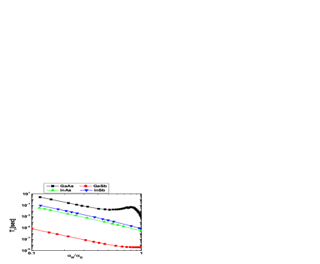
Figure 10: (Color online) Spin relaxation time, $T_{1}$ vs $\alpha_{R}/\alpha_{D}$ in a moving QD at location $\theta=0$ (see Fig. 1). We choose $B=1$ T, $\ell_{0}=20$ nm and $E_{0}=5\times 10^{3}$ V/cm. The material constants are chosen from Ref. de Sousa and Das Sarma, 2003.

Spin relaxation: Now we estimate the spin relaxation time caused by the emission of one phonon at absolute zero temperature between two lowest energy states in III-V semiconductor QDs. Since we deal with small energy transfer between electron in QDs and phonon, we only consider a piezo-phonon.Khaetskii and Nazarov (2001) Hence coupling between an electron and a piezo-phonon with mode $\mathbf{q}\alpha$ ($\mathbf{q}$ is the phonon wave vector and the branch index $\alpha=l,t_{1},t_{2}$ for one longitudinal and two transverse modes) is given by: Khaetskii and Nazarov (2001); de Sousa and Das Sarma (2003); Prabhakar et al. (2013)

$$u^{\mathbf{q}\alpha}_{\mathrm{ph}}\left(\mathbf{r},t\right)=\sqrt{\frac{\hbar}{2\rho V\omega_{\mathbf{q}\alpha}}}e^{i\left(\mathbf{q\cdot r}-\omega_{q\alpha}t\right)}eA_{\mathbf{q}\alpha}b^{{\dagger}}_{\mathbf{q}\alpha}+\mathrm{H.c.},$$ (23)

where $\rho$ is the crystal mass density, $V$ is the volume of the QD and $A_{\mathbf{q}\alpha}=\hat{q}_{i}\hat{q}_{k}e\beta_{ijk}e^{j}_{\mathbf{q}\alpha}$ is the amplitude of the electric field created by phonon strain. Here $\hat{\mathbf{q}}=\mathbf{q}/q$ and $e\beta_{ijk}=eh_{14}$ for $i\neq k,i\neq j,j\neq k$. Based on the Fermi Golden Rule, the phonon induced spin transition rate in the QDs is given by de Sousa and Das Sarma (2003); Khaetskii and Nazarov (2001)

$$\frac{1}{T_{1}}=\frac{2\pi}{\hbar}\int\frac{d^{3}\mathbf{q}}{\left(2\pi\right)^{3}}\sum_{\alpha=l,t}\arrowvert M\left(\mathbf{q}\alpha\right)\arrowvert^{2}\delta\left(\hbar s_{\alpha}\mathbf{q}-\varepsilon_{f}+\varepsilon_{i}\right),$$ (24)

The matrix element $M\left(\mathbf{q}\alpha\right)=\langle\psi_{i}|u^{\mathbf{q}\alpha}_{ph}\left(\mathbf{r},t\right)|\psi_{f}\rangle$ has been calculated numerically. Prabhakar et al. (2013); com Here $|\psi_{i}\rangle$ and $|\psi_{f}\rangle$ correspond to the initial and finial states of the Hamiltonian $H$.

In Fig. 10, we plotted the spin relaxation time versus the interplay between the Rashba and Dresselhaus spin-orbit coupling strengths. Different behavior of spin-relaxation in GaAs is observed due to the fact that the $g$-factor of electron spin in GaAs QDs changes its sign (see the inset plot of Fig. 8). Evidently large spin relaxation time, $T_{1}$ and thus decoherence time, $T_{2}\approx 2T_{1}$ can be seen in GaAs QDs.

Long decoherence time combined with short gate operation time is one of the requirements for quantum computing and quantum information processing. Loss and DiVincenzo (1998); Awschalom et al. (2002); Bandyopadhyay (2000) However, at (or near by) the level crossing point in the Berry phase, a spin-hot spot can be observed that greatly reduces the decoherence time. Bulaev and Loss (2005a, b); de Sousa and Das Sarma (2003); Prabhakar et al. (2013) Thus one should avoid such level crossing points in the Berry phase during the design of QD spin-based transistors for possible implementation in solid-state quantum computing and quantum information processing. When a qubit is operated on by a classical bit, then its decay time is given by a spin-relaxation time which is also supposed to be longer than the minimum time required to execute one quantum gate operation. Amasha et al. (2008); Pribiag et al. (2013) It seems that the spin-relaxation time in GaAs QD is much larger than in other materials (InAs, InSb and GaSb) due to the presence of weak spin-orbit coupling. Prabhakar et al. (2013); Bulaev and Loss (2005a, b) However, other factors such as mobility of the charge carriers and defects might greatly affect the performance of gate operation time, and hence decoherence time. Thus, additional experimental studies may be required to show that GaAs is indeed a better candidate for quantum gate operations. Enhancement in the Berry phase of GaAs QDs and extension of the level crossing point, such as to larger QDs radii as well as to larger magnetic fields, might provide some additional benefits to control electron spins for larger lateral size QDs when choosing GaAs material rather than InAs, InSb, or GaSb.

Finally, we mention a possible experimental realization of the measurement of the Berry phase in QDs. Several parameters such as $E_{x}(t)$, $E_{y}(t)$ and $\theta$ in the distortion potential can relate to the other control parameters, $\alpha_{R}$, $\alpha_{D}$, $\omega_{0}$, and $\Delta/\hbar$ of the dots, so that one can experimentally realize the adiabatic movement of the QDs in the 2D plane. Following Refs. Berger et al., 2012; Pechal et al., 2012; Yang and Hwang, 2006; Bason et al., 2012, the adiabatic movement of the dots can be performed by choosing the frequency $\omega$ of the microwave pulse smaller than $\varepsilon^{0}_{0,0,\pm 1}/\hbar$ and $\omega_{0}$. Also, we chose $E_{0}\ll E_{z}$ to study the interplay between the Rashba and the Dresselhaus spin-orbit couplings on the Berry phase.

V Conclusion

We have calculated the evolution of the spin dynamics and the superposition due to the Rashba-Dresselhaus spin-orbit couplings that can be seen during the adiabatic transport of QDs in the 2D plane. We have shown that the Berry phase in the lowest Landau levels of the QD can be generated from higher quantum states that only differ by one quantum number of the corresponding spin states. The Berry phase is highly sensitive to the magnetic fields, QD radii, and the Rashba-Dresselhaus spin-orbit coupling coefficients. We have shown that the sign change in the $g$-factor in the Berry phase can be manipulated with the interplay between the Rashba and the Dresselhaus spin-orbit couplings. We have provided a detailed analysis of the characteristics of the Berry phase with three relevant length scales (SO length, hybrid orbital length and orbital radius). The sets of data, which can be encoded at the degenerate sub-levels (i.e. at $g=0$) but well separated in their phase, are topologically protected and can help to build a topological solid-state quantum computer.

VI Acknowledgements:

This work was supported by NSERC and CRC programs, Canada. The authors acknowledge Prof. Akira Inomata from the State University of New York at Albany for his many helpful discussions. The authors also acknowledge the Shared Hierarchical Academic Research Computing Network (SHARCNET) community and Dr. P.J. Douglas Roberts for his assistance and technical support.

Appendix A Induced magnetic field due to oscillating electric field

Induced displacement current density due to oscillating electric field is given by

$$\mathbf{J_{in}}=\epsilon_{0}\epsilon_{r}\frac{\partial\mathbf{E}(\mathbf{r})}{\partial t}=\frac{\epsilon_{0}\epsilon_{r}\omega E_{0}}{r_{0}}\left(y_{0},-x_{0}\right),$$ (25)

where $x_{0}=-r_{0}\cos\omega t$, $y_{0}=-r_{0}\sin\omega t$, $\epsilon_{r}$ is the relative permittivity and $\epsilon_{0}$ is the permittivity of the free space. The induced current due to $\mathbf{J_{in}}$ is approximated as

$$I_{in}=\pi r_{0}^{2}|\mathbf{J_{in}}|=\pi r_{0}^{2}\epsilon_{0}\epsilon_{r}\omega E_{0}.$$ (26)

We apply Ampere’s law to estimate the induced $B$ field at the center of the orbit:

$$B_{z}=\frac{\mu_{0}\mu_{r}I_{in}}{2r_{0}}=\frac{\pi\epsilon_{r}\mu_{r}r_{0}\omega E_{0}}{2c^{2}},$$ (27)

where $\mu_{r}$ is the relative permeability and $c=1/\sqrt{\epsilon_{0}\mu_{0}}$ is the velocity of light with $\mu_{0}$ being the permeability of the free space.

Appendix B Exact unitary operator of spin Hamiltonian

To investigate the evolution of spin dynamics due to adiabatic parameters in the Hamiltonian ((8), we write the adiabatic Rashba-Dresselhaus spin-orbit couplings as

$$h_{ad}=\frac{1}{\hbar}\left(\alpha_{R}z_{-}-i\alpha_{D}z_{+}\right)m\omega_{+}s_{+}+H.c.,$$ (28)

where $s_{\pm}=s_{x}\pm is_{y}$. We construct a normalized orthogonal set of eigenspinors of Hamiltonian (28) as:

$$\mathbf{\chi_{+}}\left(t\right)=\frac{1}{\sqrt{2}}\left(\begin{array}[]{c}1\\ \frac{\left[\alpha_{1}^{2}+\beta_{1}^{2}+2\alpha_{1}\beta_{1}\sin 2\omega t\right]^{1/2}}{i\beta_{1}\exp\left(i\omega t\right)-\alpha_{1}\exp\left(-i\omega t\right)}\\ \end{array}\right),$$ (31)

$$\mathbf{\chi_{-}}\left(t\right)=\frac{1}{\sqrt{2}}\left(\begin{array}[]{c}\frac{i\beta_{1}\exp\left(i\omega t\right)-\alpha_{1}\exp\left(-i\omega t\right)}{\left[\alpha_{1}^{2}+\beta_{1}^{2}+2\alpha_{1}\beta_{1}\sin 2\omega t\right]^{1/2}}\\ -1\\ \end{array}\right),$$ (34)

where $\alpha_{1}=\alpha_{R}r_{0}m\omega_{+}/\hbar$, $\beta_{1}=\alpha_{D}r_{0}m\omega_{+}/\hbar$. Following Ref. (Prabhakar et al., 2010), by utilizing the disentangling operator technique, the exact evolution operator of (28) for a spin-1/2 particle can be written as:

$$U(t) = \tau\exp\left\{\frac{-i}{\hbar}\int h_{ad}~{}d\tau\right\},$$ (35)

$$= \left(\begin{array}[]{cc}\exp\left\{{\frac{b}{2}}\right\}+ac\exp\left\{{-\frac{b}{2}}\right\}&~{}~{}~{}a\exp\left\{-{\frac{b}{2}}\right\}\\ c\exp\left\{-{\frac{b}{2}}\right\}&~{}~{}~{}\exp\left\{-{\frac{b}{2}}\right\}\end{array}\right),~{}~{}~{}~{}~{}$$ (38)

where $\tau$ is a time ordering parameter. The components of the evolution operator follow the relation: $U_{22}=\mathrm{conj}(U_{11})$ and $U_{12}=-\mathrm{conj}(U_{21})$. The $\theta$ dependent functions $a(\theta)$, $b(\theta)$, and $c(\theta)$ are written in terms of adiabatic control parameters $x_{0}$ and $y_{0}$ as:

$$\frac{da}{d\theta}=\frac{i}{\hbar^{2}}m\varpi_{+}\{\left(-\alpha_{-}x_{0}+i\alpha_{+}y_{0}\right)$$

$$+a^{2}\left(\alpha_{+}x_{0}+i\alpha_{-}y_{0}\right)\},$$ (39)

$$\frac{db}{d\theta}=\frac{2i}{\hbar^{2}}m\varpi_{+}\left(\alpha_{+}x_{0}+i\alpha_{-}y_{0}\right)a,$$ (40)

$$\frac{dc}{d\theta}=-\frac{i}{\hbar^{2}}m\varpi_{+}\left(\alpha_{+}x_{0}+i\alpha_{-}y_{0}\right)e^{b},$$ (41)

where $\alpha_{\pm}=\alpha_{R}\pm i\alpha_{D}$ and $\varpi_{+}=1+\omega_{c}/(2\omega)$. At $\theta=0$, we use the initial condition $\chi\left(0\right)=\left(1~{}\sqrt{\alpha_{1}^{2}+\beta_{1}^{2}}/\left(i\beta_{1}-\alpha_{1}\right)\right)^{\top}/\sqrt{2}$, where $\top$ denotes transpose and write $\chi\left(t\right)=U(t,0)\chi\left(0\right)$ as

$$\chi\left(t\right)=\frac{1}{\sqrt{2}}\left(\begin{array}[]{c}e^{b/2}+ace^{-b/2}+\left(\frac{\sqrt{\alpha_{1}^{2}+\beta_{1}^{2}}}{i\beta_{1}-\alpha_{1}}\right)ae^{-b/2}\\ ce^{-b/2}+\left(\frac{\sqrt{\alpha_{1}^{2}+\beta_{1}^{2}}}{i\beta_{1}-\alpha_{1}}\right)e^{-b/2}\end{array}\right).$$

By using Eq. (B), we found expectation values of Pauli spin matrices and plotted them in Fig. 2. Components of the evolution operator of (38) are shown in Fig. 3. The exact probabilities of a transition to spin up (solid line) and spin down (dashed-dotted line) are shown in Fig. 11 during the adiabatic movement of the QDs in the 2D plane. It can be seen that the sum of spin up and spin down probabilities are always unity (dotted line of Fig. 11) which indicates that the evolution operator (38) of the quasi-Hamiltonian (28) is exact and the symmetry of the unitary operator during the adiabatic movement of dots is preserved.

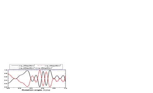
Figure 11: (Color online) The exact probability of a transition to spin up (solid line) and spin down (dashed-dotted line) vs rotation angle. The parameters are chosen the same as in Fig. 2.

In order to verify that the evolution operator (38) is indeed exact and unitary to (35), we expand (35) for the pure Rashba case by following Dyson series method as:

$$U(t) = 1+i\tilde{r}_{0}\left\{\sigma_{x}\sin\theta+\sigma_{y}\left(1-\cos\theta\right)\right\}-\tilde{r}^{2}_{0}\left\{-i\sigma_{z}\left(\theta-\sin\theta\right)+\left(1-\cos\theta\right)\right\}$$ (42)

$$-i\tilde{r}^{3}_{0}\left\{\sigma_{x}\left(2\sin\theta-\theta\cos\theta-\theta\right)+\sigma_{y}\left(-2\cos\theta-\theta\sin\theta+2\right)\right\}$$

$$+\tilde{r}^{4}_{0}\left\{i\sigma_{z}\left(-2\theta+3\sin\theta-\theta\cos\theta\right)+\left(-\frac{1}{2}\theta^{2}-3\cos\theta-\theta\sin\theta+3\right)\right\}+O(\tilde{r}^{5}_{0}),$$

where $\tilde{r}_{0}=\alpha_{R}m\varpi_{+}r_{0}/\hbar^{2}$. Next we write evolution operator (38) as

$$U(t)=U_{0}I+U_{x}\sigma_{x}+U_{y}\sigma_{y}+U_{z}\sigma_{z},$$ (43)

where

$$U_{0}=\frac{1}{2}\left\{\exp\left(\frac{b}{2}\right)+ac\exp\left(\frac{b}{2}\right)+\exp\left(-\frac{b}{2}\right)\right\},~{}~{}~{}~{}~{}~{}~{}~{}$$ (44)

$$U_{x}=\frac{1}{2}\left\{a\exp\left(-\frac{b}{2}\right)+c\exp\left(-\frac{b}{2}\right)\right\},~{}~{}~{}~{}~{}~{}~{}~{}~{}$$ (45)

$$U_{y}=\frac{i}{2}\left\{a\exp\left(-\frac{b}{2}\right)-c\exp\left(-\frac{b}{2}\right)\right\},~{}~{}~{}~{}~{}~{}~{}~{}~{}$$ (46)

$$U_{z}=\frac{1}{2}\left\{\exp\left(\frac{b}{2}\right)+ac\exp\left(-\frac{b}{2}\right)-\exp\left(-\frac{b}{2}\right)\right\}.~{}~{}~{}~{}~{}~{}~{}~{}$$ (47)

The functions $a(\theta)$, $b(\theta)$, $c(\theta)$ are obtained by solving three coupled Riccatti Eqs. (39), (40), (41) for the pure Rashba case as

$$a(\theta)=\frac{2\tilde{r}_{0}\left\{\exp(-in_{1}\theta)-\exp\left(-i\theta\right)\right\}}{n_{2}-n_{1}\exp\left\{-i\left(n_{1}-1\right)\theta\right\}},$$ (48)

$$\exp(b(\theta)/2)=\frac{2\left(n_{1}-1\right)\exp(-in_{1}\theta/2)}{n_{1}\exp\left\{-i\left(n_{1}-1\right)\theta\right\}-n_{2}},$$ (49)

$$c(\theta)=\frac{2\tilde{r}_{0}\left\{1-\exp\left[-i\left(n_{1}-1\right)\theta\right]\right\}}{n_{1}\exp\left\{-i\left(n_{1}-1\right)\theta\right\}-n_{2}},$$ (50)

where

$$n_{1,2}=1\pm\sqrt{1+4\tilde{r}^{2}_{0}}.$$ (51)

By substituting Eqs. (48), (49) and (50) in Eqs. (44), (45), (46) and (47), we find

$$U_{0}=1+2\frac{\tilde{r}^{2}_{0}}{2!}\left(\cos\theta-1\right)+24\frac{\tilde{r}^{4}_{0}}{4!}\left(3-\frac{1}{2}\theta^{2}-\theta\sin\theta-3\cos\theta\right)+O\left(\tilde{r}^{6}_{0}\right),$$ (52)

$$U_{x}=i\tilde{r}_{0}\sin\theta+6i\frac{\tilde{r}^{3}_{0}}{3!}\left(-2\sin\theta+\theta\cos\theta+\theta\right)+O\left(\tilde{r}^{5}_{0}\right),$$ (53)

$$U_{y}=i\tilde{r}_{0}\left(1-\cos\theta\right)+6i\frac{\tilde{r}^{3}_{0}}{3!}\left(-2+2\cos\theta+\theta\sin\theta\right)+O\left(\tilde{r}^{5}_{0}\right),$$ (54)

$$U_{z}=2i\frac{\tilde{r}^{2}_{0}}{2!}\left(\theta-\sin\theta\right)+24i\frac{\tilde{r}^{4}_{0}}{4!}\left(-2\theta-\theta\cos\theta+3\sin\theta\right)+O\left(\tilde{r}^{5}_{0}\right).$$ (55)

One can easily identify that the coefficients $U_{0}$, $U_{x}$, $U_{y}$ and $U_{z}$ of Eq. (43) are exactly the same as in Eq. (42). Thus the evolution operator (38) obtained by the Feynman disentangling operator scheme is exact for any order of the orbital radius.

References

- Amasha et al. (2008) S. Amasha, K. MacLean, I. P. Radu, D. M. Zumbühl, M. A. Kastner, M. P. Hanson, and A. C. Gossard, Phys. Rev. Lett. 100, 046803 (2008).
- Takahashi et al. (2010) S. Takahashi, R. S. Deacon, K. Yoshida, A. Oiwa, K. Shibata, K. Hirakawa, Y. Tokura, and S. Tarucha, Phys. Rev. Lett. 104, 246801 (2010).
- Prabhakar et al. (2013) S. Prabhakar, R. Melnik, and L. L. Bonilla, Phys. Rev. B 87, 235202 (2013).
- Awschalom et al. (2002) D. D. Awschalom, D. Loss, and N. Samarth, Semiconductor Spintronics and Quantum Computation (Springer, Berlin, 2002).
- Loss and DiVincenzo (1998) D. Loss and D. P. DiVincenzo, Phys. Rev. A 57, 120 (1998).
- Prabhakar and Raynolds (2009) S. Prabhakar and J. E. Raynolds, Phys. Rev. B 79, 195307 (2009).
- Prabhakar et al. (2011) S. Prabhakar, J. E. Raynolds, and R. Melnik, Phys. Rev. B 84, 155208 (2011).
- de Sousa and Das Sarma (2003) R. de Sousa and S. Das Sarma, Phys. Rev. B 68, 155330 (2003).
- Prabhakar et al. (2012) S. Prabhakar, R. V. N. Melnik, and L. L. Bonilla, Applied Physics Letters 100, 023108 (2012).
- Bandyopadhyay (2000) S. Bandyopadhyay, Phys. Rev. B 61, 13813 (2000).
- Flatté (2011) M. E. Flatté, Physics 4, 73 (2011).
- Giuliano et al. (2003) D. Giuliano, P. Sodano, and A. Tagliacozzo, Phys. Rev. B 67, 155317 (2003).
- Aleiner and Fal’ko (2001) I. L. Aleiner and V. I. Fal’ko, Phys. Rev. Lett. 87, 256801 (2001).
- Wang and Zhu (2008) H. Wang and K.-D. Zhu, EPL 82, 60006 (2008).
- Yang and Hwang (2006) S.-R. E. Yang and N. Y. Hwang, Phys. Rev. B 73, 125330 (2006).
- Eric Yang (2006) S.-R. Eric Yang, Phys. Rev. B 74, 075315 (2006).
- Yang (2007) S.-R. E. Yang, Phys. Rev. B 75, 245328 (2007).
- Berry (1984) M. V. Berry, Proceedings of the Royal Society of London. Series A, Mathematical and Physical Sciences 392, 45 (1984).
- Wilczek and Zee (1984) F. Wilczek and A. Zee, Phys. Rev. Lett. 52, 2111 (1984).
- Prabhakar et al. (2010) S. Prabhakar, J. Raynolds, A. Inomata, and R. Melnik, Phys. Rev. B 82, 195306 (2010).
- Pechal et al. (2012) M. Pechal, S. Berger, A. A. Abdumalikov, J. M. Fink, J. A. Mlynek, L. Steffen, A. Wallraff, and S. Filipp, Phys. Rev. Lett. 108, 170401 (2012).
- Berger et al. (2012) S. Berger, M. Pechal, S. Pugnetti, A. A. Abdumalikov, L. Steffen, A. Fedorov, A. Wallraff, and S. Filipp, Phys. Rev. B 85, 220502 (2012).
- Leek et al. (2007) P. J. Leek, J. M. Fink, A. Blais, R. Bianchetti, M. Goppl, J. M. Gambetta, D. I. Schuster, L. Frunzio, R. J. Schoelkopf, and A. Wallraff, Science 318, 1889 (2007).
- Das Sarma et al. (2005) S. Das Sarma, M. Freedman, and C. Nayak, Phys. Rev. Lett. 94, 166802 (2005).
- Hu and Das Sarma (2000) X. Hu and S. Das Sarma, Phys. Rev. A 61, 062301 (2000).
- Loss et al. (1990) D. Loss, P. Goldbart, and A. V. Balatsky, Phys. Rev. Lett. 65, 1655 (1990).
- Tserkovnyak and Loss (2011) Y. Tserkovnyak and D. Loss, Phys. Rev. A 84, 032333 (2011).
- San-Jose et al. (2006) P. San-Jose, G. Zarand, A. Shnirman, and G. Schön, Phys. Rev. Lett. 97, 076803 (2006).
- San-Jose et al. (2008) P. San-Jose, B. Scharfenberger, G. Schön, A. Shnirman, and G. Zarand, Phys. Rev. B 77, 045305 (2008).
- San-Jose et al. (2007) P. San-Jose, G. Sch n, A. Shnirman, and G. Zarand, Physica E 40, 76 (2007).
- Jones et al. (2000) J. A. Jones, V. Vedral, A. Ekert, and G. Castagnoli, Nature 403, 869 (2000).
- Falci et al. (2000) G. Falci, R. Fazio, G. M. Palma, J. Siewert, and V. Vedral, Nature 407, 355 (2000).
- Xiao et al. (2010) D. Xiao, M.-C. Chang, and Q. Niu, Rev. Mod. Phys. 82, 1959 (2010).
- Nayak et al. (2008) C. Nayak, S. H. Simon, A. Stern, M. Freedman, and S. Das Sarma, Rev. Mod. Phys. 80, 1083 (2008).
- Bychkov and Rashba (1984) Y. A. Bychkov and E. I. Rashba, J. Phys. C 17, 6039 (1984).
- Dresselhaus (1955) G. Dresselhaus, Phys. Rev. 100, 580 (1955).
- Bason et al. (2012) M. G. Bason, M. Viteau, N. Malossi, P. Huillery, E. Arimondo, D. Ciampini, R. Fazio, V. Giovannetti, R. Mannella, and O. Morsch, Nat. Phys. 8, 147 (2012).
- Ban et al. (2012) Y. Ban, X. Chen, E. Y. Sherman, and J. G. Muga, Phys. Rev. Lett. 109, 206602 (2012).
- Prabhakar et al. (2014) S. Prabhakar, R. Melnik, and A. Inomata, Applied Physics Letters 104, 142411 (2014).
- Bednarek et al. (2012) S. Bednarek, J. P. owski, and A. Skubis, Applied Physics Letters 100, 203103 (2012).
- Bednarek et al. (2008) S. Bednarek, B. Szafran, R. J. Dudek, and K. Lis, Phys. Rev. Lett. 100, 126805 (2008).
- Bednarek and Szafran (2008) S. Bednarek and B. Szafran, Phys. Rev. Lett. 101, 216805 (2008).
- Wu et al. (2011) Y. Wu, I. M. Piper, M. Ediger, P. Brereton, E. R. Schmidgall, P. R. Eastham, M. Hugues, M. Hopkinson, and R. T. Phillips, Phys. Rev. Lett. 106, 067401 (2011).
- Golovach et al. (2006) V. N. Golovach, M. Borhani, and D. Loss, Phys. Rev. B 74, 165319 (2006).
- Saniz et al. (2003) R. Saniz, B. Barbiellini, A. B. Denison, and A. Bansil, Phys. Rev. B 68, 165326 (2003).
- Amparan et al. (2013) G. Amparan, F. Rojas, and A. Perez-Garrido, Nanoscale Research Letters 8, 242 (2013).
- Chong and Żak (2001) E. K. P. Chong and S. H. Żak, An Introduction to Optimization (John Wiley and Sons, Inc., 2001).
- Jiang and Yablonovitch (2001) H. W. Jiang and E. Yablonovitch, Phys. Rev. B 64, 041307 (2001).
- Khaetskii and Nazarov (2001) A. V. Khaetskii and Y. V. Nazarov, Phys. Rev. B 64, 125316 (2001).
- (50) Comsol Multiphysics version 3.5a (www.comsol.com).
- Bulaev and Loss (2005a) D. V. Bulaev and D. Loss, Phys. Rev. Lett. 95, 076805 (2005a).
- Bulaev and Loss (2005b) D. V. Bulaev and D. Loss, Phys. Rev. B 71, 205324 (2005b).
- Pribiag et al. (2013) V. S. Pribiag, S. Nadj-Perge, S. M. Frolov, J. W. G. van den Berg, I. van Weperen, S. R. Plissard, E. P. A. M. Bakkers, and L. P. Kouwenhoven, Nature nanotechnology 8, 170 (2013).