High-dimensionality effects in the Markowitz problem and other quadratic programs with linear constraints: Risk underestimation

Abstract

We first study the properties of solutions of quadratic programs with linear equality constraints whose parameters are estimated from data in the high-dimensional setting where $p$, the number of variables in the problem, is of the same order of magnitude as $n$, the number of observations used to estimate the parameters. The Markowitz problem in Finance is a subcase of our study. Assuming normality and independence of the observations we relate the efficient frontier computed empirically to the “true” efficient frontier. Our computations show that there is a separation of the errors induced by estimating the mean of the observations and estimating the covariance matrix. In particular, the price paid for estimating the covariance matrix is an underestimation of the variance by a factor roughly equal to $1-p/n$. Therefore the risk of the optimal population solution is underestimated when we estimate it by solving a similar quadratic program with estimated parameters.

We also characterize the statistical behavior of linear functionals of the empirical optimal vector and show that they are biased estimators of the corresponding population quantities.

We investigate the robustness of our Gaussian results by extending the study to certain elliptical models and models where our $n$ observations are correlated (in “time”). We show a lack of robustness of the Gaussian results, but are still able to get results concerning first order properties of the quantities of interest, even in the case of relatively heavy-tailed data (we require two moments). Risk underestimation is still present in the elliptical case and more pronounced than in the Gaussian case.

We discuss properties of the nonparametric and parametric bootstrap in this context. We show several results, including the interesting fact that standard applications of the bootstrap generally yield inconsistent estimates of bias.

We propose some strategies to correct these problems and practically validate them in some simulations. Throughout this paper, we will assume that $p$, $n$ and $n-p$ tend to infinity, and $p<n$.

Finally, we extend our study to the case of problems with more general linear constraints, including, in particular, inequality constraints.

T1Supported by the France–Berkeley Fund, a Sloan research Fellowship and NSF Grants DMS-06-05169 and DMS-08-47647 (CAREER).

1 Introduction

Many statistical estimation problems are now formulated, implicitly or explicitly, as solutions of certain optimization problems. Naturally, the parameters of these problems tend to be estimated from data and it is therefore important that we understand the relationship between the solutions of two types of optimization problems: those which use the population parameters and those which use the estimated parameters. This question is particularly relevant in high-dimensional inference where one suspects that the differences between the two solutions might be considerable. The aim of this paper is to contribute to this understanding by focusing on quadratic programs with linear constraints. An important example of such a program where our questions are very natural is the celebrated Markowitz optimization problem in Finance which will serve as a supporting example throughout the paper.

The Markowitz problem (Markowitz, 1952) is a classic portfolio optimization problem in Finance, where investors choose to invest according to the following framework: one picks assets in such a way that the portfolio guarantees a certain level of expected returns but minimizes the “risk” associated with them. In the standard framework, this risk is measured the variance of the portfolio.

Markowitz’s paper was highly influential and much work has followed. It is now part of the standard textbook literature on these issues [Ruppert (2006), Campbell, Lo and MacKinlay (1996)]. Let us recall the setup of the Markowitz problem.

• We have the opportunity to invest in $p$ assets, $A_{1},\ldots,A_{p}$.

• In the ideal situation, the mean returns are known and represented by a $p$-dimensional vector, $\mu$.

• Also, the covariance between the returns is known; we denote it by $\Sigma$.

• We want to create a portfolio, with guaranteed mean return $\mu_{P}$, and minimize its risk, as measured by variance.

• The question is how should items be weighted in portfolio? What are weights $w$?

We note that $\Sigma$ is positive semi-definite and hence is in particular symmetric. In the ideal (or population) solution, the covariance and the mean are known. The mathematical formulation is then the following simple quadratic program. We wish to find the weights $w$ that solve the following problem:

$$\cases{\min\frac{1}{2}w^{\prime}\Sigma w,\cr w^{\prime}\mu=\mu_{P},\cr\displaystyle w^{\prime}\mathbf{e}=1.}$$

Here $\mathbf{e}$ is a $p$-dimensional vector with 1 in every entry. If $\Sigma$ is invertible, the solution is known explicitly (see Section 2). If we call $w_{\mathrm{optimal}}$ the solution of this problem, the curve $w_{\mathrm{optimal}}^{\prime}\Sigma w_{\mathrm{optimal}}$, seen as a function of $\mu_{P}$, is called the efficient frontier.

Of course, in practice, we do not know $\mu$ and $\Sigma$ and we need to estimate them. An interesting question is therefore to know what happens in the Markowitz problem when we replace population quantities by corresponding estimators.

Naturally, we can ask a similar question for general quadratic programs with linear constraints [see below or Boyd and Vandenberghe (2004) for a definition], the Markowitz problem being a particular instance of such a problem. This paper provides an answer to these questions under certain distributional assumptions on the data. Hence our paper is really about the impact of estimation error on certain high-dimensional $M$-estimation problems.

It has been observed by many that there are problems in practice when replacing population quantities by standard estimators [see Lai and Xing (2008), Section 3.5], and alternatives have been proposed. A famous one is the Black–Litterman model [Black and Litterman (1990), Meucci (2005) and, e.g., Meucci (2008)]. Adjustments to the standard estimators have also been proposed: Ledoit and Wolf (2004), partly motivated by portfolio optimization problems, proposed to “shrink” the sample covariance matrix toward another positive definite matrix (often the identity matrix properly scaled), while Michaud (1998) proposed to use the bootstrap and to average bootstrap weights to find better-behaved weights for the portfolio. As noted in Lai and Xing (2008), there is a dearth of theoretical studies regarding, in particular, the behavior of bootstrap estimators.

An aspect of the problem that is of particular interest to us is the study of large-dimensional portfolios (or quadratic programs with linear constraints). To make matters clear, we focus on a portfolio with $p=100$ assets. If we use a year of daily data to estimate $\Sigma$, the covariance between the daily returns of the assets, we have $n\simeq 250$ observations at our disposal. In modern statistical parlance, we are therefore in a “large $n$, large $p$” setting, and we know from random matrix theory that $\hat{\Sigma}$ the sample covariance matrix is a poor estimator of $\Sigma$, especially when it comes to spectral properties of $\Sigma$. There is now a developing statistical literature on properties of sample covariance matrices when $n$ and $p$ are both large, and it is now understood that, though $\hat{\Sigma}$ is unbiased for $\Sigma$, the eigenvalues and eigenvectors of $\hat{\Sigma}$ behave very differently from those of $\Sigma$. We refer the interested reader to Johnstone (2001), El Karoui (2007, 2008, 2009a), Bickel and Levina (2008a), Rothman et al. (2008) for a partial introduction to these problems. We wish with this study to make clear that the “large $n$, large $p$” character of the problem has an important impact of the empirical solution of the problem. By contrast, standard but thorough discussions of these problems (Meucci, 2005) give only a cursory treatment of dimensionality issues (e.g., one page out of a whole book).

Another interesting aspect of this problem is that the high-dimensional setting does not allow, by contrast to the classical “small $p$, large $n$” setting, a perturbative approach to go through. In the “small $p$, large $n$” setting, the paper Jobson and Korkie (1980) is concerned, in the Gaussian case, with issues similar to the ones we will be investigating.

The “large $n$, large $p$” setting is the one with which random matrix theory is concerned—and the high-dimensional Markowitz problem has therefore been of interest to random matrix theorists for some time now. We note in particular the paper Laloux et al. (2000), where a random matrix-inspired (shrinkage) approach to improved estimation of the sample covariance matrix is proposed in the context of the Markowitz problem.

Let us now remind the reader of some basic facts of random matrix theory that suggest that serious problems may arise if one solves naively the high-dimensional Markowitz problem or other quadratic programs with linear equality constraints. A key result in random matrix theory is the Marčenko–Pastur equation (Marčenko and Pastur, 1967) which characterizes the limiting distribution of the eigenvalues of the sample covariance matrix and relates it to the spectral distribution of the population covariance matrix. We give only in this introduction its simplest form and refer the reader to Marčenko and Pastur (1967), Wachter (1978), Silverstein (1995), Bai (1999) and, for example, El Karoui (2009a) for a more thorough introduction and very recent developments, as well as potential geometric and statistical limitations of the models usually considered in random matrix theory.

In the simplest setting, we consider data $\{X_{i}\}_{i=1}^{n}$, which are $p$-dimensional. In a financial context, these vectors would be vectors of (log)-returns of assets, the portfolio consisting of $p$ assets. To simplify the exposition, let us assume that the $X_{i}$’s are i.i.d. with distribution ${\cal N}(0,\mathrm{Id}_{p})$. We call $X$ the $n\times p$ matrix whose $i$th row is the vector $X_{i}$. Let us consider the sample covariance matrix

$$\hat{\Sigma}=\frac{1}{n-1}(X-\bar{X})^{\prime}(X-\bar{X}),$$

where $\bar{X}$ is a matrix whose rows are all equal to the column mean of $X$. Now let us call $F_{p}$ the spectral distribution of $\hat{\Sigma}$, that is, the probability distribution that puts mass $1/p$ at each of the $p$ eigenvalues of $\hat{\Sigma}$. A graphical representation of this probability distribution is naturally the histogram of eigenvalues of $\hat{\Sigma}$. A consequence of the main result of the very profound paper Marčenko and Pastur (1967) is that $F_{p}$, though a random measure, is asymptotically nonrandom, and its limit, in the sense of weak convergence of distributions, $F$ has a density (when $p<n$) that can be computed. $F$ depends on $\rho=\lim_{n\rightarrow\infty}p/n$ in the following manner: if $p<n$, the density of $F$ is

$$f_{\rho}(x)=\frac{1}{2\pi\rho}\frac{\sqrt{(y_{+}-x)(x-y_{-})}}{x}1_{y_{-}\leq x\leq y_{+}},$$

where $y_{+}=(1+\sqrt{\rho})^{2}$ and $y_{-}=(1-\sqrt{\rho})^{2}$. Figure 1 presents a graphical illustration of this result.

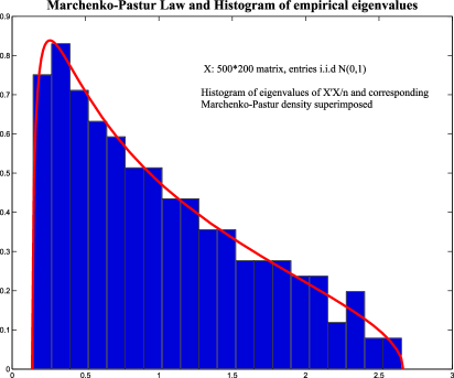
Figure 1: Illustration of Marčenko–Pastur-law, $n=500$, $p=200$. The red curve is the density of the Marčenko–Pastur-law for $\rho=2/5$. The simulation was done with i.i.d. Gaussian data. The histogram is the histogram of eigenvalues of $X^{\prime}X/n$.

What is striking about this result is that it implies that the largest eigenvalue of $\Sigma$, $\lambda_{1}$, will be overestimated by $l_{1}$ the largest eigenvalue of $\hat{\Sigma}$. Also, the smallest eigenvalue of $\Sigma$, $\lambda_{p}$, will be underestimated by the smallest eigenvalue of $\hat{\Sigma}$, $l_{p}$. As a matter of fact, in the model described above, $\Sigma$ has all its eigenvalues equal to 1, so $\lambda_{1}(\Sigma)=\lambda_{p}(\Sigma)=1$, while $l_{1}$ will asymptotically be larger or equal to $(1+\sqrt{\rho})^{2}$ and $l_{p}$ smaller or equal to $(1-\sqrt{\rho})^{2}$ (in the Gaussian case and several others, $l_{1}$ and $l_{p}$ converge to those limits). We note that the result of Marčenko and Pastur (1967) is not limited to the case where $\Sigma$ is identity, as presented here, but holds for general covariance $\Sigma$ ($F_{p}$ has of course a different limit then).

Perhaps more concretely, let us consider a projection of the data along a vector $v$, with $\|v\|_{2}=1$, where $\|v\|_{2}$ is the Euclidian norm of $v$. Here it is clear that, if $X\sim{\cal N}(0,\mathrm{Id}_{p})$, $\operatorname{var}(v^{\prime}X)=1$, for all $v$, since $v^{\prime}X\sim{\cal N}(0,1)$. However, if we do not know $\Sigma$ and estimate it by $\hat{\Sigma}$, a naive (and wrong) reasoning suggests that we can find direction of lower variance than 1, namely those corresponding to eigenvectors of $\hat{\Sigma}$ associated with eigenvalues that are less than 1. In particular, if $v_{p}$ is the eigenvector associated with $l_{p}$, the smallest eigenvalue of $\hat{\Sigma}$, by naively estimating, for $X$ independent of $\{X_{i}\}_{i=1}^{n}$, the variance in the direction of $v_{p}$, $\operatorname{var}(v_{p}^{\prime}X)$, by the empirical version $v_{p}^{\prime}\hat{\Sigma}v_{p}$, one would commit a severe mistake: the variance in any direction is 1, but it would be estimated by something roughly equal to $(1-\sqrt{p/n})^{2}$ in the direction of $v_{p}$.

In a portfolio optimization context, this suggests that by using standard estimators, such as the sample covariance matrix, when solving the high-dimensional Markowitz problem, one might underestimate the variance of certain portfolios (or “optimal” vectors of weights). As a matter of fact, in the previous toy example, thinking (wrongly) that there is low variance in the direction $v_{p}$, one might (numerically) “load” this direction more than warranted, given that the true variance is the same in all directions.

This simple argument suggests that severe problems might arise in the high-dimensional Markowitz problem and other quadratic programs with linear constraints, and in particular, risk might be underestimated. While this heuristic argument is probably clear to specialists of random matrix theory, the problem had not been investigated at a mathematical level of rigor in that literature before this paper was submitted [the paper Bai, Liu and Wong (2009) has appeared while this paper was being refereed. It is concerned with different models than the ones we will be investigating and our results do not overlap]. It has received some attention at a physical level of rigor [see, e.g., Pafka and Kondor (2003), where the authors treat only the Gaussian case, and do not investigate the effect of the mean, which as we show below creates problems of its own]. In this paper, we propose a theoretical analysis of the problem in a Gaussian and elliptical framework for general quadratic programs with linear constraints, one of them involving the parameter $\mu$. Our results and contributions are several-fold. We relate the empirical efficient frontier to the theoretical efficient frontier that is key to the Markowitz theory, in a variety of theoretical settings. We show that the empirical frontier generally yields an underestimation of the risk of the portfolio and that Gaussian analysis gives an over-optimistic view of this problem. We show that the expected returns of the naive “optimal” portfolio are poorly estimated by $\mu_{P}$. We argue that the bootstrap will not solve the problems we are pointing out here. Beside new formulas, we also provide robust estimators of the various quantities we are interested in.

The paper is divided into four main parts and a conclusion. In Section 2, to make the paper self-contained, we discuss the solution of quadratic problems with linear equality constraints—a focus of this paper. In Section 3, we study the impact of parameter estimation on the solution of these problems when the observed data is i.i.d. Gaussian and obtain some exact distributional results for fixed $p$ and $n$. In Section 4, we obtain results in the case where the data is elliptically distributed. This allows us also to understand the impact of correlation between observations in the Gaussian case and to get information about the behavior of the nonparametric bootstrap. In Section 5, we apply the results of Section 4 to the quadratic programs at hand and compare the elliptical and the Gaussian cases. We show, among other things, that the Gaussian results are not robust in the class of elliptical distribution. In particular, two models may yield the same $\mu$ and $\Sigma$ but can have very different empirical behavior. In Section 5, we also propose various schemes to correct the problems we highlight (see pages 2, 3 and 4 for pictures) and study more general problems with linear constraints (see Section 5.6). The conclusion summarizes our findings and the Appendix contains various facts and proofs that did not naturally flow in the main text or were better highlighted by being stated separately.

Several times in the paper $\hat{\Sigma}^{-1}$ and $\Sigma^{-1}$ will appear. Unless otherwise noted, when taking the inverse of a population matrix, we implicitly assume that it exists. The question of existence of inverse of sample covariance matrices is well understood in the statistics literature. Because our models will have a component with a continuous distribution, there are essentially no existence problems (unless we explicitly mention and treat them) as proofs similar to standard ones found in textbooks [e.g., Anderson (2003)] would show. Hence, we do not belabor this point any further in the rest of the paper as our focus is on things other than rather well-understood technical details, and the paper is already a bit long.

Finally, let us mention that while the Finance motivation for our study is important to us, we treat the problem in this paper as a high-dimensional $M$-estimation question (which we think has practical relevance). We will not introduce particular modelization assumptions which might be relevant for practitioners of Finance but might make the paper less relevant in other fields. A companion paper (El Karoui, 2009b) deals with more “financial” issues and the important question of the realized risk of portfolios that are “plug-in” solutions of the Markowitz problem.

2 Quadratic programs with linear equality constraints

We discuss here the properties of the solution of quadratic programs with linear equality constraints as they lay the foundations for our analysis of similar problems involving estimated parameters (and of problems with inequality constraints). We included this section for the convenience of the reader to make the paper as self-contained as possible.

The problem we want to solve is the following:

$$\cases{\displaystyle\min_{w\in\mathbb{R}^{p}}\frac{1}{2}w^{\prime}\Sigma w,\cr\displaystyle w^{\prime}v_{i}=u_{i},\qquad 1\leq i\leq k.}$$ (QP-eqc)

Here $\Sigma$ is a positive definite matrix of size $p\times p$, $v_{i}\in\mathbb{R}^{p}$ and $u_{i}\in\mathbb{R}$. We have the following theorem:

Theorem 2.1

Let us call $V$ the $p\times k$ matrix whose $i$th column is $v_{i}$, $U$ the $k$ dimensional vector whose $i$th entry is $u_{i}$ and $M$ the $k\times k$ matrix

$$M=V^{\prime}\Sigma^{-1}V.$$

We assume that the $v_{i}$’s are such that $M$ is invertible. The solution of the quadratic program with linear equality constraints (QP-eqc) is achieved for

$$w_{\mathrm{optimal}}=\Sigma^{-1}VM^{-1}U,$$

and we have

$$w_{\mathrm{optimal}}^{\prime}\Sigma w_{\mathrm{optimal}}=U^{\prime}M^{-1}U.$$

Let us call $\lambda$ a $k$ dimensional vector of Lagrange multipliers. The Lagrangian function is, in matrix notation,

$$L(w,\lambda)=\frac{w^{\prime}\Sigma w}{2}-\lambda^{\prime}(V^{\prime}w-U).$$

This is clearly a (strictly) convex function in $w$, since $\Sigma$ is positive definite by assumption. We have

$$\frac{\partial L}{\partial w}=\Sigma w-V\lambda.$$

So $w_{\mathrm{optimal}}=\Sigma^{-1}V\lambda$. Now we know that $U=V^{\prime}w_{\mathrm{optimal}}$. So $U=V^{\prime}\Sigma^{-1}V\lambda=M\lambda$. Therefore,

$$w_{\mathrm{optimal}}=\Sigma^{-1}VM^{-1}U.$$

We deduce immediately that

$$w_{\mathrm{optimal}}^{\prime}\Sigma w_{\mathrm{optimal}}=U^{\prime}M^{-1}U.$$

We now turn to another result which will prove to be useful later. It gives a compact representation of linear combinations of the weights of the optimal solution, and we will rely heavily on it in particular in the case of Gaussian data.

Lemma 2.2

Let us consider $w_{\mathrm{optimal}}$ the solution of the optimization problem (QP-eqc). Let $\gamma$ be a vector in $\mathbb{R}^{p}$. Let us call ${\cal M}$ the $(k+1)\times(k+1)$ matrix that is written in block form

$${\cal M}=\pmatrix{V^{\prime}\Sigma^{-1}V&V^{\prime}\Sigma^{-1}\gamma\cr\gamma^{\prime}\Sigma^{-1}V&\gamma^{\prime}\Sigma^{-1}\gamma}.$$

Assume that ${\cal M}$ is invertible. Then

$$\gamma^{\prime}w_{\mathrm{optimal}}=-\frac{1}{{\cal M}^{-1}_{k+1,k+1}}(U^{\prime}0){\cal M}^{-1}\pmatrix{0_{k}\cr 1}.$$ (1)

The proof is a consequence of the results discussed in the Appen- dix concerning inverses of partitioned matrices [see Section A.1 and equation (A.4) there]. Let us write

$${\cal M}=\pmatrix{{\cal M}_{11}&{\cal M}_{12}\cr{\cal M}_{21}&{\cal M}_{22}},$$

where ${\cal M}_{11}$ is $k\times k$, ${\cal M}_{12}$ is naturally $k\times 1$ and ${\cal M}_{22}$ is a scalar. With the same block notation, we have

$${\cal M}^{-1}=\pmatrix{{\cal M}^{11}&{\cal M}^{12}\cr{\cal M}^{21}&{\cal M}^{22}}.$$

Then, we know [see equation (A.4)] that ${\cal M}^{12}=-{\cal M}_{11}^{-1}{\cal M}_{12}{\cal M}^{22},$ but since ${\cal M}^{22}$ is a scalar, equal to ${\cal M}^{-1}(k+1,k+1)$, we have

$${\cal M}_{11}^{-1}{\cal M}_{12}=-{\cal M}^{12}/{\cal M}^{22}.$$

Now ${\cal M}_{11}^{-1}{\cal M}_{12}=(V^{\prime}\Sigma^{-1}V)^{-1}V^{\prime}\Sigma^{-1}\gamma$, so $U^{\prime}{\cal M}_{11}^{-1}{\cal M}_{12}=w_{\mathrm{optimal}}^{\prime}\gamma$. Hence,

$$w_{\mathrm{optimal}}^{\prime}\gamma=-\frac{1}{{\cal M}^{22}}(U^{\prime}0){\cal M}^{-1}\pmatrix{0_{k}\cr 1}.$$

We note that here $({\cal M}^{22})^{-1}=\gamma^{\prime}\Sigma^{-1}\gamma-\gamma^{\prime}\Sigma^{-1}VM^{-1}V^{\prime}\Sigma^{-1}\gamma$, as an application of equation (A.2) clearly shows.

3 QP with equality constraints: Impact of parameter estimation in the Gaussian case

From now on, we will assume that we are in the high-dimensional setting where $p$ and $n$ go to infinity. Our study will be divided into two. We will first consider the Gaussian setting (in this section) and then study an elliptical distribution setting (in Section 4). (We note that for the Markowitz problem, the assumption of Gaussianity would be satisfied if we worked under Black–Scholes diffusion assumptions for our assets and were considering log-returns as our observations.) Interestingly, we will show that the results are not robust against the assumption of Gaussianity, which is not (so) surprising in light of recent random matrix results [see El Karoui (2009a)]. We will also show that understanding the elliptical setting allows us to understand the impact of correlation between observations and to discuss bootstrap-related ideas. In particular, we will see that various problems arise with the bootstrap in high-dimension and that the results change when one deals with observations that are correlated (in time) or not.

We also address similar questions concerning inequality constrained problems in Section 5.6.

Before we proceed, we need to set up some notations: we call $\mathbf{e}$ the $p$-dimensional vector whose entries are all equal to 1. We call $V$, as above, the matrix containing all of our constraint vectors, which we may have to estimate (for instance, if $v_{i}=\mu$ for a certain $i$). We call $\widehat{V}$ the matrix of estimated constraint vectors.

The template question for all our investigations will be the following (Markowitz) question: what can be said of the statistical properties of the solution of

$$\cases{\displaystyle\min_{w\in\mathbb{R}^{p}}w^{\prime}\hat{\Sigma}w,\cr\displaystyle w^{\prime}\hat{\mu}=\mu_{P},\cr\displaystyle w^{\prime}\mathbf{e}=1}$$

compared to the solution of the population version

$$\cases{\displaystyle\min_{w\in\mathbb{R}^{p}}w^{\prime}\Sigma w,\cr\displaystyle w^{\prime}\mu=\mu_{P},\cr\displaystyle w^{\prime}\mathbf{e}=1?}$$

We will solve the problem at a much greater degree of generality, by considering first quadratic programs with linear equality constraints (see Section 5.6 for inequality constraints) and comparing the solutions of

$$\cases{\displaystyle\min_{w\in\mathbb{R}^{p}}w^{\prime}\hat{\Sigma}w,\cr\displaystyle w^{\prime}v_{i}=u_{i},\qquad 1\leq i\leq k-1,\cr\displaystyle w^{\prime}\hat{\mu}=u_{k}}$$ (QP-eqc-Emp)

and

$$\cases{\displaystyle\min_{w\in\mathbb{R}^{p}}w^{\prime}\Sigma w,\cr\displaystyle w^{\prime}v_{i}=u_{i},\qquad 1\leq i\leq k-1,\cr\displaystyle w^{\prime}\mu=u_{k}.}$$ (QP-eqc-Pop)

Here $\hat{\Sigma}$ and $\hat{\mu}$ will be estimated from the data. We call $w_{\mathrm{emp}}$ the vector that yields a solution of problem (QP-eqc-Emp) and $w_{\mathrm{theo}}$ the vector that yields a solution of problem (QP-eqc-Pop).

We call $\widehat{V}$ the $p\times k$ matrix containing $\{v_{i}\}_{i=1}^{k-1}$ and $\hat{\mu}$, and $V$ its population counterpart, which contains $\{v_{i}\}_{i=1}^{k-1}$ and $\mu$. We assume that $\{v_{i}\}_{i=1}^{k-1}$ are deterministic and known (just like the vector $\mathbf{e}$ in the Markowitz problem). In our analysis, $k$ will be held fixed. (The $k$th column of $\widehat{V}$ will contain $\hat{\mu}$ in general or our estimator of $\mu$.)

As should be clear from Theorem 2.1, the properties of the entries of the matrix $\widehat{V}^{\prime}\hat{\Sigma}^{-1}\widehat{V}$ as compared to those of the matrix $V^{\prime}\Sigma^{-1}V$ will be key to our understanding of this question. In what follows, we assume that the vectors $\hat{v}_{i}$ are either deterministic or equal to $\hat{\mu}$. The extension to linear combinations of a deterministic vector and $\hat{\mu}$ is straightforward. We also note that in the Gaussian case, we could just assume that the $\hat{v}_{i}$ are (deterministic) functions of $\hat{\mu}$ (because $\hat{\mu}$ and $\hat{\Sigma}$ are independent in this case). On the other hand, the vector $U$ is assumed to be deterministic.

Before we proceed, let us mention that after our study was completed, we learned of similar results (restricted to the Markowitz case and not dealing with general quadratic programs with linear equality constraints) by Kan and Smith (2008). We stress the fact that our work was independent of theirs and is more general which is why it is included in the paper.

3.1 Efficient frontier problems

We first study questions concerning the efficient frontier and then turn to information we can get about linear functionals of the empirical weights.

Theorem 3.1

Let us assume that we observe data $X_{i}\stackrel{{\scriptstyle i.i.d.}}{{\backsim}}{\cal N}(\mu,\Sigma)$, for $i=1,\ldots,n$. Here $\Sigma$ is $p\times p$ and $p<n$. Suppose we estimate $\Sigma$ with the sample covariance matrix $\hat{\Sigma}$, and $\mu$ with the sample mean $\hat{\mu}$. Suppose we wish to solve the problem

$$\cases{\displaystyle\min_{w\in\mathbb{R}^{p}}w^{\prime}\Sigma w,\cr\displaystyle w^{\prime}v_{j}=u_{j},\qquad 1\leq j\leq k.}$$ (QP-eqc-Pop)

where $u_{j}$ are deterministic, $v_{j}$ are deterministic and given for $j<k$ and $v_{k}=\mu$. Assume that we use as a proxy for the previous problem the empirical version with plugged-in parameters. Let us consider the solution of the problem

$$\cases{\displaystyle\min_{w\in\mathbb{R}^{p}}w^{\prime}\hat{\Sigma}w,\cr\displaystyle w^{\prime}\hat{v}_{j}=u_{j},\qquad 1\leq j\leq k.}$$ (QP-eqc-Emp)

Now $\hat{v}_{j}=v_{j}$ for $j<k$ and $\hat{v}_{k}=f(\hat{\mu})$, for a given deterministic function $f$. Let us call $w_{\mathrm{emp}}$ the corresponding “weight” vector. The plug-in estimate of $w^{\prime}\Sigma w$ is $w_{\mathrm{emp}}^{\prime}\hat{\Sigma}w_{\mathrm{emp}}$. Let us call $w_{\mathrm{oracle}}$ the optimal solution of the quadratic program obtained under the assumption that $\Sigma$ is given, but $\mu$ is not and is estimated by $f(\hat{\mu})$. Finally, we assume that $n-1-p+k>0$.

Then we have

$$w_{\mathrm{emp}}^{\prime}\hat{\Sigma}w_{\mathrm{emp}}=w_{\mathrm{oracle}}^{\prime}\Sigma w_{\mathrm{oracle}}\frac{\chi^{2}_{n-1-p+k}}{n-1},$$ (2)

where $w_{\mathrm{oracle}}^{\prime}\Sigma w_{\mathrm{oracle}}$ is random (because $\hat{\mu}$ is) but is statistically independent of $\chi^{2}_{n-1-p+k}$. Also,

$$w_{\mathrm{oracle}}^{\prime}\Sigma w_{\mathrm{oracle}}=U^{\prime}(\widehat{V}^{\prime}\Sigma^{-1}\widehat{V})^{-1}U.$$

The previous theorem means that the cost of not knowing the covariance matrix and estimating it is the apparition of the $\frac{\chi^{2}_{n-1-p+k}}{n-1}$. In the high-dimensional setting when $p$ and $n$ are of the same order of magnitude and $n-p$ is large, this terms is approximately $1-(p-k)/(n-1)$. Hence, the theorem quantifies the random matrix intuition that having to estimate the high-dimensional covariance matrix at stake here leads to risk underestimation, by the factor $1-(p-k)/(n-1)$. In other words, using plug-in procedures leads to over-optimistic conclusions in this situation.

We also note that the previous theorem shows that, in the Gaussian setting under study here, the effect of estimating the mean and the covariance on the solution of the quadratic program are “separable”: the effect of the mean estimation is in the oracle term, while the effect of estimating the covariance is in the $\chi^{2}_{n-p-1+k}/(n-1)$ term. To show risk underestimation, it will therefore be necessary to relate $w_{\mathrm{oracle}}^{\prime}\Sigma w_{\mathrm{oracle}}$ to $w_{\mathrm{theo}}^{\prime}\Sigma w_{\mathrm{theo}}$. We do it in Proposition 3.2 but first give a proof of Theorem 3.1.

Proof of Theorem 3.1 The crux of the proof is the following result, which is well known by statisticians, concerning (essentially) blocks of the inverse of a Wishart matrix: if $S\sim\cal{W}_{p}(\Sigma,m)$, that is, $S$ is a $p\times p$ Wishart matrix with $m$ degree of freedoms and covariance $\Sigma$, and $A$ is $p\times k$, deterministic matrix, then, when $m>p$,

$$(A^{\prime}S^{-1}A)^{-1}\sim\cal{W}_{k}\bigl{(}(A^{\prime}\Sigma^{-1}A)^{-1},m-p+k\bigr{)}.$$

We refer to Eaton [(1983), Proposition 8.9, page 312] for a proof, and to Mardia, Kent and Bibby [(1979), pages 70–73] for related results.

Another important remark is the well-known fact that, in the situation we are considering, $\hat{\mu}$ is ${\cal N}(\mu,\Sigma/n)$ and independent of $\hat{\Sigma}$. Finally, it is also well known that if $S\sim\cal{W}_{p}(\Sigma,m)$ and $U$ is a $p$-dimensional deterministic vector, then $U^{\prime}SU=U^{\prime}\Sigma U\chi^{2}_{m}$.

Now $\hat{\Sigma}\sim\cal{W}_{p}(\Sigma,n-1)/(n-1)$. Therefore, since $\widehat{V}$ is a function of $\hat{\mu}$, we have, by independence of $\hat{\mu}$ and $\hat{\Sigma}$,

$$(\widehat{V}^{\prime}\hat{\Sigma}^{-1}\widehat{V})^{-1}|\hat{\mu}\sim\cal{W}_{k}\bigl{(}(\widehat{V}^{\prime}\Sigma^{-1}\widehat{V})^{-1},n-1-p+k\bigr{)}/(n-1).$$

Therefore,

$$\frac{U^{\prime}(\widehat{V}^{\prime}\hat{\Sigma}^{-1}\widehat{V})^{-1}U}{U^{\prime}(\widehat{V}^{\prime}\Sigma^{-1}\widehat{V})^{-1}U}\bigg{|}\hat{\mu}\sim\frac{\chi^{2}_{n-p-1+k}}{n-1}.$$

Because the right-hand side does not depend on $\hat{\mu}$, we have established the independence of

$$\frac{U^{\prime}(\widehat{V}^{\prime}\hat{\Sigma}^{-1}\widehat{V})^{-1}U}{U^{\prime}(\widehat{V}^{\prime}\Sigma^{-1}\widehat{V})^{-1}U}\quad\mbox{and}\quad\frac{\chi^{2}_{n-p-1+k}}{n-1}.$$

Hence, we conclude that

$$U^{\prime}(\widehat{V}^{\prime}\hat{\Sigma}^{-1}\widehat{V})^{-1}U=U^{\prime}(\widehat{V}^{\prime}\Sigma^{-1}\widehat{V})^{-1}U\frac{\chi^{2}_{n-p-1+k}}{n-1},$$

and the two terms are independent. Now the term $U^{\prime}(\widehat{V}^{\prime}\Sigma^{-1}\widehat{V})^{-1}U$ is the estimate we would get for the solution of problem (QP-eqc-Pop), if $\Sigma$ were known and $\mu$ were estimated by $f(\hat{\mu})$. In other words, it is the “oracle” solution described above.

3.1.1 Some remarks on the oracle solution

Theorem 3.1 sheds light on the separate effects of mean and covariance estimation on the problem considered above. To understand further the problem of risk estimation, we need to better understand the role the estimation of the mean might play. This is what we do now.

Proposition 3.2.

Suppose that the last column of $\widehat{V}$ is $\hat{\mu}$. Let us call $V_{-k}$ the $p\times k-1$ dimensional matrix whose $j$th column is $v_{j}$, which are known deterministic vectors. Suppose that $M=V^{\prime}\Sigma^{-1}V=\mathrm{O}(1)$. Suppose further that $\lambda_{k}(V^{\prime}\Sigma^{-1}V)\gg n^{-1/2}$, where $\lambda_{k}(S)$ is the smallest eigenvalue of the $k\times k$ matrix $S$.

Further, call $M=V^{\prime}\Sigma^{-1}V\in\mathbb{R}^{k\times k}$ and call $e_{i}$ the canonical basis vectors in $\mathbb{R}^{k}$. Finally, call $\alpha=\chi^{2}_{p}/n$.

Then, when $p/n\rightarrow\rho\in(0,1)$, asymptotically,

$$w_{\mathrm{oracle}}^{\prime}\Sigma w_{\mathrm{oracle}}=w_{\mathrm{theo}}^{\prime}\Sigma w_{\mathrm{theo}}-\alpha\frac{(U^{\prime}M^{-1}e_{k})^{2}}{1+\alpha e_{k}^{\prime}M^{-1}e_{k}}+\mathrm{o}_{P}(w_{\mathrm{theo}}^{\prime}\Sigma w_{\mathrm{theo}}).$$

Let us discuss a little bit this result before we provide a proof. In the asymptotics we have in mind and are considering, $p/n\rightarrow\rho\in(0,1)$ and therefore $\alpha\simeq p/n+\mathrm{O}(n^{-1/2})$. So if $\delta_{n}=(U^{\prime}M^{-1}e_{k})^{2}/(1+p/ne_{k}^{\prime}M^{-1}e_{k})$, when the above analysis applies, the impact of the estimation of $\mu$ by $\hat{\mu}$ will be risk underestimation, just as is the case for the case of the covariance matrix. Here, we can also quantify the impact of this estimation of $\mu$ by $\hat{\mu}$: it leads to risk underestimation by the amount $\alpha\delta_{n}$.

Proof of Proposition 3.2 Let us write $\hat{\mu}=\mu+e$, where $e\sim{\cal N}(0,\Sigma/n)$. Clearly, $e=n^{-1/2}\Sigma^{1/2}Z$, where $Z$ is ${\cal N}(0,\mathrm{Id}_{p})$. We have, using block notations,

$$\widehat{V}^{\prime}\Sigma^{-1}\widehat{V}=V^{\prime}\Sigma^{-1}V+\pmatrix{0&0\cr 0&e^{\prime}\Sigma^{-1}e}+\pmatrix{0&V_{-k}^{\prime}\Sigma^{-1}e\cr e^{\prime}\Sigma^{-1}V_{-k}&2\mu^{\prime}\Sigma^{-1}e}.$$

Replacing $e$ by its value, we have $\mu^{\prime}\Sigma^{-1}e\sim{\cal N}(0,\mu^{\prime}\Sigma^{-1}\mu/n)$. By the same token, we can also get that

$$V_{-k}^{\prime}\Sigma^{-1}e=\frac{1}{\sqrt{n}}V_{-k}^{\prime}\Sigma^{-1/2}Z\sim{\cal N}\biggl{(}0,\frac{V_{-k}^{\prime}\Sigma^{-1}V_{-k}}{n}\biggr{)}.$$

Our assumption that $V^{\prime}\Sigma^{-1}V=\mathrm{O}(1)$ implies that $\mu^{\prime}\Sigma^{-1}\mu=\mathrm{O}(1)$ and $V_{-k}^{\prime}\times\Sigma^{-1}V_{-k}=\mathrm{O}(1)$. Therefore,

$$\pmatrix{0&V_{-k}^{\prime}\Sigma^{-1}e\cr e^{\prime}\Sigma^{-1}V_{-k}&2\mu^{\prime}\Sigma^{-1}e}=\mathrm{O}_{P}\biggl{(}\frac{1}{\sqrt{n}}\biggr{)}.$$

Hence, since $e^{\prime}\Sigma^{-1}e=Z^{\prime}Z/n=\alpha$,

$$\widehat{V}^{\prime}\Sigma^{-1}\widehat{V}=V^{\prime}\Sigma^{-1}V+\alpha e_{k}e_{k}^{\prime}+\mathrm{O}_{P}(n^{-1/2}).$$

Our assumptions guarantee that $\lambda_{k}(V^{\prime}\Sigma^{-1}V)\gg n^{-1/2}$, and therefore$\lambda_{k}(V^{\prime}\Sigma^{-1}\times V+\alpha e_{k}e_{k}^{\prime})\gg n^{-1/2}$. In other respects, let $A$ be a matrix such that $\lambda_{p}(A)\gg n^{-1/2}$ and $E$ be a matrix such that $E=\mathrm{O}(n^{-1/2})$. Recall that for symmetric matrices, $\lambda_{p}(A+E)\geq\lambda_{p}(A)+\lambda_{p}(E)$ [see, e.g., Weyl’s theorem, Horn and Johnson (1994), page 185]. So in this situation, $(A+E)^{-1}=\mathrm{o}(n^{1/2})$. Let us now consider the implications of this remark on the difference of $(A+E)^{-1}$ and $A^{-1}$. We claim that $(A+E)^{-1}=A^{-1}+\mathrm{o}(A^{-1})$. By the first resolvent identity, $(A+E)^{-1}=A^{-1}-(A+E)^{-1}EA^{-1}$; our previous remark implies that $\sigma_{1}[(A+E)^{-1}E]=\mathrm{o}(1)$ and the result follows. Applying the results of this discussion to $A=V^{\prime}\Sigma^{-1}V+\alpha e_{k}e_{k}^{\prime}$ and $A+E=\widehat{V}^{\prime}\Sigma^{-1}\widehat{V}$, we have

$$\widehat{V}^{\prime}\Sigma^{-1}\widehat{V}=(V^{\prime}\Sigma^{-1}V+\alpha e_{k}e_{k}^{\prime})^{-1}+\mathrm{o}_{P}\bigl{(}(V^{\prime}\Sigma^{-1}V+\alpha e_{k}e_{k}^{\prime})^{-1}\bigr{)}.$$

We can now use well-known results concerning inverses of rank-1 perturbation of matrices, namely

$$(V^{\prime}\Sigma^{-1}V+\alpha e_{k}e_{k}^{\prime})^{-1}=(M+\alpha e_{k}e_{k}^{\prime})^{-1}=M^{-1}-\alpha\frac{M^{-1}e_{k}e_{k}^{\prime}M^{-1}}{1+\alpha e_{k}^{\prime}M^{-1}e_{k}}.$$

This allows us to conclude that

$$U^{\prime}(\widehat{V}^{\prime}\Sigma^{-1}\widehat{V})^{-1}U=U^{\prime}M^{-1}U-\alpha\frac{(U^{\prime}M^{-1}e_{k})^{2}}{1+\alpha e_{k}^{\prime}M^{-1}e_{k}}+\mathrm{o}_{P}(U^{\prime}M^{-1}U).$$

This is the result announced in the theorem and the proof is complete.

We can now combine the results of Theorem 3.1 and Proposition 3.2 to obtain the following corollary.

Corollary 3.3.

We assume that the assumptions of Theorem 3.1 and Proposition 3.2 hold and that $p/n$ has a finite nonzero limit, as $n\rightarrow\infty$, and $n-p$ tends to infinity. Then we have

$$w_{\mathrm{emp}}^{\prime}\hat{\Sigma}w_{\mathrm{emp}} = \biggl{(}1-\frac{p-k}{n-1}\biggr{)}\biggl{(}w_{\mathrm{theo}}^{\prime}\Sigma w_{\mathrm{theo}}-\frac{p}{n}\frac{(U^{\prime}M^{-1}e_{k})^{2}}{1+({p}/{n})e_{k}^{\prime}M^{-1}e_{k}}\biggr{)}$$

$${}+\mathrm{o}_{P}(w_{\mathrm{theo}}^{\prime}\Sigma w_{\mathrm{theo}}\vee n^{-1/2}),$$

where $M$ is the population quantity $M=V^{\prime}\Sigma^{-1}V$.

The corollary shows that the effects of both covariance and mean estimation are to underestimate the risk, and the empirical frontier is asymptotically deterministic.

3.2 On the optimal weights

Our matrix characterization of the empirical optimal weights (Lemma 2.2) allows us to give a precise characterization of the statistical properties of linear functionals of these weights. We give here some exact results, concerning distributions and expectations of those functionals. A longer discussion, including robustness and more detailed bias issues can be found in Section 5.

Proposition 3.4.

Assume that the assumptions of Theorem 3.1 hold and in particular $X_{i}$ are i.i.d. ${\cal N}(\mu,\Sigma_{p})$. Let $\gamma$ be a fixed $n$-dimensional vector. Let us call $\widehat{V}_{\gamma}=(\widehat{V}\gamma)$ the $p\times(k+1)$ matrix whose first $k$ columns are those of $\widehat{V}$. Let $\widehat{N}_{\gamma}=(\widehat{V}_{\gamma}^{\prime}\Sigma^{-1}\widehat{V}_{\gamma})^{-1}$ and $W_{\gamma}$ be a $(k+1)\times(k+1)$ matrix with distribution $\cal{W}_{k+1}(\widehat{N}_{\gamma},n-p+k)$ (conditional on $\hat{\mu}$). Then,

$$\gamma^{\prime}w_{\mathrm{emp}}|\hat{\mu}\stackrel{{\scriptstyle{\cal L}}}{{=}}-\frac{\sum_{i=1}^{k}u_{i}W_{\gamma}(i,k+1)}{W_{\gamma}(k+1,k+1)}.$$

In particular,

$$\mathbf{E}(\gamma^{\prime}w_{\mathrm{emp}}|\hat{\mu})=-\frac{\sum_{i=1}^{k}u_{i}\widehat{N}_{\gamma}(i,k+1)}{\widehat{N}_{\gamma}(k+1,k+1)}.$$

We note, somewhat heuristically, that when $\mu$ is estimated by $\hat{\mu}$, since $\hat{\mu}\sim{\cal N}(\mu,\Sigma/n)$, $\hat{\mu}^{\prime}\Sigma^{-1}\hat{\mu}\simeq\mu^{\prime}\Sigma^{-1}\mu+p/n$, when $p$, $n$ and $n-p$ are all large (we refer again to Section 5 for a more precise statement). Hence $\widehat{N}_{\gamma}$ is a not a consistent estimator of $N_{\gamma}=(V_{\gamma}^{\prime}\Sigma^{-1}V_{\gamma})^{-1}$. As we will see in Section 5.2 and as can be expected from the previous proposition, this will also imply bias for linear combinations of empirical optimal weights. We will show in particular that returns are overestimated when using $\hat{\mu}$ as an estimator for $\mu$.

Another interesting aspect of the previous proposition is that it allows us to understand the fluctuation behavior of $\gamma^{\prime}w_{\mathrm{emp}}$ when $n-p+k$ is large: as a matter of fact, the limiting fluctuation behavior of the entries of a (fixed-dimensional) Wishart matrix with large number of degrees of freedom is well known [see, e.g., Anderson (2003), Theorem 3.4.4, page 87] and the $\delta$-method can be applied to get the information—conditional on $\hat{\mu}$.

For instance, if we assume that, conditional on $\hat{\mu}$, the matrix $\widehat{N}_{\gamma}$ converges to a matrix $N^{0}_{\gamma}$, which possibly depends on $\hat{\mu}$, we see that calling $\nu$ the last column $W_{\gamma}/(n-p+k)$, $\nu$ is asymptotically normal (all statements are conditional on $\hat{\mu}$), if $n-p+k$ goes to infinity when $p$ and $n$ go to infinity. Furthermore we know the limiting covariance of $\nu$ (after scaling by $\sqrt{n-p+k}$), using Theorem 3.4.4 in Anderson (2003). Let us call it $\Gamma_{0}$ and let us call $\nu_{0}$ the limit of $\nu$—which we assume exists.

If we assume that $\nu_{0}(k+1)$ is not 0, Slutsky’s lemma and the $\delta$-method give us through simple computations that

$$\sqrt{n-p+k}\biggl{(}\gamma^{\prime}w_{\mathrm{emp}}+\frac{\sum_{i=1}^{k}u_{i}\nu_{0}(i)}{\nu_{0}(k+1)}\biggr{)}\Big{|}\hat{\mu}\Longrightarrow\frac{1}{\nu_{0}(k+1)^{2}}{\cal N}(0,C^{\prime}\Gamma_{0}C),$$

where $C=\nu_{0}(k+1){U\choose 0}-({U\choose 0}^{\prime}\nu_{0})e_{k+1}$.

We know the distribution of $\hat{\mu}$, so we could get (limiting) unconditional results for $\gamma^{\prime}w_{\mathrm{emp}}$. This is not hard but a bit tedious if we want explicit expressions, and because our focus is mostly on first-order properties in this paper, we do not state the result.

Proof of Proposition 3.4 The proof follows from the representation we gave in Lemma 2.2, that is,

$$\gamma^{\prime}w_{\mathrm{emp}}=-\frac{1}{(\widehat{V}_{\gamma}^{\prime}\hat{\Sigma}^{-1}\widehat{V}_{\gamma})^{-1}(k+1,k+1)}(U^{\prime}0)(\widehat{V}_{\gamma}^{\prime}\hat{\Sigma}^{-1}\widehat{V}_{\gamma})^{-1}\pmatrix{0_{k}\cr 1},$$

and the fact that, by the same arguments as before, conditional on $\hat{\mu}$,

$$(\widehat{V}_{\gamma}^{\prime}\hat{\Sigma}^{-1}\widehat{V}_{\gamma})^{-1}|\hat{\mu}\sim\cal{W}_{k+1}\bigl{(}(\widehat{V}_{\gamma}^{\prime}\Sigma^{-1}\widehat{V}_{\gamma})^{-1},n-p+k\bigr{)}/(n-1).$$

We conclude that

$$\gamma^{\prime}w_{\mathrm{emp}}|\hat{\mu}\stackrel{{\scriptstyle{\cal L}}}{{=}}-\frac{(U^{\prime}0)W_{\gamma}{0_{k}\choose 1}}{W_{\gamma}(k+1,k+1)}=-\frac{\sum_{i=1}^{k}u_{i}W_{\gamma}(i,k+1)}{W_{\gamma}(k+1,k+1)}.$$

This shows the fist part of the proposition.

The second part follows from the following observation. Suppose the matrix $P$ is $\cal{W}_{p}(\mathrm{Id}_{p},K)$. If $\alpha$ and $\beta$ are $n$-dimensional, orthogonal vectors, let us consider

$$\frac{\alpha^{\prime}P\beta}{\beta^{\prime}P\beta}.$$

We can, of course, write $P=\sum_{i=1}^{K}Y_{i}Y_{i}^{\prime}$, where $Y_{i}$ are i.i.d. ${\cal N}(0,\mathrm{Id}_{p})$. In other respects, $Y_{i}^{\prime}\alpha$ and $Y_{i}^{\prime}\beta$ are clearly independent normal random variables, since their covariance is $\alpha^{\prime}\beta=0$, and they are normal. So

$$\mathbf{E}\biggl{(}\frac{\alpha^{\prime}P\beta}{\beta^{\prime}P\beta}\Big{|}\{Y_{i}^{\prime}\beta\}_{i=1}^{K}\biggr{)}=0$$

because the quantity whose expectation we are taking is a linear combination of mean 0 independent normal random variables. Hence, also,

$$\mathbf{E}\biggl{(}\frac{\alpha^{\prime}P\beta}{\beta^{\prime}P\beta}\biggr{)}=0.$$

Now, when $\alpha$ is not orthogonal to $\beta$, we write $\alpha=\beta(\alpha^{\prime}\beta)/\|\beta\|_{2}^{2}+\delta$, where $\delta$ is orthogonal to $\beta$. We immediately deduce that in general,

$$\mathbf{E}\biggl{(}\frac{\alpha^{\prime}P\beta}{\beta^{\prime}P\beta}\biggr{)}=\frac{\alpha^{\prime}\beta}{\|\beta\|_{2}^{2}}+\mathbf{E}\biggl{(}\frac{\delta^{\prime}P\beta}{\beta^{\prime}P\beta}\biggr{)}=\frac{\alpha^{\prime}\beta}{\|\beta\|_{2}^{2}}.$$

Furthermore, when $P$ is $\cal{W}_{p}(\Sigma,K)$, because we can write $P=\Sigma^{1/2}P_{0}\Sigma^{1/2}$, where $P_{0}\sim\cal{W}_{p}(\mathrm{Id}_{p},K)$, we finally have

$$\mathbf{E}\biggl{(}\frac{\alpha^{\prime}P\beta}{\beta^{\prime}P\beta}\biggr{)}=\frac{\alpha^{\prime}\Sigma\beta}{\beta^{\prime}\Sigma\beta}.$$

In the case of interest to us, we have $\alpha={U\choose 0}$, $\beta=e_{k+1}$ and $\Sigma=\widehat{N}_{\gamma}$. Applying the previous formula gives us the second part of the proposition.

We now turn to the question of understanding the robustness properties of the Gaussian results we just obtained. We will do so by studying the same problems under more general distributional assumptions, and specifically we will now assume that the observations are elliptically distributed.

4 Solutions of quadratic programs when the data is elliptically distributed

In Section 3, we studied the properties of the “plug-in” solution of problem (QP-eqc-Pop) under the assumption that the data was normally distributed. While this allowed us to shed light on the statistical properties of the solution of problem (QP-eqc-Emp), it is naturally extremely important to understand how robust the results are to our normality assumptions.

In this section, we will consider elliptical models, that is, models such that the data can be expressed as

$$X_{i}=\mu+\lambda_{i}\Sigma^{1/2}Y_{i},$$

where $\lambda_{i}$ is a random variable and $Y_{i}$ are i.i.d. ${\cal N}(0,\mathrm{Id}_{p})$ entries. $\lambda_{i}$ and $Y_{i}$ are assumed to be independent, and to lift the indeterminacy between $\Sigma$ and $\lambda$, we assume that $\mathbf{E}(\lambda_{i}^{2})=1$. Under this assumption, we clearly have $\operatorname{cov}(X_{i})=\Sigma$. We note that this is not the standard definition of elliptical models, which generally replaces $Y_{i}$ with a vector uniformly distributed on the sphere in $\mathbb{R}^{p}$, but it captures the essence of the problem. We refer the interested reader to Anderson (2003) and Fang, Kotz and Ng (1990) for extensive discussions of elliptical distributions.

Our motivation for undertaking this study comes also from the fact that for certain types of data, such as financial data, it is sometimes argued that elliptical models are more reasonable than Gaussian ones, for instance, because they can capture nontrivial tail dependence [see Frahm and Jaekel (2005) where such models are advocated for high-dimensional modelization of financial returns, Meucci (2005) for a discussion of their relevance for certain financial markets, Biroli, Bouchaud and Potters (2007) for modelization considerations quite similar to Frahm and Jaekel (2005) and McNeil, Frey and Embrechts (2005) for a thorough discussion of tail dependence]. From a theoretical standpoint, considering elliptical models will also help in several other ways: the results will yield alternative proofs to some of the results we obtained in the Gaussian case, they will allow us to deal with some situations where the data $X_{i}$ are not independent and they will also allow us to understand the properties of the bootstrap.

We also want to point out that elliptical distributions allow us to not fall into the geometric “trap” of standard random matrix models highlighted in El Karoui (2009a): the fact that data vectors drawn from standard random matrix models are essentially assumed to be almost orthogonal to one another and that their norm (after renormalization by $1/\sqrt{p}$) is almost constant. In a sense, studying elliptical models will allow us to understand what is the impact of the implicit geometric assumptions made about the data when assuming normality. (We purposely do so not under minimal assumptions but under assumptions that capture the essence of the problem while allowing us to show in the proofs the key stochastic phenomena at play.) This part of the article can therefore be viewed as a continuation of the investigation we started in El Karoui (2009a) where we showed a lack of robustness of random matrix models (contradicting claims of “universality”) by thoroughly investigating limiting spectral distribution properties of high-dimensional covariance matrices when the data is drawn according to elliptical models and generalizations. We show here that the theoretical problems we highlighted in El Karoui (2009a) have important practical consequences. [For more references on elliptical models in a random matrix context, we refer the reader to El Karoui (2009a) where an extended bibliography can be found.]

We now turn to the problem of understanding the solution of problem (QP-eqc-Emp) in the setting where the data is elliptically distributed. We will limit ourselves to the case where the matrix $\widehat{V}$ is full of known and deterministic vectors, except possibly for the sample mean. In this section we restrict ourselves to convergence in probability results. It is clear from Section 2 that to tackle the problems we are considering we need to understand at least three types of quantities: $v^{\prime}\hat{\Sigma}^{-1}v$ for a deterministic $v$ with unit norm, $\hat{\mu}^{\prime}\hat{\Sigma}^{-1}v$ and $\hat{\mu}^{\prime}\hat{\Sigma}^{-1}\hat{\mu}$.

Here is a brief overview of our findings. When we consider elliptical models, our results say that roughly speaking, under certain assumptions given precisely later:

1. [3.]

2. $\frac{v^{\prime}\hat{\Sigma}^{-1}v}{v^{\prime}\Sigma^{-1}v}\rightarrow\mathfrak{s}$, where $\mathfrak{s}$ satisfies, if $G$ is the limit law of the empirical distribution of the $\lambda_{i}^{2}$ and $p/n\rightarrow\rho\in(0,1)$, $\int\frac{dG(\tau)}{1+\tau\rho\mathfrak{s}}=1-\rho$.

3. If $\mu=0$, $\hat{\mu}^{\prime}\hat{\Sigma}^{-1}\hat{\mu}\rightarrow\rho/(1-\rho)$.

4. If $\mu=0$, $\hat{\mu}^{\prime}\hat{\Sigma}^{-1}v\rightarrow 0$.

All these convergence results are to be understood in probability. They naturally allow us—under certain conditions on the population parameters—to conclude about the convergence in probability of the matrix $\widehat{V}^{\prime}\hat{\Sigma}^{-1}\widehat{V}$. The results mentioned above are stated in all details in Theorems 4.1 and 4.6.

In the situation where $\lambda_{i}$ are i.i.d., the results above hold when $\lambda_{i}$ have a second moment and they do not put too much mass near 0. This is interesting in practice because it tells us that our results hold for heavy-tailed data, which are of particular interest in some financial applications.

The bootstrap situation corresponds basically to $G$ being Poisson(1), which we denote by $\mathrm{Po}(1)$. Also in the statement above for $\hat{\mu}^{\prime}\hat{\Sigma}^{-1}\hat{\mu}$, one should replace $\rho/(1-\rho)$ by $\mathfrak{s}-1$ in the bootstrap case. This is explained in Theorem 4.12 and Section 4.4.4. Finally, in the case of Gaussian data with “temporal” correlation, that is, when the data can be written in matrix form $X=\mathbf{e}_{n}\mu^{\prime}+\Lambda Y\Sigma^{1/2}$, where $\Lambda$ is not diagonal (and $\mathbf{e}_{n}$ is an $n$-dimensional vector with only 1’s in its entries), one should replace $G$ by the limiting spectral distribution of $\Lambda^{\prime}\Lambda$. The question of convergence of $\hat{\mu}^{\prime}\hat{\Sigma}^{-1}\hat{\mu}$ is then more involved. We refer to Proposition 4.8 for details about this situation.

Though we are taking a fundamentally random matrix theoretic approach, our presentation purposely avoids borrowing too many techniques from random matrix theory in the hope of making clear(er) the phenomena that yield the results we will obtain. A more general but considerably more technically complicated (for non-specialists of random matrix theory) approach is being developed in our study of a connected problem and will appear in another paper.

This section is divided into four subsections. The first two are devoted to the main technical issues arising in the study of the problem when the data is elliptically distributed. The third discusses the impact of correlation between observations when the data is Gaussian, as it can be recast as a variant of elliptical problems. The last subsection discusses questions related to the (nonparametric) bootstrap.

4.1 On quadratic forms of the type $v^{\prime}\hat{\Sigma}^{-1}v$

The focus of this subsection is on understanding statistics of the type $v^{\prime}\hat{\Sigma}^{-1}v$, where $v$ is a deterministic vector. We will prove the following important theorem.

Theorem 4.1

Suppose we observe $n$ observations $X_{i}$, where $X_{i}$ has the form $X_{i}=\mu+\lambda_{i}\Sigma^{1/2}Y_{i}$, with $Y_{i}\stackrel{{\scriptstyle i.i.d.}}{{\backsim}}{\cal N}(0,\mathrm{Id}_{p})$ and $\{\lambda_{i}\}_{i=1}^{n}$ is independent of $\{Y_{i}\}_{i=1}^{n}$. $\Sigma^{1/2}$ is deterministic and $\mathbf{E}(\lambda_{i}^{2})=1$.

We call $\rho_{n}=p/n$ and assume that $\rho_{n}\rightarrow\rho\in(0,1)$.

We use the notation $\tau_{i}=\lambda_{i}^{2}$ and assume that the empirical distribution, $G_{n}$, of $\tau_{i}$ converges weakly in probability to a deterministic limit $G$. We also assume that $\tau_{i}\neq 0$ for all $i$.

If $\tau_{(i)}$ is the $i$th largest $\tau_{k}$, we assume that we can find a random variable $N\in\mathbb{N}$ and positive real numbers $\varepsilon_{0}$ and $C_{0}$ such that

$$\hskip 80.0pt\cases{\displaystyle P(p/N<1-\varepsilon_{0})\rightarrow 1,\qquad\mbox{as }n\rightarrow\infty,\cr\displaystyle P\bigl{(}\tau_{(N)}>C_{0}\bigr{)}\rightarrow 1,\cr\displaystyle\exists\eta_{0}>0\quad\mbox{such that}\quad P(N/n>\eta_{0})\rightarrow 1,\qquad\mbox{as }n\rightarrow\infty.}$$ (Assumption-BB)

Under these assumptions, if $v$ is a (sequence of) deterministic vector,

$$\frac{v^{\prime}\hat{\Sigma}^{-1}v}{v^{\prime}\Sigma^{-1}v}\rightarrow\mathfrak{s}\qquad\mbox{in probability},$$

where $\mathfrak{s}$ satisfies

$$\int\frac{dG(\tau)}{1+\rho\tau\mathfrak{s}}=1-\rho.$$ (4)

A few comments are in order before we turn to the proof. First, the assumption that $\lambda_{i}\neq 0$ for all $i$ could be dispensed of, as long as all assumptions stated above hold when $n$ is understood to denote the number of nonzero $\lambda_{i}$’s. Second, (Assumption-BB) concerning $N$ and $C$ will generally hold as soon as $G$ does not put too much mass at 0, the only problem-specific question remaining being how much mass is put at 0 by $G$ compared to $\rho$, the limit of $p/n$.

In particular, in the case where the $\tau_{i}$’s are i.i.d., if there exists $C_{0}>0$ and $x_{0}>0$ such that $P_{G}(X>C_{0})=x_{0}>0$, and if $G_{n}$ is the empirical distribution of the $\tau_{i}$’s, if $G_{n}\Longrightarrow G$, we see, using, for example, Lemma 2.2 in van der Vaart (1998), that

$$\liminf_{n\rightarrow\infty}P_{G_{n}}(X>C_{0})=\frac{\operatorname{Card}\{\tau_{i}>C_{0}\}}{n}\geq P_{G}(X>C_{0})=x_{0}.$$

So picking $N=(1-\delta)x_{0}n$ will guarantee that we have, if $G_{n}\Longrightarrow G$ in probability, $P(\tau_{(N)}>C_{0})\rightarrow 1$ and, of course, $P(N/n>\eta)\rightarrow 1$. Hence, in checking whether the theorem applies, we just need to see whether $p/N$ stays bounded away from 1.

In the simpler case when all the $|\lambda_{i}|$ are bounded away from 0, the conditions on $N$ and $C$ apply directly by taking $N=n$. Finally, let us say that (Assumption-BB) is needed in the proof to guarantee that the smallest eigenvalues of $\hat{\Sigma}$ stay bounded away from 0 with high-probability.

We now briefly compare the Gaussian and elliptical cases. A simple convexity argument [relying on the fact that $1/(1+x)$ is a convex function of $x$ for $x\geq 0$ and Jensen’s inequality] shows that, if $\mu_{G}$ is the mean of $G$,

$$\mathfrak{s}\geq\frac{1}{1-\rho}\frac{1}{\mu_{G}}.$$

In the case of Gaussian data, $G=\delta_{1}$, that is, it is a point mass at 1 and we have $\mathfrak{s}=1/(1-\rho)$. In other respects, for $X_{i}$ to have covariance $\Sigma$, we need $\mathbf{E}(\lambda_{i}^{2})=1$. When the $\lambda_{i}$’s are i.i.d., with $\lambda_{i}^{2}$ having distribution $G$, $\mu_{G}=\mathbf{E}(\lambda_{i}^{2})=1$, and we know that $G_{n}\Longrightarrow G$ in probability. Therefore, in the class of elliptical distributions considered here, risk underestimation, which is essentially measured by $1/\mathfrak{s}$ (see Theorem 2.1 and Section 5) will be least severe in the Gaussian case. In other words, the Gaussian results lead to over-optimistic conclusions (in terms of proximity between sample and population solutions of the quadratic programs we are considering) within the class of elliptical distributions.

We go back to these questions in more detail in Section 5 and now turn to the proof of Theorem 4.1. The proof could be carried out in at least two ways. We take one that is not standard but we feel best explains the phenomenon that is occurring.

Proof of Theorem 4.1 The proof is easier to carry out when we write the problem in matrix form. Because we focus on $\hat{\Sigma}$, we can assume without loss of generality (wlog) that $\mu=0$. Let us consider the $n\times p$ data matrix $X$ whose $i$th row is $X_{i}$. Similarly, we denote by $Y$ the $n\times p$ data matrix whose $i$th row is $Y_{i}$. Let us call $\Lambda$ the diagonal matrix with $i$th diagonal entry $\lambda_{i}$ and $H=\mathrm{Id}_{n}-\mathbf{e}\mathbf{e}^{\prime}/n$, where $\mathbf{e}$ is an $n$-dimensional vector whose entries are all equal to 1. Note that $H^{\prime}H=H$. With these notations, we have, since we assume that $\mu=0$,

$$X=\Lambda Y\Sigma^{1/2}.$$

Therefore, $X-\bar{X}=HX$, and

$$\hat{\Sigma}=\frac{1}{n-1}(X-\bar{X})^{\prime}(X-\bar{X})=\frac{1}{n-1}\Sigma^{1/2}Y^{\prime}\Lambda H\Lambda Y\Sigma^{1/2}.$$

Let us call $L$ the matrix $L=\Lambda H\Lambda$. Note that $Y^{\prime}LY$ is a rank $p$ matrix with probability 1, if we assume that $p\leq n-1$ (recall that all the entries of $\Lambda$ are nonzero). Hence, $Y^{\prime}LY$ is invertible with probability 1. Therefore,

$$\hat{\Sigma}^{-1}=\Sigma^{-1/2}\biggl{(}\frac{1}{n-1}Y^{\prime}LY\biggr{)}^{-1}\Sigma^{-1/2}.$$

Finally, we have

$$\frac{v^{\prime}\hat{\Sigma}^{-1}v}{v^{\prime}\Sigma^{-1}v}=\nu^{\prime}\biggl{(}\frac{1}{n-1}Y^{\prime}LY\biggr{)}^{-1}\nu,$$

where $\nu=\Sigma^{-1/2}v/\|\Sigma^{-1/2}v\|_{2}$ is a vector of $\ell_{2}$ norm 1.

We now make all of our statements conditional on $\Lambda$. Because of the independence of $Y$ and $\Lambda$, we can therefore treat the $\lambda_{i}$’s as if they were constant and the $Y_{i,j}$’s as i.i.d. ${\cal N}(0,1)$ random variables. $\Lambda$ is now assumed to be in the set of matrices ${\cal L}_{\varepsilon,\delta}$, defined just below, for which we have control of the smallest eigenvalue of ${\cal S}=Y^{\prime}LY/(n-1)$. In the steps that follow that are conditional on $\Lambda$, we therefore consider that we control the smallest eigenvalue of ${\cal S}$. We note that if $\Lambda$ is in ${\cal L}_{\varepsilon,\delta}$, $N$ is lower bounded. Because $N$ is a function of the $\lambda_{i}$’s and hence of $\Lambda$, we write all the results conditionally on $\Lambda$, but the reader should keep in mind that this conditioning constrains also the possible values of $N$.

$\bullet$ The set ${\cal L}_{\varepsilon,\delta}$.

In Lemma B.1 in the Appendix, we prove the following result: when $\Lambda$ is such that $p/N<1-\varepsilon$, if $\mathfrak{C}_{n}=C_{0}\frac{N-1}{n-1}$ [see (Assumption-BB) and Lemma B.1 for definitions] and $\gamma_{p}$ is the smallest eigenvalue of $Y^{\prime}LY/n-1$, we have, if $P_{\Lambda}$ denotes probability conditional on $\Lambda$,

$$P_{\Lambda}\bigl{(}\sqrt{\gamma_{p}}\leq\sqrt{\mathfrak{C}_{n}}\bigl{[}\bigl{(}1-\sqrt{1-\varepsilon}\bigr{)}-t\bigr{]}\bigr{)}\leq\exp\bigl{(}-(N-1)t^{2}\bigr{)}.$$

Let us call ${\cal L}_{\varepsilon,\delta}$ the set of matrices $\Lambda$ such that $p/N<1-\varepsilon$ and $C_{0}(N-1)/(n-1)>\delta$. Under (Assumption-BB), for a $\delta$ bounded away from 0 (e.g., $\delta=C_{0}\eta_{0}/2$, since we need a bound on $\liminf C_{0}N/n$ that holds with probability going to 1), $P(\Lambda\in{\cal L}_{\varepsilon,\delta})\rightarrow 1$. In other respects, if $\Lambda\in{\cal L}_{\varepsilon,\delta}$,

$$P_{\Lambda}\bigl{(}\sqrt{\gamma_{p}}\leq\sqrt{\delta}\bigl{[}\bigl{(}1-\sqrt{1-\varepsilon}\bigr{)}-t\bigr{]}\bigr{)}\leq\exp\bigl{(}-(n-1)\delta t^{2}/C_{0}\bigr{)}.$$

$\bullet$ Getting results conditionally on ${\Lambda}$.

If $O$ is an orthogonal matrix, $O^{\prime}Y^{\prime}LYO\stackrel{{\scriptstyle{\cal L}}}{{=}}Y^{\prime}LY$, because $Y$ is full of i.i.d. ${\cal N}(0,1)$ random variables and is therefore invariant (in law) by left and right rotation. Therefore the eigenvalues and eigenvectors of $Y^{\prime}LY$ are independent and its matrix of eigenvectors is uniformly (i.e., Haar) distributed on the orthogonal group [see also Chikuse (2003), page 40, equation (2.4.4)]. Let us write a spectral decomposition of $Y^{\prime}LY$

$${\cal S}=\frac{1}{n-1}Y^{\prime}LY=\sum_{i=1}^{p}\gamma_{i}\upsilon_{i}\upsilon_{i}^{\prime}.$$

We know that a.s. $\gamma_{i}\neq 0$ for all $i$, so

$$\nu^{\prime}{\cal S}^{-1}\nu=\sum_{i=1}^{p}\frac{1}{\gamma_{i}}(\nu^{\prime}\upsilon_{i})^{2}.$$

We claim that

$$\nu^{\prime}{\cal S}^{-1}\nu-\frac{1}{p}\sum_{i=1}^{p}\frac{1}{\gamma_{i}}\Big{|}(\{\gamma_{i}\}_{i=1}^{p},\Lambda)\rightarrow 0.$$

To see this, note that $\mathbf{E}((\nu^{\prime}\upsilon_{i})^{2})=\|\nu\|_{2}^{2}/p=1/p$ because $\upsilon_{i}$ is uniformly distributed on the unit sphere when $\Upsilon$ (the matrix containing the $\upsilon_{i}$) is Haar distributed on the orthogonal group. Hence, given the independence between $\gamma_{i}$ and $\upsilon_{i}$,

$$\mathbf{E}(\nu^{\prime}{\cal S}^{-1}\nu|\{\gamma_{i}\}_{i=1}^{n},\Lambda)=\frac{1}{p}\sum_{i=1}^{p}\frac{1}{\gamma_{i}}.$$

Now let us call $w$ the vector with $w_{i}=(\nu^{\prime}\upsilon_{i})^{2}$, and $g$ the vector with $i$th entry $g_{i}=1/\gamma_{i}$. Clearly, since $\nu^{\prime}{\cal S}^{-1}\nu=g^{\prime}w$, $\operatorname{var}(\nu^{\prime}{\cal S}^{-1}\nu|\{\gamma_{i}\},\Lambda)=g^{\prime}\operatorname{cov}(w)g$. By symmetry it is clear that $\operatorname{cov}(w)(i,i)=\operatorname{cov}(w)(1,1)$ and $\operatorname{cov}(w)(i,j)=\operatorname{cov}(w)(1,2)$ if $i\neq j$. Further, since the matrix $\Upsilon$ containing the vectors $\upsilon_{i}$ is Haar distributed on the orthogonal group, we can assume without loss of generality that $\nu=e_{1}$ for all the computations at stake. As a matter of fact, if $O_{1}$ is an orthogonal matrix such that $O_{1}\nu=e_{1}$, then $\nu^{\prime}\upsilon_{i}=e_{1}^{\prime}O_{1}\upsilon_{i}=e_{1}^{\prime}\tilde{\upsilon}_{i}$ where the matrix $\widetilde{\Upsilon}=O_{1}\Upsilon$ is again Haar distributed on the orthogonal group.

So from now on, we assume (without loss of generality) that $\nu=e_{1}$, and we therefore simply need to understand the correlation between $(\upsilon_{1}(1))^{2}$ and $(\upsilon_{2}(1))^{2}$. Now, the first row of an orthogonal matrix uniformly distributed on the orthogonal group is a unit vector uniformly distributed on the unit sphere, because if $O$ is Haar distributed, so is $O^{\prime}$. We now recall the fact that a vector uniformly distributed on the unit sphere, $\upsilon$ can be generated by drawing at random a ${\cal N}(0,\mathrm{Id}_{p})$ random vector and normalizing it. In other words, if $Z\sim{\cal N}(0,\mathrm{Id}_{p})$, $\upsilon=Z/\|Z\|_{2}$.

So our task has now been considerably simplified, and it consists in understanding the covariance between 2 random variables, $r_{1}$ and $r_{2}$ such that, if $Z_{i}$ are i.i.d. ${\cal N}(0,1)$,

$$r_{i}=\frac{Z_{i}^{2}}{\sum_{i=1}^{p}Z_{i}^{2}}.$$

Now, by symmetry, $\mathbf{E}(r_{1}r_{2})=\mathbf{E}(r_{i}r_{j})$ for all $i\neq j$ and $p(p-1)\mathbf{E}(r_{1}r_{2})=\sum_{i\neq j}\mathbf{E}(r_{i}r_{j})$. In other words,

$$p(p-1)\mathbf{E}(r_{1}r_{2})=\mathbf{E}\biggl{(}\sum_{i\neq j}\frac{Z_{i}^{2}Z_{j}^{2}}{(\sum_{i=1}^{p}Z_{i}^{2})^{2}}\biggr{)}=\mathbf{E}\biggl{(}\frac{\sum_{i,j}Z_{i}^{2}Z_{j}^{2}}{(\sum_{i=1}^{p}Z_{i}^{2})^{2}}-\sum_{i=1}^{p}\frac{Z_{i}^{4}}{(\sum_{i=1}^{p}Z_{i}^{2})^{2}}\biggr{)}.$$

We can therefore conclude that

$$p(p-1)\mathbf{E}(r_{1}r_{2})=1-p\mathbf{E}\biggl{(}\frac{Z_{1}^{4}}{(\sum_{i=1}^{p}Z_{i}^{2})^{2}}\biggr{)}.$$

Hence, $\mathbf{E}(r_{1}r_{2})\leq 1/(p(p-1))$. On the other hand,

$$\mathbf{E}\biggl{(}\frac{Z_{1}^{4}}{(\sum_{i=1}^{p}Z_{i}^{2})^{2}}\biggr{)}\leq\mathbf{E}\biggl{(}\frac{Z_{1}^{4}}{(\sum_{i=2}^{p}Z_{i}^{2})^{2}}\biggr{)}=\frac{3}{(p-3)(p-5)},$$

since $\sum_{i=2}^{p}Z_{i}^{2}\sim\chi^{2}_{p-1}$, and $\mathbf{E}((\chi^{2}_{p-1})^{r})=2^{r}\Gamma((p-1)/2+r)/\Gamma((p-1)/2)$, for $r>-(p-1)/2$ [see, e.g., Mardia, Kent and Bibby (1979), page 487]. Applying these results with $r=-2$ yields the above result as soon as $p>5$, by using the fact that $\Gamma(x+1)=x\Gamma(x)$. We therefore have

$$1-\frac{3p}{(p-3)(p-5)}\leq p(p-1)\mathbf{E}(r_{1}r_{2})\leq 1.$$

Since, for instance by symmetry, $\mathbf{E}(r_{1})=1/p$, and $1/(p(p-1))-1/p^{2}=(p^{2}(p-1))^{-1}$, we conclude that

$$\frac{1}{p^{2}(p-1)}-\frac{3p}{p(p-1)(p-3)(p-5)}\leq\operatorname{cov}(r_{1},r_{2})\leq\frac{1}{p^{2}(p-1)}.$$

We have therefore established the fact that

$$|\operatorname{cov}(r_{1},r_{2})|=\mathrm{O}(p^{-3}).$$

On the other hand, since $\mathbf{E}(r_{1}^{2})=\mathbf{E}(Z_{1}^{4}(\sum_{i=1}^{p}Z_{i}^{2})^{-2})$, we have

$$0\leq\operatorname{var}(r_{i})\leq\frac{3}{(p-3)(p-5)}-\frac{1}{p^{2}}.$$

Now using the (standard) fact that, for symmetric matrices $M$, if $\sigma_{1}(M)$ is the largest singular value of $M$,

$$\sigma_{1}(M)\leq\max_{i}\sum_{j}|m_{i,j}|,$$

[it can easily be proved using, for instance, Theorems 5.6.6 and 5.6.9 in Horn and Johnson (1994), or Geršgorin’s theorem (Theorem 6.1.1 in the same reference)] we have

$$\sigma_{1}(\operatorname{cov}(r))\leq\biggl{(}\frac{3}{(p-3)(p-5)}-\frac{1}{p^{2}}\biggr{)}+\mathrm{O}(p^{-2})=\mathrm{O}(p^{-2}).$$

The first term in the previous bound comes from the contribution of the diagonal and the second term is the sum over the $p-1$ off-diagonal elements on a given row of the upper-bound we had on each such element, that is, $Cp^{-3}$ for some $C$.

Let us now return to our initial question which was to show that the conditional variance of interest to us was going to zero. Recall that $g$ is a vector whose $i$th entry is $1/\gamma_{i}$. Since

$$\operatorname{var}(\nu^{\prime}{\cal S}^{-1}\nu|\{\gamma_{i}\},\Lambda)=g^{\prime}\operatorname{cov}(w)g,$$

and $\operatorname{cov}(w)=\operatorname{cov}(r)$, we have, for $C$ a constant, and if $|\!|\!|A|\!|\!|_{2}$ denotes the operator norm (or largest singular value) of the matrix $A$,

$$\operatorname{var}(\nu^{\prime}{\cal S}^{-1}\nu|\{\gamma_{i}\},\Lambda)\leq|\!|\!|\operatorname{cov}(r)|\!|\!|_{2}\|g\|_{2}^{2}\leq C\frac{\|g\|_{2}^{2}}{p^{2}}=C\frac{1}{p^{2}}\sum_{i=1}^{p}\frac{1}{\gamma_{i}^{2}}.$$

Now given the assumptions we made on $\Lambda$, according to the arguments given at the beginning of this proof and Lemma B.1 in the Appendix, $\gamma_{i}^{2}\geq\mathfrak{C}_{n}(1-\sqrt{p/(N-1)})^{2}/2$, where $\mathfrak{C}_{n}=C_{0}(N-1)/(n-1)$, with high ($\{Y_{i}\}_{i=1}^{n}$)-probability. So we conclude that all the $\gamma_{i}$’s are bounded away [uniformly for $\Lambda$ in ${\cal L}_{\varepsilon,\delta}$ and with high ($\{Y_{i}\}_{i=1}^{n}$)-probability] from 0, and when this is the case,

$$\operatorname{var}(\nu^{\prime}{\cal S}^{-1}\nu|\{\gamma_{i}\},\Lambda)\rightarrow 0.$$

Therefore,

$$\nu^{\prime}{\cal S}^{-1}\nu-\frac{1}{p}\sum_{i=1}^{p}\frac{1}{\gamma_{i}}\Big{|}\{\gamma_{i}\}_{i=1}^{p},\Lambda\rightarrow 0\qquad\mbox{in probability}.$$

Let us now show that this implies convergence in probability to 0 (conditional on $\Lambda$ only) of $Q_{n}=\nu^{\prime}{\cal S}^{-1}\nu-\frac{1}{p}\sum_{i=1}^{p}\frac{1}{\gamma_{i}}$. Let us call $h_{n}=C\frac{\|g\|_{2}^{2}}{p^{2}}=\frac{C}{p^{2}}\sum_{i=1}^{p}\frac{1}{\gamma_{i}^{2}}$. For $\zeta_{n}$ to be determined later, we have

$$P(|Q_{n}|>\varepsilon|\Lambda)\leq P(|Q_{n}|>\varepsilon\ \&\ h_{n}\leq\zeta_{n}|\Lambda)+P(h_{n}>\zeta_{n}|\Lambda).$$

On the other hand,

$$P(|Q_{n}|>\varepsilon\ \&\ h_{n}\leq\zeta_{n}|\Lambda)=\mathbf{E}\bigl{(}\mathbf{E}\bigl{(}1_{|Q_{n}|>\varepsilon}1_{h_{n}\leq\zeta_{n}}|\{g_{i}\},\Lambda\bigr{)}|\Lambda\bigr{)}.$$

Because $h_{n}$ is a function of the $g_{i}$’s and $\operatorname{var}(Q_{n}|\{\gamma_{i}\}_{i=1}^{p},\Lambda)\leq h_{n}$,

$$\mathbf{E}\bigl{(}1_{|Q_{n}|>\varepsilon}1_{h_{n}\leq\zeta_{n}}|\{g_{i}\},\Lambda\bigr{)}=1_{h_{n}\leq\zeta_{n}}\mathbf{E}\bigl{(}1_{|Q_{n}|>\varepsilon}|\{g_{i}\},\Lambda\bigr{)}\leq 1_{h_{n}\leq\zeta_{n}}\frac{h_{n}}{\varepsilon^{2}}\leq\frac{\zeta_{n}}{\varepsilon^{2}}.$$

But when $\Lambda\in{\cal L}_{\varepsilon,\delta}$, under our assumptions and their consequences on the $\gamma_{i}^{2}$’s mentioned above [i.e., $\gamma_{i}^{2}\geq\mathfrak{C}_{n}(1-\sqrt{p/(N-1)})^{2}/2$ with high $\{Y_{i}\}_{i=1}^{n}$ probability], we have $h_{n}|\Lambda=\mathrm{O}_{P}(1/p)$, so taking $\zeta_{n}=n^{-1/2}$, we have $P(h_{n}>\zeta_{n}|\Lambda)\rightarrow 0$ and of course, $\zeta_{n}/\varepsilon^{2}\rightarrow 0$. Hence, for any $\varepsilon>0$,

$$P(|Q_{n}|>\varepsilon|\Lambda)\rightarrow 0.$$

Let us now turn to the question of identifying the limit.

$\bullet$ About $\frac{1}{p}\sum_{i=1}^{p}\frac{1}{\gamma_{i}}$.

The Stieltjes transform of the spectral distribution of $Y^{\prime}LY/(n-1)$ is

$$s_{p}(z)=\frac{1}{p}\sum_{i=1}^{p}\frac{1}{\gamma_{i}-z}.$$

The quantity $\frac{1}{p}\sum_{i=1}^{p}\frac{1}{\gamma_{i}}$ is therefore $s_{p}(0)$ and we are interested in its limit, if it exists, which would correspond to $\mathfrak{s}$.

Recall the Marčenko–Pastur equation, from Marčenko and Pastur (1967), Wachter (1978) and Silverstein (1995): if $Y$ is $n\times p$ has i.i.d. entries with mean 0 and variance 1 and $L$ is positive semidefinite, has limiting spectral distribution $G$ and is independent of $Y$, if $p/n\rightarrow\rho>0$, and if $m_{p}$ is the Stieltjes transform of the spectral distribution of $Y^{\prime}LY/p$, then $m_{p}(z)$ tends (in probability) to $m(z)$ for all $z$ in $\mathbb{C}^{+}$ and $m$ satisfies

$$-\frac{1}{m(z)}=z-\frac{1}{\rho}\int\frac{\tau\,dG(\tau)}{1+\tau m(z)}.$$ (5)

Note that, if $p/n=\rho_{n}$, we have

$$\rho_{n}s_{p}(\rho_{n}z)=m_{p}(z).$$

Therefore, according to Marčenko and Pastur (1967), Wachter (1978) and Silverstein (1995), we know that $s_{p}(z)$ converges for $z\in\mathbb{C}^{+}$ to a nonrandom quantity $s(z)$, in probability. Note that $s$ satisfies, in light of equation (5),

$$-\frac{1}{s(z)}=z-\int\frac{\tau\,dG(\tau)}{1+\tau\rho s(z)}.$$

Here, because we know using our assumptions (see the end of the proof) that $\gamma_{i}$ are bounded away from 0 with probability going to 1, we can also conclude that $s_{p}(0)\rightarrow s(0)$ with probability going to 1, because of the weak convergence (in probability) of spectral distributions that pointwise convergence of Stieltjes transforms implies (as a test function, we can use a function that coincides with $1/x$ except in a interval near 0 where we are guaranteed that there are no eigenvalues asymptotically). We also know that $s$ is continuous (and actually analytic) at $0$ in this situation since the $s$ is the Stieltjes transform of a measure who has support bounded away from 0. So the previous equation holds for $z=0$, and we have

$$-\frac{1}{s(0)}=-\int\frac{\tau\,dG(\tau)}{1+\tau\rho s(0)}.$$

Multiplying both sides by $-\rho s(0)$, we get, after we recall that $G$ is a probability measure,

$$\rho=\int\frac{\rho\tau s(0)\,dG(\tau)}{1+\tau\rho s(0)}=\int\biggl{(}1-\frac{1}{1+\tau\rho s(0)}\biggr{)}\,dG(\tau)=1-\int\frac{1}{1+\tau\rho s(0)}\,dG(\tau).$$

Calling $s(0)=\mathfrak{s}$, we have the result we announced, conditionally on $\Lambda$. Now, here $G$ is the limiting spectral distribution of $\Lambda H\Lambda$, but because this matrix is a rank one perturbation of $\Lambda^{2}$, these two matrices have the same limiting spectral distribution. This concludes this part of the proof.

$\bullet$ Getting results unconditionally on ${\Lambda}$.

All the statements above were made conditional on $\Lambda$. If we can show that our probability bounds and our characterization of the limit hold uniformly in $\Lambda$, we will have an unconditional statement, as we seek.

The fact that the limit does not depend on $\Lambda$ is essentially obvious from its description: all that matters is the limiting spectral distribution, which is the same for all $\Lambda$. Let us consider the question of uniform probability bounds. All we need to do is show that we control $P(h_{n}>\zeta_{n}|\Lambda)$ uniformly in $\Lambda$. At this point, it is helpful to recall that $N$ can be viewed as a function of $\Lambda$.

Recall also that if $\Lambda\in{\cal L}_{\varepsilon,\delta}$,

$$P_{\Lambda}\bigl{(}\sqrt{\gamma_{p}}\leq\sqrt{\delta}\bigl{[}\bigl{(}1-\sqrt{1-\varepsilon}\bigr{)}-t\bigr{]}\bigr{)}\leq\exp\bigl{(}-(n-1)\delta t^{2}/C_{0}\bigr{)}.$$

Hence, when $\Lambda\in{\cal L}_{\varepsilon,\delta}$, if $\zeta_{n}=n^{-1/2}$, $P(h_{n}>\zeta_{n}|\Lambda)\leq f_{n}(C_{0},\varepsilon,\delta)$, where $f_{n}(C_{0},\varepsilon,\delta)$ tends to 0 as $n$ tends to infinity. In other words, we have now established that if $\Lambda\in{\cal L}_{\varepsilon,\delta}$, and $Q_{n}=\nu^{\prime}{\cal S}^{-1}\nu-\frac{1}{p}\sum_{i=1}^{p}\frac{1}{\gamma_{i}}$, for any $t>0$,

$$P(|Q_{n}|>t|\Lambda)\leq\frac{\zeta_{n}}{t^{2}}+f_{n}(C_{0},\varepsilon,\delta).$$

Using the fact that $P(|Q_{n}|>t)\leq P(|Q_{n}|>t\ \&\ \{\Lambda\in{\cal L}_{\varepsilon,\delta}\})+P(\Lambda\notin{\cal L}_{\varepsilon,\delta})$, we conclude that $P(|Q_{n}|>t)\rightarrow 0$ as $n$ tends to infinity for any $t>0$ and the proof is complete.

As a consequence of Theorem 4.1, we have the following practically useful result.

Lemma 4.2

We assume that the assumptions of Theorem 4.1 hold and that $G$ is such that $\mathfrak{s}$ is not $\infty$.

Suppose that $v_{1}$ and $v_{2}$ are deterministic vectors such that

$$\frac{v_{1}^{\prime}\Sigma^{-1}v_{2}}{(v_{1}+v_{2})^{\prime}\Sigma^{-1}(v_{1}+v_{2})}\quad\mbox{and}\quad\frac{v_{1}^{\prime}\Sigma^{-1}v_{2}}{(v_{1}-v_{2})^{\prime}\Sigma^{-1}(v_{1}-v_{2})}$$

are bounded away from 0. Then under the assumptions of Theorem 4.1,

$$\frac{v_{1}^{\prime}\hat{\Sigma}^{-1}v_{2}}{v_{1}^{\prime}\Sigma^{-1}v_{2}}\rightarrow\mathfrak{s}\qquad\mbox{in probability}.$$

In other respects, suppose that $v_{1}^{\prime}\Sigma^{-1}v_{2}\rightarrow 0$, while $v_{1}^{\prime}\Sigma^{-1}v_{1}$ and $v_{2}^{\prime}\Sigma^{-1}v_{2}$ stay bounded away from $\infty$. Then, under the assumptions of Theorem 4.1,

$$v_{1}^{\prime}\hat{\Sigma}^{-1}v_{2}\rightarrow 0\qquad\mbox{in probability}.$$

The proof of the first part of the lemma is an immediate consequence of Theorem 4.1, after writing

$$2\frac{v_{1}^{\prime}\hat{\Sigma}^{-1}v_{2}}{v_{1}^{\prime}\Sigma^{-1}v_{2}} = \frac{(v_{1}+v_{2})^{\prime}\hat{\Sigma}^{-1}(v_{1}+v_{2})}{(v_{1}+v_{2})^{\prime}\Sigma^{-1}(v_{1}+v_{2})}\frac{(v_{1}+v_{2})^{\prime}\Sigma^{-1}(v_{1}+v_{2})}{v_{1}^{\prime}\Sigma^{-1}v_{2}}$$

$${}-\frac{(v_{1}-v_{2})^{\prime}\hat{\Sigma}^{-1}(v_{1}-v_{2})}{(v_{1}-v_{2})^{\prime}\Sigma^{-1}(v_{1}-v_{2})}\frac{(v_{1}-v_{2})^{\prime}\Sigma^{-1}(v_{1}-v_{2})}{v_{1}^{\prime}\Sigma^{-1}v_{2}}.$$

For the proof of the second part, we note that Theorem 4.1 implies that

$$v^{\prime}\hat{\Sigma}^{-1}v=\mathfrak{s}v^{\prime}\Sigma^{-1}v+\mathrm{o}_{P}(v^{\prime}\Sigma^{-1}v).$$

Note that since for $i=1,2$, $v_{i}^{\prime}\Sigma^{-1}v_{i}$ is assumed to stay bounded, the same is true of $(v_{1}+\varepsilon v_{2})^{\prime}\Sigma^{-1}(v_{1}+\varepsilon v_{2})$, where $\varepsilon=\pm 1$. Now we write

$$2v_{1}^{\prime}\hat{\Sigma}^{-1}v_{2}=(v_{1}+v_{2})^{\prime}\hat{\Sigma}^{-1}(v_{1}+v_{2})-(v_{1}-v_{2})^{\prime}\hat{\Sigma}^{-1}(v_{1}-v_{2}).$$

Our previous remark and the assumption of boundedness of $v_{i}^{\prime}\Sigma^{-1}v_{i}$ implies that, when $v_{1}^{\prime}\Sigma^{-1}v_{2}\rightarrow 0$,

$$2v_{1}^{\prime}\hat{\Sigma}^{-1}v_{2} = \mathfrak{s}\bigl{(}(v_{1}+v_{2})^{\prime}\Sigma^{-1}(v_{1}+v_{2})-(v_{1}-v_{2})^{\prime}\Sigma^{-1}(v_{1}-v_{2})\bigr{)}+\mathrm{o}_{P}(1)$$

$$= \mathfrak{s}2v_{1}^{\prime}\Sigma^{-1}v_{2}+\mathrm{o}_{P}(1)=\mathrm{o}_{P}(1).$$

4.2 On quadratic forms involving $\hat{\mu}$ and ${\hat{\Sigma}^{-1}}$

As is clear from the solutions of problems (QP-eqc) and (QP-eqc-Emp), when $\hat{\mu}$ appears in the matrix $\widehat{V}$, its influence on the solution of our quadratic program will manifest itself in the form of quantities of the type $\hat{\mu}^{\prime}\hat{\Sigma}^{-1}\hat{\mu}$ and $v_{i}^{\prime}\hat{\Sigma}^{-1}\hat{\mu}$. It is therefore important that we get a good understanding of those quantities.

Compared to the Gaussian case, in the elliptical case, $\hat{\mu}$ is not independent of $\hat{\Sigma}$ anymore, which generates some complications. They are fully addressed in Theorem 4.6, but as a stepping stone to that result (the main of this subsection), we need the following theorem, which essentially takes care of the problem of understanding $\hat{\mu}^{\prime}\hat{\Sigma}^{-1}\hat{\mu}$ for the class of elliptical distributions we consider when the population mean is 0.

Theorem 4.3

Suppose $Y$ is an $n\times p$ matrix whose rows are the vectors $Y_{i}$, which are i.i.d. ${\cal N}(0,\mathrm{Id}_{p})$.

Suppose $\Lambda$ is a diagonal matrix whose $i$th entry is $\lambda_{i}$, which is possibly random and is independent of $Y$. Call $\tau_{i}=\lambda_{i}^{2}$. We assume that $\tau_{i}\neq 0$ for all $i$ and

$$\frac{1}{n^{2}}\sum_{i=1}^{n}\lambda_{i}^{4}=\frac{1}{n^{2}}\sum_{i=1}^{n}\tau_{i}^{2}\rightarrow 0\qquad\mbox{in probability}.$$ (Assumption-BLa)

If $\tau_{(i)}$ is the $i$th largest $\tau_{k}$, we assume that we can find a random variable $N\in\mathbb{N}$ and positive real numbers $\varepsilon_{0}$ and $C_{0}$ such that

$$\cases{\displaystyle P(p/N<1-\varepsilon_{0})\rightarrow 1,\qquad\mbox{as }n\rightarrow\infty,\cr\displaystyle P\bigl{(}\tau_{(N)}>C_{0}\bigr{)}\rightarrow 1,\cr\displaystyle\exists\eta_{0}>0\quad\mbox{such that}\quad P(N/n>\eta_{0})\rightarrow 1,\qquad\mbox{as }n\rightarrow\infty.}$$ (Assumption-BB)

Let us call $\rho_{n}=p/n$ and $\rho=\lim_{n\rightarrow\infty}\rho_{n}$. We assume that $\rho\in(0,1)$. We call

$$Z_{n,p}=\frac{1}{n^{2}}\mathbf{e}^{\prime}\Lambda Y(Y^{\prime}\Lambda^{2}Y/n)^{-1}Y^{\prime}\Lambda\mathbf{e}.$$

Then we have

$$Z_{n,p}\rightarrow\rho\qquad\mbox{in probability. }$$

If the $n\times p$ data matrix $\widetilde{X}$ is written $\widetilde{X}=\Lambda Y\Sigma^{1/2}$, and if $\hat{m}=\Sigma^{1/2}Y^{\prime}\Lambda\mathbf{e}/n$ is the vector of column means of $\widetilde{X}$, and if $\hat{\Sigma}$ is the sample covariance matrix computed from $\widetilde{X}$, we have

$$\hat{m}^{\prime}\hat{\Sigma}^{-1}\hat{m}\rightarrow\kappa=\frac{\rho}{1-\rho}\qquad\mbox{in probability}.$$

Some comments on this theorem are in order. First, $Z_{n,p}$ is unchanged if we rescale all the $\lambda_{i}$’s by the same constant. So it appears we could assume that they are all less than 1, for instance, and dispense entirely with (Assumption-BLa). However, that would potentially violate the conditions of (Assumption-BB) which appear to guarantee that $Z_{n,p}$ has variance going to zero. We also note that because the $Y_{i}$’s have a continuous distribution and we know that all the $\lambda_{i}$’s are different from 0, the existence of $Z_{n,p}$ is guaranteed with probability 1.

Some practical clarifications are also in order concerning the condition

$$\frac{1}{n^{2}}\sum_{i=1}^{n}\lambda_{i}^{4}=\frac{1}{n^{2}}\sum_{i=1}^{n}\tau_{i}^{2}\rightarrow 0\qquad\mbox{in probability}.$$

When the $\lambda_{i}$’s are i.i.d., this condition is satisfied (almost surely and hence in probability) if for, instance, the $\lambda_{i}$’s have finite second moment according to the Marcinkiewicz–Zygmund law of large numbers [see Chow and Teicher (1997), page 125]. This is very interesting from a practical standpoint as it basically means that we only require our random variables $X_{i}$ to have a second moment for the theorem to hold. We note that if there were no variance, the premises of the problem would be essentially flawed (after all the quadratic form we are optimizing involves a proxy for the population covariance, and, in the absence of a second moment for the $\lambda_{i}$’s, the population covariance would not exist), and hence we require minimal conditions from the point of view of the practical problem at stake.

Finally, and remarkably, the limit of $Z_{n,p}$ does not depend on the empirical distribution of the $\lambda_{i}$’s. In particular, in the class of elliptical distributions (satisfying the assumptions of Theorem 4.3), the limit of $\hat{m}^{\prime}\hat{\Sigma}^{-1}\hat{m}$ is always the same: $\kappa=\rho/(1-\rho)$.

We now turn to proving Theorem 4.3. The proof will be facilitated by the following lemma, which essentially gives us $\mathbf{E}(Z_{n,p})$.

Lemma 4.4

Let $Y$ be an $n\times p$ random matrix, with $n\geq p$ with, for instance, independent rows, $Y_{i}$. Assume that $Y_{i}$ have symmetric distributions, that is, $Y_{i}\stackrel{{\scriptstyle{\cal L}}}{{=}}-Y_{i}$. Let $\Lambda$ be an $n\times n$ diagonal matrix with possibly random entries. Let $P=\Lambda Y(Y^{\prime}\Lambda^{2}Y)^{-1}Y^{\prime}\Lambda$ be a random projection matrix. $Y$ is assumed to be independent of $\Lambda$ and $Y$ and $\Lambda$ are assumed to be such that $P$ exists with probability 1. Then,

$$\mathbf{E}(\mathbf{e}^{\prime}P\mathbf{e}|\Lambda)=\mathbf{E}(\mathbf{e}^{\prime}P\mathbf{e})=p.$$

In particular, the result applies when $Y_{i}$ are normally distributed, and $\Lambda$ is such that (Assumption-BB) holds, and $P$ is defined with probability one. Proof of lemma 4.4 Let us note that $P=f_{\Lambda}(Y_{1},\ldots,Y_{n})$. Now, conditional on $\Lambda$, $P\stackrel{{\scriptstyle{\cal L}}}{{=}}f_{\Lambda}(-Y_{1},Y_{2},\ldots,Y_{n})=\tilde{P}$. However, $\tilde{P}(1,j)=-P(1,j)$, if $j\neq 1$. As a matter of fact,

$$P(1,j)=\lambda_{1}\lambda_{j}Y_{1}^{\prime}\Biggl{(}\sum_{i=1}^{n}\lambda_{i}^{2}Y_{i}Y_{i}^{\prime}\Biggr{)}^{-1}Y_{j}.$$

Hence, conditional on $\Lambda$, $P(1,j)\stackrel{{\scriptstyle{\cal L}}}{{=}}-P(1,j)$. Now $P$ is an orthogonal projection matrix, $P=P^{\prime}$, so all its entries are less than 1 in absolute value, the operator norm of $P$. In particular, all the entries have an expectation. Since, if $j\neq 1$, $P(1,j)$ has a symmetric distribution (conditional on $\Lambda$), we conclude that

$$\mathbf{E}(P(1,j)|\Lambda)=0,\qquad\mbox{if }j\neq 1.$$

Note that the same arguments would apply if $1$ were replaced by $i$, so we really have

$$\mathbf{E}(P(i,j)|\Lambda)=0,\qquad\mbox{if }j\neq i.$$

Therefore,

$$\mathbf{E}(\mathbf{e}^{\prime}P\mathbf{e}|\Lambda)=\mathbf{E}(\mathrm{trace}(P)|\Lambda)=p,$$

since $P$ has rank $p$ and is a projection matrix.

The same results hold when we take expectations over $\Lambda$ by similar arguments.

To prove Theorem 4.3, all we have to do (in light of Lemma 4.4) is to show that we control the variance of

$$Z_{n,p}=\frac{1}{n}\mathbf{e}^{\prime}P\mathbf{e}.$$

We are going to do this now by using rank 1 perturbation arguments, in connection with the Efron–Stein inequality. Proof of Theorem 4.3 As before, we first work conditionally on $\Lambda$. We assume until further notice that $\Lambda\in{\cal L}_{\varepsilon_{0},\delta_{0}}$, a set of matrices which is defined at the end of the proof, will have measure going to 1 asymptotically, and is such that all the technical issues appearing in the proof can be taken care of. (The arguments are not circular.)

We will use the notation

$${\cal S}=\frac{1}{n}\sum_{k=1}^{n}\lambda_{k}^{2}Y_{k}Y_{k}^{\prime}\quad\mbox{and}\quad{\cal S}_{i}={\cal S}-\frac{1}{n}\lambda_{i}^{2}Y_{i}Y_{i}^{\prime}.$$

Note that ${\cal S}_{i}$ is symmetric and positive semi-definite. Naturally, in matrix form we can write ${\cal S}=(Y^{\prime}\Lambda^{2}Y)/n$ and ${\cal S}_{i}=(Y^{\prime}\Lambda_{i}^{2}Y)/n$, where $\Lambda_{i}^{2}$ is the same matrix as $\Lambda$, except that $\Lambda_{i}(i,i)=0$. Our aim is to approximate

$$Z_{n,p}=\frac{\mathbf{e}^{\prime}\Lambda Y}{n}\biggl{(}\frac{Y^{\prime}\Lambda^{2}Y}{n}\biggr{)}^{-1}\frac{Y^{\prime}\Lambda\mathbf{e}}{n}=f(X_{1},\ldots,X_{n}),$$

by a random variable involving only $(Y_{1},\ldots,Y_{i-1},Y_{i+1},\ldots,Y_{n})$, that is, not involving $Y_{i}$. Using classic matrix perturbation results [see Horn and Johnson (1990), page 19], we have

$${\cal S}^{-1}=\biggl{(}{\cal S}_{i}+\frac{\lambda_{i}^{2}}{n}Y_{i}Y_{i}^{\prime}\biggr{)}^{-1}={\cal S}_{i}^{-1}-\frac{\lambda_{i}^{2}}{n}\frac{{\cal S}_{i}^{-1}Y_{i}Y_{i}^{\prime}{\cal S}_{i}^{-1}}{1+\lambda_{i}^{2}(Y_{i}^{\prime}{\cal S}_{i}^{-1}Y_{i}/n)}.$$

Of course, if $e_{i}$ is the $i$th canonical basis vector in $\mathbb{R}^{n}$,

$$W\triangleq\Lambda Y=\sum_{i=1}^{n}\lambda_{i}e_{i}Y_{i}^{\prime}\triangleq W_{i}+\lambda_{i}e_{i}Y_{i}^{\prime}.$$

Let us now call $q_{i}=Y_{i}^{\prime}{\cal S}_{i}^{-1}Y_{i}/n$ and $r_{i}=W_{i}{\cal S}_{i}^{-1}Y_{i}$. We have

$$\Lambda Y{\cal S}^{-1}=W_{i}{\cal S}_{i}^{-1}-\frac{\lambda_{i}^{2}}{n}\frac{r_{i}Y_{i}^{\prime}{\cal S}_{i}^{-1}}{1+\lambda_{i}^{2}q_{i}}+\lambda_{i}e_{i}Y_{i}^{\prime}{\cal S}_{i}^{-1}-\lambda_{i}^{3}q_{i}\frac{e_{i}Y_{i}^{\prime}{\cal S}_{i}^{-1}}{1+\lambda_{i}^{2}q_{i}}.$$ (6)

Similarly,

$$\Lambda Y{\cal S}^{-1}Y^{\prime}\Lambda = W_{i}{\cal S}_{i}^{-1}W_{i}^{\prime}-\frac{\lambda_{i}^{2}}{n}\frac{r_{i}r_{i}^{\prime}}{1+\lambda_{i}^{2}q_{i}}+\lambda_{i}e_{i}r_{i}^{\prime}-\lambda_{i}^{3}q_{i}\frac{e_{i}r_{i}^{\prime}}{1+\lambda_{i}^{2}q_{i}}$$

$${}+\lambda_{i}r_{i}e_{i}^{\prime}-\lambda_{i}^{3}q_{i}\frac{r_{i}e_{i}^{\prime}}{1+\lambda_{i}^{2}q_{i}}+\lambda_{i}^{2}nq_{i}e_{i}e_{i}^{\prime}-\lambda_{i}^{4}nq_{i}^{2}\frac{e_{i}e_{i}^{\prime}}{1+\lambda_{i}^{2}q_{i}}.$$

This is, in some sense, the key expansion in this proof. Now let us call $\hat{\mu}_{i}^{\prime}=\mathbf{e}^{\prime}W_{i}/n$ and $w_{i}=\mathbf{e}^{\prime}r_{i}/n=\hat{\mu}_{i}^{\prime}{\cal S}_{i}^{-1}Y_{i}$. We have

$$Z_{n,p} = \hat{\mu}_{i}^{\prime}{\cal S}_{i}^{-1}\hat{\mu}_{i}-\frac{\lambda_{i}^{2}}{n}\frac{w_{i}^{2}}{1+\lambda_{i}^{2}q_{i}}+2\frac{\lambda_{i}}{n}w_{i}$$

$${}-\frac{2}{n}\lambda_{i}^{3}\frac{q_{i}w_{i}}{1+\lambda_{i}^{2}q_{i}}+\frac{\lambda_{i}^{2}}{n}q_{i}-\frac{\lambda_{i}^{4}}{n}\frac{q_{i}^{2}}{1+\lambda_{i}^{2}q_{i}}.$$

Now let us call $Z_{i}=\hat{\mu}_{i}^{\prime}{\cal S}_{i}^{-1}\hat{\mu}_{i}$. Clearly, $Z_{i}$ does not depend on $Y_{i}$. Now, it is easily verified that

$$\biggl{(}2\lambda_{i}w_{i}+\lambda_{i}^{2}q_{i}-\frac{\lambda_{i}^{4}q_{i}^{2}}{1+\lambda_{i}^{2}q_{i}}-\frac{\lambda_{i}^{2}w_{i}^{2}}{1+\lambda_{i}^{2}q_{i}}-2\frac{\lambda_{i}^{3}q_{i}w_{i}}{1+\lambda_{i}^{2}q_{i}}\biggr{)}=1-\frac{(1-\lambda_{i}w_{i})^{2}}{1+\lambda_{i}^{2}q_{i}}.$$

We finally conclude that

$$Z_{n,p}=Z_{i}+\frac{1}{n}\biggl{(}1-\frac{(1-\lambda_{i}w_{i})^{2}}{1+\lambda_{i}^{2}q_{i}}\biggr{)}.$$ (8)

We now recall the Efron–Stein inequality, as formulated in Theorem 9 of Lugosi (2006): if $\alpha=f(X_{1},\ldots,X_{n})$, where the $X_{i}$’s are independent, and $\alpha_{i}$ is a measurable function of $(X_{1},\ldots,X_{i-1},X_{i+1},\ldots,X_{n})$, then

$$\operatorname{var}(\alpha)\leq\sum_{i=1}^{n}\mathbf{E}\bigl{(}(\alpha-\alpha_{i})^{2}\bigr{)}.$$

In particular, for us, it means that

$$\operatorname{var}(Z_{n,p}|\Lambda)\leq\sum_{i=1}^{n}\mathbf{E}\biggl{(}\biggl{(}Z_{n,p}-Z_{i}-\frac{1}{n}\biggr{)}^{2}\Big{|}\Lambda\biggr{)}.$$

If we now use equation (8) and the fact that $q_{i}\geq 0$, we have

$$n\biggl{|}Z_{n,p}-Z_{i}-\frac{1}{n}\biggr{|}=\frac{(1-\lambda_{i}w_{i})^{2}}{1+\lambda_{i}^{2}q_{i}}\leq 2(1+\lambda_{i}^{2}w_{i}^{2}).$$

Moreover, conditional on $Y_{(-i)}=(Y_{1},\ldots,Y_{i-1},Y_{i+1},\ldots,Y_{n})$ (and $\Lambda$ since all our arguments at this point are made conditional on $\Lambda$), $w_{i}$ is ${\cal N}(0,\hat{\mu}_{i}^{\prime}{\cal S}_{i}^{-2}\hat{\mu}_{i})$ when the $Y$’s are ${\cal N}(0,\mathrm{Id}_{p})$, because $w_{i}=\hat{\mu}_{i}^{\prime}{\cal S}_{i}^{-1}Y_{i}$. Therefore,

$$\mathbf{E}(w_{i}^{4}|\Lambda)=3\mathbf{E}((\hat{\mu}_{i}^{\prime}{\cal S}_{i}^{-2}\hat{\mu}_{i})^{2}|\Lambda).$$

Almost by definition, we have $\hat{\mu}_{i}^{\prime}{\cal S}_{i}^{-1}\hat{\mu}_{i}\leq 1$, since the vector $\mathbf{e}/\sqrt{n}$ has norm 1 and $W_{i}(W_{i}^{\prime}W_{i})^{-1}W_{i}^{\prime}$ is a projection matrix (recall that ${\cal S}_{i}=W_{i}^{\prime}W_{i}/n$ and $\hat{\mu}_{i}^{\prime}=\mathbf{e}^{\prime}W_{i}/n$). So we would be done if we had uniform control on $|\!|\!|{\cal S}_{i}^{-1}|\!|\!|_{2}$. Let us now go around this difficulty.

$\bullet$ Regularization interlude.

Let us consider, for $t>0$, $Z(t)=\hat{\mu}^{\prime}({\cal S}+t\mathrm{Id}_{p})^{-1}\hat{\mu}$, where $\hat{\mu}^{\prime}=\mathbf{e}^{\prime}W/n$. Clearly, $0\leq Z(t)\leq Z_{n,p}=Z(0)$, because ${\cal S}+t\mathrm{Id}_{p}\succeq{\cal S}\succeq 0$ in the positive-semidefinite ordering. In other respects, the decomposition in equation (8) is still valid if we replace $Z_{i}$ by $Z_{i}(t)$ and ${\cal S}_{i}$ by ${\cal S}_{i}(t)$ everywhere. However, $|\!|\!|({\cal S}_{i}(t))^{-1}|\!|\!|_{2}\leq 1/t$. We therefore have

$$\hat{\mu}_{i}^{\prime}{\cal S}_{i}(t)^{-2}\hat{\mu}_{i}\leq|\!|\!|{\cal S}_{i}^{-1}(t)|\!|\!|_{2}\|{\cal S}^{-1/2}_{i}\hat{\mu}_{i}\|_{2}^{2}\leq\frac{\hat{\mu}_{i}^{\prime}{\cal S}_{i}^{-1}(t)\hat{\mu}_{i}}{t}\leq\frac{\hat{\mu}_{i}^{\prime}{\cal S}_{i}^{-1}\hat{\mu}_{i}}{t}\leq\frac{1}{t}.$$

So applying the previous analysis and using the fact that $\hat{\mu}_{i}^{\prime}({\cal S}_{i}(t))^{-2}\hat{\mu}_{i}\leq 1/t$, we conclude that

$$\operatorname{var}(Z(t)|\Lambda)\leq\frac{8}{n^{2}}\sum_{i=1}^{n}\biggl{(}1+3\frac{\lambda_{i}^{4}}{t^{2}}\biggr{)}.$$

So under our assumptions, $Z(t)$ can be approximated, in probability, at least conditionally on $\Lambda$, by $\mathbf{E}(Z(t)|\Lambda)$. If we write the singular value decomposition of $W/\sqrt{n}=\sum_{i=1}^{p}\sigma_{i}u_{i}v_{i}^{\prime}$, where $\sigma_{1}\geq\sigma_{2}\geq\cdots\geq\sigma_{p}$, we have $W{\cal S}^{-1}W^{\prime}/n=\sum_{i=1}^{p}u_{i}u_{i}^{\prime}$, $W({\cal S}(t))^{-1}W^{\prime}/n=\sum_{i=1}^{p}\sigma_{i}^{2}/(\sigma_{i}^{2}+t)u_{i}u_{i}^{\prime}$, and therefore

$$0 \leq Z_{n,p}-Z(t)=\frac{t}{n}\sum_{i=1}^{p}\frac{1}{\sigma_{i}^{2}+t}(u_{i}^{\prime}\mathbf{e})^{2}$$

$$\leq \frac{t}{\sigma_{p}^{2}+t}\frac{1}{n}\sum_{i=1}^{p}(u_{i}^{\prime}\mathbf{e})^{2}\leq\frac{t}{\sigma_{p}^{2}+t}\frac{\|\mathbf{e}\|_{2}^{2}}{n}=\frac{t}{\sigma_{p}^{2}+t}.$$

To get the inequality above, we used the fact that the $\{u_{i}\}_{i=1}^{p}$ are orthonormal in $\mathbb{R}^{n}$, and can therefore be completed to form an orthonormal basis of this vector space. The quantities $u_{i}^{\prime}\mathbf{e}$ are naturally the coefficients of $\mathbf{e}$ in this basis, and we know that their sum of squares should be the squared norm of $\mathbf{e}$, which is $n$.

Let us now call ${\cal L}_{\varepsilon_{0},\delta}$ the set of matrices $\Lambda$ such that $p/N<1-\varepsilon_{0}$ and $C_{0}(N-1)/(n-1)>\delta$. Under our assumptions, for a $\delta_{0}$ bounded away from 0 (e.g., $\delta_{0}=1/2C_{0}\eta_{0}$), $P(\Lambda\in{\cal L}_{\varepsilon_{0},\delta_{0}})\rightarrow 1$. Let us pick such a $\delta_{0}$. If $\Lambda\in{\cal L}_{\varepsilon_{0},\delta_{0}}$, according to Lemma B.1 and the proof of Theorem 4.1, if $P_{\Lambda}$ denotes probability conditional on $\Lambda$,

$$P_{\Lambda}\bigl{(}\sigma_{p}\leq\sqrt{\delta_{0}}\bigl{[}\bigl{(}1-\sqrt{1-\varepsilon_{0}}\bigr{)}-t\bigr{]}\bigr{)}\leq\exp\bigl{(}-(n-1)\delta_{0}t^{2}/C_{0}\bigr{)}.$$

Hence, when $\Lambda\in{\cal L}_{\varepsilon_{0},\delta_{0}}$, we can find, for any $u>0$, an $\eta(u)>0$,

$$P\bigl{(}|Z_{n,p}-Z(\eta(u))|>u\bigr{)}\leq f_{n}(\varepsilon_{0},\delta_{0},\eta(u),u)=f_{n}(u),$$

where, $f_{n}(u)=f_{n}(\varepsilon_{0},\delta_{0},\eta(u),u)\rightarrow 0$ as $n\rightarrow\infty$, for fixed $u$.

On the other hand, our conditional variance computations have established that, for any $\eta>0$, $Z(\eta)-\mathbf{E}(Z(\eta)|\Lambda)$ converges in probability (conditional on $\Lambda$) to 0 if $\eta^{-2}\sum\lambda_{i}^{4}/n^{2}$ tends to 0. We note that $0\leq Z_{n,p}\leq 1$ and that the same is true for $\gamma_{n}(u)=\mathbf{E}(Z(\eta(u))|\Lambda)$. Therefore, $|Z_{n,p}-\gamma_{n}(u)|\leq 1$ and $\mathbf{E}((Z_{n,p}-\gamma_{n}(u))^{2}|\Lambda)$ goes to zero, since

$$\mathbf{E}\bigl{(}\bigl{(}Z-\gamma_{n}(u)\bigr{)}^{2}|\Lambda\bigr{)}$$

$$\qquad\leq u^{2}P\bigl{(}|Z_{n,p}-\gamma_{n}(u)|\leq u|\Lambda\bigr{)}+P\bigl{(}|Z_{n,p}-\gamma_{n}(u)|>u|\Lambda\bigr{)}$$

$$\qquad\leq u^{2}+P\bigl{(}|Z_{n,p}-Z(\eta(u))|>u/2|\Lambda\bigr{)}+\frac{4}{u^{2}}\operatorname{var}(Z(\eta(u))|\Lambda).$$

In other words, we also have, if $\Lambda\in{\cal L}_{\varepsilon_{0},\delta_{0}}$, for any $u>0$,

$$\operatorname{var}(Z_{n,p}|\Lambda)\leq u^{2}+f_{n}(u/2)+\frac{32}{u^{2}}\frac{1}{n^{2}}\sum_{i=1}^{n}\biggl{(}1+3\frac{\lambda_{i}^{4}}{\eta(u)^{2}}\biggr{)}.$$

Hence, if $\Lambda\in{\cal L}_{\varepsilon_{0},\delta_{0}}$ and $\sum_{i=1}^{n}\lambda_{i}^{4}/n^{2}\rightarrow 0$, $\operatorname{var}(Z|\Lambda)$ goes to zero as $n$ goes to infinity, and we conclude that, since $\mathbf{E}(Z|\Lambda)=p/n$,

$$Z-\frac{p}{n}\rightarrow 0\qquad\mbox{in probability, conditional on }\Lambda.$$

$\bullet$ Deconditioning on $\Lambda$.

Let us call ${\cal L}^{2}_{\varepsilon_{0},\delta_{0},t}$ the set of matrices such that ${\cal L}^{2}_{\varepsilon_{0},\delta_{0},t}={\cal L}_{\varepsilon_{0},\delta_{0}}\cap\{(\frac{1}{n^{2}}\times\sum_{i=1}^{n}\lambda_{i}^{4})\leq t\}$. Our previous computations clearly show that we can find a function $g_{n}(u)$, with $g_{n}(u)\rightarrow 0$ as $n\rightarrow\infty$, such that, for any $u>0$, when $\Lambda\in{\cal L}^{2}_{\varepsilon_{0},\delta_{0},u^{4}\eta(u)^{2}}\triangleq{\cal L}^{2}(u)$, $\operatorname{var}(Z_{n,p}|\Lambda)\leq 97u^{2}+g_{n}(u)$, and hence we have the “uniform bound,” if $\Lambda\in{\cal L}^{2}(u)$,

$$P\biggl{(}\biggl{|}Z_{n,p}-\frac{p}{n}\biggr{|}>x|\Lambda\biggr{)}\leq\frac{97u^{2}+g_{n}(u)}{x^{2}}.$$

Now under our assumptions, $P(\Lambda\in{\cal L}^{2}(u))$ goes to 1 for any given $u$, so we conclude, using the fact that

$$P(|Z_{n,p}-p/n|>x) \leq P[|Z_{n,p}-p/n|>x\ \&\ \Lambda\in{\cal L}^{2}(u)]$$

$${}+P[\Lambda\notin{\cal L}^{2}(u)],$$

that

$$Z_{n,p}-\frac{p}{n}\rightarrow 0\qquad\mbox{in probability}.$$

This last statement is now understood of course unconditionally on $\Lambda$ and this proves the first part of the theorem.

$\bullet$ Proof of the second part of the theorem.

We now focus on the $\hat{m}^{\prime}\hat{\Sigma}^{-1}\hat{m}$ part of the theorem. Let us call $\mathfrak{S}=\widetilde{X}^{\prime}\widetilde{X}/n$. Then, $\frac{n-1}{n}\hat{\Sigma}=\mathfrak{S}-\hat{m}\hat{m}^{\prime}$. Therefore,

$$\frac{n}{n-1}\hat{\Sigma}^{-1}=\mathfrak{S}^{-1}+\frac{\mathfrak{S}^{-1}\hat{m}\hat{m}^{\prime}\mathfrak{S}^{-1}}{1-\hat{m}^{\prime}\mathfrak{S}^{-1}\hat{m}}.$$

Hence,

$$\frac{n}{n-1}\hat{m}^{\prime}\hat{\Sigma}^{-1}\hat{m}=\frac{\hat{m}^{\prime}\mathfrak{S}^{-1}\hat{m}}{1-\hat{m}^{\prime}\mathfrak{S}^{-1}\hat{m}}=\frac{Z_{n,p}}{1-Z_{n,p}}.$$

Since $Z_{n,p}\rightarrow\rho$ in probability with $\rho\in(0,1)$, we have the result announced in the theorem.

Now that we have proved Theorem 4.3, we need to turn to results that will allow us to handle the case of nonzero population mean, as well as questions such as the convergence of $\hat{\mu}^{\prime}\hat{\Sigma}^{-1}v$, for deterministic $v$.

4.2.1 On quantities of the type ${(\hat{\mu}-\mu)^{\prime}\hat{\Sigma}^{-1}\mu}$

Recall that the key quantity in the solution of problem (QP-eqc-Emp), the problem of main interest in this paper, is of the form $\widehat{V}^{\prime}\hat{\Sigma}^{-1}\widehat{V}$. Therefore, it is important for us to understand quantities of the type

$$\zeta=\hat{\mu}^{\prime}\hat{\Sigma}^{-1}v,$$

for a fixed vector $v$. At this point, we focus on the particular case where $\mu=\mathbf{E}(X_{i})=0$. To do so, we will need to study, if ${\cal S}=Y^{\prime}\Lambda^{\prime}\Lambda Y/n$,

$$\zeta=\frac{1}{n}\mathbf{e}^{\prime}\Lambda Y{\cal S}^{-1}v,$$

for a fixed vector $v$. As it turns out, this random variable goes to zero in probability when for instance $\|v\|_{2}=1$.

Theorem 4.5

Suppose $v$ is a deterministic vector, with $\|v\|_{2}=1$. Suppose the assumptions stated in Theorem 4.3 hold and also that

$$\frac{1}{n}\sum_{i=1}^{n}\lambda_{i}^{2}\mbox{ remains bounded with probability going to 1.}$$ (Assumption-BLb)

Consider

$$\zeta=\frac{1}{n}\mathbf{e}^{\prime}\Lambda Y{\cal S}^{-1}v,$$

where ${\cal S}=\frac{1}{n}Y^{\prime}\Lambda^{2}Y$. Then

$$\zeta\rightarrow 0\qquad\mbox{in probability}.$$

Before giving the proof, we note that if the $\lambda_{i}$’s are i.i.d. and have a second moment, the “extra” condition on $\sum_{i=1}^{n}\lambda_{i}^{2}/n$ introduced in this theorem (as compared to Theorem 4.3) is clearly satisfied by the law of large numbers.

Proof of Theorem 4.5 The proof is quite similar to the proof of Theorem 4.3 above. We start by conditioning on $\Lambda$.

Let us call $\zeta(t)$ the quantity obtained when we replace ${\cal S}$ by ${\cal S}(t)={\cal S}+t\mathrm{Id}$ in the definition of $\zeta$. Note that since $Y$ is symmetric, $\zeta(t)\stackrel{{\scriptstyle{\cal L}}}{{=}}-\zeta(t)$, conditionally on $\Lambda$, by arguments similar to those given in the proof of Lemma 4.4. Now $\zeta(t)$ clearly has an expectation (conditional on $\Lambda$), because $|\!|\!|S^{-1}(t)|\!|\!|_{2}\leq 1/t$, for $t>0$, so $\mathbf{E}(\zeta(t)|\Lambda)=0$. Now recall equation (6): with the notations used there,

$$\Lambda Y{\cal S}^{-1}=W_{i}{\cal S}_{i}^{-1}-\frac{\lambda_{i}^{2}}{n}\frac{r_{i}Y_{i}^{\prime}{\cal S}_{i}^{-1}}{1+\lambda_{i}^{2}q_{i}}+\lambda_{i}e_{i}Y_{i}^{\prime}{\cal S}_{i}^{-1}-\lambda_{i}^{3}q_{i}\frac{e_{i}Y_{i}^{\prime}{\cal S}_{i}^{-1}}{1+\lambda_{i}^{2}q_{i}}.$$

Let us now call $q_{i}(t)=Y_{i}^{\prime}{\cal S}_{i}(t)^{-1}Y_{i}/n$, $w_{i}(t)=\mathbf{e}^{\prime}W_{i}{\cal S}_{i}(t)^{-1}Y_{i}/n=\hat{\mu}_{i}^{\prime}{\cal S}_{i}(t)^{-1}Y_{i}$ and $\theta_{i}(t)=Y_{i}^{\prime}{\cal S}_{i}(t)^{-1}v$. Clearly, if $\zeta_{i}(t)$ is the random variable obtained by excluding $Y_{i}$ from the computation of $\zeta(t)$ (e.g., by replacing $\lambda_{i}$ by 0), we have

$$\zeta(t) = \zeta_{i}(t)-\frac{\lambda_{i}^{2}}{n}\frac{w_{i}(t)\theta_{i}(t)}{1+\lambda_{i}^{2}q_{i}(t)}+\frac{\lambda_{i}\theta_{i}(t)}{n}-\frac{\theta_{i}(t)}{n}\frac{\lambda_{i}^{3}q_{i}(t)}{1+\lambda_{i}^{2}q_{i}(t)}$$

$$= \zeta_{i}(t)+\frac{1}{n}\biggl{(}\frac{\lambda_{i}\theta_{i}(t)(1-\lambda_{i}w_{i}(t))}{1+\lambda_{i}^{2}q_{i}(t)}\biggr{)}.$$

We remark that $\theta_{i}(t)|(Y_{(-i)},\Lambda)\sim{\cal N}(0,v^{\prime}{\cal S}_{i}^{-2}(t)v)$ and recall that $w_{i}|(Y_{(-i)},\break\Lambda)\sim{\cal N}(0,\hat{\mu}_{i}^{\prime}{\cal S}_{i}^{-2}\hat{\mu}_{i})$. Using the fact that $\|v\|_{2}=1$, $|\!|\!|{\cal S}_{i}^{-2}(t)|\!|\!|_{2}\leq t^{-2}$ and the remarks we made in the proof of Theorem 4.3, we get that $\mathbf{E}([\theta_{i}(t)]^{2k}|(Y_{(-i)},\break\Lambda))\leq C_{k}t^{-2k}$, $\mathbf{E}([w_{i}(t)]^{2k}|(Y_{(-i)},\Lambda))\leq C_{k}t^{-k}$, where $C_{1}=1$ and $C_{2}=3$. We also have

$$\bigl{[}\lambda_{i}\theta_{i}(t)\bigl{(}1-\lambda_{i}w_{i}(t)\bigr{)}\bigr{]}^{2}\leq 2[\lambda_{i}^{2}\theta_{i}^{2}(t)+\lambda_{i}^{4}\theta_{i}^{2}(t)w_{i}^{2}(t)].$$

Hence, simply using the fact that $2(ab)^{2}\leq(a^{4}+b^{4})$, we get

$$\mathbf{E}\biggl{(}\biggl{(}\frac{\lambda_{i}\theta_{i}(t)(1-\lambda_{i}w_{i}(t))}{1+\lambda_{i}^{2}q_{i}(t)}\biggr{)}^{2}\Big{|}\Lambda\biggr{)}\leq 2\frac{2\lambda_{i}^{2}}{t^{2}}+3\lambda_{i}^{4}\biggl{(}\frac{1}{t^{2}}+\frac{1}{t^{4}}\biggr{)}.$$

We conclude by the Efron–Stein inequality that, when $\Lambda$ is such that $\sum_{i=1}^{n}\lambda_{i}^{4}/n^{2}\rightarrow 0$, for any $t>0$,

$$\zeta(t)\rightarrow 0\qquad\mbox{in probability, conditionally on }\Lambda.$$

As before, let us call ${\cal L}_{\varepsilon_{0},\delta}$ the set of matrices $\Lambda$ such that $p/N<1-\varepsilon_{0}$ and $C_{0}(N-1)/(n-1)>\delta$. Recall that under our assumptions, for $\delta_{0}$ bounded away from 0 (e.g., $\delta_{0}=C_{0}\eta_{0}/2$), $P(\Lambda\in{\cal L}_{\varepsilon_{0},\delta_{0}})\rightarrow 1$.

As we saw before, when $\Lambda\in{\cal L}_{\varepsilon_{0},\delta_{0}}$, $|\!|\!|{\cal S}^{-1}|\!|\!|_{2}$ is bounded with high-probability (conditional on $\Lambda$), so we conclude that, for any $\eta>0$, we can find a $t$ such that

$$|\!|\!|{\cal S}^{-1}-{\cal S}^{-1}(t)|\!|\!|_{2}<\eta\qquad\mbox{with probability (conditional on $\Lambda$) going to }1.$$

We also notice that conditionally on $\Lambda$, $\hat{\mu}\sim{\cal N}(0,\frac{\sum\lambda_{i}^{2}}{n^{2}}\mathrm{Id}_{p})$ and hence, $\|\hat{\mu}\|_{2}^{2}\sim\chi^{2}_{p}/n(\sum\lambda_{i}^{2})/n$. We recall that $\|v\|_{2}=1$, and since

$$|\zeta-\zeta(t)|\leq\|\hat{\mu}\|_{2}|\!|\!|{\cal S}^{-1}-{\cal S}^{-1}(t)|\!|\!|_{2}\|v\|_{2},$$

we conclude that with high-probability (conditional on $\Lambda$), for any $\eta>0$, $|\zeta-\zeta(t)|\leq\eta$ and finally,

$$\zeta\rightarrow 0\qquad\mbox{in probability, conditionally on }\Lambda.$$

Now along the same lines as what was done in the proof of Theorem 4.3, we can make all these probability bounds uniform in $\Lambda$ when $\Lambda$ is in a set of matrices such as ${\cal L}_{\varepsilon_{0},\delta_{0}}$ and when we also have bounds on $\sum_{i=1}^{n}\lambda_{i}^{4}/n^{2}$ and $\sum_{i=1}^{n}\lambda_{i}^{2}/n$. Under our assumptions, the set of $\Lambda$ for which these conditions hold has measure going to 1, so we can finally conclude—along the same lines (omitted here) as in the proof of Theorem 4.3—that, unconditionally on $\Lambda$,

$$\zeta\rightarrow 0\qquad\mbox{in probability}.$$

After these preliminaries, we can finally state the theorem of main interest. Recall that under the assumptions of Theorem 4.1, if $v$ is deterministic,

$$\frac{v^{\prime}\hat{\Sigma}^{-1}v}{v^{\prime}\Sigma^{-1}v}\rightarrow\mathfrak{s}\qquad\mbox{in probability},$$

where $\mathfrak{s}$ is defined in equation (4).

Theorem 4.6

Suppose that $X_{i}=\mu+\lambda_{i}\Sigma^{1/2}Y_{i}$, where $Y_{i}$ are i.i.d.${\cal N}(0,\mathrm{Id}_{p})$ and $\{\lambda_{i}\}_{i=1}^{n}$ are random variables, independent of $\{Y_{i}\}_{i=1}^{n}$. Let $v$ be a deterministic vector. Suppose that $\rho_{n}=p/n$ has a finite nonzero limit, $\rho$ and that $\rho\in(0,1)$.

We call $\tau_{i}=\lambda_{i}^{2}$. We assume that $\tau_{i}\neq 0$ for all $i$ as well as

(Assumption-BL)

If $\tau_{(i)}$ is the $i$th largest $\tau_{k}$, we assume that we can find a random variable $N\in\mathbb{N}$ and positive real numbers $\varepsilon_{0}$ and $C_{0}$ such that

$$\cases{\displaystyle P(p/N<1-\varepsilon_{0})\rightarrow 1,\qquad\mbox{as }n\rightarrow\infty,\cr\displaystyle P\bigl{(}\tau_{(N)}>C_{0}\bigr{)}\rightarrow 1,\cr\displaystyle\exists\eta_{0}>0\quad\mbox{such that}\quad P(N/n>\eta_{0})\rightarrow 1,\qquad\mbox{as }n\rightarrow\infty.}$$ (Assumption-BB)

We also assume that the empirical distribution of $\tau_{i}$’s converges weakly in probability to a deterministic limit $G$.

We call $\Lambda$ the $n\times n$ diagonal matrix with $\Lambda(i,i)=\lambda_{i}$, $Y$ the $n\times p$ matrix whose $i$th row is $Y_{i}$, $W=\Lambda Y$ and ${\cal S}=W^{\prime}W/n=\sum_{k=1}^{n}\lambda_{k}^{2}Y_{k}Y_{k}^{\prime}/n$. Finally, we use the notation $\widehat{\omega}=W^{\prime}\mathbf{e}/n$, $\widetilde{\mu}=\Sigma^{-1/2}\mu$.

Then, we have, for $\mathfrak{s}$ defined as in equation (4),

$$\quad\frac{\hat{\mu}^{\prime}\hat{\Sigma}^{-1}v}{\sqrt{v^{\prime}\Sigma^{-1}v}}=\frac{\mu^{\prime}\hat{\Sigma}^{-1}v}{\sqrt{v^{\prime}\Sigma^{-1}v}}+\mathrm{o}_{P}(1)=\mathfrak{s}\frac{\mu^{\prime}\Sigma^{-1}v}{\sqrt{v^{\prime}\Sigma^{-1}v}}+\mathrm{o}_{P}\biggl{(}1\vee\frac{\mu^{\prime}\Sigma^{-1}v}{\sqrt{v^{\prime}\Sigma^{-1}v}}\biggr{)},$$ (9)

the second statement holding if, for instance, $\mu$ and $v$ are such that the first set of conditions in Lemma 4.2 are met.

Also,

$$\hat{\mu}^{\prime}\hat{\Sigma}^{-1}\hat{\mu}=\mu^{\prime}\hat{\Sigma}^{-1}\mu+\frac{\rho_{n}}{1-\rho_{n}}+2\frac{n-1}{n}\frac{\widehat{\omega}^{\prime}{\cal S}^{-1}\widetilde{\mu}}{1-\widehat{\omega}^{\prime}{\cal S}^{-1}\widehat{\omega}}+\mathrm{o}_{P}(1),$$ (10)

and we recall that $\widehat{\omega}^{\prime}{\cal S}^{-1}\widetilde{\mu}/\|\widetilde{\mu}\|=\mathrm{o}_{P}(1)$ and $\widehat{\omega}^{\prime}{\cal S}^{-1}\widehat{\omega}=p/n+\mathrm{o}_{P}(1)$.

To be able to exploit equation (10) in practice, we make the following remarks. We can consider three cases, having to do with the size of $\mu^{\prime}\Sigma^{-1}\mu=\|\widetilde{\mu}\|_{2}^{2}$:

1. [3.]

2. If $\mu^{\prime}\Sigma^{-1}\mu\rightarrow 0$, then, $\hat{\mu}^{\prime}\hat{\Sigma}^{-1}\hat{\mu}=\frac{\rho_{n}}{1-\rho_{n}}+\mathrm{o}_{P}(1)$.

3. If $\mu^{\prime}\Sigma^{-1}\mu\rightarrow\infty$, then $\hat{\mu}^{\prime}\hat{\Sigma}^{-1}\hat{\mu}\sim\mathfrak{s}\mu^{\prime}\Sigma^{-1}\mu$.

4. Finally, if $\mu^{\prime}\Sigma^{-1}\mu$ stays bounded away from 0 and infinity,

   $$\hat{\mu}^{\prime}\hat{\Sigma}^{-1}\hat{\mu}=\mathfrak{s}\mu^{\prime}\Sigma^{-1}\mu+\frac{\rho_{n}}{1-\rho_{n}}+\mathrm{o}_{P}(1).$$

A noticeable feature of these results is that the “extra bias” $\kappa_{n}=\rho_{n}/(1-\rho_{n})$, which comes essentially from mis-estimation of $\mu$, is constant within the class of elliptical distributions considered here. This should be contrasted with the “scaling,” $\mathfrak{s}$, which strongly depends on the empirical distribution of the $\lambda_{i}^{2}$’s.

We now give a brief proof of Theorem 4.6. Proof of Theorem 4.6 We first note that $\Sigma^{1/2}\widehat{\omega}=\hat{m}$ in the notation of Theorem 4.3. Also, $\hat{\mu}=\mu+\Sigma^{1/2}\widehat{\omega}=\mu+\hat{m}$. Finally,

$$\frac{n-1}{n}\hat{\Sigma}=\Sigma^{1/2}{\cal S}\Sigma^{1/2}-\hat{m}\hat{m}^{\prime}=\Sigma^{1/2}({\cal S}-\widehat{\omega}\widehat{\omega}^{\prime})\Sigma^{1/2}.$$

Proof of equation (10). By writing $\hat{\mu}=\mu+\hat{m}$, we clearly have

$$\hat{\mu}^{\prime}\hat{\Sigma}^{-1}\hat{\mu}=\mu^{\prime}\hat{\Sigma}^{-1}\mu+2\hat{m}^{\prime}\hat{\Sigma}^{-1}\mu+\hat{m}^{\prime}\hat{\Sigma}^{-1}\hat{m}.$$

We have already seen in Theorem 4.3 that the third term tends to $\kappa=\rho/(1-\rho)$. On the other hand, half of the middle term is equal to

$$\frac{n}{n-1}\widehat{\omega}^{\prime}({\cal S}-\widehat{\omega}\widehat{\omega}^{\prime})^{-1}\widetilde{\mu}.$$

Since $({\cal S}-\widehat{\omega}\widehat{\omega}^{\prime})^{-1}={\cal S}^{-1}+{\cal S}^{-1}\widehat{\omega}\widehat{\omega}^{\prime}{\cal S}^{-1}/(1-\widehat{\omega}^{\prime}{\cal S}^{-1}\widehat{\omega})$, we have

$$\frac{n}{n-1}\hat{m}^{\prime}\hat{\Sigma}^{-1} = \widehat{\omega}^{\prime}{\cal S}^{-1}\biggl{(}1+\frac{\widehat{\omega}^{\prime}{\cal S}^{-1}\widehat{\omega}}{1-\widehat{\omega}^{\prime}{\cal S}^{-1}\widehat{\omega}}\biggr{)}\Sigma^{-1/2}$$

$$= \frac{1}{1-\widehat{\omega}^{\prime}{\cal S}^{-1}\widehat{\omega}}\widehat{\omega}^{\prime}{\cal S}^{-1}\Sigma^{-1/2},$$

and we deduce the result of equation (10). We now remark that $\widehat{\omega}^{\prime}{\cal S}^{-1}\widehat{\omega}$ is equal to the quantity $Z_{n,p}$ in Theorem 4.3. The fact that $\widehat{\omega}^{\prime}{\cal S}^{-1}\widetilde{\mu}/\|\widetilde{\mu}\|=\mathrm{o}_{P}(1)$ follows from applying Theorem 4.5 with $v=\widetilde{\mu}/\|\widetilde{\mu}\|_{2}$.

Proof of equation (9). The proof of this result follows from a decomposition similar to the one we just made. Clearly the only question is whether $\hat{m}^{\prime}\hat{\Sigma}^{-1}v/\sqrt{v^{\prime}\Sigma^{-1}v}$ goes to 0. As we just saw,

$$\frac{n}{n-1}\hat{m}^{\prime}\hat{\Sigma}^{-1}v=\frac{1}{1-\widehat{\omega}^{\prime}{\cal S}^{-1}\widehat{\omega}}\widehat{\omega}^{\prime}{\cal S}^{-1}\Sigma^{-1/2}v.$$

The results of Theorem 4.5 guarantee that

$$\frac{\widehat{\omega}^{\prime}{\cal S}^{-1}\Sigma^{-1/2}v}{\|\Sigma^{-1/2}v\|_{2}}\rightarrow 0\qquad\mbox{in probability}.$$

Since $\widehat{\omega}^{\prime}{\cal S}^{-1}\widehat{\omega}$ tends to $\rho<1$ and $\|\Sigma^{-1/2}v\|_{2}^{2}=v^{\prime}\Sigma^{-1}v$, we have shown the result stated in equation (9).

4.3 On the effect of correlation between observations

It is clear that in financial practice and other applied settings, the assumption that the returns (or observed data vectors) are independent is often questionable. So for quadratic programs with linear equality constraints (including the Markowitz problem but also going beyond it), it is natural to ask what is the impact of correlation in our observations on the empirical solution of the problem. In our notation, this means that the vectors $X_{i}$ and $X_{j}$ are correlated; we refer to this situation as the correlated case or as the case of temporal correlation.

Our work on the elliptical case comes in handy here and allows us to also draw conclusions concerning the correlated case. We consider a particular model, namely we assume that the $n\times p$ data matrix $X$ is given by

$$X=\mathbf{e}_{n}\mu^{\prime}+\Lambda Y\Sigma^{1/2},$$

where $\Lambda$ is a deterministic but not necessarily a diagonal matrix, and $Y$ is a matrix with i.i.d. ${\cal N}(0,1)$ entries. We assume throughout that $\Lambda$ is full rank. The model we consider now is more general than the one we looked at before, since if $\Lambda=\mathrm{Id}_{n}$, we get the i.i.d. Gaussian case, and if $\Lambda$ is diagonal we are back in an “elliptical” case (where the ellipticity parameters are assumed to be deterministic, which amounts to doing computations conditional on $\Lambda$). But when $\Lambda$ is not diagonal, $X_{i}$ and $X_{j}$ might be correlated. [In all the situations where $\Lambda$ is deterministic, the marginal distribution of $X_{i}$ is ${\cal N}(\mu,s_{i}^{2}\Sigma)$, where $s_{i}$ is the norm of the $i$th row of $\Lambda$.]

Because we want to focus here on robustness questions arising when going from independent Gaussian random variables to correlated ones, we will assume throughout that $\Lambda$ is deterministic. (Allowing $\Lambda$ to be random simply requires some minor technical modifications but would make the exposition a bit less clear.) Our main results in this subsection can be interpreted as saying that that the Gaussian analysis of Section 3, carried out in the setting of independent observations, is not robust against these independence assumptions. The results change quite significantly when the vectors of observations are correlated.

In general, we write the singular value decomposition of the $n\times n$ matrix $\Lambda$ as $\Lambda=ADB^{\prime}$ [see Horn and Johnson (1990), page 414], where $A$ and $B$ are orthogonal, and $D$ is diagonal. Therefore, $AA^{\prime}=\mathrm{Id}_{n}$, and

$$\frac{1}{n}(X-\mathbf{e}_{n}\mu^{\prime})^{\prime}(X-\mathbf{e}_{n}\mu^{\prime})=\frac{1}{n}\Sigma^{1/2}Y^{\prime}BD^{2}B^{\prime}Y\Sigma^{1/2}\stackrel{{\scriptstyle{\cal L}}}{{=}}\frac{1}{n}\Sigma^{1/2}Y^{\prime}D^{2}Y\Sigma^{1/2}.$$

So we are almost back in the elliptical case. The key difference now is that what will matter in our analysis are not the diagonal entries of $\Lambda^{\prime}\Lambda$, but rather its eigenvalues (see Proposition 4.7). Also, we will see (in Proposition 4.8) that the results change quite significantly when we look at quantities like $\hat{\mu}^{\prime}\hat{\Sigma}^{-1}\hat{\mu}$.

4.3.1 On quadratic forms involving ${\hat{\Sigma}^{-1}}$

As a counterpart to Theorem 4.1, we have the following proposition.

Proposition 4.7.

Suppose the $n\times p$ data matrix $X$ (whose $i$th row is the $i$th vector of observations) can be written as

$$X=\mathbf{e}_{n}\mu^{\prime}+\Lambda Y\Sigma^{1/2},$$

where $\Lambda$ is a deterministic but not necessarily diagonal matrix. Suppose that the eigenvalues of $\Lambda^{\prime}\Lambda$ satisfy (Assumption-BB) with a deterministic $N$ and that the spectral distribution of $\Lambda^{\prime}\Lambda$ converges weakly to a probability distribution $G$. Suppose also that $p/n\rightarrow\rho\in(0,1)$. Call $\hat{\Sigma}$ the classical sample covariance matrix, that is,

$$\hat{\Sigma}=\frac{1}{n}(X-\bar{X})^{\prime}(X-\bar{X}).$$

Then, if $v$ is a deterministic vector, we have

$$\frac{v^{\prime}\hat{\Sigma}^{-1}v}{v^{\prime}\Sigma^{-1}v}\rightarrow\mathfrak{s}\qquad\mbox{in probability},$$

where $\mathfrak{s}$ satisfies, if $G$ is the limiting spectral distribution $\Lambda^{\prime}\Lambda$

$$\int\frac{dG(\tau)}{1+\rho\tau\mathfrak{s}}=1-\rho.$$

The proposition shows that Theorem 4.1 essentially applies again; however, now what matters, unsurprisingly, are the singular values of $\Lambda$ and not its diagonal entries. The proof of Proposition 4.7, or rather the adjustments needed to make the proof of Theorem 4.1 go through, are given in the Appendix, Section C.1.

4.3.2 On quadratic forms involving $\hat{\mu}$ and $\hat{\Sigma}^{-1}$

This is the situation where the results are most different from that of the uncorrelated case. Once again, here we will be content to just state the results; a detailed justification of our claims is in the Appendix, Section C.2.

As before, the most complicated aspect of the problem is to understand quantities of the type $\hat{\mu}^{\prime}\hat{\Sigma}^{-1}\hat{\mu}$, in the situation where $\mu=0$. In this setting, we have the following result.

Proposition 4.8.

Suppose the $n\times p$ data matrix $\widetilde{X}$ is such that, for $Y$ an $n\times p$ matrix with i.i.d. ${\cal N}(0,1)$ entries, and $\Lambda$ a deterministic matrix,

$$\widetilde{X}=\Lambda Y\Sigma^{1/2}.$$

We assume that (Assumption-BB) holds for the eigenvalues of $\Lambda^{\prime}\Lambda$, for a deterministic sequence $N(n)$. We write the singular value decomposition of $\Lambda$ as $\Lambda=ADB^{\prime}$.

We call ${\cal S}=\widetilde{X}^{\prime}\widetilde{X}/n$ and $\hat{m}=\Sigma^{1/2}Y^{\prime}\Lambda^{\prime}\mathbf{e}/n$, that is, the sample mean of the columns of $\widetilde{X}$. We denote by $d_{i}$ the diagonal elements of $D$, and $\widetilde{Y}=B^{\prime}Y\stackrel{{\scriptstyle{\cal L}}}{{=}}Y$. We also call

$$F=\frac{1}{n}\sum_{i=1}^{n}d_{i}^{2}\widetilde{Y}_{i}\widetilde{Y}_{i}^{\prime},\qquad F_{i}=F-\frac{1}{n}d_{i}^{2}\widetilde{Y}_{i}\widetilde{Y}_{i}^{\prime},\qquad P=D\widetilde{Y}(\widetilde{Y}^{\prime}D^{2}\widetilde{Y})^{-1}\widetilde{Y}^{\prime}D.$$

If we call $\omega=A^{\prime}\mathbf{e}$, and $q_{i}=\widetilde{Y}_{i}^{\prime}F_{i}^{-1}\widetilde{Y}_{i}/n$, we have, if $\|\omega\|_{4}^{4}/n^{2}$ and $\|d\|_{4}^{4}/n^{2}\rightarrow 0$,

$$\hat{m}^{\prime}{\cal S}^{-1}\hat{m}-\kappa(n,p)\rightarrow 0\qquad\mbox{in probability,}$$

where

$$\kappa(n,p)=\frac{1}{n}\sum_{i=1}^{n}\omega_{i}^{2}\mathbf{E}(P(i,i))\quad\mbox{and}\quad P(i,i)=1-\frac{1}{1+q_{i}d_{i}^{2}}.$$

Further,

$$\hat{m}^{\prime}\hat{\Sigma}^{-1}\hat{m}-\frac{\kappa(n,p)}{1-\kappa(n,p)}\rightarrow 0\qquad\mbox{in probability}.$$

Furthermore, under the above assumptions, if the spectral distribution of $\Lambda^{\prime}\Lambda$ converges to $G$ and $(\sum_{i=1}^{n}\omega_{i}^{2}d_{i}^{2})/n$ remains bounded, a result similar to Theorem 4.6 holds, with $\mathfrak{s}$ being computed by solving equation (4) with the corresponding $G$ and $\kappa(n,p)$ playing the role of $\rho_{n}/(1-\rho_{n})$.

Essentially the previous proposition tells us that when dealing with correlated variables, the new $\kappa(n,p)$ replaces the old $\kappa=\rho/(1-\rho)$. We note that there are no inconsistencies with our previous results as $\sum_{i}P(i,i)=\operatorname{trace}(P)=p$ and in the “elliptical” case (i.e., $\Lambda$ diagonal), $\omega_{i}^{2}=1$, so the previous proposition is consistent with the results we have obtained in the elliptical case. We also remark that $\|\omega\|=\sqrt{n}$, since $A$ is orthogonal.

Finally, in the case where the $d_{i}$’s have a limiting spectral distribution and satisfy (Assumption-BB), further computations show that $q_{i}-\rho_{n}\mathfrak{s}\rightarrow 0$. However, this does not help (in general) in getting a simpler expression for $\kappa(n,p)$.

4.4 On the bootstrap

An interesting aspect of the analysis of elliptical models is that it also shed lights on the properties of the bootstrap in this context. As a matter of fact, the nonparametric bootstrap yields covariance matrices that have a structure similar to those computed from elliptical distributions: if we call $D$ the diagonal matrix whose $i$th diagonal entry is the number of times observation $X_{i}$ appears in our bootstrap sample, we have, if $\hat{\Sigma}^{*}$ is the bootstrapped covariance matrix,

$$\hat{\Sigma}^{*}=\frac{1}{n-1}X^{\prime}DX-\frac{n}{n-1}\hat{\mu}^{*}(\hat{\mu}^{*})^{\prime},$$

where $X$ is our original data matrix, and $\hat{\mu}^{*}$ is the sample mean of our bootstrap sample, which can also be written $\hat{\mu}^{*}=X^{\prime}D\mathbf{e}/n$. Unless otherwise noted, we assume in the discussion that follows that the population mean $\mu$ is 0. Since the covariance matrix is shift-invariant, we can make this assumption without loss of generality. We call

$$\mathfrak{S}^{*}=\frac{1}{n}X^{\prime}DX\quad\mbox{and}\quad{\cal S}^{*}=\Sigma^{-1/2}\mathfrak{S}^{*}\Sigma^{-1/2}.$$

As we will see shortly, understanding the properties of $\hat{\Sigma}^{*}$ boils down to understanding those of ${\cal S}^{*}$ so we will focus on this slightly more convenient object in this short discussion.

We note that if $X$ is Gaussian, $\mathfrak{S}^{*}$ can be thought of as a “covariance matrix” computed from the elliptical data $\widetilde{X}_{i}=d_{i}^{1/2}X_{i}$. The same remark applies when $X$ is elliptical, that is, for us, $X_{i}=\lambda_{i}{\cal N}(0,\Sigma)$: all we need to do is change the “ellipticity parameter” $\lambda_{i}$ to $\sqrt{d_{i}}\lambda_{i}$. The same remark is also applicable to the case of correlated observations, that is, $X=\Lambda Y\Sigma^{1/2}$, where $\Lambda$ is not diagonal anymore. Studying the bootstrap properties of such a model is the same as studying that of the model where we replace $\Lambda$ by $\sqrt{D}\Lambda$. We therefore would like to apply directly all the results we have obtained above in our study of elliptical models to better understand the bootstrap. For quantities of the form $v^{\prime}(\hat{\Sigma}^{*})^{-1}v$, we will see that we can essentially do it, but differences will appear when dealing with $(\hat{\mu}^{*})^{\prime}(\hat{\Sigma}^{*})^{-1}\hat{\mu}^{*}$, which yields statistics that are not exactly analogous to corresponding statistics appearing in the elliptical case.

Our focus will be on bias properties of bootstrapped replications, so we will aim for convergence in probability results and not fluctuation behavior. Our overall strategy here is to show convergence in probability of the quantities we are interested in as functions of both the $d_{i}$’s and $X_{i}$’s. We will derive the convergence properties of our bootstrapped statistics by then conditioning on the data and arguing that with high probability (over the $X_{i}$’s), this does not change the results much. We first give some needed background on the bootstrap in Sections 4.4.1 and 4.4.2, then turn to properties of quantities like $v^{\prime}(\hat{\Sigma}^{*})^{-1}v$ (in Section 4.4.3) and finally study $(\hat{\mu}^{*})^{\prime}(\hat{\Sigma}^{*})^{-1}\hat{\mu}^{*}$ (in Section 4.4.4), where we will see (in Proposition 4.13) some key differences with the elliptical case. We conclude this subsection with a brief discussion of the parametric bootstrap and the conclusions that can be reached about it through our results.

4.4.1 A remark on needed convergence properties

Making statements about bootstrapped statistics requires us to make statements that are conditional on the observed data. This is not a trivial matter for the statistics we deal with since they cannot be easily described in terms of simple formulas involving the original observations. However, we can take a roundabout way: by showing joint convergence in probability (joint here refers to the “new” data being the vectors of bootstrapped weights and observations), we can obtain interesting conclusions conditional on the data. Though this is not difficult to show, we give full arguments here for the sake of completeness.

We will look at our statistics as functions of the number of times an observation appears in the sample and also, of course, of our observations. In other words, the original statistic, $T_{n}$ can be written

$$T_{n}=f(1,\ldots,1,X_{1},\ldots,X_{n})$$

and, the bootstrapped version $T_{n}^{*}$ is, if observation $X_{i}$ appears $w_{i}^{*}$ times in the bootstrap sample,

$$T_{n}^{*}=f(w^{*}_{1},\ldots,w^{*}_{n},X_{1},\ldots,X_{n}).$$

The following simple proposition is used repeatedly in our bootstrap work.

Proposition 4.9.

Let us consider a statistic $T_{n}=f(w_{1},\ldots,w_{n},X_{1},\ldots,\break X_{n})$, where $w_{i}$ is the number of times $X_{i}$ appears in our sample. Suppose that the vector of weights, $w$, is independent of the data matrix $X$. Denote by ${\cal Q}_{n}$ the joint probability distribution of the $w_{i}$’s, ${\cal P}_{n}$ the joint probability distribution of the $X_{i}$’s and ${\cal R}_{n}={\cal Q}_{n}\times{\cal P}_{n}$ the probability distribution of $(w_{1},\ldots,w_{n},X_{1},\ldots,X_{n})$.

Suppose we have established that $T_{n}$ tends in ${\cal R}_{n}$-probability to $c$, a deterministic object, as $n\rightarrow\infty$.

Then we have, with ${\cal P}_{n}$-probability going to 1 as $n\rightarrow\infty$,

$$T_{n}|\{X_{i}\}_{i=1}^{n}\rightarrow c\qquad\mbox{in }{\cal Q}_{n}\mbox{-probability}.$$

In other words, calling ${\cal X}_{n}=\{X_{i}\}_{i=1}^{n}$, for all $\varepsilon,\eta>0$, if $Q_{n}(\varepsilon)={\cal Q}_{n}(|T_{n}-c|>\varepsilon|{\cal X}_{n})$, ${\cal P}_{n}(Q_{n}(\varepsilon)>\eta)\rightarrow 0$ as $n$ tends to infinity.

In the case where the weights $w_{i}$ are obtained by standard bootstrapping, $Q_{n}$ is multinomial($1/n,\ldots,1/n,n$). Then, $T_{n}|X_{n}$ has the distribution of the usual bootstrap quantity $T_{n}^{*}$. We will focus on this case more specifically later. Proof of Proposition 4.9 The proof and the statement are almost obvious but we include them for the sake of completeness. Let us call $\tau_{n}=|T_{n}-c|$ and ${\cal X}_{n}=\{X_{1},\ldots,X_{n}\}$. By assumption, $\tau_{n}\rightarrow 0$ in ${\cal R}_{n}$ probability. Hence,

$$\mathbf{E}_{{\cal R}_{n}}(1_{\tau_{n}>\varepsilon})=\mathbf{E}_{{\cal P}_{n}}(\mathbf{E}_{{\cal Q}_{n}}[1_{\tau_{n}>\varepsilon}|{\cal X}_{n}])\rightarrow 0.$$

Let us call $Q_{n}(\varepsilon)={\cal Q}_{n}(|T_{n}-c|>\varepsilon|{\cal X}_{n})$. Clearly, $0\leq Q_{n}(\varepsilon)\leq 1$ and$\mathbf{E}_{{\cal P}_{n}}(Q_{n}(\varepsilon))\rightarrow 0$, so for any $\eta>0$,

$${\cal P}_{n}\bigl{(}Q_{n}(\varepsilon)>\eta\bigr{)}\rightarrow 0.$$

We now investigate the case of the classical bootstrap, that is, the situation in which ${\cal Q}_{n}$ is multinomial$(\frac{1}{n},\ldots,\frac{1}{n},n)$.

4.4.2 Empirical distribution of bootstrap weights

As we saw in Theorem 4.1, the empirical distribution of the ellipticity parameters affect crucially statistics of the type $v^{\prime}\hat{\Sigma}^{-1}v$, so to understand the effect of bootstrapping, we need to understand the empirical distribution of the bootstrap weights. This question has surely been investigated, but we did not find a good reference, so we provide the result and a simple proof for the convenience of the reader.

Proposition 4.10.

Let the vector $w$ be distributed according to a multinomial$(\frac{1}{n},\ldots,\frac{1}{n},n)$ distribution. Call $F_{n}$ the empirical distribution of the vector $w$. Then

$$F_{n}\Longrightarrow\mathrm{Po}(1)\qquad\mbox{in probability},$$

where $\mathrm{Po}(1)$ is the Poisson distribution with parameter 1.

Let us first start by an elementary remark: suppose $\pi_{1},\ldots,\pi_{n}$ are i.i.d. with distribution $\mathrm{Po}(1)$. Call $\Pi_{n}=\sum_{i=1}^{n}\pi_{i}$. Then

$$(\pi_{1},\ldots,\pi_{n})|\{\Pi_{n}=n\}\sim\operatorname{multinomial}\biggl{(}\frac{1}{n},\ldots,\frac{1}{n},n\biggr{)}.$$

This result is a simple application of Bayes’s rule and the fact that $\Pi_{n}\sim\mathrm{Po}(n)$.

Let us now show that if $f$ is bounded and continuous, and if $W\sim\mathrm{Po}(1)$,

$$\mathbf{E}_{F_{n}}(f)=\frac{1}{n}\sum_{i=1}^{n}f(w_{i})\rightarrow\mathbf{E}(f(W))\qquad\mbox{in probability}.$$

To do so, we note that $w_{i}\sim\operatorname{binomial}(n,1/n)$ and therefore its marginal distribution is asymptotically $\mathrm{Po}(1)$. Therefore,

$$\mathbf{E}(\mathbf{E}_{F_{n}}(f))\rightarrow\mathbf{E}(f(W)).$$

Now all we need to do is therefore to show that $\operatorname{var}(\mathbf{E}_{F_{n}}(f))$ goes to zero. Clearly, by independence of the $\pi_{i}$’s,

$$\operatorname{var}\Biggl{(}\frac{1}{n}\sum_{i=1}^{n}f(\pi_{i})\Biggr{)}=\frac{1}{n}\operatorname{var}(f(W))=\mathrm{O}\biggl{(}\frac{1}{n}\biggr{)},$$

because $f$ is bounded. But our first remark implies that

$$\operatorname{var}(\mathbf{E}_{F_{n}}(f))=\operatorname{var}\Biggl{(}\frac{1}{n}\sum_{i=1}^{n}f(\pi_{i})\Big{|}\Pi_{n}=n\Biggr{)}.$$

Now,

$$\operatorname{var}\Biggl{(}\frac{1}{n}\sum_{i=1}^{n}f(\pi_{i})\Biggr{)} = \mathbf{E}\Biggl{(}\operatorname{var}\Biggl{(}\frac{1}{n}\sum_{i=1}^{n}f(\pi_{i})\Big{|}\Pi_{n}\Biggr{)}\Biggr{)}+\operatorname{var}\Biggl{(}\mathbf{E}\Biggl{(}\frac{1}{n}\sum_{i=1}^{n}f(\pi_{i})\Big{|}\Pi_{n}\Biggr{)}\Biggr{)}$$

$$\geq \operatorname{var}\Biggl{(}\frac{1}{n}\sum_{i=1}^{n}f(\pi_{i})\Big{|}\Pi_{n}=n\Biggr{)}P(\Pi_{n}=n).$$

Since $\Pi_{n}$ has $\mathrm{Po}(n)$ distribution, $P(\Pi_{n}=n)\sim 1/\sqrt{2\pi n}$. Hence,

$$\operatorname{var}(\mathbf{E}_{F_{n}}(f))=\operatorname{var}\Biggl{(}\frac{1}{n}\sum_{i=1}^{n}f(\pi_{i})|\Pi_{n}=n\Biggr{)}=\mathrm{O}(n^{-1/2})\rightarrow 0,$$

and the result is established.

We will also need later to use on the following (coarse) fact:

Fact 4.11.

Let the vector $w$ be distributed according to a multinomial$(\frac{1}{n},\ldots,\frac{1}{n},n)$ distribution. Then

$$P\Bigl{(}\max_{i=1,\ldots,n}w_{i}>(\log n)\Bigr{)}=\mathrm{O}\biggl{(}\frac{n^{3/2}}{(\log n)!}\biggr{)}.$$

In particular, this probability goes to 0 faster than any $n^{-a}$, $a>0$.

The proof of the fact is elementary, and relies on the representation used above for the vector $w$, a simple union bound, the fact that $P(\mathrm{Po}(n)=n)\sim n^{-1/2}$ and the fact that $P(\mathrm{Po}(1)\geq M)\leq(M!)^{-1}M/(M-1)$ which is easy to see by writing explicitly the probability we are trying to compute.

With these preliminaries behind us, we are now ready to tackle the question of understanding the (first-order) bootstrap properties of the statistics appearing in the study of quadratic programs with linear equality constraints.

4.4.3 On inverse covariance matrices computed from bootstrapped data

Our aim in this subsubsection and the next is to find analogs to Theorems 4.1 and Theorems 4.6. Our first result along these lines is an analog of Theorem 4.1.

We present the result in the case of Gaussian data, where we can get a somewhat explicit expression for the quantity we care about, and discuss possible extensions below.

Theorem 4.12

Suppose we observe $n$ i.i.d. observations $X_{i}$, where $X_{i}$ are i.i.d. in $\mathbb{R}^{p}$ with distribution ${\cal N}(\mu,\Sigma_{p})$. Call $\rho_{n}=p/n$ and assume that $\rho_{n}\rightarrow\rho\in(0,1-\mathrm{e}^{-1})$. Call $\hat{\Sigma}^{*}$ the covariance matrix computed after bootstrapping the $X_{i}$’s. Call ${\cal P}_{n}$ the joint distribution of the $X_{i}$’s.

If $v$ is a (sequence of) deterministic vectors, then conditional on $\{X_{i}\}_{i=1}^{n}$, with high ${\cal P}_{n}$ probability,

$$\frac{v^{\prime}(\hat{\Sigma}^{*})^{-1}v}{v^{\prime}\Sigma^{-1}v}\rightarrow\mathfrak{s}\qquad\mbox{in probability},$$

where $\mathfrak{s}$ satisfies, if $G$ is a $\mathrm{Po}(1)$ distribution

$$\int\frac{dG(\tau)}{1+\rho\tau\mathfrak{s}}=1-\rho.$$ (11)

As before, we call ${\cal Q}_{n}$ the law of the bootstrap weights [i.e., multinomial$(\frac{1}{n},\ldots,\frac{1}{n},n)$] and ${\cal R}_{n}={\cal Q}_{n}\times{\cal P}_{n}$. Without loss of generality, we can assume that $\mu=0$. Let us call $D$ the diagonal matrix containing the bootstrap weights. We have $\hat{\mu}^{*}=X^{\prime}D\mathbf{e}/n$. Also, it is true that

$$\hat{\Sigma}^{*}=\frac{1}{n-1}\biggl{(}X-\frac{\mathbf{e}(\hat{\mu}^{*})^{\prime}}{n}\biggr{)}^{\prime}D\biggl{(}X-\frac{\mathbf{e}(\hat{\mu}^{*})^{\prime}}{n}\biggr{)}.$$

Since $\mathbf{e}^{\prime}D\mathbf{e}=n$, we also have

$$(n-1)\hat{\Sigma}^{*}=X^{\prime}D\biggl{(}\mathrm{Id}-\frac{\mathbf{e}\mathbf{e}^{\prime}D}{n}\biggr{)}X=X^{\prime}D^{1/2}\biggl{(}\mathrm{Id}-\frac{1}{n}D^{1/2}\mathbf{e}\mathbf{e}^{\prime}D^{1/2}\biggr{)}D^{1/2}X.$$

Because $X$ is of the form $X=Y\Sigma^{1/2}$ under our assumptions, we see that

$$\hat{\Sigma}^{*}=\Sigma^{1/2}{\cal S}^{*}\Sigma^{1/2}$$

$$\eqntext{\displaystyle\mbox{where }{\cal S}^{*}=\frac{1}{n-1}Y^{\prime}D^{1/2}\biggl{(}\mathrm{Id}-\frac{1}{n}D^{1/2}\mathbf{e}\mathbf{e}^{\prime}D^{1/2}\biggr{)}D^{1/2}Y.}$$ (12)

If we call $\delta=D^{1/2}\mathbf{e}$, we have $\|\delta\|_{2}^{2}=n$ because the sum of the bootstrap weights is $n$. Therefore, $H_{\delta}=\mathrm{Id}_{n}-\delta\delta^{\prime}/n\succeq 0$. Also, $H_{\delta}$ (like $H$) is a projection matrix and a rank 1 perturbation of $\mathrm{Id}_{n}$.

The situation is therefore very similar to the question we studied in Theorem 4.1, except that $H=\mathrm{Id}_{n}-\mathbf{e}\mathbf{e}^{\prime}/n$ is replaced by $H_{\delta}=\mathrm{Id}_{n}-\delta\delta^{\prime}/n$. All the arguments given there hold provided we can show that (Assumption-BB) is satisfied for the bootstrap weights in the situation we have here.

Now let us call $N$ the number of nonzero bootstrap weights. In the notation of Theorem 4.1, $\lambda_{i}=\sqrt{d_{i}}$ and $\tau_{i}=d_{i}$. So clearly, $\tau_{(N)}\geq 1$. So $C_{0}=1/2$ is a possibility. Also, $N/n\rightarrow 1-1/e$ in probability, so $p/N$ has a limit in probability and this limit is bounded away from 1 because of our assumption that $\rho_{n}\rightarrow\rho\in(0,1-1/e)$. Finally, we can pick $\eta_{0}=(1-1/e)/2$.

So the proof of Theorem 4.1 applies [it is easy to see here that the assumption that $\tau_{i}\neq 0$ can be dispensed of, because we know that the nonzero $\tau_{i}$’s are large enough for our arguments to go through, and there are enough of them that we do not have problems (at least in probability) with $\hat{\Sigma}^{-1}$ not being defined], and we have the announced result.

The previous theorems settled the question of understanding the impact of the nonparametric bootstrap on statistics of the form $v^{\prime}\hat{\Sigma}^{-1}v$ in the situation where the original data were Gaussian. A similar analysis could be carried out in the case of elliptical data, when we assume that the “ellipticity” parameters, $\lambda_{i}$, are such (Assumption-BB) is satisfied for the “new weights” $\tau_{i}=\lambda_{i}^{2}w_{i}$. The result would then depend on the limiting distribution of $\lambda_{i}^{2}w_{i}$ (if it exists), where $w_{i}$ is the bootstrap weight given to observation $i$.

4.4.4 Bootstrap analogs of Theorems 4.5 and 4.6

An important piece of our analysis of quadratic programs with linear equality constraints when the data are elliptically distributed was the study of quadratic forms of the type $\hat{\mu}^{\prime}\hat{\Sigma}^{-1}\hat{\mu}$. It is natural to ask what happens to them when we bootstrap the data. In the elliptical case, we saw that the key statistic was of the form, when $\mu=0$ and ${\mathfrak{S}}=\Sigma^{1/2}Y^{\prime}\Lambda^{2}Y\Sigma^{1/2}/n$,

$$\hat{\mu}^{\prime}{\mathfrak{S}}^{-1}\hat{\mu}=\frac{1}{n}\mathbf{e}^{\prime}\Lambda Y(Y^{\prime}\Lambda^{2}Y)^{-1}Y^{\prime}\Lambda\mathbf{e}.$$

However, in the bootstrap case, if $\Lambda$ is the diagonal matrix containing the bootstrap weights, we have ${\mathfrak{S}}^{*}=\Sigma^{1/2}Y^{\prime}\Lambda Y\Sigma^{1/2}/n$, but $\hat{\mu}^{*}=Y^{\prime}\Lambda\mathbf{e}/n$, so the key statistic is going to be of the form

$$(\hat{\mu}^{*})^{\prime}({\mathfrak{S}}^{*})^{-1}(\hat{\mu}^{*})=\frac{1}{n}\mathbf{e}^{\prime}\Lambda Y(Y^{\prime}\Lambda Y)^{-1}Y^{\prime}\Lambda\mathbf{e}.$$

This creates complications because the matrix $\Lambda Y(Y^{\prime}\Lambda Y)^{-1}Y^{\prime}\Lambda$ is not a projection matrix, and hence some of our previous analysis cannot be applied directly. However, this statistic can be rewritten, if we denote $w=\Lambda^{1/2}\mathbf{e}$, as

$$\frac{1}{n}w^{\prime}\Lambda^{1/2}Y(Y^{\prime}\Lambda Y)^{-1}Y^{\prime}\Lambda^{1/2}w=\frac{1}{n}w^{\prime}P_{\Lambda^{1/2}}w,$$

where $P_{\Lambda^{1/2}}$ is now a projection matrix. As before its off-diagonal elements have mean 0 (conditional on $\Lambda$), but now we also need to understand$\sum_{i=1}^{n}w_{i}P_{i,i}/n$ and not only $\sum_{i=1}^{n}P_{i,i}/n$. A detailed analysis of the former quantity is done in Appendix C.3.

We naturally now assumes that $p/n$ has a finite limit, $\rho$ in $(0,1-1/e)$. As explained in Appendix C.3, $\sum_{i=1}^{n}w_{i}P_{i,i}/n\rightarrow(\mathfrak{s}-1)/\mathfrak{s}$ in ${\cal Q}_{n}$-probability, with ${\cal P}_{n}$ probability going to 1, where $\mathfrak{s}$ is computed by solving equation (11) [i.e., using $\mathrm{Po}(1)$ for $G$ in that equation].

Similarly, it is explained there, that with ${\cal P}_{n}$ probability going to 1, when $X_{i}$ have mean 0,

$$(\hat{\mu}^{*})^{\prime}(\hat{\Sigma}^{*})^{-1}\hat{\mu}^{*}\rightarrow\mathfrak{s}-1\geq\frac{\rho}{1-\rho}\qquad\mbox{in }{\cal Q}_{n}\mbox{-probability}.$$

Finally, an analog of Theorem 4.5 holds, so we have an analog of Theorem 4.6, where $\mathfrak{s}$ is as defined above, and $\rho_{n}/1-\rho_{n}$ needs to be replaced by $\mathfrak{s}-1$.

In summary, we have the following proposition.

Proposition 4.13.

Call $\mathfrak{s}$ the quantity defined by equation (11).

Suppose the data $X_{1},\ldots,X_{n}$ is i.i.d. ${\cal N}(\mu,\Sigma)$, and call ${\cal P}_{n}$ the corresponding probability distribution. Suppose $v$ is a given deterministic sequence of vectors. Under the assumptions of Theorem 4.12, we have, when bootstrapping the data, with ${\cal P}_{n}$ probability going to 1

$$\frac{v^{\prime}(\hat{\Sigma}^{*})^{-1}v}{v^{\prime}\Sigma^{-1}v} \rightarrow \mathfrak{s}\qquad\mbox{in }{\cal Q}_{n}\mbox{-probability,}$$

$$\frac{(\hat{\mu}^{*})^{\prime}(\hat{\Sigma}^{*})^{-1}v}{\sqrt{v^{\prime}\Sigma^{-1}v}} \rightarrow 0\qquad\mbox{in }{\cal Q}_{n}\mbox{-probability, when }\mu=0,$$

$$(\hat{\mu}^{*})^{\prime}(\hat{\Sigma}^{*})^{-1}\hat{\mu}^{*} \simeq \mathfrak{s}\mu^{\prime}\Sigma^{-1}\mu+(\mathfrak{s}-1)+\mathrm{o}_{{\cal Q}_{n}}\bigl{(}\sqrt{\mu^{\prime}\Sigma^{-1}\mu},1\bigr{)}.$$

We note that our techniques could yield generalizations of the previous fact for the case where the data is elliptically distributed. However, in the case where $X_{i}$ have mean 0, the quantity $(\hat{\mu}^{*})^{\prime}(\hat{\Sigma}^{*})^{-1}\hat{\mu}^{*}$ does not seem to have a limiting value that is writable in compact form, so we do not dwell on this question further.

Naturally, the motivation behind the previous proposition is practical and the results are interesting from that standpoint. They show that the bootstrap yields inconsistent estimators of the population quantities, something that is not completely unexpected when we understand the random matrix aspects of these questions. Perhaps even more interesting is that bootstrap estimates of bias are themselves inconsistent: as a matter of fact, the key quantity that measures bias in the Gaussian case is $1/(1-p/n)$; when bootstrapping it is replaced by $\mathfrak{s}$, as defined in equation (11). These results therefore cast some doubts on the practical relevance of the bootstrap for the high-dimensional problems we are considering, at least when the bootstrap is used in “classical” ways.

4.4.5 On the parametric bootstrap

In the settings considered here, it is also natural to ask how the parametric bootstrap would behave. For instance, if we assumed Gaussianity of the data, we could just estimate $\Sigma$ and $\mu$ (e.g., naively, by $\hat{\Sigma}$ and $\hat{\mu}$) and use a parametric bootstrap to get at the quantities we are interested in.

Naturally, the analysis of such a scheme is similar to the analysis of the Gaussian case carried out in Section 3, where the population parameters $\Sigma$ and $\mu$ need to be replaced by the estimators we use in our parametric bootstrap. The same would be true if we were to do a parametric bootstrap for elliptical data, but we would have to use the results of Section 4 instead.

Our computations show that the parametric bootstrap could be used in the problems under study to estimate the bias of various plug-in estimators: we would for instance recover the correct $\mathfrak{s}$ by considering $v^{\prime}(\Sigma^{*}_{\mathrm{parametric}})^{-1}v/\break v^{\prime}\hat{\Sigma}^{-1}v$. We note, however, that our analyses, and the estimation work we carry out in Section 5 could do this too, at a cheaper numerical cost.

Finally and very interestingly, we see that a naive use of the parametric bootstrap to estimate the bias in the empirical efficient frontier—a perhaps reasonable idea at first glance—would yield inconsistent estimates of bias.

5 Robustness, bias and improved estimation

We now go back to our original problem, which was to understand the relationship between the solution of problem (QP-eqc-Emp) and the solution of problem (QP-eqc-Pop) (see page QP-eqc-Emp for definitions).

It is naturally important to understand the effect of making the assumption that the data is normally distributed as compared to, say, an assumption of elliptical distribution for the data. The following discussion fleshes out some of our theoretical results and what their significance is when solving quadratic programs with linear constraints. The discussion is an application of the work done in Sections 2–4. It might appear to be mainly heuristic, but precise statements can be easily deduced from the precise statements of the theorems given in the corresponding technical sections.

We discuss here only the case of i.i.d. data. As we have shown above, the bootstrap case and the case of correlated observations are more complicated to handle, and the formulas are not as explicit in those cases as they are in the case of i.i.d. data. But for certain cases, one could plug-in our earlier results for those situations to obtain explicit results about efficient frontiers and weight vectors in those cases too.

As a matter of notation, all of our approximation statements hold with high-probability asymptotically, unless otherwise noted. We will carry out our work under the model put forward in Theorem 4.1, assuming that the $\lambda_{i}$’s are i.i.d. and the following assumptions:

1. for all $i\in\{1,\ldots,k\}$, $v_{i}^{\prime}\Sigma^{-1}v_{i}$ stays bounded away from 0. $v_{k}$ is assumed to be equal to $\mu$.

2. the smallest eigenvalue of $M=V^{\prime}\Sigma^{-1}V$ stays bounded away from 0 and the condition number of $M$ remains bounded.

3. if $\varepsilon=\pm 1$, $(v_{i}+\varepsilon v_{j})^{\prime}\Sigma^{-1}(v_{i}+\varepsilon v_{j})$ stays bounded away from infinity.

4. (Assumption-BB) and (Assumption-BL) hold. (See Theorem 4.6 for definitions.)

5. we have, for some $\varepsilon>0$, if $u_{n}=(2\log(n)+(\log n)^{\varepsilon})^{1/2}+\sqrt{2\pi}$, $\frac{|\!|\!|\Sigma|\!|\!|_{2}}{\operatorname{trace}(\Sigma)}u_{n}^{2}\rightarrow 0$, where $|\!|\!|\Sigma|\!|\!|_{2}$ is the largest eigenvalue of $\Sigma$.

These assumptions guarantee that the noise terms involving $\hat{\mu}$ do not overwhelm the signal terms involving $\mu$, and also that we can safely take inverses of our approximations to get approximations of their inverses. Also, all the key results we obtained in Sections 3 and 4 are applicable, and our conclusions will of course heavily rely on them.

We will use the notation $\rho_{n}=p/n$. We recall that in the Gaussian case, the quantity $\mathfrak{s}$ appearing below is approximately equal to $1/(1-\rho_{n})$ and in the elliptical case, it is always greater than $1/(1-\rho_{n})$, as we explained after the proof of Theorem 4.1.

We start by investigating the case of equality constraints. We discuss inequality constraints in Section 5.6.

5.1 Relative positions of efficient frontiers: Gaussian vs. elliptical case

When assumptions (A1–A4) hold, it is clear that

$$\widehat{M}=\widehat{V}^{\prime}\hat{\Sigma}^{-1}\widehat{V}\simeq\mathfrak{s}V^{\prime}\Sigma^{-1}V+\frac{\rho_{n}}{1-\rho_{n}}e_{k}e_{k}^{\prime}.\vspace*{-2pt}$$ (13)

Now recall that in the elliptical case, $\mathfrak{s}\geq 1/(1-p/n)=\mathfrak{s}^{G}$, that is, the “$\mathfrak{s}$” corresponding to the Gaussian case. Calling $\widehat{M}_{E}$ the empirical estimator of $M$ we get in the elliptical case and $\widehat{M}_{G}$ its analog in the Gaussian case, we have, when A1–A4 are satisfied, with high-probability,

$$\widehat{M}_{E}\succeq\widehat{M}_{G},$$

at least asymptotically.

We now call $f_{\mathrm{emp}}^{(E)}$ and $f_{\mathrm{emp}}^{(G)}$ the “efficient frontiers” obtained by solving problem (QP-eqc-Emp) when the data is respectively elliptical and Gaussian. Recall that under our assumptions, $\mu$ and $\Sigma$ are the same for the two problems, so the population version corresponding to the two problems is the same. We call the population solution, that is, the efficient frontier computed with the population parameters, $f_{\mathrm{theo}}$. Naturally, this is the quantity we are fundamentally interested in estimating.

Using the fact that $f_{\mathrm{emp}}=U^{\prime}\widehat{M}^{-1}U$, the following important results.

Theorem 5.1

When assumptions A1–A4 are satisfied, we have with high-probability and asymptotically,

$$f_{\mathrm{emp}}^{(E)}\leq f_{\mathrm{emp}}^{(G)}\leq f_{\mathrm{theo}}.$$

In other words, risk underestimation in the empirical quadratic program with linear equality constraints is least severe (within the class of elliptical models) in the Gaussian case.

In other respects, we have, asymptotically, with high-probability, if $\kappa_{n}=\rho_{n}/(1-\rho_{n})$,

$$f_{\mathrm{emp}}^{(E)}\simeq\frac{1}{\mathfrak{s}}\biggl{(}f_{\mathrm{theo}}-\frac{\kappa_{n}}{\mathfrak{s}}\frac{(e_{k}^{\prime}M^{-1}U)^{2}}{1+({\kappa_{n}/\mathfrak{s}})e_{k}^{\prime}M^{-1}e_{k}}\biggr{)}.$$ (14)

Another way of phrasing this result is the fact that the Gaussian analysis gives the most optimistic view of risk underestimation within the class of elliptical models considered here.

Practically, it means that users of Markowitz-type optimization should be wary of the empirical solution they get, and even of the correction that Gaussian results suggest. If the data is elliptical, they will underestimate the risk of their portfolio even more than the Gaussian results suggest.

Let us now give a proof of Theorem 5.1. Proof of Theorem 5.1 Under the assumptions of the theorem, we can use the approximation in equation (13). The first part of the theorem has been argued before, so we do not need to do anything else to obtain it.

The second part follows directly from a rank one perturbation argument. We have

$$f_{\mathrm{emp}}^{(E)} \simeq U^{\prime}\biggl{(}\mathfrak{s}V^{\prime}\Sigma^{-1}V+\frac{\rho_{n}}{1-\rho_{n}}e_{k}e_{k}^{\prime}\biggr{)}^{-1}U$$

$$= \frac{1}{\mathfrak{s}}U^{\prime}\biggl{(}M+\frac{\kappa_{n}}{\mathfrak{s}}e_{k}e_{k}^{\prime}\biggr{)}^{-1}U.$$

Using the classic result $(M+\nu\nu^{\prime})^{-1}=M^{-1}-M^{-1}\nu\nu^{\prime}M^{-1}/(1+\nu^{\prime}M^{-1}\nu)$, we conclude that

$$U^{\prime}\biggl{(}M+\frac{\kappa_{n}}{\mathfrak{s}}e_{k}e_{k}^{\prime}\biggr{)}^{-1}U=U^{\prime}M^{-1}U-\frac{\kappa_{n}}{\mathfrak{s}}\frac{(U^{\prime}M^{-1}e_{k})^{2}}{1+({\kappa_{n}/\mathfrak{s}})e_{k}^{\prime}M^{-1}e_{k}}.$$

We now recall from Section 2 that $f_{\mathrm{theo}}=U^{\prime}M^{-1}U$, and we have the announced result.

Equation (14) naturally suggests better ways of estimating $f_{\mathrm{theo}}$ than using $f_{\mathrm{emp}}$. We postpone a discussion of this issue to Section 5.4 because it requires somewhat lengthy preliminaries.

5.2 Issues concerning the weights of the portfolio

Besides problems in the location of the efficient frontiers, our analysis reveals another very interesting phenomenon: problems with estimating $w_{\mathrm{theo}}$, the optimal vector of weights. In particular, one can show that the mean return of the portfolio is poorly estimated and the weight given to each asset is biased.

Theorem 5.2 ((Bias in weights))

Suppose assumptions A1–A4 hold. We have, asymptotically and with high-probability,

$$w_{\mathrm{emp}}\simeq w_{\mathrm{theo}}-\zeta(\mathfrak{s})\frac{\kappa_{n}}{\mathfrak{s}}w_{b},$$ (15)

where

$$\zeta(\mathfrak{s})=\frac{e_{k}^{\prime}M^{-1}U}{1+({\kappa_{n}/\mathfrak{s}})e_{k}^{\prime}M^{-1}e_{k}},\qquad w_{b}=\Sigma^{-1}VM^{-1}e_{k}.$$

This approximation is valid when looking at linear combinations of the vector of weights: if $\gamma\in\mathbb{R}^{n}$ is deterministic and assumption A3 extended to include this vector holds,

$$\gamma^{\prime}w_{\mathrm{emp}}=\gamma^{\prime}\biggl{(}w_{\mathrm{theo}}-\zeta(\mathfrak{s})\frac{\kappa_{n}}{\mathfrak{s}}w_{b}\biggr{)}+\mathrm{o}_{P}(1).$$

We note that the last assertion of the theorem does not necessarily immediately follow from equation (15) in high-dimension, but it is true in the setting we consider. A particularly interesting corollary is the following statement concerning inconsistent estimation of the returns.

Corollary 5.3 ((Poor estimation of returns)).

Recall that with our notations, $w_{\mathrm{theo}}^{\prime}\mu=u_{k}=\mu_{P}$. In practical terms, $\mu_{P}$ corresponds to the desired expected returns we wish to have for our “portfolio.” Under the same assumptions as that of Theorem 5.2, we have

$$\mu^{\prime}w_{\mathrm{emp}}\simeq\mu_{P}\frac{1}{1+({\kappa_{n}/\mathfrak{s}})e_{k}^{\prime}M^{-1}e_{k}}-\frac{\kappa_{n}}{\mathfrak{s}}\frac{\sum_{i<k}u_{i}e_{k}^{\prime}M^{-1}e_{i}}{1+({\kappa_{n}/\mathfrak{s}})e_{k}^{\prime}M^{-1}e_{k}}.$$

The previous corollary is a statement about poor estimation of returns for the following reason: $\hat{\mu}^{\prime}w_{\mathrm{emp}}=\mu_{P}$ by construction, so one might naively hope that, for a new observation $X_{n+1}$, independent of $X_{1},\ldots,X_{n}$ and with the same distribution as them, $\mathbf{E}(w_{\mathrm{emp}}^{\prime}X_{n+1}|X_{1},\ldots,X_{n})=w_{\mathrm{emp}}^{\prime}\mu\simeq\mu_{P}$. However, as the previous corollary shows, this is not satisfied. We note that the factor affecting $\mu_{P}$ is a shrinkage factor, always smaller than 1 because $M$ is positive semi-definite. The other term could have either sign, so its effect on return estimation is less interpretable. For large $\mu_{P}$, it is nonetheless clear that the previous corollary shows that the returns are overestimated: the realized returns are (asymptotically and with high-probability) less than $\mu_{P}$. Hence, our result can be seen as a generalization of the overestimation of returns result first found in (Jobson and Korkie, 1980), in the low-dimensional Gaussian case.

We now prove these two results. The proof of the corollary is at the end of the proof of the theorem.

Proof of Theorem 5.2 Under the assumptions of the theorem we have

$$\widehat{M}\simeq\mathfrak{s}M+\kappa_{n}e_{k}e_{k}^{\prime},$$

and our assumptions guarantee that we can take inverses and still have valid approximations. Hence, using the classic formula for inversion of a rank one perturbation of a matrix [see Horn and Johnson (1990), page 19], we have

$$\widehat{M}^{-1}\simeq\frac{1}{\mathfrak{s}}\biggl{(}M^{-1}-\frac{\kappa_{n}}{\mathfrak{s}}\frac{M^{-1}e_{k}e_{k}^{\prime}M^{-1}}{1+({\kappa_{n}/\mathfrak{s}})e_{k}^{\prime}M^{-1}e_{k}}\biggr{)}.$$

Now recall that $w_{\mathrm{emp}}=\hat{\Sigma}^{-1}\widehat{V}\widehat{M}^{-1}U$ and $w_{\mathrm{theo}}=\Sigma^{-1}VM^{-1}U$. For a deterministic $\gamma$, our work in Section 4 indicates that $\gamma^{\prime}\hat{\Sigma}^{-1}\widehat{V}=\mathfrak{s}\gamma^{\prime}\Sigma^{-1}V+\mathrm{o}_{P}(1)$. So we conclude that

$$\gamma^{\prime}w_{\mathrm{emp}}=\mathfrak{s}\gamma^{\prime}\Sigma^{-1}V\frac{1}{\mathfrak{s}}\biggl{(}M^{-1}-\frac{\kappa_{n}}{\mathfrak{s}}\frac{M^{-1}e_{k}e_{k}^{\prime}M^{-1}}{1+({\kappa_{n}/\mathfrak{s}})e_{k}^{\prime}M^{-1}e_{k}}\biggr{)}U+\mathrm{o}_{P}(1).$$

In other words, we have

$$\gamma^{\prime}w_{\mathrm{emp}}=\gamma^{\prime}\Sigma^{-1}VM^{-1}U-\frac{\kappa_{n}}{\mathfrak{s}}\frac{\gamma^{\prime}\Sigma^{-1}VM^{-1}e_{k}e_{k}^{\prime}M^{-1}U}{1+({\kappa_{n}/\mathfrak{s}})e_{k}^{\prime}M^{-1}e_{k}}+\mathrm{o}_{P}(1),$$

or, as announced,

$$\gamma^{\prime}w_{\mathrm{emp}}=\gamma^{\prime}w_{\mathrm{theo}}-\frac{\kappa_{n}}{\mathfrak{s}}\gamma^{\prime}w_{b}\zeta(\mathfrak{s})+\mathrm{o}_{P}(1).$$

It seems difficult to say more, because $w_{b}$ and $\zeta$ are population parameters and their properties and values may vary from problem to problem.

$\bullet$ Proof of the corollary.

We now assume that $\gamma=\mu$. We remark that $\mu=Ve_{k}$, by construction of $V$. Therefore,

$$\mu^{\prime}w_{b}=e_{k}^{\prime}V^{\prime}\Sigma^{-1}VM^{-1}e_{k}=e_{k}^{\prime}MM^{-1}e_{k}=1.$$

Further,

$$e_{k}^{\prime}M^{-1}U=\sum_{i=1}^{k}u_{i}e_{k}^{\prime}M^{-1}e_{i}=\sum_{i<k}u_{i}e_{k}^{\prime}M^{-1}e_{i}+\mu_{P}e_{k}^{\prime}M^{-1}e_{k}.$$

These two remarks and the result of Theorem 5.2 give the conclusion of the corollary.

5.3 Bias correction for the weights

An important question now that we have identified possible problems with the empirical weights is to try and correct them. We propose such a scheme, suggested by our computations.

Our investigations will rely on the following asymptotic result, discussed in Theorem 5.2: in the notations of this theorem,

$$\gamma^{\prime}w_{\mathrm{emp}}=\gamma^{\prime}w_{\mathrm{theo}}-\frac{\kappa_{n}}{\mathfrak{s}}\gamma^{\prime}w_{b}\zeta(\mathfrak{s})+\mathrm{o}_{P}(1).$$

Our efforts will focus on trying to estimate $w_{b}/\mathfrak{s}$ and $\zeta(\mathfrak{s})$, as $\kappa_{n}=\rho_{n}/(1-\rho_{n})$ is known and computable from the data.

Recall that we assumed that $v_{k}=\mu$ and let us call

$$\widetilde{M}=\widehat{M}-\kappa_{n}e_{k}e_{k}^{\prime}.$$

Under the assumptions underlying the previous computations, we have

$$\widetilde{M}\simeq\mathfrak{s}M.$$

In practice, we wish $\widetilde{M}$ to be a positive semi-definite matrix—something that is guaranteed asymptotically, but might require checking and potentially corrections in practice.

We propose to use:

1. [2.]

2. As an estimator of $w_{b}$,

   $$\widehat{w}_{b}=\hat{\Sigma}^{-1}\widehat{V}\widetilde{M}^{-1}e_{k}.$$

3. As an estimator of $\zeta(\mathfrak{s})/\mathfrak{s}$,

   $$\widehat{z}=\frac{e_{k}^{\prime}\widetilde{M}^{-1}U}{1+\kappa_{n}e_{k}^{\prime}\widetilde{M}^{-1}e_{k}}.$$

For any deterministic $\gamma$ (such that the assumptions of Theorem 5.2 hold), $\gamma^{\prime}\widehat{w}_{b}\simeq\gamma^{\prime}w$, because $\gamma^{\prime}\hat{\Sigma}^{-1}\widehat{V}\simeq\mathfrak{s}\gamma^{\prime}\Sigma^{-1}V$ and $\widetilde{M}^{-1}U\simeq M^{-1}U/\mathfrak{s}$. Also,$e_{k}^{\prime}\widetilde{M}^{-1}U\simeq\mathfrak{s}^{-1}e_{k}^{\prime}M^{-1}U$, and $e_{k}^{\prime}\widetilde{M}^{-1}e_{k}\simeq\mathfrak{s}^{-1}e_{k}^{\prime}M^{-1}e_{k}$, so $\widehat{z}\simeq\zeta(\mathfrak{s})/\mathfrak{s}$. Hence,

$$\gamma^{\prime}\widehat{w}_{b}\widehat{z}\simeq\gamma^{\prime}w\frac{\zeta(\mathfrak{s})}{\mathfrak{s}}.$$

In other words, we have found an asymptotically consistent way of estimating the quantities of interest. Hence, the estimator we propose to use is

$$\widehat{w_{\mathrm{theo}}}=(w_{\mathrm{emp}}+\kappa_{n}\widehat{z}\widehat{w}_{b})=\hat{\Sigma}^{-1}\widehat{V}\widetilde{M}^{-1}U.$$ (16)

Interestingly, this proposal does not require us to estimate $\mathfrak{s}$. Furthermore, because we have consistency of the estimator in the whole class of elliptical distributions, this estimator is fairly robust to distributional assumptions about the data. Finally, the estimator is consistent in the sense that all (deterministic and given) linear combinations of $\widehat{w_{\mathrm{theo}}}$ are consistent for the corresponding linear combinations of $w_{\mathrm{theo}}$ (provided these linear combinations are such that the assumptions of Theorem 5.2 apply to them). (Naturally, we cannot take a supremum over too large a class of $\gamma$’s.)

The estimator satisfies the constraints

It is nonetheless natural to raise the following question: does the proposed estimator satisfy the constraints of the problem? If not, our proposal would be problematic, but it is indeed the case that our estimator satisfies the constraints $\widehat{w_{\mathrm{theo}}}{}^{\prime}v_{i}=u_{i}$ for all $i\in\{1,\ldots,k-1\}$. Naturally, the last constraint (i.e., $\widehat{w_{\mathrm{theo}}}{}^{\prime}\mu=u_{k}=\mu_{P}$) is difficult to satisfy exactly because $\mu$ is unknown, so it is also less of a concern.

Let us now briefly justify our claim concerning the satisfaction of the equality constraints. By construction, $w_{\mathrm{emp}}$ satisfies the constraints $w_{\mathrm{emp}}^{\prime}v_{i}=u_{i}$, $1\leq i\leq k-1$, so all we have to show is that the $k\times 1$ vector $\widehat{V}^{\prime}\widehat{w}_{b}$ is proportional to $e_{k}$. We recall that $\widetilde{M}=\widehat{M}-\kappa_{n}e_{k}e_{k}^{\prime}$, so

$$\widehat{w}_{b}=\hat{\Sigma}^{-1}\widehat{V}(\widehat{M}-\kappa_{n}e_{k}e_{k}^{\prime})^{-1}e_{k}.$$

Using the standard formula for the inverse of a rank-1 perturbation of a matrix, we therefore get

$$\widehat{w}_{b} = \hat{\Sigma}^{-1}\widehat{V}\biggl{(}\widehat{M}^{-1}+\kappa_{n}\frac{\widehat{M}^{-1}e_{k}e_{k}^{\prime}\widehat{M}^{-1}}{1-\kappa_{n}e_{k}^{\prime}\widehat{M}^{-1}e_{k}}\biggr{)}e_{k}$$

$$= \hat{\Sigma}^{-1}\widehat{V}\widehat{M}^{-1}e_{k}+\kappa_{n}\hat{\Sigma}^{-1}\widehat{V}\widehat{M}^{-1}e_{k}\frac{e_{k}^{\prime}\widehat{M}^{-1}e_{k}}{1-\kappa_{n}e_{k}^{\prime}\widehat{M}^{-1}e_{k}}$$

$$= \frac{1}{1-\kappa_{n}e_{k}^{\prime}\widehat{M}^{-1}e_{k}}\hat{\Sigma}^{-1}\widehat{V}\widehat{M}^{-1}e_{k}.$$

Once we recall that $\widehat{M}=\widehat{V}^{\prime}\hat{\Sigma}^{-1}\widehat{V}$, we immediately get the equality

$$\widehat{V}^{\prime}\widehat{w}_{b}=\frac{1}{1-\kappa_{n}e_{k}^{\prime}\widehat{M}^{-1}e_{k}}e_{k},$$

which shows that $v_{i}^{\prime}\widehat{w}_{b}=0$ for $1\leq i\leq k-1$, as announced.

Finally, from a practical point of view, one might be worried that the estimator proposed in equation (16) “puts too much weight on the theory and not enough on the data” and that better practical performance might be achieved by tuning more finely our corrections to the data. For instance, one might propose, we think reasonably, to use, instead of $\widetilde{M}$ the matrix $\widetilde{M}(\lambda_{1})=\widehat{M}-\lambda_{1}\kappa_{n}e_{k}e_{k}^{\prime}$, where $\lambda_{1}$ would be picked by some form of cross-validation based on the new estimator $\widehat{w_{\mathrm{theo}}}(\lambda_{1})=w_{\mathrm{emp}}+\kappa_{n}\widehat{z}(\lambda_{1})\widehat{w}_{b}(\lambda_{1})$. We do not discuss this issue any further in this paper as we plan to address it in another, more applied, article. We do, however, show the performance of our estimator in limited simulations in Section 5.5.

5.4 Improved estimation of the frontier

We now discuss the question of improved estimation of the efficient frontier. This is naturally an important quantity in the problem, and, as we hope to have shown, a difficult one to estimate by naive methods. One aspect of its importance is that it gives us a benchmark of performance for optimal portfolios. We therefore think that in a financial context, it might be of great interest in particular to regulators.

5.4.1 Estimation of ${\mathfrak{s}}$

Though we have seen that we could devise a scheme to improve the estimation of the weights without having to estimate $\mathfrak{s}$, this latter quantity is still an important one to estimate if we want to better understand the pitfalls we might be facing.

In the elliptical case, where $X_{i}=\mu+\lambda_{i}\Sigma^{1/2}Y_{i}$, we wish to estimate $\lambda_{i}^{2}$, as we have seen that $\mathfrak{s}$ is “driven” by this quantity. We now describe heuristics that suggest how to estimate $\mathfrak{s}$; more detailed consistency arguments follow in Proposition 5.4. To estimate $\mathfrak{s}$, we recall that standard concentration of measure results (see below) say that with very high probability, if the largest eigenvalue of $\Sigma$ does not grow too fast,

$$\frac{\|\Sigma^{1/2}Y_{i}\|^{2}_{2}}{p}\simeq\frac{\mathrm{trace}(\Sigma)}{p}.$$

Hence, in this setting, the concentration of measure phenomenon can be used for practical purposes. Now, note that $\|\mu-\hat{\mu}\|_{2}^{2}\simeq\frac{\mathrm{trace}(\Sigma)}{n}$, because under our assumptions A1–A4 and the assumption of independence of the $\lambda_{i}$’s, $\sum_{i=1}^{n}\lambda_{i}^{2}/n\rightarrow 1$ and A5 implies that the previous approximation holds. Hence,

$$\frac{\|X_{i}-\hat{\mu}\|_{2}^{2}}{p}\simeq\lambda_{i}^{2}\frac{\mathrm{trace}(\Sigma)}{p}.$$

We now propose the following estimator for $\lambda_{i}^{2}$:

$$\widehat{\lambda_{i}^{2}}=\frac{\|X_{i}-\hat{\mu}\|_{2}^{2}}{\sum_{i=1}^{n}\|X_{i}-\hat{\mu}\|_{2}^{2}/n}=\frac{\|X_{i}-\hat{\mu}\|_{2}^{2}}{\mathrm{trace}(\hat{\Sigma})}.$$

If we denote $\rho_{n}=p/n$, we then propose to estimate $\mathfrak{s}$ using the positive solution of

$$\hat{g}_{n}(x)=1-\rho_{n}\qquad\mbox{where }\hat{g}_{n}(x)=\frac{1}{n}\sum_{i=1}^{n}\frac{1}{1+x\widehat{\lambda_{i}^{2}}\rho_{n}}.$$

We note that this is just the discretized version of the equation characterizing $\mathfrak{s}$. ($\hat{g}_{n}$ is clearly a continuous convex decreasing function of $x$ on $[0,\infty)$, so the existence and uniqueness of a solution to $g(x)=1-\rho_{n}$ is clear.)

5.4.2 Estimation of the efficient frontier

We recall an important result from Theorem 5.1: under the assumptions made in this section,

$$f_{\mathrm{emp}}\simeq\frac{1}{\mathfrak{s}}f_{\mathrm{theo}}-\kappa_{n}\frac{(e_{k}^{\prime}M^{-1}U/\mathfrak{s})^{2}}{1+({\kappa_{n}/\mathfrak{s}})e_{k}^{\prime}M^{-1}e_{k}}.$$

Now recall that we have a consistent estimator of $e_{k}^{\prime}M^{-1}/\mathfrak{s}$, that is, $e_{k}^{\prime}\widetilde{M}^{-1}$, and we just discussed how to estimate $\mathfrak{s}$.

As an estimator of the efficient frontier we therefore propose

$$\widehat{f_{\mathrm{theo}}}=\widehat{\mathfrak{s}}\biggl{(}f_{\mathrm{emp}}+\kappa_{n}\frac{(e_{k}^{\prime}\widetilde{M}^{-1}U)^{2}}{1+\kappa_{n}e_{k}^{\prime}\widetilde{M}^{-1}e_{k}}\biggr{)}.$$

We also note that $\widetilde{M}$ could be replaced by $\widetilde{M}(\lambda_{1})$ described above with a similar cross-validation scheme.

5.4.3 Consistency of the estimator of $\mathfrak{s}$

Let us now show that our proposed estimator of $\mathfrak{s}$ is consistent. We place ourselves in the setting where $\lambda_{i}$’s are i.i.d. with a second moment and $\mathbf{E}(\lambda_{i}^{2})=1$. Recall also that the $Y_{i}$’s that appear below are such that $Y_{i}\sim{\cal N}(0,\mathrm{Id}_{p})$.

We have the following proposition.

Proposition 5.4.

Let us call $u_{n}=(2\log(n)+(\log n)^{\varepsilon})^{1/2}+\sqrt{2\pi}$ and $|\!|\!|\Sigma|\!|\!|_{2}$ the largest eigenvalue of $\Sigma$. Then we have, with probability going to 1,

$$\max_{1\leq i\leq n}\biggl{|}\frac{\|\Sigma^{1/2}Y_{i}\|_{2}^{2}}{p}-\frac{\operatorname{trace}(\Sigma)}{p}\biggr{|}\leq\frac{|\!|\!|\Sigma|\!|\!|_{2}}{p}(4+u_{n}^{2})+2u_{n}\sqrt{\frac{|\!|\!|\Sigma|\!|\!|_{2}}{p}}\sqrt{\frac{\operatorname{trace}(\Sigma)}{p}}.$$

Further, if $\hat{\mathfrak{s}}_{n}$ is the solution of $\hat{g}_{n}(x)=1-\rho_{n}$,

$$\hat{\mathfrak{s}}_{n}\rightarrow\mathfrak{s}\qquad\mbox{in probability},$$

as soon as, for some $\varepsilon>0$, $\frac{|\!|\!|\Sigma|\!|\!|_{2}}{\mathrm{trace}(\Sigma)}u_{n}^{2}\rightarrow 0$ as $n\rightarrow\infty$.

Let us consider the function $F(Y)=\|\Sigma^{1/2}Y\|_{2}/\sqrt{p}$. Clearly this function is $\|\Sigma^{1/2}\|_{2}/\sqrt{p}$-Lipschitz with respect to Euclidian norm in $\mathbb{R}^{p}$.

Now suppose that $Y_{0}\sim{\cal N}(0,\mathrm{Id}_{p})$. Let us call $m_{F}$ a median of $F(Y_{0})$. Using standard results on the concentration properties of Gaussian random variables [see Ledoux (2001), Chapter 1 and Theorem 2.6], we have

$$P\biggl{(}\biggl{|}\frac{\|\Sigma^{1/2}Y_{0}\|_{2}}{\sqrt{p}}-m_{F}\biggr{|}>t\biggr{)}\leq 2\exp\biggl{(}-\frac{pt^{2}}{2|\!|\!|\Sigma|\!|\!|_{2}}\biggr{)}.$$

Hence, using a simple union bound argument, we have, after some algebra, if $t_{n}=\sqrt{|\!|\!|\Sigma|\!|\!|_{2}/p}(2\log(n)+\log(n)^{\varepsilon})^{1/2}$,

$$P\biggl{(}\max_{1\leq i\leq n}\biggl{|}\frac{\|\Sigma^{1/2}Y_{i}\|_{2}}{\sqrt{p}}-m_{F}\biggr{|}>t_{n}\biggr{)}\leq 2\exp\bigl{(}-(\log(n))^{\varepsilon}/2\bigr{)}.$$

So with large probability,

$$\max_{1\leq i\leq n}\biggl{|}\frac{\|\Sigma^{1/2}Y_{i}\|_{2}}{\sqrt{p}}-m_{F}\biggr{|}\leq t_{n}.$$

Now, if we call $\mu_{F}=\mathbf{E}(F(Y_{0}))$, we have, using Proposition 1.9 in Ledoux (2001),

$$|m_{F}-\mu_{F}| \leq \sqrt{\pi}\sqrt{\frac{2|\!|\!|\Sigma|\!|\!|_{2}}{p}},$$

$$0 \leq \frac{\operatorname{trace}(\Sigma)}{p}-\mu_{F}^{2}\leq 4\frac{|\!|\!|\Sigma|\!|\!|_{2}}{p}.$$

Now, using the fact that $\max_{1\leq i\leq n}|a_{i}^{2}-b^{2}|\leq\max_{1\leq i\leq n}|a_{i}-b|(2b+\break\max_{1\leq i\leq n}|a_{i}-b|)$, and the fact that $\mu_{F}\leq\sqrt{\operatorname{trace}(\Sigma)/p}$, we have

$$\max_{1\leq i\leq n}\biggl{|}\frac{\|\Sigma^{1/2}Y_{i}\|_{2}^{2}}{p}-\frac{\operatorname{trace}(\Sigma)}{p}\biggr{|}$$

$$\qquad\leq\max_{1\leq i\leq n}\biggl{|}\frac{\|\Sigma^{1/2}Y_{i}\|_{2}}{\sqrt{p}}-\mu_{F}\biggr{|}\biggl{(}2\sqrt{\operatorname{trace}(\Sigma)/p}+\max_{1\leq i\leq n}\biggl{|}\frac{\|\Sigma^{1/2}Y_{i}\|_{2}}{\sqrt{p}}-\mu_{F}\biggr{|}\biggr{)}.$$

Our previous results imply that with large probability,

$$\max_{1\leq i\leq n}\biggl{|}\frac{\|\Sigma^{1/2}Y_{i}\|_{2}}{\sqrt{p}}-\mu_{F}\biggr{|}\leq\sqrt{\frac{|\!|\!|\Sigma|\!|\!|_{2}}{p}}u_{n},$$

and therefore, with large probability,

$$\max_{1\leq i\leq n}\biggl{|}\frac{\|\Sigma^{1/2}Y_{i}\|_{2}^{2}}{p}-\frac{\operatorname{trace}(\Sigma)}{p}\biggr{|}$$

$$\qquad\leq 4\frac{|\!|\!|\Sigma|\!|\!|_{2}}{p}+\sqrt{\frac{|\!|\!|\Sigma|\!|\!|_{2}}{p}}u_{n}\Biggl{(}2\sqrt{\frac{\mathrm{trace}(\Sigma)}{p}}+\sqrt{\frac{|\!|\!|\Sigma|\!|\!|_{2}}{p}}u_{n}\Biggr{)}$$

$$\qquad=\frac{|\!|\!|\Sigma|\!|\!|_{2}}{p}(4+u_{n}^{2})+2u_{n}\sqrt{\frac{|\!|\!|\Sigma|\!|\!|_{2}}{p}}\sqrt{\frac{\operatorname{trace}(\Sigma)}{p}},$$

as announced in the proposition. As a consequence, we have, if we call $v_{n}=\sqrt{|\!|\!|\Sigma|\!|\!|_{2}/\operatorname{trace}(\Sigma)}u_{n}$, with large probability,

$$\max_{1\leq i\leq n}\biggl{|}\frac{\|\Sigma^{1/2}Y_{i}\|_{2}^{2}}{\operatorname{trace}(\Sigma)}-1\biggr{|}\leq 2v_{n}+v_{n}^{2}+\frac{|\!|\!|\Sigma|\!|\!|_{2}}{\operatorname{trace}(\Sigma)}.$$

Hence, when for some $\varepsilon>0$, $v_{n}$ goes to zero, which implies that $\frac{|\!|\!|\Sigma|\!|\!|_{2}}{\operatorname{trace}(\Sigma)}\rightarrow 0$, we have with high probability,

$$\max_{1\leq i\leq n}\biggl{|}\frac{\|\Sigma^{1/2}Y_{i}\|_{2}^{2}}{\operatorname{trace}(\Sigma)}-1\biggr{|}\rightarrow 0.$$

$\bullet$ Consistency of ${\hat{\mathfrak{s}}_{n}}$.

We now assume that $v_{n}$ goes to zero for some $\varepsilon>0$ and turn to showing the consistency of $\hat{\mathfrak{s}}_{n}$. First, let us note that

$$\hat{\mu}-\mu|\{\lambda_{i}\}_{i=1}^{n}\sim\sqrt{\frac{1}{n}\sum_{i=1}^{n}\lambda_{i}^{2}}\frac{1}{\sqrt{n}}{\cal N}(0,\Sigma).$$

Hence, by the same concentration arguments we just used, and using the fact that the $\lambda_{i}$’s are i.i.d. with $\mathbf{E}(\lambda_{i}^{2})=1$, we have

$$\|\hat{\mu}-\mu\|_{2}^{2}\rightarrow\sqrt{p/n}\operatorname{trace}(\Sigma)/p.$$

Now,

$$\biggl{|}\frac{\|X_{i}-\hat{\mu}\|_{2}^{2}}{\operatorname{trace}(\Sigma)}-\lambda_{i}^{2}\biggr{|} \leq \biggl{|}\frac{\|X_{i}-\mu\|_{2}^{2}}{\mathrm{trace}(\Sigma)}-\lambda_{i}^{2}\biggr{|}+\frac{\|\mu-\hat{\mu}\|_{2}^{2}}{\operatorname{trace}(\Sigma)}$$

$$= \lambda_{i}^{2}\biggl{|}\frac{\|\Sigma^{1/2}Y_{i}\|_{2}^{2}}{\mathrm{trace}(\Sigma)}-1\biggr{|}+\frac{\|\mu-\hat{\mu}\|_{2}^{2}}{\mathrm{trace}(\Sigma)}.$$

Also, the law of large numbers (for triangular arrays) imply that with probability 1

$$\frac{\operatorname{trace}(\hat{\Sigma})}{\operatorname{trace}(\Sigma)}\rightarrow 1.$$

So we can write

$$|\widehat{\lambda_{i}^{2}}-\lambda_{i}^{2}|\leq\frac{\mathrm{trace}(\Sigma)}{\operatorname{trace}(\hat{\Sigma})}\biggl{|}\frac{\|X_{i}-\hat{\mu}\|_{2}^{2}}{\operatorname{trace}(\Sigma)}-\lambda_{i}^{2}\biggr{|}+\lambda_{i}^{2}\biggl{|}\frac{\operatorname{trace}(\Sigma)}{\operatorname{trace}(\hat{\Sigma})}-1\biggr{|},$$

and we have now all the terms on the right-hand side under control.

In particular, it is clear that when $v_{n}\rightarrow 0$,

$$\frac{1}{n}\sum_{i=1}^{n}|\widehat{\lambda_{i}^{2}}-\lambda_{i}^{2}|\rightarrow 0.$$

With all these preliminaries behind us, let us now turn to the final part of the proof. Let us call

$$g_{n}(x)=\frac{1}{n}\sum_{i=1}^{n}\frac{1}{1+x\lambda_{i}^{2}\rho_{n}}.$$

With a slight abuse of notation, we note that $\mathfrak{s}$ is the solution of $g_{\infty}(x)=1-\rho$. If $x_{n}$ is the solution of $g_{n}(x_{n})=1-\rho_{n}$, it is clear that $x_{n}$ is consistent for $\mathfrak{s}$: we can just use the fact that $g_{n}$ is decreasing and evaluate it at $y_{1}$ and $y_{2}$ which are on either sides of $\mathfrak{s}$. Clearly $g_{n}(y_{1})$ is consistent for $g_{\infty}(y_{1})$, and similarly for $y_{2}$, so with high probability, $x_{n}$ needs to be in $[y_{1},y_{2}]$ asymptotically.

Recall that the roots we are looking for are positive. So we have

$$\hat{g}_{n}(x)-g_{n}(x)=\frac{1}{n}\sum_{i=1}^{n}\frac{x\rho_{n}(\lambda_{i}^{2}-\widehat{\lambda_{i}^{2}})}{(1+x\lambda_{i}^{2}\rho_{n})(1+x\widehat{\lambda_{i}^{2}}\rho_{n})},$$

and therefore, for $x>0$,

$$|\hat{g}_{n}(x)-g_{n}(x)|\leq x\rho_{n}\frac{1}{n}\sum_{i=1}^{n}|\lambda_{i}^{2}-\widehat{\lambda_{i}^{2}}|.$$

By noting that $\hat{g}_{n}(\hat{\mathfrak{s}}_{n})=1-\rho_{n}=g_{n}(x_{n})$, we have

$$|\hat{g}_{n}(x_{n})-\hat{g}_{n}(\hat{\mathfrak{s}}_{n})|\leq x_{n}\rho_{n}\frac{1}{n}\sum_{i=1}^{n}|\lambda_{i}^{2}-\widehat{\lambda_{i}^{2}}|\rightarrow 0,$$

since $x_{n}$ is bounded above.

Now since $\hat{g}_{n}(x)$ is decreasing and is pointwise consistent for $g_{\infty}(x)$, it is clear that we can find $y_{3}$, deterministic and bounded away from $\infty$, such that asymptotically, $\hat{\mathfrak{s}}_{n}<y_{3}$, with high probability. Also, $\hat{g}_{n}(x)$ is convex, so this guarantees that $|\hat{g}^{\prime}_{n}|$ can be bounded below (uniformly in $n$ with high probability) on $[0,\max(y_{3},y_{2})]$ by a quantity that is strictly greater than 0 with high probability. Note that this latter interval contains both $x_{n}$ and $\hat{\mathfrak{s}}_{n}$ asymptotically. Using the mean value theorem, the fact that we have a lower bound (different from 0) on $|\hat{g}^{\prime}_{n}(x)|$ on $[0,\max(y_{3},y_{2})]$, and the equation in the previous display, we can finally conclude that

$$x_{n}-\hat{\mathfrak{s}}_{n}\rightarrow 0$$

with high probability, and since $x_{n}$ is consistent for $\mathfrak{s}$, so is $\hat{\mathfrak{s}}_{n}$.

5.4.4 On robust estimates of scatter

We just saw that we could take advantage of the high-dimensionality of the problem to essentially estimate $\lambda_{i}^{2}$, by using concentration of measure arguments. This also allows us to propose estimates of scatter that are tailored for high-dimensional problems.

In low-dimension, estimation of individual $\lambda_{i}^{2}$ is not possible and a classic proposal for estimating the scatter matrix $\Sigma$ is Tyler’s estimator [see Tyler (1987)], which is the solution $V_{n}$ (defined up to scaling), of the equation

$$p\sum_{i=1}^{n}\frac{(X_{i}-\mu)(X_{i}-\mu)^{\prime}}{(X_{i}-\mu)^{\prime}V_{n}^{-1}(X_{i}-\mu)}=V_{n}.$$

It has been observed in a random matrix context [see Frahm and Jaekel (2005) and Biroli, Bouchaud and Potters (2007)] that when using Tyler’s estimator in connection with elliptically distributed data, one seemed to recover a spectrum that looked similar to predictions of the Marčenko–Pastur law, at least in the case of $\mathrm{Id}_{p}$ scatter. At this point, the evidence is mostly based on simulations though a rigorous proof seems feasible with a little bit of effort (the argument given in (Biroli, Bouchaud and Potters, 2007) is interesting though it falls short of a “full proof,” which is acknowledged in that paper). We do not try to give a proof here because this is quite far from being the topic of this paper.

As a high-dimensional alternative to Tyler’s estimator, we could use

$$\widetilde{V}_{n}=\frac{1}{n}\sum_{i=1}^{n}\frac{(X_{i}-\mu)(X_{i}-\mu)^{\prime}}{\widehat{\lambda_{i}^{2}}}.$$

One potential advantage of this proposal over Tyler’s estimator is that Tyler’s estimator is a priori not-defined when $p>n$, because it becomes impossible to invert $V_{n}$. Also, this estimator is rather quick to compute and does not require multiple inversions of $p\times p$ matrices, where $p$ is large [Tyler’s estimator is generally found through an iterating procedure—see Frahm and Jaekel (2005) and references therein]. The spectral properties of $\widetilde{V}_{n}$ are also quite easy to analyze in light of the detailed work we carried out concerning consistency of our estimator of $\mathfrak{s}$. For instance in the simple case where $\mu$ is known, it is easy to see that under some conditions on $\Sigma$ and the $\lambda_{i}$’s, the limiting spectral distribution of $\widetilde{V}_{n}$ will satisfy a Marčenko–Pastur-type equation. (Because this is really tangential to our main points in the paper, we do not give further details.)

Note that these estimates of scatter essentially make the influence of the $\lambda_{i}$’s on the problem disappear, at least as far as covariance (or really scatter) is concerned. So to answer a question asked by an insightful referee, it is reasonable to think that another approach might be to turn the problem back to an essentially Gaussian problem by using an estimate of scatter instead of an estimate of covariance—if we ignore problems due to mean estimation. Since in the Gaussian case, $\mathfrak{s}=1/(1-\rho)$, corrections are relatively easy then. However, the impact of mean estimation needs to be investigated and furthermore, at this point there are no rigorous results that we know of (only very limited simulations) concerning the spectral properties of Tyler’s estimator in high-dimension. So we leave further investigations of the properties of these estimates of scatter to future work, as they are not a primary concern in this already long paper (after all we have a provably consistent estimator that takes care of all the problems and is fast to compute).

Let us however note that using estimates of scatter (instead of covariance) would likely yield a serious improvement in terms of the realized risk of portfolios which is discussed in the paper (El Karoui, 2009b). However, these questions touch more on the issue of allocation, whereas we are concerned in this paper with estimating the efficient frontier and have shown that we can do this well (at least asymptotically and theoretically) independently of allocation issues, a fact that is potentially useful for, for instance, creating benchmarks.

5.5 Numerical results and practical considerations

This subsection gives some numerical results to assess the quality of the proposed estimators for both weights and “efficient frontier.” The simulation analysis is done in an a priori quite favorable case—the question being whether even then the theory could be useful in practice.

Our aim was to investigate among other things the improvement in the quality of our approximations as $n$ and $p$ grew to infinity. Hence, we present the results of two simulation setups: one where $n=250,p=100$ and one where $n=2500,p=1000$. We chose to work with simulations where we picked both $\Sigma$ and $\mu$ so that we could guarantee, for instance, that the efficient frontier was basically the same for both simulations.

More specifically, we chose $\Sigma$ to be a $p\times p$ Toeplitz matrix, with $\Sigma(i,j)=\alpha^{|i-j|}$, where $\alpha=0.4$. In the smaller dimensional simulation, that is, $p=100$, we picked $v_{1}$ to be the eigenvector associated with the 90th smallest eigenvalue of $\Sigma$. Calling $\beta_{2}$ the eigenvector associated with the 15th smallest eigenvalue of $\Sigma$, we picked $v_{2}=\mu$ to be $\sqrt{0.3}v_{1}+\sqrt{0.7}\beta_{2}$. In the larger dimensional simulation, we used for $v_{1}$ the eigenvector associated with the 900th smallest eigenvalue of $\Sigma$, while $\beta_{2}$ was now associated with the 150th smallest eigenvalue of $\Sigma$. $\mu=v_{2}$ was computed in the same fashion in both simulations.

The simulations are here to illustrate “how large is large,” that is, when the asymptotics kick-in and our theoretical predictions become accurate. The parameters were chosen so that we would be close to satisfying assumptions A1–A5. Also, the choice of $v_{1}$ and $v_{2}$ guarantees that the off-diagonal elements of $M$ are not zero, which we thought might make the problem easier and lead to overoptimistic pictures. (This choice of parameters is not motivated by a particular problem in Finance. We also note that if we knew that the covariance matrix were Toeplitz, we could resort to regularization methods to better solve the problem. However, if we applied the same random rotation to $\Sigma$, $v_{1}$ and $v_{2}$, it becomes less clear how one could use other approaches than the ones presented here for estimation.)

We did simulations both in the Gaussian case and in the case of an elliptical distribution as described above, that is, $X_{i}=\mu+\lambda_{i}\Sigma^{1/2}Z_{i}$, where $\lambda_{i}$ was proportional to a $t$-distributed random variables with 6 degrees of freedom and scaled to have variance 1. We picked 6 degrees of freedom to have simulations with relatively heavy tails and capture visually the corresponding effects. It was also naturally a way to investigate the practical robustness of our estimators and compare with the Gaussian case. We call below the set of simulations involving the $t$-distribution the “$t_{6}$” case because of its similarity with multivariate $t$-distributions.

We repeated 1000 times the simulations in all the cases considered. We chose $u_{1}=1$ and $u_{2}$ (the “target returns” in a financial context) ranging from 0.1 to 5.

We note that our estimators require taking inverses of matrices which naturally raises the question of how well conditioned those matrices are. This is particularly the case when we deal with $M$ and $\widetilde{M}$: if $M$ is poorly conditioned, even though $\widetilde{M}$ is a good estimator of $\mathfrak{s}M$, it can turn out that $\widetilde{M}^{-1}$ is a relatively poor estimator of $M^{-1}\mathfrak{s}^{-1}$. In our simulations, both $M$ and $\Sigma$ were well conditioned but in practice, one should be aware of potential difficulties that may arise if, for instance, $\widetilde{M}$ indicates that $M$ may be ill conditioned. When this is the case, it is actually quite easy to make the estimators perform poorly (but of course this violates assumptions A1–A5).

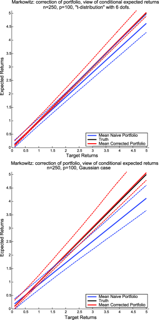
Figure 2: Performance of naive and corrected portfolios, for scaled “$t_{6}$” (top picture) and Gaussian returns. Here $n=250,p=100$ and the number of simulations is 1000. The dashed lines represent 95% confidence bands. The $x$-axis represents the returns an investor expects. The $y$-axis represents what she would actually get on average (i.e., $\mu^{\prime}\widehat{w}$). The plots show both the bias in the naive solution (blue solid lines) and the fact that our estimator is nearly unbiased (red solid lines). They also illustrate the robustness of our corrections. The black line is very close to the red line, showing a very good correction (on average) in this setting where assumptions A1–A5 are satisfied.

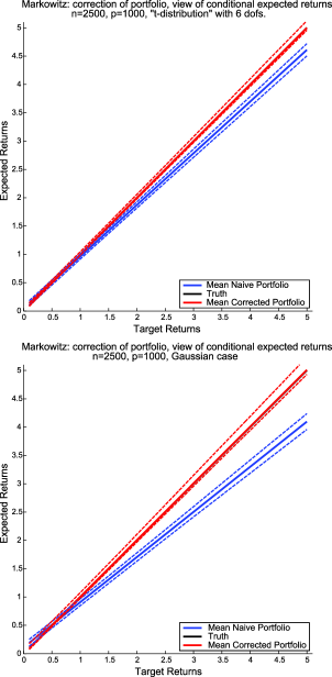
Figure 3: Performance of naive and corrected portfolios, for scaled “$t_{6}$” (left picture) and Gaussian returns. Here $n=2500,p=1000$ and the number of simulations is 1000. The dashed lines represent 95% confidence bands. The $x$-axis represents the returns an investor expects. The $y$-axis represents what she would actually get on average (i.e., $\mu^{\prime}\widehat{w}$). The plots show both the bias in the naive solution (blue solid lines) and the fact that our estimator is nearly unbiased (red solid lines). They also illustrate the robustness of our corrections. Note the narrower confidence bands as compared to Figure 2. The black line is essentially hidden under the red line, showing a near perfect correction (on average) in this setting where assumptions A1–A5 are satisfied.

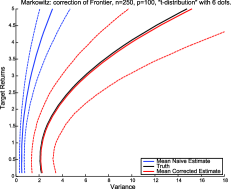
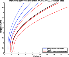
(a)	(b)
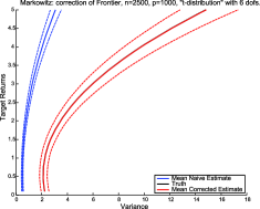
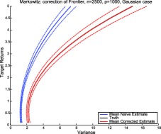
(c)	(d)

Figure 4: Performance of naive and corrected frontiers, for scaled “$t_{6}$” [(a) and (c)] and Gaussian returns [(b) and (d)]. Here, in the left column $n=250$ and $p=100$. In the right column, $n=2500,p=1000$. The number of simulations is 1000 in all pictures. The dashed lines represent (empirical) 95% confidence bands. (The confidence bands corresponds are computed for a fixed $y$.) The $x$-axis represents our estimate of variance of the optimal portfolio. The $y$-axis represents the target returns for the portfolio. The plots show both the bias in the naive solution (blue solid curves) and the fact that our estimator is nearly unbiased (red solid curves near, or covering the black curve, the population solution). They also illustrate the robustness of our corrections. Another striking feature is the lack of robustness of Gaussian computations, since the “efficient frontiers” computed with “$t_{6}$” returns are different from the Gaussian ones. The fact that, as our theoretical work predicts, Gaussian computations underestimate risk-underestimation in the class of elliptical distributions considered in the paper is illustrated by the fact that the “$t_{6}$” curves are to the left of the Gaussian curves. Note the narrower confidence bands in the larger dimensional simulations [(c) and (d)]. The black line is essentially hidden under the red line in (c) and (d), showing a near perfect correction (on average) in this setting where assumptions A1–A5 are satisfied.

5.5.1 Estimation of portfolio weights

As we have seen earlier, the “naive” weights obtained by plugging-in the sample mean and the sample covariance matrix in our quadratic program with linear equality constraints are biased, in the sense that their projection in any given direction will generally be biased.

Here we show the performance of our estimator as measured by its projection on $v_{k}=\mu$. It is a natural direction to consider since, for instance, in a financial context and under our modeling assumptions, it gives us the expected returns of our portfolio (conditional on $X_{1},\ldots,X_{n}$).

As our limited simulations indicate, our estimator appears to be practically unbiased here (even in the “lower-dimensional” case), which means in a financial context that the corresponding investment strategy will yield the returns that the investor expected. (We note that from a mean–variance point of view, we do not claim that our estimator is optimal. Work is under way to find better performing portfolios—but it requires a new set of theoretical investigations whose results are postponed to another paper. In limited simulations, it appeared that our “debiased” portfolio performed similarly to the naive one from a mean–variance point of view, its main advantage being that it delivers the returns that the investor expects.)

We present two pictures, Figure 2, page 2 and Figure 3, page 3 to give a sense to the reader of the impact of the size of $n$ and $p$ on the estimators we proposed [the “larger-dimensional” case gives quite significantly better results, with narrower confidence bands, though (empirical) near-unbiasedness is present in both cases].

5.5.2 Correction to the frontier

We now turn to the issue of estimating the “efficient frontier,” that is, the curve that represents the minima of our convex optimization problem (QP-eqc), on page QP-eqc. The pictures we present on Figure 3 (see page 4) were obtained from the simulations we described above. We chose to plot the variance (i.e., $\min w^{\prime}\Sigma w$) on the $x$-axis and the “target returns” [i.e., the $u_{k}$’s in the notation of equation (QP-eqc)] on the $y$-axis as this is the convention in financial applications.

As the reader can see, our estimator turns out to be essentially unbiased, even in the “lower-dimensional” case. We note too that the variance can be quite large but that the confidence bands obtained from our corrections were always to the right of the confidence bands obtained from the naive estimator, meaning that if one is concerned with risk estimation that in (essentially) the worst case for our estimator, we still obtained a better performing estimator than in (essentially) the best case for the naive estimator. (We do not claim that this is always the case and it might be an artifact of the simulation setup chosen here.)

Finally, for graphical purposes and to help comparisons, we chose to put all the graphs on the same scale. Some of the information on our original graphs (for the “lower-dimensional” case) was therefore left out but can be inferred by “naturally” extrapolating the curves shown on our graphs which are essentially parabolas.

5.6 Remarks on inequality constraints

Our work has mostly been concerned with obtaining results for the case of a quadratic program with linear equality constraints. We now explain that our results can also be used to obtain approximation results concerning the case of a quadratic program with linear inequality constraints.

In this subsection we therefore consider the problem

$$f_{\mathrm{theo}}(Q)=\cases{\displaystyle\inf_{w\in\mathbb{R}^{p}}w^{\prime}\Sigma w,\cr\displaystyle V^{\prime}w\in Q.}$$ (QP-ineqc-Pop)

Here $Q$ is a subset of $\mathbb{R}^{k}$, and $V$ is a $p\times k$ matrix. We naturally want to relate the solution of the above problem to that of the empirical version of the problem:

$$f_{\mathrm{emp}}(Q)=\cases{\displaystyle\inf_{w\in\mathbb{R}^{p}}w^{\prime}\hat{\Sigma}w,\cr\displaystyle\widehat{V}^{\prime}w\in Q.}$$ (QP-ineqc-Emp)

When $Q$ is a product of intervals, we obtain a quadratic program with linear inequality constraints. But our formulation allows us to deal with even more complicated constraint structures. We note that if $G(U)$ is the solution of problem (QP-ineqc-Pop) with $Q=\{U\}$ (i.e., a singleton), where $U$ is a vector in $\mathbb{R}^{k}$, we are back in the case of the equality constrained problem that we worked with for most of this paper. Let us call $\widehat{G}(U)$ the solution of problem (QP-ineqc-Emp) with $Q=\{U\}$. We now make the simple following observation: note that

$$f_{\mathrm{theo}}(Q) = \inf_{U\in Q}G(U),$$

$$f_{\mathrm{emp}}(Q) = \inf_{U\in Q}\widehat{G}(U).$$

The main idea here is that we can find a deterministic equivalent to $f_{\mathrm{emp}}(Q)$ and we can relate this deterministic equivalent to $f_{\mathrm{theo}}(Q)$.

Recall from Section 2 that $G(U)=U^{\prime}M^{-1}U$ and $\widehat{G}(U)=U^{\prime}\widehat{M}^{-1}U$. Recall also that under the assumptions A1–A5 made at the beginning of this section, we have found a deterministic equivalent to $\widehat{M}^{-1}$: we have shown that $\widehat{M}\simeq\mathfrak{s}M+\kappa_{n}e_{k}e_{k}^{\prime}=M_{0}(\mathfrak{s},\kappa_{n})$ in probability. The previous result is valid entry-wise, and since we assume that $k$ stays bounded in the asymptotics we are considering, it is also valid in operator norm. Now, $\widehat{M}$ is invertible with probability one under our assumptions, so we have, using the first resolvent identity, that is, $A^{-1}-B^{-1}=A^{-1}(B-A)B^{-1}$,

$$|\!|\!|\widehat{M}^{-1}-M^{-1}_{0}(\mathfrak{s},\kappa)|\!|\!|_{2}\leq|\!|\!|\widehat{M}^{-1}|\!|\!|_{2}|\!|\!|M_{0}^{-1}(\mathfrak{s},\kappa_{n})|\!|\!|_{2}|\!|\!|\widehat{M}-M_{0}(\mathfrak{s},\kappa_{n})|\!|\!|_{2}.$$

Hence, since $|\!|\!|M^{-1}|\!|\!|_{2}$ remains bounded under our assumptions,

$$|\!|\!|\widehat{M}^{-1}-M^{-1}_{0}(\mathfrak{s},\kappa)|\!|\!|_{2}\rightarrow 0\qquad\mbox{in probability}.$$

Under our assumptions, we also know that the smallest eigenvalue of $\widehat{M}$ and $M_{0}(\mathfrak{s},\kappa)$ stay bounded away from 0. Therefore, for any $\delta>0$, we know that asymptotically, and with probability 1,

$$\forall U\in\mathbb{R}^{k}\qquad|U^{\prime}\widehat{M}^{-1}U-U^{\prime}M^{-1}_{0}(\mathfrak{s},\kappa_{n})U|\leq\delta\|U\|_{2}^{2}.$$

Furthermore, let us note that assumption A2 guarantees that $|\!|\!|M|\!|\!|_{2}$ remains bounded and hence so do $|\!|\!|\widehat{M}|\!|\!|_{2}$ and $|\!|\!|M_{0}(\mathfrak{s},\kappa_{n})|\!|\!|_{2}$.

We have the following theorem.

Theorem 5.5

Suppose $G_{0}$ and $\widehat{G}_{n}$ are maps from $\mathbb{R}^{k}$ to $\mathbb{R}^{+}$ such that:

1. [3.]

2. $G_{0}$ is deterministic and $\widehat{G}_{n}$ is possibly random.

3. $G_{0}(0)=\widehat{G}_{n}(0)=0$.

4. $\exists c_{0}>0$ such that, $\forall U$, $G_{0}(U)\geq c_{0}\|U\|_{2}^{2}$. Similarly, $\exists\hat{c}_{n}>0$ such that, $\forall U$, $\widehat{G}_{n}(U)\geq\hat{c}_{n}\|U\|_{2}^{2}$. Furthermore, $\hat{c}_{n}\rightarrow c_{0}$ with probability 1.

5. $\exists\delta_{n}$ such that $\delta_{n}\rightarrow 0$ in probability and $\forall U$, $|\widehat{G}_{n}(U)-G_{0}(U)|\leq\delta_{n}\|U\|^{2}_{2}$.

Assume that $k$ is fixed as $n\rightarrow\infty$. Suppose $Q$ is a (nonempty) subset of $\mathbb{R}^{k}$ and that we can find $U_{0}\in Q$ such that $G_{0}(U_{0})<\infty$ and $U_{0}\neq 0$. Then,

$$\lim_{n\rightarrow\infty}\inf_{U\in Q}\widehat{G}_{n}(U)=\inf_{U\in Q}G_{0}(U)\qquad\mbox{in probability.}$$

We have the following corollary:

Corollary 5.6.

When assumptions A1–A5 are satisfied

$$f_{\mathrm{emp}}(Q)\rightarrow\inf_{U\in Q}U^{\prime}M^{-1}_{0}(\mathfrak{s},\kappa_{n})U\qquad\mbox{in probability}.$$

Hence, we have found a deterministic equivalent to $f_{\mathrm{emp}}(Q)$. It should also be noted that because $U^{\prime}M^{-1}_{0}(\mathfrak{s},\kappa_{n})U\leq\frac{1}{\mathfrak{s}}M^{-1}$, we also have

$$f_{\mathrm{emp}}(Q)\leq\frac{1}{\mathfrak{s}}\inf_{U\in Q}U^{\prime}M^{-1}U=\frac{1}{\mathfrak{s}}f_{\mathrm{theo}}(Q)\qquad\mbox{with high probability}.$$

Hence, our results on risk underestimation remain valid, even with these more general (nonequality) linear constraints. The comparison theorems between Gaussian and elliptical assumptions remain also valid, because of similar comparison theorems for their deterministic equivalents. [Note also that when $\widehat{M}\simeq\mathfrak{s}M$ (i.e., when the sample mean does not appear in $\widehat{V}$), the previous inequalities become equalities.] Finally, our corrections also give a way to get a consistent estimator of $f_{\mathrm{theo}}(Q)$: one can simply solve the optimization problem over $Q$ with $\widehat{M}$ replaced by $1/\widehat{\mathfrak{s}}(\widehat{M}-\kappa_{n}e_{k}e_{k}^{\prime})$ in the definition of $\widehat{G}$.

Note that the corollary follows immediately from Theorem 5.5 because of our remarks on the operator norm of $\widehat{M}$ and $\widehat{M}^{-1}$ and their deterministic equivalents.

Let us now prove Theorem 5.5. Proof of Theorem 5.5 Let us pick $U_{0}$ in $Q$. We can do so because $Q$ is nonempty. We assume without loss of generality that $0\notin Q$, for otherwise the problem is trivial, since $0$ is the global minimizer of both (deterministic and stochastic) problems.

Let us pick $r_{0}=\sqrt{2G_{0}(U_{0})/c_{0}}$, with $U_{0}\neq 0$. Suppose that $U\notin B(0,r_{0})$, where $B(0,r_{0})$ is the closed ball of radius $r_{0}$ with center $0$. Then, our assumptions on $G_{0}$ guarantee that

$$G_{0}(U)\geq c_{0}\|U\|_{2}^{2}>c_{0}\frac{2G_{0}(U_{0})}{c_{0}}=2G_{0}(U_{0}).$$

So $U_{0}\in B(0,r_{0})$. Also, if we call $Q(r_{0})=Q\cap B(0,r_{0})$, $Q(r_{0})$ is nonempty and

$$\inf_{U\in Q}G_{0}(U)=\inf_{U\in Q(r_{0})}G_{0}(U),$$

because if $U$ is outside of $B(0,r_{0})$, $G_{0}(U)>G_{0}(U_{0})$. Now, suppose that $\{\alpha_{t}\}_{t\in T}$ and $\{\beta_{t}\}_{t\in T}$ are two sets of real numbers. We have

$$|\inf\alpha_{j}-\inf\beta_{k}|\leq\sup|\alpha_{i}-\beta_{i}|.$$

As a matter of fact, for any $j$,

$$(\inf\alpha_{k})-\beta_{j}\leq\alpha_{j}-\beta_{j}\leq|\alpha_{j}-\beta_{j}|\leq\sup_{k}|\alpha_{k}-\beta_{k}|.$$

Now $\sup_{j}[(\inf\alpha_{k})-\beta_{j}]=(\inf\alpha_{k})-(\inf\beta_{k})$. And the previous display guarantees that $\sup_{j}[(\inf\alpha_{k})-\beta_{j}]\leq\sup_{k}|\alpha_{k}-\beta_{k}|$. By symmetry of the role of $\alpha$ and $\beta$, we therefore have

$$|\inf\alpha_{j}-\inf\beta_{k}|\leq\sup|\alpha_{i}-\beta_{i}|.$$

Hence, we can conclude that

$$\Bigl{|}\inf_{U\in Q(r_{0})}G_{0}(U)-\inf_{U\in Q(r_{0})}\widehat{G}_{n}(U)\Bigr{|}\leq\sup_{U\in Q(r_{0})}|G_{0}(U)-\widehat{G}_{n}(U)|\leq\delta_{n}r_{0}^{2},$$

by our assumptions, and the fact that $\|U\|_{2}^{2}\leq r_{0}^{2}$ in $Q(r_{0})$. Hence, since $r_{0}$ stays fixed as $n\rightarrow\infty$,

$$\Bigl{|}\inf_{U\in Q}G_{0}(U)-\inf_{U\in Q(r_{0})}\widehat{G}_{n}(U)\Bigr{|}\rightarrow 0\qquad\mbox{in probability.}$$

If we can show that with high-probability,

$$\inf_{U\in Q(r_{0})}\widehat{G}_{n}(U)=\inf_{U\in Q}\widehat{G}_{n}(U),$$

the result will be shown. First we note that if $U\notin B(0,r_{0})$,

$$\widehat{G}_{n}(U)\geq\hat{c}_{n}\frac{2G_{0}(U_{0})}{c_{0}}>(1+\delta)\widehat{G}_{n}(U_{0})$$

for some $\delta>0$ with high probability under our assumptions. Let us call $E_{\delta}$ the event $E_{\delta}=\{2\hat{c}_{n}/c_{0}>(1+\delta)\widehat{G}_{n}(U_{0})/G_{0}(U_{0})\}$. Of course, $P(E_{\delta})\rightarrow 1$ under our assumptions, since $2\hat{c}_{n}/c_{0}\rightarrow 2$ in probability and $\widehat{G}_{n}(U_{0})/G_{0}(U_{0})\rightarrow 1$ in probability. When $E_{\delta}$ is true, we have

$$\inf_{U\in B^{c}(0,r_{0})\cap Q}\widehat{G}_{n}(U)\geq(1+\delta)\widehat{G}_{n}(U_{0})>\widehat{G}_{n}(U_{0})\geq\inf_{U\in Q(r_{0})}\widehat{G}_{n}(U).$$

So when $E_{\delta}$ is true, and hence with high-probability,

$$\inf_{U\in Q}\widehat{G}_{n}(U)=\inf_{U\in Q(r_{0})}\widehat{G}_{n}(U).$$

We can finally conclude that

$$\inf_{U\in Q}\widehat{G}_{n}(U)\rightarrow\inf_{U\in Q}G_{0}(U)\qquad\mbox{in probability,}$$

and the theorem is proved.

6 Conclusion

This study of quadratic programs with linear constraints whose parameters are estimated from data has highlighted the difficulties created by the high-dimensionality of the data. In particular, we have shown that the fact that $n$ (the number of observations used to estimate the parameters) and $p$ both grew to infinity lead to a systematic underestimation of the minimal “risk” one exposed oneself to when approaching the optimization problem (QP-eqc-Pop) by solving its naive proxy (QP-eqc-Emp).

Our study produced exact distributional results in the Gaussian case (Section 3) and convergence results in probability in the elliptical case (Section 4), which also allowed us to reach conclusions for the bootstrap and the case of nonindependent data (in particular, it covers the case of Gaussian data correlated in time). As explained in Section 5, the study of the Gaussian case gives an over-optimistic assessment of risk underestimation in the context we study: in the class of elliptical distributions we consider, risk is minimally underestimated in the Gaussian case, and the situation is more dire for other elliptical distributions. Our study also highlights the fact that standard bootstrap estimates of bias will be inconsistent. It also suggests that in the case of correlated Gaussian observations, risk underestimation is likely to be more severe than in the i.i.d. case.

Another benefit of our analysis is that it sheds light on what is creating those difficulties and allows us to propose robust corrections to these problems. As shown in the theoretical part of the paper and illustrated in our limited simulation work, they are robust in the class of elliptical distributions we consider. They also appear to work reasonably well in practice (when the underlying assumptions hold), as our (somewhat limited) simulation work seems to indicate.

Perhaps surprisingly, we did not need to make very strong assumptions about the covariance matrix at stake or the mean, whereas recent statistical work focused on estimation of covariance matrices [see El Karoui (2008) or Bickel and Levina (2008b)] tends to do so. This is in part because our theoretical analysis clearly showed what functionals of these two parameters one needed to estimate, and hence we were able to bypass stronger requirements by focusing on those particular functionals and correcting the first order errors that appeared. In other words, even though our aim was to estimate a complicated function of the population covariance matrix and of the population mean, for which we do not have good estimators in high-dimension in general, we were able to use poor estimators of both (and our theoretical analysis) to get an accurate estimator of the functional of interest. This is an interesting result in the context of high-dimensional statistics more generally, as it suggests that we might be able to estimate certain functions of high-dimensional parameters without having to accurately estimate the parameters themselves [and hence we might be able to bypass in some situations sparsity (or other similar requirements) for the population quantities].

Beside the interesting statistical and mathematical questions this study raised, we hope that it might also be helpful to, for instance, financial regulators by perhaps providing them with more realistic benchmarks for the performance of optimal portfolios and that it sheds light on how the high-dimensionality of the data affects the proper assessment of risk of large portfolios obtained by solving high-dimensional optimization problems.

Appendix A Classical results of linear algebra

A.1 On inverses of partitioned matrices

In our study of the Gaussian case, and in particular in connection with properties of Wishart matrices, we relied several times on properties of the inverse of a partitioned matrix. Here is a detailed statement of what we needed.

Let $A$ be a generic matrix, and let us decompose it by blocks

$$A=\pmatrix{A_{11}&A_{12}\cr A_{21}&A_{22}}.$$

Let us call $A^{-1}$ the inverse of $A$. We assume that all inverses we take are well defined. Let us write

$$A^{-1}=\pmatrix{A^{11}&A^{12}\cr A^{21}&A^{22}}.$$

Then, it is well known that [see, e.g., Mardia, Kent and Bibby (1979), pages 458–459, or Boyd and Vandenberghe (2004), page 650]

$$A^{11} = (A_{11}-A_{12}A_{22}^{-1}A_{21})^{-1},$$ (A.1)

$$A^{22} = (A_{22}-A_{21}A_{11}^{-1}A_{12})^{-1},$$ (A.2)

$$A^{12} = -A_{11}^{-1}A_{12}A^{22},$$ (A.3)

$$A^{21} = -A^{22}A_{21}A_{11}^{-1}.$$ (A.4)

Appendix B Random matrix results

B.1 Lower bounds on smallest eigenvalue

In many proofs in the course of the paper we needed to have quantitative bounds on the behavior of the smallest eigenvalue of a number of matrices and made repeated use of the following lemma.

Lemma B.1

Suppose $Y$ is a $n\times p$ matrix, with i.i.d. ${\cal N}(0,1)$ entries, with $p/n\rightarrow\rho$, and $0<\rho<1$.

Suppose $\Lambda$ is an $n\times n$ diagonal and deterministic matrix and that we can find $N$, $C>0$ and $\varepsilon>0$ such that, if $\tau_{i}$ is the $i$th largest eigenvalue of $\Lambda^{\prime}\Lambda$, $\tau_{N}>C$, for some fixed $C>0$. $N$ is such that, for $p$ and $n$ large, $p/N<1-\varepsilon$ and $N/n$ stays bounded away from 0. Finally, we assume that all the diagonal entries of $\Lambda$ are different from 0.

Call $H=\mathrm{Id}-\delta\delta^{\prime}/n$, where $\|\delta\|_{2}^{2}=n$. Then $\lambda_{p}$, the smallest eigenvalue of $Y^{\prime}\Lambda^{\prime}H\Lambda Y/n-1$, is bounded away from 0 with high-probability.

In particular, when $p/N<1-\varepsilon$, if $\mathfrak{C}_{n}=C\frac{N-1}{n-1}$,

$$P\bigl{(}\sqrt{\lambda_{p}}\leq\sqrt{\mathfrak{C}_{n}}\bigl{[}\bigl{(}1-\sqrt{1-\varepsilon}\bigr{)}-t\bigr{]}\bigr{)}\leq\exp\bigl{(}-(N-1)t^{2}\bigr{)}.$$

The following proof makes clear that the result holds also when some of the diagonal entries of $\Lambda$ are equal to zero if we make the following modification: $n$ should now denote the number of nonzero entries on the diagonal of $\Lambda$, and the corresponding assumptions about $p$ and $N$ should then hold. We also point out that under our assumptions $H$ is an orthogonal projection matrix.

Proof of Lemma B.1 Before we start the proof per se, we need some notations: we call $\lambda_{k}$ the $k$th largest eigenvalue of a symmetric matrix. In other words, the eigenvalues are decreasingly ordered and $\lambda_{1}\geq\lambda_{2}\geq\cdots.$

The result is known if $\Lambda=\mathrm{Id}_{n}$, since

$$\frac{1}{n-1}Y^{\prime}HY\stackrel{{\scriptstyle{\cal L}}}{{=}}\frac{1}{n-1}\cal{W}_{p}(\mathrm{Id}_{p},n-1).$$

Using Davidson and Szarek (2001), Theorem II.13, we have the following result: the smallest eigenvalue of a matrix with distribution $\cal{W}(\mathrm{Id}_{p},n_{0})/n_{0}$ is strongly concentrated around $(1-\sqrt{p/n_{0}})^{2}$ when $p<n_{0}$, and

$$P\bigl{(}\sqrt{\lambda_{p}}<\bigl{(}1-\sqrt{p/n_{0}}\bigr{)}-t\bigr{)}\leq\exp(-n_{0}t^{2}).$$

This gives our result in the case where $\Lambda=\mathrm{Id}_{n}$. Let us now investigate what happens when $\Lambda$ is not $\mathrm{Id}_{n}$.

The matrix $M=\Lambda^{\prime}H\Lambda$ is a rank-1 perturbation of $\Lambda^{\prime}\Lambda$ and is positive semi-definite, because $H$ is. Therefore, for any $k\geq 2$, $\lambda_{k-1}(\Lambda^{\prime}H\Lambda)=\lambda_{k-1}(M)\geq\lambda_{k}(\Lambda^{\prime}\Lambda)$, by the interlacing Theorem 4.3.4 in Horn and Johnson (1990). $M$ has rank $n-1$ matrix since, $M\Lambda^{-1}\delta=0$ and $\textrm{rank}(M)\geq\textrm{rank}(\Lambda^{\prime}\Lambda)-1=n-1$.

We can diagonalize $M=ODO^{\prime}$, where $D$ has $(n-1)$ nonzero coefficients, and because $O^{\prime}Y\stackrel{{\scriptstyle{\cal L}}}{{=}}Y$, we have

$$Y^{\prime}MY=Y^{\prime}\Lambda^{\prime}H\Lambda Y\stackrel{{\scriptstyle{\cal L}}}{{=}}Y^{\prime}DY=\sum_{i=1}^{n-1}d_{i}Y_{i}Y_{i}^{\prime},$$

where $d_{i}$ are the nonzero diagonal entries of $D$. Because $M$ is positive semi-definite, we have $d_{i}\geq 0$ for all $i$. In other respects, because for all $k\leq n-1$, $d_{k}\geq\lambda_{k+1}(\Lambda^{\prime}\Lambda)=\tau_{k+1}$ by our remark on interlacing inequalities. Hence, we have, if $\succeq$ denotes positive-semidefinite ordering,

$$\sum_{i=1}^{n-1}d_{i}Y_{i}Y_{i}^{\prime}\succeq\sum_{i=1}^{N-1}d_{i}Y_{i}Y_{i}^{\prime}\succeq\tau_{N}\sum_{i=1}^{N-1}Y_{i}Y_{i}^{\prime}=\tau_{N}\cal{W}_{p}(\mathrm{Id}_{p},N-1).$$

Therefore, we have in law,

$$\frac{1}{n-1}Y^{\prime}\Lambda^{\prime}H\Lambda Y\succeq C\frac{N-1}{n-1}\frac{1}{N-1}\cal{W}_{p}(\mathrm{Id}_{p},N-1).$$

As we recalled above, the smallest eigenvalue of $\cal{W}_{p}(\mathrm{Id}_{p},N-1)/(N-1)$ remains bounded away from 0 with high-probability in our setting because $p/N$ remains bounded away from 1 by assumption. We also assumed that $N/n$ and $C$ were bounded away from 0. If we call $\mathfrak{C}=\liminf_{n\rightarrow\infty}C\frac{N-1}{n-1}$, we have $\mathfrak{C}>0$, and, for any $\eta>0$, according to the result of Davidson and Szarek (2001) we have, for $\lambda_{p}=\lambda_{p}(\frac{1}{n-1}Y^{\prime}\Lambda^{\prime}H\Lambda Y)$ and $\mathfrak{C}_{n}=C(N-1)/(n-1)$,

$$P\bigl{(}\sqrt{\lambda_{p}}\leq\sqrt{\mathfrak{C}_{n}}\bigl{[}\bigl{(}1-\sqrt{p/(N-1)}\bigr{)}-t\bigr{]}\bigr{)}\leq\exp\bigl{(}-(N-1)t^{2}\bigr{)}.$$

In particular, when $p/N$ is such that $p/N\leq 1-\varepsilon$,

$$P\bigl{(}\sqrt{\lambda_{p}}\leq\sqrt{\mathfrak{C}_{n}}\bigl{[}\bigl{(}1-\sqrt{1-\varepsilon}\bigr{)}-t\bigr{]}\bigr{)}\leq\exp\bigl{(}-(N-1)t^{2}\bigr{)}.$$

Interestingly, this bound is “quite uniform” in $\Lambda$, in the sense that the only characteristics of $\Lambda$ that matter are $\mathfrak{C}_{n}=C\frac{N-1}{n-1}$ and $N$.

Appendix C Generalizations of the proof of Theorem 4.3

This part of the Appendix explains how to appropriately modify the proofs of Theorems 4.1 and  4.6 to obtain the results we need in the case of correlated observations (Section 4.3) and the bootstrap.

C.1 On ${v^{\prime}\hat{\Sigma}^{-1}v}$ when the observations are correlated

We explain in this subsection how to modify the proof of Theorem 4.1 in the case where the vectors of observations $X_{i}$ and $X_{j}$ are potentially correlated. The data was assumed to have the following representation, in matrix form:

$$X=\mathbf{e}\mu^{\prime}+\Lambda Y\Sigma^{1/2},$$

where $\Lambda$ is $n\times n$, deterministic but not necessarily diagonal and $Y$ has i.i.d. ${\cal N}(0,1)$ entries. We also wrote the SVD of $\Lambda$ as $\Lambda=ADB^{\prime}$, where $A$ and $B$ are orthogonal.

If we call $H=\mathrm{Id}_{n}-\mathbf{e}\mathbf{e}^{\prime}/n$, we have, of course,

$$\hat{\Sigma}=\frac{1}{n-1}X^{\prime}HX=\frac{1}{n-1}\Sigma^{1/2}Y^{\prime}\Lambda^{\prime}H\Lambda Y\Sigma^{1/2}.$$

The orthogonality of $B$ implies $BY\stackrel{{\scriptstyle{\cal L}}}{{=}}Y$, and we have

$$\hat{\Sigma}\stackrel{{\scriptstyle{\cal L}}}{{=}}\frac{1}{n-1}\Sigma^{1/2}Y^{\prime}D(A^{\prime}HA)DY\Sigma^{1/2}.$$

If we now call $\delta=A^{\prime}\mathbf{e}$, we see that $\|\delta\|_{2}^{2}=n$, because $A$ is orthogonal. It can also easily be seen that $A^{\prime}HA=\mathrm{Id}_{n}-\delta\delta^{\prime}/n=H_{\delta}$. Because of the remark we just made on the norm of $\delta$, $H_{\delta}$ is clearly an orthogonal projection matrix. So we have to understand

$$\hat{\Sigma}\stackrel{{\scriptstyle{\cal L}}}{{=}}\frac{1}{n-1}\Sigma^{1/2}Y^{\prime}DH_{\delta}DY\Sigma^{1/2},$$

which is extremely close to the situation of Theorem 4.1, where we had to work with

$$\hat{\Sigma}\stackrel{{\scriptstyle{\cal L}}}{{=}}\frac{1}{n-1}\Sigma^{1/2}Y^{\prime}DH_{\mathbf{e}}DY\Sigma^{1/2}.$$

$D$ now plays the role $\Lambda$ played in Theorem 4.1 and the main modification is that $H=H_{\mathbf{e}}$ is now replaced by $H_{\delta}$.

An examination of the proof of Theorem 4.1 shows that we never relied on the fact that we used specifically $H_{\mathbf{e}}$ (instead of $H_{\delta}$) in that proof. All we used was the fact that our $H$ there was a rank-1 perturbation of $\mathrm{Id}_{n}$ and an orthogonal projection matrix. Similarly, Lemma B.1, on which we relied in the course of the proof of Theorem 4.1, handles $H_{\delta}$ for general $\delta$ with squared norm $n$ without any problems, so it is still usable in the course of the current study.

Because we know that the squared singular values of $\Lambda$ (and hence the eigenvalues of $D$) satisfy (Assumption-BB), the proof of Theorem 4.1 goes through without further modifications and Proposition 4.7 holds.

C.2 On quadratic forms involving random projection matrices

A recurrent issue in the questions we addressed was the understanding of statistics of the form

$$\frac{1}{n}u^{\prime}Pu,$$

where $P$ is a random projection matrix and $u$ a (generally deterministic) vector of dimension $n$. In particular, the projection matrices we dealt with were of the form

$$P=\Lambda Y(Y^{\prime}\Lambda^{2}Y)^{-1}Y^{\prime}\Lambda,$$

for $\Lambda$ a (possibly random) $n\times n$ diagonal matrix and $Y$ an $n\times p$ matrix with i.i.d. ${\cal N}(0,1)$ entries. We also assume that $\Lambda$ and $u$ are independent of $Y$. Finally, we assume that $\|u\|_{2}/\sqrt{n}=1$.

In the course of the text, we carried out successfully computations when $u=\mathbf{e}$, but relied to do so on properties of $\operatorname{trace}(P)$. The case of general $u$ is more involved and is treated here.

Lemma C.1

Assume that $\Lambda$ and u (which is deterministic) are such that

$$\frac{1}{n^{2}}\sum_{i=1}^{n}u_{i}^{4}\rightarrow 0\quad\mbox{and}\quad\frac{1}{n^{2}}\sum_{i=1}^{n}\lambda_{i}^{4}\rightarrow 0$$

and that (Assumption-BB) holds for $\Lambda$ for a certain sequence $N(n)$.

Under the preceding assumptions, we have, if $Z(u)=\frac{1}{n}u^{\prime}Pu$,

$$Z(u)-\frac{1}{n}\sum_{i=1}^{n}u_{i}^{2}\mathbf{E}(P(i,i)|\Lambda)\rightarrow 0\qquad\mbox{in probability}$$

conditionally on $\Lambda$.

We simply sketch the modifications to the proof given after the statement of Theorem 4.3. As noted in Lemma 4.4, the off-diagonal elements of $P$ have mean 0 conditionally on $\Lambda$. Now, using the same notations as in Theorem 4.3, we have, using equation (4.2) there, if $Z_{i}(u)$ is the quantity obtained by replacing $\lambda_{i}$ by $0$ in $Z$, $r_{i}=W_{i}{\cal S}_{i}^{-1}Y_{i}$, $w_{i}=r_{i}^{\prime}u/n$ and $u_{i}$ is the $i$th coordinate of $u$,

$$Z(u)=Z_{i}(u)+\frac{1}{n}\frac{1}{1+\lambda_{i}^{2}q_{i}}(-\lambda_{i}^{2}w_{i}^{2}+2\lambda_{i}u_{i}w_{i}+\lambda_{i}^{2}u_{i}w_{i}).$$

The expression between the parentheses is easily seen to be equal to $(1+\lambda_{i}^{2}q_{i})u_{i}^{2}-(\lambda_{i}w_{i}-u_{i})^{2}$. We get an analog of equation (8)

$$Z(u)=Z_{i}(u)+\frac{u_{i}^{2}}{n}-\frac{1}{n}\frac{(\lambda_{i}w_{i}-u_{i})^{2}}{1+\lambda_{i}^{2}q_{i}}.$$

Clearly, from the definition of $w_{i}$, $w_{i}|\{Y_{(-i)},\Lambda\}\sim{\cal N}(0,u^{\prime}W_{i}{\cal S}_{i}^{-2}W_{i}^{\prime}u/n^{2}).$ Since by assumption $\|u\|_{2}=\sqrt{n}$, we have

$$0\leq u^{\prime}W_{i}{\cal S}_{i}^{-1}W_{i}^{\prime}u/n^{2}=u^{\prime}W_{i}(W_{i}^{\prime}W_{i})^{-1}W_{i}^{\prime}u/n\leq 1$$

because $W_{i}(W_{i}^{\prime}W_{i})^{-1}W_{i}^{\prime}$ is an orthogonal projection matrix (hence its eigenvalues are only 0 and 1) and $\|u/\sqrt{n}\|_{2}=1$.

So we are exactly in the situation we were in during the proof of Theorem 4.3, except for a term in $u_{i}^{4}$ that now appears in our bound on the variance. Hence, with our extra assumption on $\|u\|_{4}^{4}/n^{2}$, we conclude similarly (after a regularization step) that $Z(u)$ converges in probability, conditional on $\Lambda$ to its conditional mean which is simply

$$\frac{1}{n}u_{i}^{2}\mathbf{E}(P(i,i)|\Lambda).$$

We remark that to get an analog of Theorem 4.5, where now

$$\zeta=\frac{1}{n}u^{\prime}\Lambda Y{\cal S}^{-1}v,$$

one just needs to go through the proof and replace the $w_{i}$ appearing there by the “new” $w_{i}=u^{\prime}W_{i}{\cal S}_{i}^{-1}Y_{i}/n$. Exactly the same arguments go through when $\sum_{i=1}^{n}u_{i}^{2}\lambda_{i}^{2}/n$ remains bounded. So under this condition, $\zeta$ tends to zero in probability.

With the help of the previous lemma, we can now prove the gist of Proposition 4.8.

Fact C.1

Proposition 4.8 holds.

We note that Proposition 4.8 is essentially an application of the previous lemma, with appropriate change of notation. Recall the notations from the proposition. We have $\widetilde{X}=\Lambda Y\Sigma^{1/2}$ and $\Lambda$, which is $n\times n$, has singular value decomposition $ADB^{\prime}$. Also, ${\cal S}=\widetilde{X}^{\prime}\widetilde{X}/n$, $\widetilde{Y}=B^{\prime}Y$, $F=\widetilde{Y}^{\prime}D^{2}\widetilde{Y}/n$. Hence, in the language of the proposition,

$$\hat{m}^{\prime}{\cal S}^{-1}\hat{m}=\frac{1}{n^{2}}\mathbf{e}^{\prime}AD\widetilde{Y}F^{-1}\widetilde{Y}^{\prime}DA\mathbf{e}=\omega^{\prime}P\omega,$$

where $P=D\widetilde{Y}(\widetilde{Y}^{\prime}D^{2}\widetilde{Y})^{-1}\widetilde{Y}^{\prime}D$ and $\omega=A^{\prime}\mathbf{e}$. When the assumptions of the proposition are in force, $\Lambda$ is deterministic and Lemma C.1 applies; from which we conclude

$$\hat{m}^{\prime}{\cal S}^{-1}\hat{m}-\frac{1}{n}\sum_{i=1}^{n}\omega_{i}^{2}\mathbf{E}(P(i,i))\rightarrow 0\qquad\mbox{in probability}.$$

This gives us the analog of Theorem 4.3.

To get the analog of Theorem 4.5, we just need $\sum_{i=1}^{n}\omega_{i}^{2}d_{i}^{2}/n$ to remain bounded, which is an assumption stated in Proposition 4.8.

C.3 Bootstrap specific results

Bootstrapping mean 0 Gaussian data

Our analysis of the bootstrap problem requires an analysis similar to the one we performed in the previous subsection. In particular, there we have $u=\Lambda^{1/2}\mathbf{e}$, where $\Lambda$ contains the bootstrap weights. Since those add-up to $n$, the assumption $\|u\|_{2}^{2}=n$ was clearly satisfied. Also, in the situation where $p/n\rightarrow\rho\in(0,1-1/e)$, we are guaranteed that

$$P^{*}=\Lambda^{1/2}Y(Y^{\prime}\Lambda Y)^{-1}Y^{\prime}\Lambda^{1/2}$$

is well defined with high-probability. When conditioning on $\Lambda$, we see that we can work only with the submatrix $\Lambda^{*}$ (of size $n^{*}$) whose diagonal entries are nonzero. This submatrix has its diagonal entries bounded away from 0 as they are at least equal to 1. Also, using arguments similar to those given in the proof of Lemma B.1, we see that we can get a uniform (in $\Lambda$) lower bound on the smallest singular value of $\Lambda Y$, which holds with probability exponentially [in $(n^{*}-p)$] close to 1.

So now we assume that we are dealing with $\Lambda$ such that $n^{*}-p$ tends to $\infty$, the empirical distribution of $\Lambda$ goes to $\mathrm{Po}(1)$ and $\sum\lambda_{i}^{2}/n^{2}\rightarrow 0$. We also assume that (Assumption-BB) are satisfied for this $\Lambda$. Finally, we assume that $\{\sum_{i=1}^{n}\lambda_{i}^{2}/n\leq 10\}$. We call the corresponding set of matrices ${\cal G}_{B_{n}}$. When the diagonal entries of $\Lambda$ are drawn from a multinomial$(\frac{1}{n},\ldots,\frac{1}{n},n)$ it is clear that these conditions are satisfied with probability going to 1. The only thing that might require an explanation is why the condition $\{\sum_{i=1}^{n}\lambda_{i}^{2}/n\leq 10\}$ holds with probability going to 1. The mean of $\sum_{i=1}^{n}\lambda_{i}^{2}/n$ clearly goes to 2, using the marginal distribution of $\lambda_{i}$. On the other hand, the arguments we gave in Proposition 4.10 show that its variance goes to 0, so this quantity goes to 2 in probability and therefore is less than 10 with probability going to 1.

The main question that we still have to address is that of the behavior of

$$\frac{1}{n}\sum_{i=1}^{n}u_{i}^{2}\mathbf{E}(P^{*}(i,i)|\Lambda)$$

when $u_{i}^{2}=\lambda_{i}$. By definition,

$$P^{*}(i,i)=\frac{1}{n}\lambda_{i}Y_{i}^{\prime}\Biggl{(}\frac{1}{n}\sum_{i=1}^{n}\lambda_{i}Y_{i}Y_{i}^{\prime}\Biggr{)}^{-1}Y_{i}=1-\frac{1}{1+\lambda_{i}Y_{i}^{\prime}{\cal S}_{i}^{-1}Y_{i}/n},$$

where ${\cal S}_{i}=\frac{1}{n}\sum_{j\neq i}\lambda_{j}Y_{j}Y_{j}^{\prime}$. Now concentration arguments (see, e.g., Section 5.6) show that, if $\sigma_{p}({\cal S}_{i})$ is the smallest singular value of ${\cal S}_{i}$,

$$P\biggl{(}\biggl{|}\frac{Y_{i}^{\prime}{\cal S}_{i}^{-1}Y_{i}}{p}-\frac{\operatorname{trace}({\cal S}_{i}^{-1})}{p}\biggr{|}>t\big{|}{\cal S}_{i}^{-1}\biggr{)}=\mathrm{O}\bigl{(}\exp\bigl{(}-pt^{2}\sigma^{2}_{p}({\cal S}_{i})/2\bigr{)}\bigr{)}.$$

We also know that with overwhelming probability (measured over $Y_{(-i)}=\{Y_{1},\ldots,Y_{i-1},Y_{i+1},\ldots,Y_{n}\}$), $\sigma_{p}({\cal S}_{i})$ is bounded away from 0, conditionally on $\Lambda$, when $\Lambda$ is such that (Assumption-BB) holds. (Note for instance that ${\cal S}_{i}\succeq\sum_{i\neq j}Y_{j}Y_{j}^{\prime}/n$ and use Lemma B.1.) Hence, we conclude that

$$\frac{Y_{i}^{\prime}{\cal S}_{i}^{-1}Y_{i}}{p}\simeq\frac{\mathrm{trace}({\cal S}_{i}^{-1})}{p}.$$

Hence, conditionally on $\Lambda$,

$$P^{*}(i,i)\simeq 1-\frac{1}{1+\lambda_{i}({p/n})({\mathrm{trace}({\cal S}_{i}^{-1})/p})},$$

with very high-probability, that is, the probability that the difference between the two is greater than $\lambda_{i}(p/n)t$ is $\mathrm{O}(\exp(-C(n^{*}-p)t^{2}))$ for a fixed $C$ (by arguments similar to those given in Lemma B.1). In other respects, we note that rank-1 perturbation arguments give, if ${\cal S}=\frac{1}{n}Y^{\prime}\Lambda Y$,

$$\operatorname{trace}({\cal S}_{i}^{-1})-\operatorname{trace}({\cal S}^{-1})=\frac{\lambda_{i}}{n}\frac{Y_{i}^{\prime}{\cal S}_{i}^{-2}Y_{i}}{1+\lambda_{i}Y_{i}^{\prime}{\cal S}_{i}^{-1}Y_{i}/n}.$$

In particular, when $\Lambda$ is such that (Assumption-BB) holds, by using a union bound argument,

$$P\biggl{(}\max_{i=1,\ldots,n}\biggl{|}\frac{\mathrm{trace}({\cal S}_{i}^{-1})-\operatorname{trace}({\cal S}^{-1})}{p}\biggr{|}>\varepsilon\big{|}\Lambda\biggr{)}\rightarrow 0.$$

We also note that $\operatorname{trace}({\cal S}^{-1})/p\rightarrow\mathfrak{s}$ conditionally on $\Lambda$, if $\Lambda$ is such that its empirical distribution goes to $\mathrm{Po}(1)$, $\Lambda\in{\cal G}_{B_{n}}$ and $p/n\rightarrow\rho$.

Therefore, we also have by a simple union bound argument, conditional on $\Lambda$, and assuming that $\Lambda$ is such that its empirical distribution goes to $\mathrm{Po}(1)$, $\Lambda\in{\cal G}_{B_{n}}$ and hence $\sum\lambda_{i}^{2}/n$ is less than 10,

$$\frac{1}{n}\sum_{i=1}^{n}\lambda_{i}P^{*}(i,i)\simeq 1-\frac{1}{n}\sum_{i=1}^{n}\frac{\lambda_{i}}{1+\lambda_{i}\rho_{n}\mathfrak{s}}.$$

Now when $\Lambda\Longrightarrow\mathrm{Po}(1)$, which we write $G$, and $\rho_{n}\rightarrow\rho$,

$$\frac{1}{n}\sum_{i=1}^{n}\frac{\lambda_{i}}{1+\lambda_{i}\rho_{n}\mathfrak{s}}\rightarrow\int\frac{\tau\,dG(\tau)}{1+\tau\rho\mathfrak{s}}.$$

But in light of the Marčenko–Pastur equation, we have, under these circumstances,

$$\frac{1}{n}\sum_{i=1}^{n}\lambda_{i}P^{*}(i,i)\rightarrow 1-\frac{1}{\mathfrak{s}}=\frac{\mathfrak{s}-1}{\mathfrak{s}}.$$

We finally conclude that conditional on $\Lambda$ being in ${\cal G}_{B_{n}}$ (whose probability goes to 1),

$$(\hat{\mu}^{*})^{\prime}(\hat{\Sigma}^{*})^{-1}\hat{\mu}^{*}\rightarrow\frac{(\mathfrak{s}-1)/\mathfrak{s}}{1-({\mathfrak{s}-1})/{\mathfrak{s}}}=\mathfrak{s}-1\geq\frac{\rho}{1-\rho},$$

since we know that $\mathfrak{s}\geq 1/(1-\rho)$ when $G$ is $\mathrm{Po}(1)$, since its mean is 1.

Similar arguments as the ones used in the proofs in the main body of the paper show that the same convergence in probability result holds unconditionally on $\Lambda$, the problem being to get bounds that are uniform in $\Lambda$, when $\Lambda\in{\cal G}_{B_{n}}$.

Hence, an analog of Theorem 4.3 follows (with ${\cal P}_{n}$ probability going to 1), where the ratio $\rho/(1-\rho)$ is replaced by $\mathfrak{s}-1$. The analog of Theorem 4.5 follows from the arguments given in Appendix C.2, if we can show, in the notation used there that $\sum_{i=1}^{n}(u_{i}d_{i})^{2}/n$ remains bounded with probability going to 1. Note that $u_{i}=d_{i}=\sqrt{\lambda_{i}}$ here, where $\lambda_{i}$ are the bootstrap weights, so we just need to show that $\sum_{i=1}^{n}\lambda_{i}^{2}/n$ remains bounded. But we did this when describing ${\cal G}_{B_{n}}$.

We therefore have an analog of Theorem 4.5 and also of Theorem 4.6 when bootstrapping Gaussian data.

Bootstrapping elliptically distributed data

Finally, let us say a few words about what would happen if we replaced the normality assumption for the $X_{i}$’s by an elliptical distribution assumption. We focus on the case where $X_{i}=\lambda_{i}\Sigma^{1/2}Y_{i}$, that is, the mean of the $X_{i}$’s is 0. The previous analyses make clear that the key questions concern $v^{\prime}(\hat{\Sigma}^{*})^{-1}v$ and $(\hat{\mu}^{*})^{\prime}(\hat{\Sigma}^{*})^{-1}\hat{\mu}^{*}$.

The questions concerning $v^{\prime}(\hat{\Sigma}^{*})^{-1}v$ fall pretty much directly under the study we have made of elliptical distributions, since we know, according to the proof of Theorem 4.12, that

$$\hat{\Sigma}^{*}=\frac{1}{n-1}\Sigma^{1/2}Y^{\prime}\Lambda^{\prime}D^{1/2}(\mathrm{Id}_{n}-\delta\delta^{\prime}/n)D^{1/2}\Lambda Y\Sigma^{1/2},$$

where $D$ is the diagonal matrix containing the bootstrap weights and $\delta=D^{1/2}\mathbf{e}$. So, as long as $D^{1/2}\Lambda$ satisfies (Assumption-BB), results similar to Theorem 4.12 will hold.

The questions dealing with $(\hat{\mu}^{*})^{\prime}(\hat{\Sigma}^{*})^{-1}\hat{\mu}^{*}$ are more involved. Analyses similar to the ones performed above show that the key quantity to understand is now

$$\frac{1}{n}\mathbf{e}^{\prime}D\Lambda Y(Y^{\prime}\Lambda^{\prime}D\Lambda Y)^{-1}Y^{\prime}\Lambda^{\prime}D\mathbf{e}=\frac{1}{n}u^{\prime}P_{D^{1/2}\Lambda,Y}u,$$

where $P_{D^{1/2}\Lambda,Y}=D^{1/2}\Lambda Y(Y^{\prime}\Lambda^{\prime}D\Lambda Y)^{-1}Y^{\prime}\Lambda D^{1/2}$ and $u=D^{1/2}\mathbf{e}$. The analysis of this quadratic form can be carried out just like we did above in the Gaussian case, that is, $\Lambda=\mathrm{Id}_{n}$. However, the remarks we made to get simplified expressions for the limit do not seem to apply anymore: quantities of the type

$$\frac{1}{n}\sum_{i=1}^{n}\frac{d_{i}}{1+\lambda_{i}^{2}d_{i}\rho\mathfrak{s}},$$

appear, where $\mathfrak{s}$ is the solution of equation (4) with $G$ being the limit (if it exists) of the empirical distribution of the random variables $\lambda_{i}^{2}d_{i}$. These quantities do not appear to simplify any further to yield a clearer and more exploitable expression.

References

- Anderson (2003) Anderson, T. W. (2003). An Introduction to Multivariate Statistical Analysis, 3rd ed. Wiley, Hoboken, NJ. \MR1990662
- Bai (1999) Bai, Z. D. (1999). Methodologies in spectral analysis of large-dimensional random matrices, a review. Statist. Sinica 9 611–677. With comments by G. J. Rodgers and Jack W. Silverstein; and a rejoinder by the author. \MR1711663
- Bai, Liu and Wong (2009) Bai, Z., Liu, H. and Wong, W.-K. (2009). Enhancement of the applicability of Markowitz’s portfolio optimization by utilizing random matrix theory. Math. Finance 19 639–667. \MR2583523
- Bickel and Levina (2008a) Bickel, P. J. and Levina, E. (2008a). Covariance regularization by thresholding. Ann. Statist. 36 2577–2604. \MR2485008
- Bickel and Levina (2008b) Bickel, P. J. and Levina, E. (2008b). Regularized estimation of large covariance matrices. Ann. Statist. 36 199–227. \MR2387969
- Biroli, Bouchaud and Potters (2007) Biroli, G., Bouchaud, J.-P. and Potters, M. (2007). The student ensemble of correlation matrices: Eigenvalue spectrum and Kullback–Leibler entropy. Acta Phys. Polon. B 38 4009–4026. \MR2372771
- Black and Litterman (1990) Black, F. and Litterman, R. (1990). Asset allocation: Combining investor views with market equilibrium. Golman Sachs Fixed Income Research.
- Boyd and Vandenberghe (2004) Boyd, S. and Vandenberghe, L. (2004). Convex Optimization. Cambridge Univ. Press, Cambridge. \MR2061575
- Campbell, Lo and MacKinlay (1996) Campbell, J., Lo, A. and MacKinlay, C. (1996). The Econometrics of Financial Markets. Princeton Univ. Press, Princeton, NJ.
- Chikuse (2003) Chikuse, Y. (2003). Statistics on Special Manifolds. Lecture Notes in Statistics 174. Springer, New York. \MR1960435
- Chow and Teicher (1997) Chow, Y. S. and Teicher, H. (1997). Probability Theory: Independence, Interchangeability, Martingales, 3rd ed. Springer, New York. \MR1476912
- Davidson and Szarek (2001) Davidson, K. R. and Szarek, S. J. (2001). Local operator theory, random matrices and Banach spaces. In Handbook of the Geometry of Banach Spaces, Vol. I 317–366. North-Holland, Amsterdam. \MR1863696
- Eaton (1983) Eaton, M. L. (1983). Multivariate Statistics: A Vector Space Approach. Wiley, New York. \MR0716321
- El Karoui (2007) El Karoui, N. (2007). Tracy–Widom limit for the largest eigenvalue of a large class of complex sample covariance matrices. Ann. Probab. 35 663–714. \MR2308592
- El Karoui (2008) El Karoui, N. (2008). Operator norm consistent estimation of large dimensional sparse covariance matrices. Ann. Statist. 36 2717–2756. \MR2485011
- El Karoui (2009a) El Karoui, N. (2009a). Concentration of measure and spectra of random matrices: Applications to correlation matrices, elliptical distributions and beyond. Ann. Appl. Probab. 19 2362–2405. \MR2588248
- El Karoui (2009b) El Karoui, N. (2009b). On the realized risk of high-dimensional Markowitz portfolios. Technical Report No. 784, Dept. Statistics, Univ. California, Berkeley.
- Fang, Kotz and Ng (1990) Fang, K. T., Kotz, S. and Ng, K. W. (1990). Symmetric Multivariate and Related Distributions. Monographs on Statistics and Applied Probability 36. Chapman and Hall, London. \MR1071174
- Frahm and Jaekel (2005) Frahm, G. and Jaekel, U. (2005). Random matrix theory and robust covariance matrix estimation for financial data. Available at arXiv:physics/0503007.
- Horn and Johnson (1990) Horn, R. A. and Johnson, C. R. (1990). Matrix Analysis. Cambridge Univ. Press, Cambridge. Corrected reprint of the 1985 original. \MR1084815
- Horn and Johnson (1994) Horn, R. A. and Johnson, C. R. (1994). Topics in Matrix Analysis. Cambridge Univ. Press, Cambridge. Corrected reprint of the 1991 original. \MR1288752
- Jobson and Korkie (1980) Jobson, J. D. and Korkie, B. (1980). Estimation for Markowitz efficient portfolios. J. Amer. Statist. Assoc. 75 544–554. \MR0590686
- Johnstone (2001) Johnstone, I. (2001). On the distribution of the largest eigenvalue in principal component analysis. Ann. Statist. 29 295–327. \MR1863961
- Kan and Smith (2008) Kan, R. and Smith, D. R. (2008). The distribution of the sample minimum-variance frontier. Management Science 54 1364–1380.
- Lai and Xing (2008) Lai, T. L. and Xing, H. (2008). Statistical Models and Methods for Financial Markets. Springer Texts in Statistics. Springer, New York. \MR2434025
- Laloux et al. (2000) Laloux, L., Cizeau, P., Bouchaud, J.-P. and Potters, M. (2000). Random matrix theory and financial correlations. Internat. J. Theoret. Appl. Finance 3 391–397.
- Ledoit and Wolf (2004) Ledoit, O. and Wolf, M. (2004). A well-conditioned estimator for large-dimensional covariance matrices. J. Multivariate Anal. 88 365–411. \MR2026339
- Ledoux (2001) Ledoux, M. (2001). The Concentration of Measure Phenomenon. Mathematical Surveys and Monographs 89. Amer. Math. Soc., Providence, RI. \MR1849347
- Lugosi (2006) Lugosi, G. (2006). Concentration of measure inequalities. Lecture notes available online.
- Marčenko and Pastur (1967) Marčenko, V. A. and Pastur, L. A. (1967). Distribution of eigenvalues in certain sets of random matrices. Mat. Sb. (N.S.) 72 507–536. \MR0208649
- Mardia, Kent and Bibby (1979) Mardia, K. V., Kent, J. T. and Bibby, J. M. (1979). Multivariate Analysis. Academic Press, London. \MR0560319
- Markowitz (1952) Markowitz, H. (1952). Portfolio selection. J. Finance 7 77–91.
- McNeil, Frey and Embrechts (2005) McNeil, A. J., Frey, R. and Embrechts, P. (2005). Quantitative Risk Management: Concepts, Techniques and Tools. Princeton Univ. Press, Princeton, NJ. \MR2175089
- Meucci (2005) Meucci, A. (2005). Risk and Asset Allocation. Springer Finance. Springer, Berlin. \MR2155219
- Meucci (2008) Meucci, A. (2008). Enhancing the Black–Litterman and related approaches: Views and stress-test on risk factors. Available at SSRN, http://ssrn.com/abstract=1213323.
- Michaud (1998) Michaud, R. O. (1998). Efficient Asset Management: A Practical Guide to Stock Portfolio Optimization and Asset Allocation. Oxford Univ. Press.
- Pafka and Kondor (2003) Pafka, S. and Kondor, I. (2003). Noisy covariance matrices and portfolio optimization. II. Phys. A 319 487–494. \MR1965597
- Rothman et al. (2008) Rothman, A. J., Bickel, P. J., Levina, E. and Zhu, J. (2008). Sparse permutation invariant covariance estimation. Electron. J. Statist. 2 494–515 (electronic). \MR2417391
- Ruppert (2006) Ruppert, D. (2006). Statistics and Finance: An Introduction. Springer, New York. Corrected second printing of the 2004 original. \MR2060918
- Silverstein (1995) Silverstein, J. W. (1995). Strong convergence of the empirical distribution of eigenvalues of large-dimensional random matrices. J. Multivariate Anal. 55 331–339. \MR1370408
- Tyler (1987) Tyler, D. E. (1987). A distribution-free -estimator of multivariate scatter. Ann. Statist. 15 234–251. \MR0885734
- van der Vaart (1998) van der Vaart, A. W. (1998). Asymptotic Statistics. Cambridge Univ. Press, Cambridge. \MR1652247
- Wachter (1978) Wachter, K. W. (1978). The strong limits of random matrix spectra for sample matrices of independent elements. Ann. Probab. 6 1–18. \MR0467894