The Simultaneous Low State Spectral Energy Distribution of 1ES 2344$+$514 from Radio to Very High Energies

Abstract

Context. BL Lacertae objects are variable at all energy bands on time scales down to minutes. To construct and interpret their spectral energy distribution (SED), simultaneous broad-band observations are mandatory. Up to now, the number of objects studied during such campaigns is very limited and biased towards high flux states.

Aims. We present the results of a dedicated multi-wavelength study of the high-frequency peaked BL Lacertae (HBL) object and known TeV emitter 1ES 2344$+$514 by means of a pre-organised campaign.

Methods. The observations were conducted during simultaneous visibility windows of MAGIC and AGILE in late 2008. The measurements were complemented by Metsähovi, RATAN-600, KVA$+$Tuorla, Swift and VLBA pointings. Additional coverage was provided by the ongoing long-term F-GAMMA and MOJAVE programs, the OVRO 40-m and CrAO telescopes as well as the Fermi satellite. The obtained SEDs are modelled using a one-zone as well as a self-consistent two-zone synchrotron self-Compton model.

Results. 1ES 2344$+$514 was found at very low flux states in both X-rays and very high energy gamma rays. Variability was detected in the low frequency radio and X-ray bands only, where for the latter a small flare was observed. The X-ray flare was possibly caused by shock acceleration characterised by similar cooling and acceleration time scales. MOJAVE VLBA monitoring reveals a static jet whose components are stable over time scales of eleven years, contrary to previous findings. There appears to be no significant correlation between the 15 GHz and R-band monitoring light curves. The observations presented here constitute the first multi-wavelength campaign on 1ES 2344$+$514 from radio to VHE energies and one of the few simultaneous SEDs during low activity states. The quasi-simultaneous Fermi-LAT data poses some challenges for SED modelling, but in general the SEDs are described well by both applied models. The resulting parameters are typical for TeV emitting HBLs. Consequently it remains unclear whether a so-called quiescent state was found in this campaign.

1 Introduction

The number of known extragalactic very high energy (VHE, $\ga$ 100 GeV) gamma-ray sources has been increasing steadily in the past seven years and now exceeds 50 (November 2012). Most of these sources are X-ray bright BL Lacertae (BL Lac) objects. In BL Lacs the relativistic jet is nearly aligned with the line of sight and the resulting large relativistic beaming causes rapid variability in all energy regimes from radio wavelengths to VHE gamma rays. The spectral energy distribution (SED) of these objects shows two peaks; the low energy peak is attributed to synchrotron emission, emitted by relativistic electrons spiralling in the magnetic field lines of the jet, while the high energy peak is generally considered to be produced by inverse Compton scattering. The seed photons for the Compton scattering can be the synchrotron photons themselves (synchrotron self Compton, SSC, e.g. Maraschi et al. 1992; Bloom & Marscher 1996) or photons from an external radiation field (accretion disk, broad line region clouds or infrared torus; Dermer & Schlickeiser 1993; Sikora et al. 1994; Błażejowski et al. 2000). An alternate source has been proposed, that the gamma rays are produced by hadronic processes, that is by proton initiated cascades or directly through proton synchrotron radiation (Mannheim & Biermann 1992; Mücke et al. 2003).

BL Lac objects were historically divided into two subclasses, depending on the energy of the synchrotron peak. The class boundaries can be loosely defined such that low energy peaking BL Lac objects (LBLs) have their peak at $10^{14-15}$ Hz (optical regime) and high energy peaking BL Lacs (HBLs) at $>10^{15}$ Hz (UV to hard X-rays) (e.g. Padovani & Giommi 1995). The class intermediate to these two was introduced by Laurent-Muehleisen et al. (1999), noting that BL Lacs exhibit a continuous range in SED peak energy rather than a dichotomy. The BL Lac sources detected in VHE gamma rays mostly belong to the HBL class. Their spectral energy distributions can be described with one-zone SSC emission, but the modelling requires rather high jet speeds while Very Long Baseline Interferometry (VLBI) observations have shown that the parsec-scale jets of these objects are comparably slow (Lorentz factor $\Gamma_{\mathrm{model}}\approx 25$ compared to $\Gamma_{\mathrm{VLBI}}\lesssim 5$; Piner et al. 2010). Therefore it has been suggested that the jet is decelerating (Georganopoulos & Kazanas 2003) or has a spine-and-sheath structure (Ghisellini et al. 2005). Recent VLBI observations of the electric vector position angle and fractional polarisation distribution in TeV blazars support the spine-sheath scenario (Piner et al. 2010).

BL Lac objects show variability at all bands from radio to VHE gamma rays. The variability amplitudes vary between the different energy regimes and from source to source. The VHE gamma-ray detected X-ray selected BL Lacs are typically quite faint and mildly variable in the radio, show a large range of variability in the optical band and are strongly variable in X-rays. In the gamma-ray band they are often mildly variable at sub-GeV – GeV energies, while in VHE gamma rays some of the sources show extreme variability with amplitudes exceeding one order of magnitude and flux doubling time scales as short as minutes (e.g. Mrk 421, Mrk 501, PKS 2155$-$304; Acciari et al. 2011a; Albert et al. 2007a; Aharonian et al. 2007) whereas others vary with smaller amplitude (e.g. 1ES 1215$+$303, PG 1553$+$113; Aleksić et al. 2012a, b). The variability is typically described in terms of “quiescence” and “flaring” epochs (e.g. Acciari et al. 2011c).

Due to their variability and their broad-band emission, the SED of BL Lacs has to be based on simultaneous observations at all energy ranges (simultaneous multi-wavelength [MW] campaigns). For many sources the observations are concentrated on flaring epochs due to a higher detection probability. Simultaneous MW observations from radio to VHE gamma rays in low flux states were for a long time scarce for these objects due to limited sensitivity of the first generation of gamma-ray instruments. Even today such observations are mostly available for the three brightest objects, Mrk 421, Mrk 501 and PKS 2155$-$304 (see e.g. the most recent campaigns in Abdo et al. 2011a, b; Abramowski et al. 2012).

1ES 2344$+$514 is an HBL at redshift $z=0.044$ (Perlman et al. 1996). It was first detected at VHE gamma rays (above 300 GeV) by the Whipple telescope in 1995 during a flare with a flux $F\left(>350\,\mathrm{GeV}\right)=\left(6.6\pm 1.9\right)\cdot 10^{-11}\,\mathrm{ph}\,\mathrm{cm}^{-2}\,\mathrm{s}^{-1}$ (Catanese et al. 1998) and was at that time only the third known extragalactic VHE gamma-ray source. Follow-up observations in a lower state did not result in detections with high statistical significance until the MAGIC observations in 2005 – 2006 (Albert et al. 2007b). The source was not seen by EGRET (e.g. Mukherjee et al. 1997) but was detected by the Fermi-LAT with a flux $F\left(1-100\,\mathrm{GeV}\right)=\left(1.55\pm 0.18\right)\cdot 10^{-9}\,\mathrm{ph}\,\mathrm{cm}^{-2}\,\mathrm{s}^{-1}$ and a hard power law spectral index ($1.72\pm 0.08$) as reported in the Fermi-LAT Second Source Catalog (2FGL; Nolan et al. 2012) (see also Sect. 4.2.3). Like most HBLs it does not exhibit strong variability in the Fermi band (variability index $\sim$ 28 in 2FGL, while an index of $>41$ was required to reject the null hypothesis of no variability at the 99 % confidence level; Nolan et al. 2012). Note that 1ES 2344$+$514 is formally not listed as a “clean” source in the Fermi AGN Catalog due to its low Galactic latitude but nevertheless appears in the corresponding source tables.

In the X-ray band the source is bright with a 2 keV flux density of 1.14 $\mu$Jy (Perlman et al. 1996) and showed strong spectral variability with the synchrotron peak shifting to higher energies with increasing flux (Giommi et al. 2000). In the high state, the synchrotron peak frequency was at or above 10 keV, making 1ES 2344$+$514 one of the few so-called “extreme blazars” (Costamante et al. 2001) with synchrotron peak frequencies in the hard X-rays. Chandra observations revealed diffuse X-ray emission as well as seven individual point sources in its environment (Donato et al. 2003).

In the optical band the overall brightness of the source shows only very moderate variability (of the order of 0.1 mag). This is due to the bright host galaxy which contributes $\sim$ 90 % to the observed flux (Nilsson et al. 2007).

In the radio band the source is rather faint with a core flux density $S_{\mathrm{core}}\left(5\,\mathrm{GHz}\right)\approx 0.07$ Jy measured by VLBI (Giroletti et al. 2004) and an overall flux density on arcsecond scales of $S_{\mathrm{arcsec}}\left(5\,\mathrm{GHz}\right)=\left(0.23\pm 0.01\right)$ Jy (average of 18 F-GAMMA single-dish observations from 02/2007 to 04/2009). Using Very Long Baseline Array (VLBA) imaging the apparent jet speeds of different components have been determined to be $\la 3\,c$ with the most robust measurement of $(0.62\pm 0.05)\,c$ found for one individual feature (Piner & Edwards 2004; Piner et al. 2010). The lower frequency Very Large Array (VLA) maps (kpc scale) showed an extended and complex radio structure at 1.4 GHz with $\sim$ 45^∘ misalignment compared to higher frequency (5 GHz, pc scale) radio maps (Rector et al. 2003; Giroletti et al. 2004).

The combination of archival, non-simultaneous data in the radio, optical and X-ray regime reveals that only one of the individual X-ray components in the field of view of 1ES 2344$+$514 is bright at 1.4 GHz (component “E”, see Fig. 1). This component coincides very well with the radio feature reported by Rector et al. (2003) and Giroletti et al. (2004), but is not present in the IR or R-band. Consequently, there are no other potential VHE candidate sources in the immediate vicinity of the source at an angular separation smaller than the MAGIC angular resolution of $\sim$ 0.1^∘. The nature of the radio feature can not be identified unambiguously. Pulsars, being faint in the optical regime, would be viable candidates. However, Giroletti et al. (2004) found a connection of the emission between the feature and the core in VLA radio images. Also the proximity between these two (angular distance of $\sim$ 180″, i.e. $\sim$ 160 kpc) indicates that they might be related. The jet of the AGN may bend on kpc scales by $\sim$ 45^∘ and interact with the intergalactic medium, resulting in a radio hot spot. The wide opening angle of the jet and the low surface brightness on these scales do not support the interpretation of the feature as a hot spot at this distance from the core though. Moreover, this would be in contradiction to the unification scenario where the BL Lacs are suggested to be beamed FR-I radio galaxies (Urry & Padovani 1995). Note, however, that similar results have been found by e.g. Landt & Bignall (2008); Kharb et al. (2010). Future VLBI measurements of the radio spectrum of the feature may distinguish between the radio hot spot or foreground/background source interpretation.

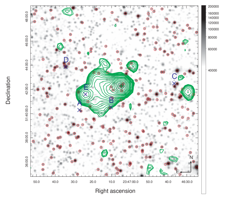
Figure 1: Sky map of the region around 1ES 2344$+$514 (marked by a green cross). Green radio contours at 1.4 GHz are overlaid on an R-band image. IR point sources are indicated by red circles. An “X” and its label mark individual components identified by Chandra (Donato et al. 2003). The logarithmic grey scale shows scaled densities. Radio contours are given from 0.001 Jy/beam to 0.241 Jy/beam in 20 logarithmically scaled steps. Only IR sources of J magnitude $<15$ are displayed. Data reference: X-rays: Donato et al. (2003); optical: DSS2red; IR: 2MASS; radio: NVSS, obtained from NED.

To date, 1ES 2344$+$514 has been studied in only one MW campaign that included gamma-ray observations, conducted by RXTE, Swift and VERITAS (Acciari et al. 2011b). Giommi et al. (2012) reported Planck, Swift and Fermi observations, covering energies from radio to GeV, but detecting the source only in the UV and X-ray bands. In this paper we present the first simultaneous radio to VHE gamma-ray observations of 1ES 2344$+$514. The campaign was organised independently of the flux state to allow investigations of a low, possibly “quiescent”, state of the source. The observations were scheduled to give the best simultaneous coverage between the different instruments, with less than a day time difference between VHE, X-ray and optical bands. The time delays with respect to radio observations were longer due to the longer variability time scale in this energy regime. The campaign took place in late 2008 shortly after the launch of the Fermi satellite. In total six radio observatories contributed, including VLBA imaging of the source in several frequency bands. 1ES 2344$+$514 was monitored in the optical R-band by the CrAO, KVA and Tuorla telescopes, in ultraviolet and X-rays by Swift UVOT and XRT and in high energy (HE) gamma rays by AGILE and Fermi. The core part of the campaign was centred around the MAGIC VHE gamma-ray observations of the source. Parts of the MW data sets have been presented in Rügamer et al. (2011a, b). In this paper we present the complete results of the campaign. We adopt a cosmology with $\Omega_{\mathrm{m}}=0.27$, $\Omega_{\Lambda}=0.73$ and $H_{0}=71\;\mathrm{km}\;\mathrm{s}^{-1}\;\mathrm{Mpc}^{-1}$ for calculating radio component linear sizes and proper motions.

The paper is organised as follows: in Sect. 2, we present short descriptions of the various participating instruments, their observations as well as the corresponding data analyses. The results will be shown in Sect. 3 and discussed in Sect. 4 including the spectral energy distributions and the theoretical models. Final remarks are given in Sect. 5.

2 Instruments, Multi-Wavelength Observations and Data Analysis

In this section, the instruments participating in the MW campaign, their observations and data reduction processes will be presented ordered by their wavelength regime. A summary of the observation dates is given in Table 1.

Table 1: Multi-wavelength observations of 1ES 2344$+$514.

Instrument	Band	Observation Date
Effelsberg	radio	56; 78; 106; 155
IRAM	radio	25; 106; 137; 178
Metsähovi	radio	30; 46; 124; 127; 130; 136; 138
OVRO	radio	61 – 179
RATAN-600	radio	29 – 42
VLBA	radio	61 – 62
CrAO	R-band	74; 77; 85; 101; 105; 112; 117
KVA$+$Tuorla	R-band	22 – 134
Swift	UV & X-rays	30; 45 – 84
AGILE	HE gamma rays	70 – 100
Fermi	HE gamma rays	59 – 100
MAGIC-I	VHE gamma rays	59 – 100

2.1 The MAGIC Telescope

The MAGIC (Major Atmospheric Gamma-ray Imaging Cherenkov) project operates a system of two 17-m Imaging Air Cherenkov Telescopes located on the Canary Island of La Palma 2200 m above sea level (Aleksić et al. 2012c). MAGIC has been operating in stereoscopic mode since 2009, accordingly the observations presented in this paper were conducted with MAGIC-I only (mono mode). MAGIC-I had a standard trigger threshold of 60 GeV for observations at low zenith angles, an angular resolution of $\sim$ 0.1^∘ for single events and an energy resolution above 150 GeV of $\sim$ 25 % (for details, see Albert et al. 2008).

MAGIC-I observed 1ES 2344$+$514 from 20/10/2008 to 30/11/2008 at zenith angles between 23^∘ and 31^∘ for a total of 26.4 hours in so-called wobble mode, where the source was displaced by 0.4^∘ from the camera centre in order to allow the recording of simultaneous OFF-source data with the same offset from the camera centre (Daum et al. 1997).

The data were analysed as described in Aleksić et al. (2010) with the exception of the signal arrival time extraction. Instead of determining the arrival time of the signal at the pulse maximum, which was needed at that time due to the special nature of those data, the standard method of determining the signal arrival time at half of the rising flank was used here. 20.8 hours of data survived the quality selection. Background suppression was accomplished by a cut in shower area versus shower SIZE (i.e. total photoelectron content), optimised on 0.7 hours of data from a high state of Mrk 421 taken during the same observing period as 1ES 2344$+$514 and hence with similar data quality and observation conditions. The significance of the signal was determined by a cut in $\theta^{2}$ optimised also on the Mrk 421 data set, where $\theta$ is the angular distance between the expected and reconstructed source position. All significances of the VHE signals given in the following sections were determined by Eq. 17 of Li & Ma (1983) with $\alpha=1/3$, i.e. using 3 OFF regions.

The source spectrum has been derived from events with $\theta^{2}<0.046$ deg², yielding an analysis threshold of $\sim$ 190 GeV. Upper limits (UL) were calculated by applying model 4 of Rolke et al. (2005) using a confidence level (c.l.) of 95 %. The conversion from the differential spectrum to spectral energy density $\nu F_{\nu}$ has been accomplished by multiplying the differential flux with the energy of the Lafferty-Wyatt bin centre (Lafferty & Wyatt 1995) squared.

The MAGIC analysis results presented here were confirmed by an independent internal analysis.

2.2 The AGILE Satellite

AGILE (Astrorivelatore Gamma ad Immagini LEggero) (Tavani et al. 2009) is a scientific mission of the Italian Space Agency dedicated to the observation of astrophysical sources of high energy gamma rays in the 30 MeV – 50 GeV energy range, with simultaneous X-ray imaging capability in the 18 – 60 keV band. AGILE is the first high-energy mission which makes use of a silicon detector for the gamma ray to pair conversion. The AGILE payload combines for the first time two coaxial instruments: the Gamma-Ray Imaging Detector (GRID, composed of a 12-planes Silicon-Tungsten tracker, a Cesium-Iodide mini-calorimeter and the anti-coincidence shield) and the hard X-ray detector Super-AGILE. The use of the silicon technology provides good performance of the gamma ray GRID imager in a relatively small and compact instrument: an effective area of the order of 500 cm² at several hundred MeV, an angular resolution of around 3.5^∘ at 100 MeV, decreasing below 1^∘ above 1 GeV, a very large field of view ($\sim$ 2.5 sr) as well as accurate timing, positional and attitude information.

During the period 07/2007 – 10/2009, AGILE was operated in “pointing observing mode”, characterised by long observations called Observation Blocks (OBs), typically of two to four weeks duration, mostly concentrated along the Galactic plane. Since 11/2009 the satellite has been operating in “spinning observing mode”, surveying a large fraction (about 70 %) of the sky each day. The time period covered by the 2008 MW campaign includes the AGILE OB 6400, publicly available from the ASDC Multimission Archive web page. 1ES 2344$+$514 was observed by AGILE at $\sim$ 40^∘ off-axis from the mean pointing direction in the time window 31/10/2008 to 30/11/2008.

AGILE-GRID data from the official Processing Archive (SPINNING sw = 5_21_18_19 and POINTING sw = 5_19_18_17), obtained by using the AGILE Standard Analysis Pipeline (Pittori et al. 2009), were analysed using the latest scientific software (AGILE_SW_5.0_SourceCode) and in-flight calibrations (I0023) publicly available since 30/09/2011 at the ASDC site. Counts, exposure, and Galactic background gamma-ray maps were created with a bin-size of 0.3${}^{\circ}\times 0.3^{\circ}$, for $E>100$ MeV, selecting only events flagged as confirmed gamma-ray events. Events collected during passages of the South Atlantic Anomaly or whose reconstructed directions form angles with the satellite-Earth vector smaller than 90^∘ were rejected to avoid Earth albedo contamination. In order to derive the estimated flux (or flux upper limits) of the source we ran the AGILE point source analysis software based on the maximum likelihood technique using a radius of 10^∘.

2.3 Fermi-LAT

The Fermi satellite started taking official science data on 4/08/2008 (Atwood et al. 2009). Two different detectors are on board: the Gamma-ray Burst Monitor (GBM), sensitive at low energies (8 keV – 40 MeV), and the Large Area Telescope (LAT), sensitive at high energies (20 MeV – $>300$ GeV).

Typically, the Fermi satellite is rocked first towards the north pole of the orbit and then, in the next orbit, towards the south, alternating in this way the pointing in every orbit. This main operating mode, called “All-Sky scanning mode”, allows for full sky coverage every two orbits, or three hours.

The LAT is a large field of view ($\sim$ 2.4 sr) electron-positron pair conversion telescope made up of a high-resolution silicon microstrip tracker, a CsI hodoscopic electromagnetic calorimeter and an anti-coincidence detector for the identification of charged particle backgrounds. The full description of the instrument and its performance can be found in Atwood et al. (2009). The LAT point spread function (PSF) depends strongly upon the energy of the impinging gamma ray and on the depth of the conversion point in the tracker, and mildly upon the incidence angle. For normal-incidence conversions in the upper section of the tracker, the PSF 68 % containment radius is 0.6^∘ for 1 GeV photons and amounts to $\sim$ $0.04^{\circ}$ above 100 GeV.

The Fermi-LAT data for 1ES 2344$+$514 presented here were obtained in the time period between 20/10/2008 22:35:00 UTC and 30/11/2008 21:31:00 UTC coordinated with the observations with MAGIC. The data have been analysed by using the standard Fermi-LAT Science Tools software package, version 09-27-01 as described in the Cicerone website. The Pass 7 Source event class and P7SOURCE_V6 instrument response functions (Atwood et al. 2009) were used in our analysis. We selected events in a region of interest (RoI) centred on the source position within $15^{\circ}$, having an energy between 100 MeV and 300 GeV. In order to avoid background contamination from the bright Earth limb, time intervals when the Earth entered the LAT RoI were excluded from the data set. In addition, events with zenith angles larger than $100^{\circ}$ with respect to the Earth reference frame (Abdo et al. 2009a) were excluded from the analysis. The data were analysed with an unbinned maximum likelihood technique, described in Mattox et al. (1996), using the analysis software (gtlike) developed by the LAT team and described in the Cicerone website mentioned above. The fitting procedure maximises the likelihood acting simultaneously on the free spectral parameters for the source of interest, those of nearby gamma-ray sources and the diffuse backgrounds, modelled using ring_2year_P76_v0 for the Galactic diffuse emission and isotrop_2year_P76_source_v0 for the extragalactic isotropic emission models. To maintain comparability, photon fluxes were converted to spectral energy densities applying the same method as used for AGILE.

In addition we also performed a dedicated analysis of the highest energy photons ($>100$ GeV) detected from 1ES 2344$+$514 within the first 44 months of LAT operation. Only events of the purest class (Pass_7_V6_Ultraclean) from a 68 % containment radius around the direction of the source were considered for this analysis. Front and back photons, accordingly to the definition in Atwood et al. (2009), were treated separately, having a different distribution of the PSF. Since no results on such events over this long time scale have been reported in literature, the analysis has been applied to four additional TeV HBLs with a comparable redshift (Mrk 421, Mrk 501, Mrk 180 and 1ES 1959$+$650).

2.4 Swift

The Swift satellite (Gehrels et al. 2004) is equipped with three telescopes, the Burst Alert Telescope (BAT; Barthelmy et al. 2005) which covers the 14 – 195 keV energy range, the X-ray telescope (XRT; Burrows et al. 2005) covering the 0.2 – 10 keV energy band, and the UV/Optical Telescope (UVOT; Roming et al. 2005) covering the 180 – 600 nm wavelength range with V, B, U, UVW1, UVM2 and UVW2 filters.

Swift XRT observed 1ES 2344$+$514 from 09 – 11/2008 with a total of 21 exposures (see Table 6) with exposure times ranging from 200 s to 5 ks. The two exposures lasting well below 1 ks were too short for deriving a flux and were therefore excluded from the analysis. The XRT data were processed with standard procedures using the FTOOLS task XRTPIPELINE (version 0.12.6) distributed by HEASARC within the HEASOFT package (v.6.10). Events with grades 0 – 12 were selected (see Burrows et al. 2005) and latest response matrices available in the Swift CALDB (v.20100802) were used. For the spectral analysis the source events were extracted in the 0.3 – 10 keV range within a circle with a radius of 20 pixels ($\sim$ 47″). The background was extracted from an off-source circular region with a radius of 40 pixels. The spectra were extracted from the corresponding event files and binned using GRPPHA to ensure a minimum of 25 counts per energy bin, in order to guarantee reliable $\chi^{2}$ statistics (Gehrels 1986). Spectral analyses were performed using XSPEC version 12.6.0. The spectral index was determined using an absorbed power law fit ($f_{0}\cdot E^{-\alpha}\cdot\mathrm{e}^{-\tau}$) from 0.3 – 10 keV, with the absorption $\tau$ being the product of the absorption hydrogen-equivalent column density N_H and the element-specific energy-dependent photoelectric cross section $\sigma\left(E\right)$. N_H was fixed to the Galactic value in the direction of the source of $1.5\cdot 10^{21}\,\mathrm{cm}^{-2}$ (Kalberla et al. 2005). Not fixing this parameter, the XRT data analysis yields a value of $\left(2.0\pm 0.2\right)\cdot 10^{21}\,\mathrm{cm}^{-2}$. Since some daily data sets showed hints of spectral curvature, also fits using a log-parabola model ($f_{0}\cdot E^{-\left(a+b\log_{10}\left(E\right)\right)}\cdot\mathrm{e}^{-\tau}$) were performed. However, for the majority of the cases the log-parabola fit was not significantly preferred by a logarithmic likelihood ratio test over the simple power law model (see Table 6). Therefore, the simple power law results were used as a common basis.

For the long-term source evolution, 67 observations of 1ES 2344$+$514 between 2005 and 2010 were analysed. A slightly different analysis procedure was used compared to the MW data reduction. The spectra were determined using XSELECT (V2.4b) to extract events with an energy of 0.5 – 10 keV from the corresponding event files. The background was deduced from an annulus around the source with an inner radius of 50 pixels ($\sim$ 118″) and an outer radius of 70 pixels ($\sim$ 165″). Spectral analysis and binning was performed in ISIS (V 1.6.2-3), where a minimum signal to noise ratio of 5 was required for grouping the data. The spectral index was determined in the range 0.5 – 10 keV using an absorbed power law fit. To calculate the integral flux the photon flux was evaluated on a fine grid between 2 and 10 keV. The neutral hydrogen-equivalent column density was determined for each spectrum from the spectral fit, yielding for spectra with a d.o.f. $>35$ a mean value of $\left(1.71\pm 0.14\right)\cdot 10^{21}$ cm^-2. Flux errors are given at a 90 % confidence level. The event counts for calculating the hardness ratios for the MW data were extracted applying this pipeline in the full energy range.

Swift UVOT observed the source with all filters (V, B, U, UVW1, UVM2, UVW2) each time. The source counts were extracted from a circular region 5 arcsec-sized centred on the source position, while the background was extracted from a larger circular nearby source-free region. These data were processed with the uvotmaghist task of the HEASOFT package. The observed magnitudes have been corrected for Galactic extinction $E_{\mathrm{B-V}}=0.191$ mag (Schlafly & Finkbeiner 2011) using the extinction curve from Fitzpatrick (1999) adopting $R_{\mathrm{V}}=3.07$ (McCall & Armour 2000). The host-galaxy flux contributes significantly to the observed brightness in the V-, B- and U-bands, however no values for the contribution were found in the literature. Therefore, the contribution is estimated from the R-band value from Nilsson et al. (2007) (aperture 5″) using the galaxy colours at $z=0$ from Fukugita et al. (1995) resulting in $\mathrm{V}=\left(1.96\pm 0.16\right)$ mJy, $\mathrm{B}=\left(0.95\pm 0.20\right)$ mJy and $\mathrm{U}=\left(0.22\pm 0.20\right)$ mJy. In these bands the host galaxy contributes $\sim$ 80 – 90 % to the measured flux and additionally the uncertainty of the host-galaxy contribution is rather large. Therefore these bands are not considered for spectral energy distribution modelling.

The magnitudes measured in the UV filters were converted to units of $\mathrm{erg}\,\mathrm{cm}^{-2}\,\mathrm{s}^{-1}$ using the photometric zero points as given in Breeveld et al. (2011) and effective wavelengths and count-rate-to-flux ratios of GRBs from the Swift UVOT CALDB 02 (v.20101130). Raiteri et al. (2010) noted that these ratios are not necessarily applicable to BL Lac objects, due to their different spectrum and a B – V value typically larger than the applicable range. Therefore, they determined the UVOT effective wavelengths and count-rate-to-flux ratios anew (for BL Lacertae, an LBL at $z=0.069$). We compare these values with the ones used in this work and find that the difference amounts to $\lesssim 1$ % for the V, B and U filters. In the case of the UV bands, the effective wavelengths (count-rate-to-flux ratios) are $\sim$ 7 % ($\sim$ 2 %), $\sim$ 3 % ($\sim$ 1 %) and $\sim$ 9 % ($\sim$ 13 %) larger for the UVW1, UVM2 and UVW2 filters, respectively. These differences are smaller than or comparable to the intrinsic errors of the corresponding values with the exception of the UVW2 count-rate-to-flux ratio (intrinsic error of $\sim$ 2 %). Therefore we did not apply a new calibration but increased the error of the UVW2 count-rate-to-flux ratio from $\sim$ 2 % to 13 % to account for a potential change in this value as large as found by Raiteri et al. (2010). However the actual uncertainty should be much below that, considering that some (if not most) of the difference between the ratios arises solely from using new effective wavelengths, which is not the case in this work.

Swift BAT operates in full sky mode. The BAT data of 1ES 2344$+$514, taken from the 58-Month Catalog, have been re-binned using the tool rebingausslc from the HEASOFT package to weekly (7 days), monthly (30.44 days), quarterly (91.31 days) and yearly (365.24 days) bins. The default settings for the bin centre of rebingausslc have been used, no trials have thus been made for selecting the binning. Integral fluxes were calculated according to Tueller et al. (2010) by multiplying the Crab-normalised count rate of 1ES 2344$+$514 with the Crab flux measured in the same time interval and energy band. These fluxes were then converted to spectral energy densities in each energy band at the Lafferty-Wyatt bin position (Lafferty & Wyatt 1995) assuming a simple power law with a spectral index of 2.62 as given in the BAT 58-Month Catalog.

2.5 KVA and Tuorla

1ES 2344$+$514 has been monitored in the optical R-band by the Tuorla Blazar Monitoring Program since 2002. The observations are done using the Tuorla 1-m telescope (Finland) and the Kungliga Vetenskapsakademien (KVA) 35-cm telescope (La Palma). The latter can be controlled remotely from the Tuorla Observatory. In the following, “KVA” will be used as a synonym for “KVA$+$Tuorla”. The source is typically observed a few times per week, but during the Swift pointings mechanical problems prevented KVA observations. The photometric measurements are made in differential mode, i.e. by obtaining CCD images of the target and calibrated comparison stars in the same field of view (Fiorucci et al. 1998). The magnitudes of the source and comparison stars are measured using aperture photometry and the (colour corrected) zero point of the image determined from the comparison star magnitudes. The object magnitude is computed using the zero point and a filter-dependent colour correction. Magnitudes are then transferred to linear flux densities using the formula $F=F_{0}\cdot 10^{\mathrm{mag}/-2.5}$, where mag is the magnitude of the object and $F_{0}$ is a filter-dependent zero point (in the R-band the value $F_{0}=3080$ Jy is used from Bessell 1979).

Since 1ES 2344$+$514 has a bright host galaxy and a nearby star that contributes to the observed flux, these contributions have to be removed in order to derive the core flux for the spectral energy distribution. Nilsson et al. (2007) determined these contributions which depend on seeing and the aperture used for the measurement. Since all observations for this campaign were done with constant aperture (7.5″) and in similar seeing conditions, we subtract a constant value of $\left(3.70\pm 0.05\right)$ mJy.

2.6 CrAO

Observations from the Crimean Astrophysical Observatory (CrAO) were obtained with the AZT-11 telescope and an FLI IMG1001E CCD camera, through an R-band filter. Differential photometry was performed between the blazar and published comparison stars on the same CCD frame. The comparison stars and apertures used were the same as for KVA. The resulting magnitudes were converted to mJy using the standard formula. The CrAO flux densities were found to be $\sim$ 12 % lower than the KVA points and were shifted by a fixed value ($\sim$ 0.49 mJy) to match the KVA observations. The corresponding shift has been deduced from the average flux density difference between both telescopes for nights with an observation time difference $<0.3$ days. Two out of seven data point pairs satisfied this condition. A difference of $\sim$ 10 % is expected due to CrAO using the Johnson R-band filter whereas KVA is measuring in the Cousins R-band filter.

2.7 Effelsberg 100-m and IRAM 30-m Radio Telescopes

Quasi-simultaneous cm-to-mm radio spectra have been obtained within the framework of a Fermi related monitoring program of gamma-ray blazars, namely the F-GAMMA program (Fuhrmann et al. 2007; Angelakis et al. 2008). The total frequency range spans from 2.64 GHz to 228.4 GHz using the Effelsberg 100-m and IRAM 30-m telescopes. The millimetre observations are closely coordinated with the more general flux monitoring conducted by IRAM, and observations of both programs are included in this paper. 1ES 2344$+$514 has been observed in late 2008 once a month with these facilities.

The Effelsberg measurements were conducted with the secondary focus heterodyne receivers at 2.64, 4.85, 8.35, 10.45, 14.60, 23.05, 32.00 and 43.00 GHz. The observations were performed quasi-simultaneously with “cross-scans” (that is, slewing over the source position in azimuth and elevation direction), with an adaptive number of sub-scans for reaching the desired sensitivity (for details see Fuhrmann et al. 2008; Angelakis et al. 2008). Subsequently, pointing off-set corrections, gain corrections and atmospheric opacity corrections have been applied to the data. The conversion to Jy has been done using the standard calibrators: 3C 48, 3C 161, 3C 286, 3C 295 and NGC 7027. The standard deviation of the flux calibrators amounts to $<5$ % at 43.00 GHz and $<1$ % at 2.64 GHz. The Effelsberg error bars are given including systematic uncertainties.

IRAM (Institut de Radioastronomie Millimétrique) operates a 30-m radio telescope located on Pico Veleta near Granada in Spain. The IRAM observations of 1ES 2344$+$514 and primary/secondary calibrators were carried out with calibrated cross-scans using the receivers operating at 86.2 and 142.3 GHz, occasionally also at 228.4 GHz. The opacity corrected scans were converted into the standard temperature scale and finally corrected for small remaining pointing offsets and systematic gain-elevation effects. The conversion to the Jy flux density scale was done using the instantaneous conversion factors derived from the frequently observed primary (Mars, Uranus) and secondary (W3(OH), K3-50A, NGC 7027) calibrators.

2.8 Metsähovi 14-m Radio Telescope

The 37 GHz observations were conducted with the 13.7-m diameter Metsähovi radio telescope, which is a radome-enclosed paraboloid antenna in Finland. The measurements were made with a 1 GHz-band dual beam receiver centred at 36.8 GHz. The HEMPT (high electron mobility pseudomorphic transistor) front end operates at room temperature. The observations are ON – ON observations, alternating the source and the sky in each feed horn. A typical integration time to obtain one flux density data point is between 1200 and 1400 s. The detection limit of the telescope at 37 GHz is of the order of 0.2 Jy under optimal conditions. Data points with a signal to noise ratio $<4$ are considered as non-detections.

The flux density scale is set by observations of DR 21. The sources NGC 7027, 3C 274 and 3C 84 are used as secondary calibrators. A detailed description of the data reduction and analysis is given in Teräsranta et al. (1998). The error estimate in the flux density includes the contribution from the measurement rms and the uncertainty of the absolute calibration.

2.9 OVRO 40-m Radio Telescope

Regular 15.0 GHz observations of 1ES 2344$+$514 were carried out as part of a high-cadence gamma-ray blazar monitoring program using the Owens Valley Radio Observatory (OVRO) 40-m telescope (Richards et al. 2011). This program, which commenced in late 2007, now includes about 1600 sources, each observed with a nominal twice per week cadence. Data during the beginning of this MW campaign were unavailable due to a hardware outage. The OVRO 40-m results used in this paper span the period 22/10/2008 to 11/02/2012.

The OVRO 40-m uses off-axis dual-beam optics and a cryogenic high electron mobility transistor (HEMT) low-noise amplifier with a 15.0 GHz centre frequency and 3 GHz bandwidth. The total system noise temperature is about 52 K, including receiver, atmosphere, ground, and CMB contributions. The two sky beams are Dicke-switched using the off-source beam as a reference, and the source is alternated between the two beams in an ON – ON fashion to remove atmospheric and ground contamination. A noise level of approximately 3 – 4 mJy in quadrature with about 2 % additional uncertainty, mostly due to pointing errors, is achieved in a 70 s integration period. Calibration is achieved using a temperature-stable diode noise source to remove receiver gain drifts. The flux density scale is derived from observations of 3C 286 assuming a value of 3.44 Jy at 15.0 GHz (Baars et al. 1977). The systematic uncertainty of about 5 % in the flux density scale is not included in the error bars. Complete details of the reduction and calibration procedure are found in Richards et al. (2011).

2.10 RATAN-600

The radio spectrum of 1ES 2344$+$514 was observed with the 600-m ring radio telescope RATAN-600 (Korolkov & Pariiskii 1979) of the Special Astrophysical Observatory, Russian Academy of Sciences, located in Zelenchukskaya, Russia, from 20/09/2008 to 03/10/2008. The continuum spectrum was measured six times quasi-simultaneously (within several minutes) in a transit mode with six different receivers at the following central frequencies (and frequency bandwidths): 0.95 GHz (0.03 GHz), 2.3 GHz (0.25 GHz), 4.8 GHz (0.6 GHz), 7.7 GHz (1.0 GHz), 11.2 GHz (1.4 GHz), 21.7 GHz (2.5 GHz). Due to radio frequency interference, we were unable to detect the source at the two longest wavelengths. An average spectrum of the six independent 5 – 22 GHz measurements is presented in this paper. Details on the method of observation, data processing, and amplitude calibration are described by Kovalev et al. (1999). The data were collected using the southern sector with the Flat reflector.

2.11 VLBA

1ES 2344$+$514 was observed with the VLBA (Napier 1995) on 23/10/2008 at 4.6, 5.0, 8.1, 8.4, 15.4, 23.8 and 43.2 GHz in the framework of a survey of parsec-scale radio spectra of 20 gamma-ray bright blazars (Sokolovsky et al. 2010b). The observations were conducted with ten on-source scans (each four to seven minutes long depending on frequency) spread over eleven hours. The data reduction was performed in the standard manner using the AIPS package (Greisen 1990). An amplitude calibration procedure similar to the one described in Sokolovsky et al. (2011) was applied, resulting in $\sim$ 5 % calibration accuracy at the 4.6 – 15.4 GHz range and $\sim$ 10 % accuracy at 23.8 and 43.2 GHz. The Difmap software (Shepherd 1997) was used for imaging and modelling of the visibility ($uv$) data. The integrated parsec-scale flux densities were derived by summing all CLEAN (Högbom 1974) components used to represent calibrated visibilities.

1ES 2344$+$514 was also observed with VLBA at 15.4 GHz during the campaign as a part of the MOJAVE (Monitoring Of Jets in Active galactic nuclei with VLBA Experiments) long-term program to monitor radio brightness and polarisation variations in jets associated with active galaxies visible in the northern sky. The data were analysed using the standard procedures (see Lister et al. 2009a, b). Elliptical Gaussian components were used to determine positions and flux densities of individual emission regions within the source. The MOJAVE archive contains two sets of VLBA data on this source at 15.4 GHz. One set contains four epochs published in Piner & Edwards (2004) that span the range 10/1999 to 03/2000. The second consists of ten epochs covering 05/2008 to 11/2010.

3 Results

3.1 Very High Energy Gamma Rays

The MAGIC data analysis yielded a marginal signal of 3.5 $\sigma$ for the complete data set (see Fig. 2 and for detailed results Table 7), which is below the 5 $\sigma$ standard for source discoveries in VHE astronomy. Since 1ES 2344$+$514 is a well-established VHE emitter and the direct environment is lacking suitable alternative source candidates (see Sect.1), we assume that the entire excess comes from the source. The rather long observation time of $\sim$ 20 hours and the fairly large events statistics not dominated by individual features in time makes us confident about the reliability of the signal. Therefore, we derived an average spectrum.

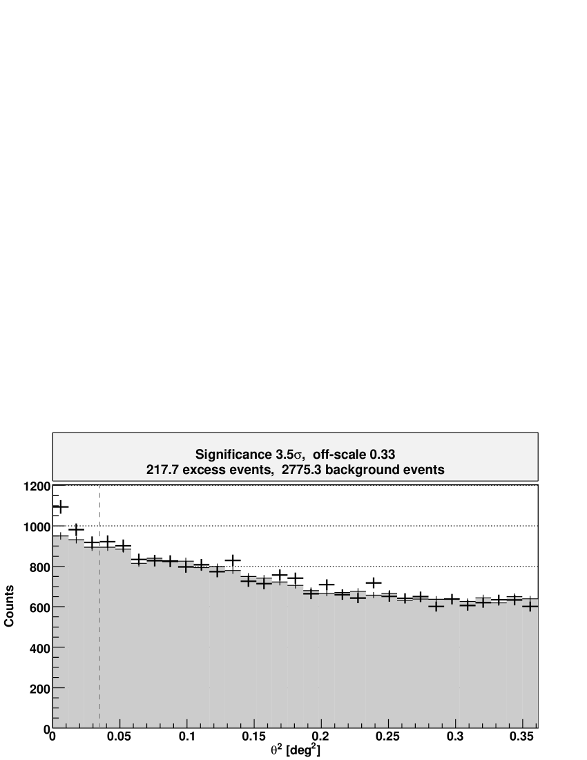
Figure 2: $\theta^{2}$ plot for 1ES 2344$+$514. The vertical dashed line gives the $\theta^{2}$ cut, defining the signal region. The background events are shown by the grey area.

The measured (EBL de-absorbed) spectra are rather well fitted ($\chi^{2}\mathrm{/d.o.f.}=0.36/1$ for both of them; see also the residuals shown in Fig. 3) by a simple power law of the form

$$\frac{\mathrm{d}N}{\mathrm{d}E}=f_{0}\cdot 10^{-12}\,\mathrm{TeV}^{-1}\,\mathrm{cm}^{-2}\,\mathrm{s}^{-1}\cdot\left(E/E_{0}\right)^{-\alpha}$$ (1)

yielding $f_{0}=4.0\pm 1.2$ ($4.8\pm 1.5$) at $E_{0}=0.5$ TeV and $\alpha=2.4\pm 0.4$ ($2.2\pm 0.4$) (see Fig. 3). The given errors are statistical only. We adopt the MAGIC standard systematic errors of 16 % on the energy scale, 11 % on the flux normalisation and $\pm 0.2$ on the spectral index (Albert et al. 2008). The low redshift of the source renders differences between the current extragalactic background light (EBL) models negligible. Here, the effects of EBL absorption were corrected by applying the Kneiske “lower limit” model (Kneiske & Dole 2010).

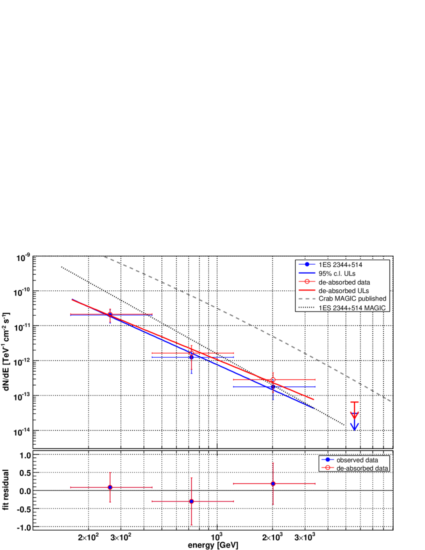
Figure 3: Top panel: Measured (blue, filled circles) and de-absorbed (red, open circles) MAGIC spectra for 1ES 2344$+$514, shown together with the MAGIC 2005 spectrum of 1ES 2344$+$514 (Albert et al. 2007b) as well as the MAGIC Crab spectrum (Albert et al. 2008). Upper limits were derived with a c.l. of 95 %. Bottom panel: Fit residuals defined as the difference between flux and fit divided by the flux value.

No significant variability could be found over the entire observation period on daily time scales, as can be seen from the light curve in Fig. 4 (note that the fluxes are calculated subtracting OFF data from ON data and can therefore become negative) and the flux values given in Table 7. The overall flux $F\left(>170\,\mathrm{GeV}\right)$ amounted to $(7.4\pm 2.1)\cdot 10^{-12}\,\mathrm{ph}\,\mathrm{cm}^{-2}\,\mathrm{s}^{-1}$. A fit with a constant yields a $\chi^{2}\mathrm{/d.o.f.}=19.0/13$, which gives $\sim$ 12 % probability for a constant flux. The low probability arises dominantly from the negative fluctuation around MJD 54767 and the highest flux point at MJD 54787. The latter is indicating a higher state of the source, but since the point is less than 2 $\sigma$ above the fit line, it statistically does not give evidence for variability. The measurements exclude a rise in flux by more than a factor of $\sim$ 9 of the mean flux (derived from the highest 3 $\sigma$ UL calculated for all light curve points), while the peak flux above 300 GeV reported by Acciari et al. (2011b) was a factor of $\sim$ 20 higher than the average flux $F\left(>300\,\mathrm{GeV}\right)=\left(3.4\pm 1.0\right)\cdot 10^{-12}\,\mathrm{ph}\,\mathrm{cm}^{-2}\,\mathrm{s}^{-1}$ found here. Fitting the period-wise light curve, the $\chi^{2}\mathrm{/d.o.f.}=4.0/1$ (probability $\sim$ 5 %), which is still consistent with the hypothesis of a constant flux of the source.

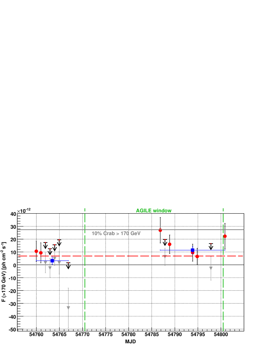
Figure 4: MAGIC light curve of 1ES 2344$+$514 derived from this campaign. The red points give daily fluxes. For points having a flux consistent with or below zero, shown by the grey triangles, 95 % c.l. upper limits were calculated. The red bar on top of each upper limit arrow visualises the bin width. A fit with a constant to all daily flux points is shown by the red dashed line. Additionally, the fluxes for the two observation periods (see also Table 7) are given as blue full squares.

Above 200 GeV, the integral flux amounted to $\left(5.5\pm 1.7\right)\cdot 10^{-12}\,\mathrm{ph}\,\mathrm{cm}^{-2}\,\mathrm{s}^{-1}$, more than a factor 4 lower than the former MAGIC detection (which, at the time, constituted the lowest flux measured of this source at VHE). Compared to the average flux measured by VERITAS $>300$ GeV in 2008 (see Acciari et al. 2011b), the average flux found here is still lower by a factor of $>3$ and hence represents the lowest flux reported from 1ES 2344$+$514 at low VHE thresholds up to now. At high energies the HEGRA collaboration reported a flux $F\left(>970\,\mathrm{GeV}\right)=\left(6.0\pm 1.9\right)\cdot 10^{-13}\,\mathrm{ph}\,\mathrm{cm}^{-2}\,\mathrm{s}^{-1}$ after 72.5 hours of observation time between 1997 and 2002 (Aharonian et al. 2004), which is comparable to our result ($F\left(>970\,\mathrm{GeV}\right)=\left(4.8\pm 3.1\right)\cdot 10^{-13}\,\mathrm{ph}\,\mathrm{cm}^{-2}\,\mathrm{s}^{-1}$).

Previous observations of 1ES 2344$+$514 at VHE confirmed spectral variability, as expected for a BL Lac type object. The spectral index has ranged from $2.43\pm 0.22_{\mathrm{stat}}\pm 0.15_{\mathrm{syst}}$ (Acciari et al. 2011b) to $2.95\pm 0.12_{\mathrm{stat}}\pm 0.2_{\mathrm{syst}}$ (Albert et al. 2007b) with a trend of a hardening of the spectrum with increasing flux. In contrast, the value of $2.4\pm 0.4$ found here indicates a hard spectrum despite a very low flux state. However, these results are still consistent with most of the archival measurements due to the large statistical errors. A hard spectral index would imply that the second SED peak was located at unusually high energies for that flux level, opposite to the spectral hardening trend observed for the best studied blazars (e.g. Mrk 421, Mrk 501, PKS 2155$-$304; Fossati et al. 2008; Albert et al. 2007a; Abramowski et al. 2010).

3.2 High Energy Gamma Rays

AGILE-GRID did not detect the source. The AGILE maximum likelihood analysis using the latest in-flight calibrations yielded a 95 % c.l. UL on the flux above 100 MeV of $3.7\cdot 10^{-8}\,\mathrm{ph}\,\mathrm{cm}^{-2}\,\mathrm{s}^{-1}$ from an effective exposure of $\sim\,2.8\cdot 10^{8}\,\mathrm{cm}^{2}\,\mathrm{s}$ for the MW observation period. Searching for short flares on time scales of seven as well as two days did not yield any detection. Also for the entire period from 07/2007 up to 01/2011, the source was not detected by AGILE. A 95 % c.l. UL on the flux $>100\,\mathrm{MeV}$ of $2.7\cdot 10^{-8}\,\mathrm{ph}\,\mathrm{cm}^{-2}\,\mathrm{s}^{-1}$ was derived, consistent with the 2FGL average flux above 100 MeV which is about $0.9\cdot 10^{-8}\,\mathrm{ph}\,\mathrm{cm}^{-2}\,\mathrm{s}^{-1}$. Given the non-detection of the source we adopt a “standard” spectral photon index of 2.1 for the likelihood analysis.

Fermi-LAT did not detect 1ES 2344$+$514 between 0.1 and 300 GeV during the campaign (effective exposure: $\sim\,3.7\cdot 10^{9}\,\mathrm{cm}^{2}\,\mathrm{s}$). The data were searched for short-time variability on daily and weekly time scales without a clear sign of such. The 2-year Catalog public light curve does not show significant variability on time scales of months around the time of the MW campaign. Upper limits at a 95 % c.l. have been determined applying the standard Bayesian approach for the MW time slot, assuming a spectral index of 2.1 to be consistent with the AGILE calculations. These amount to (in $\mathrm{ph}\,\mathrm{cm}^{-2}\,\mathrm{s}^{-1}$) $3.0\cdot 10^{-8}$ (0.1 – 0.3 GeV), $6.7\cdot 10^{-9}$ (0.3 – 1.0 GeV), $2.7\cdot 10^{-9}$ (1.0 – 3.0 GeV), $8.8\cdot 10^{-10}$ (3.0 – 10 GeV) and $8.6\cdot 10^{-10}$ (10 – 100 GeV).

1ES 2344$+$514 is rather dim for a TeV AGN in the Fermi band. It was detected for the first time after 5.5 months of observations (Abdo et al. 2009b). From the first (1FGL; Abdo et al. 2010) to the second (Nolan et al. 2012) LAT Source Catalog listing, the measured fluxes from 1 – 100 GeV and spectral power law indices changed from $\left(1.40\pm 0.30\right)\cdot 10^{-9}\,\mathrm{ph}\,\mathrm{cm}^{-2}\,\mathrm{s}^{-1}$ to $\left(1.55\pm 0.18\right)\cdot 10^{-9}\,\mathrm{ph}\,\mathrm{cm}^{-2}\,\mathrm{s}^{-1}$ and $1.57\pm 0.12$ to $1.72\pm 0.08$, respectively. These values are consistent within the statistical errors, indicating that the spectral shape did not change significantly on these time scales. Also the monthly light curve shows mostly upper limits and marginal detections without signs of major flares. In fact, only one flux point from the monthly binned Fermi-LAT data is available for 1ES 2344$+$514 within the first nine months of regular measurements, the remaining observations resulted in ULs.

Consequently, 1ES 2344$+$514 seems to be, within the limits of the AGILE-GRID and Fermi-LAT sensitivities, a rather stable and weak source in the HE gamma-ray band over long time scales. Hence, archival data should yield a fairly good estimate of the actual flux during this MW campaign. We therefore use the spectral information from 1FGL on a quasi-simultaneous basis for SED modelling (see Sect. 4.2).

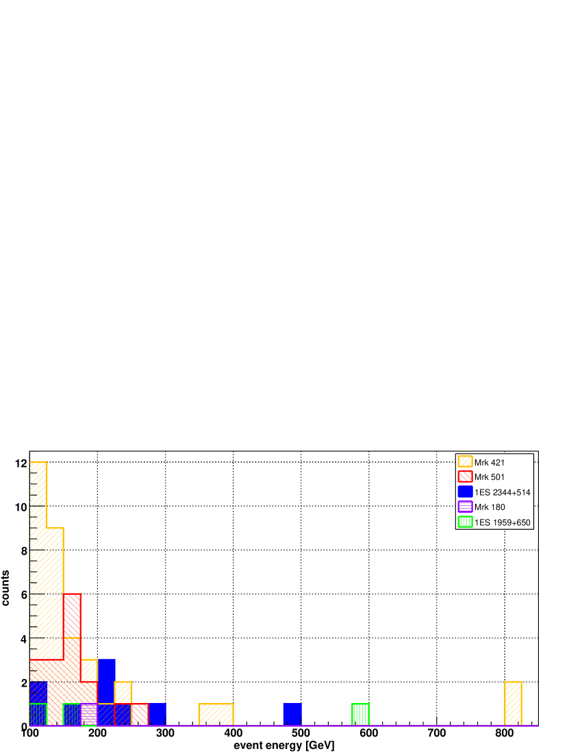
Figure 17: Distribution of events with energies $>100$ GeV detected by Fermi-LAT from Mrk 421, Mrk 501, 1ES 2344$+$514, Mrk 180 and 1ES 1959$+$650.

The LAT high energy analysis revealed nine events with energies in excess of 100 GeV within the first 44 months of operation from 1ES 2344$+$514, the highest energy photon having an energy of nearly 500 GeV (see Table 2). We compare these with the number of events detected from four similar sources (see Sect. 2.3) in Table 8. An investigation of the distribution of event energies is strongly limited by the small event statistics, but judging from Fig. 17, most of them are clustered for Mrk 421 at 100 GeV, whereas the distribution seems to be shifted to $\sim$ 150 GeV for Mrk 501 and $\sim$ 200 GeV for 1ES 2344$+$514. If real, distinct HE flares may be responsible for most of the events $>100$ GeV detected from Mrk 501 and 1ES 2344$+$514 (we note that the events are not clustered in time), in contrast to Mrk 421 for which the distribution indicates a constantly high flux at HE.

The number of events should be correlated directly with the source luminosity. Determining the latter at 60 GeV (from their respective photon fluxes between 10 and 100 GeV in Nolan et al. 2012) and normalising the photon counts to the distance of 1ES 2344$+$514, a linear fit for the five sources yields the expected correlation with a slope of $\left(0.99\pm 0.24\right)$ counts per $10^{43}$ erg s^-1 (not shown). This indicates that the 2FGL fluxes are a suitable representation of the average source behaviour. The goodness of the linear fit is rather low though, having a $\chi^{2}\mathrm{/d.o.f.}=7.4/3$, but is preferred by a logarithmic likelihood ratio test with 98.9 % over a fit with a constant ($\chi^{2}\mathrm{/d.o.f.}=25.5/4$). This is a consequence of the comparably low number of counts from 1ES 1959$+$650, which may arise from the flatter spectral index at HE, and the high number of events detected from 1ES 2344$+$514 (which should be 2 – 3 according to its luminosity). Considering the similar luminosities of the sources, the reason should be a higher flaring duty cycle rather than a higher long-term average flux of the source, which would be in line with the interpretation of the observed shift in event energy distributions. Alternatively, the event counts may also be artificially increased by false identification of Galactic foreground events of 1ES 2344$+$514, being located at a low Galactic latitude of $-9.9^{\circ}$. However, applying the same analysis to two regions containing no HE source at the same Galactic latitude as 1ES 2344$+$514, but 2.5^∘ away from the object, did not result in the detection of any event with energy $>100$ GeV.

The weakness of this investigation is the low statistical basis of only five sources. Additionally, we note that the events above 100 GeV have been extracted from 44 months of observations, whereas the luminosities were determined from 2FGL (24 months). These arguments render our conclusions rather speculative. A catalogue of sources with events $>100$ GeV based on longer observation times is needed to conduct a more reliable study.

Table 2: Fermi-LAT detected events with an energy $>100$ GeV within the first 44 months of operation from the direction of 1ES 2344$+$514 (R.A. 356.77^∘, Dec. 51.71^∘).

MJD	Energy	R.A.	Dec.	Sep.
	[GeV]	[∘]	[∘]	[arcmin]
54879.961	221	356.59	51.80	9
54992.961	174	356.79	51.61	6
55041.439	283	356.73	51.75	3
55358.826	495	356.86	51.63	6
55553.247	201	357.01	51.60	10
55896.009	114	356.79	51.68	2
55702.733	207	356.97	51.63	9
55936.262	107	356.79	51.91	11
55948.736	231	356.74	51.73	2

3.3 X-Rays

Swift XRT detected significant variability (see Fig. 5 and Table 6). The 2 – 10 keV flux increased by $\sim$ 50 % within two days, followed by a slow decline nearly halving the flux during eight days. Thereafter, the flux rose again, showing an irregular behaviour, and eventually reached the highest flux during these observations on the last day. The quicklook Swift XRT intra-day light curves (from the Swift Monitoring Program) did not show significant intra-day variability during the MW campaign.

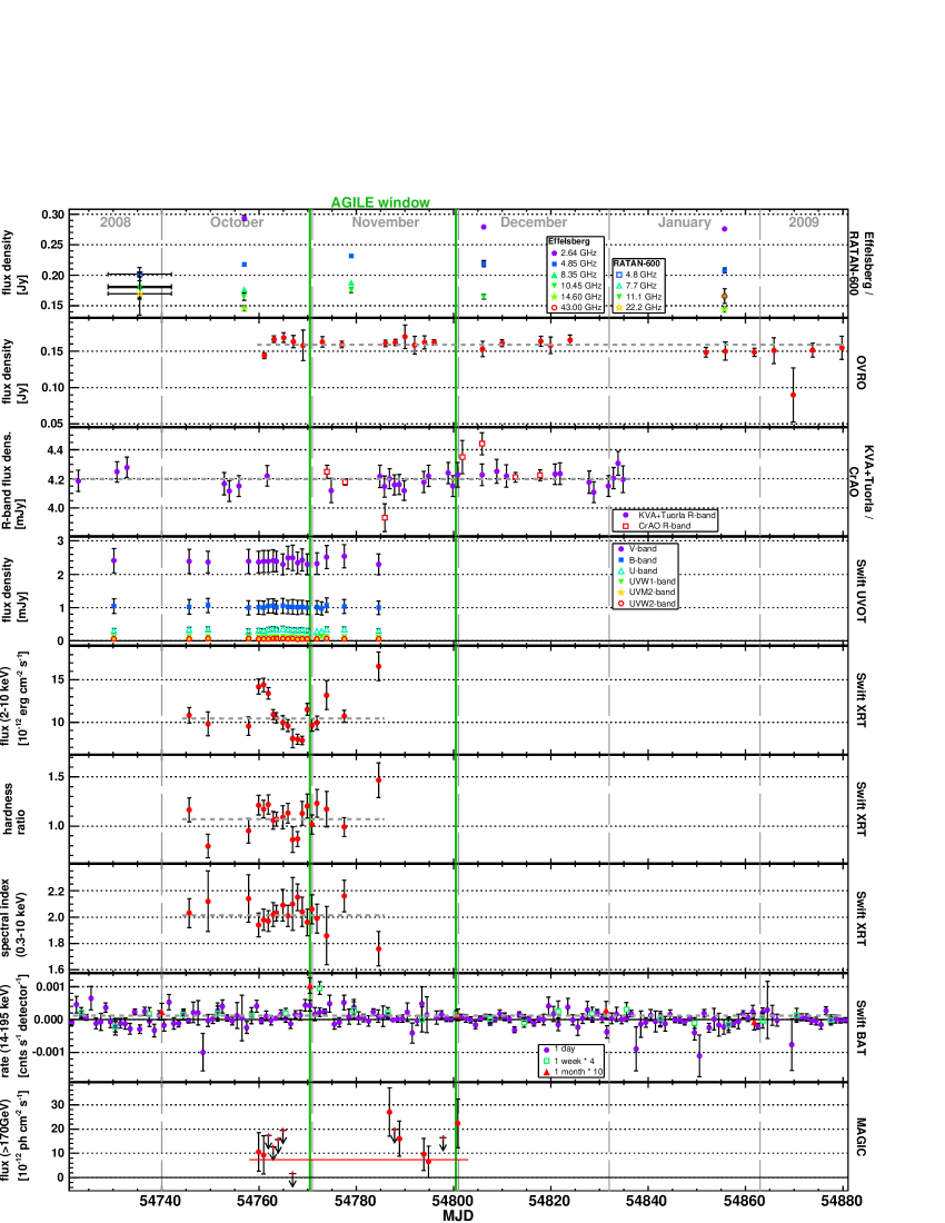
Figure 5: Combined 1ES 2344$+$514 multi-wavelength light curve derived from this campaign. The observation window of AGILE is shown by the vertical solid green lines. Horizontal short-dashed lines represent fits with a constant to the data points. In the R-band, the fit is being applied to the combined KVA and CrAO data points. Hardness ratio is defined as the event counts between 2 – 10 keV divided by the counts between 0.2 – 1 keV. The Swift BAT data are shown for several bin widths some of which have been multiplied by a factor for clarity as indicated in the panel legend. The fit shown in the BAT panel has been calculated for the 1 week binning. One point from the daily BAT light curve (MJD 54867.5, rate $-\left(6.08\pm 3.49\right)\cdot 10^{-3}\,\mathrm{cnts}\,\mathrm{s}^{-1}\,\mathrm{detector}^{-1}$) is not shown for clarity of the plot. The red solid line in the MAGIC panel gives the overall measured flux during the campaign. See text for details.

Compared to previous observations, also the soft X-ray flux was detected at very low levels during this campaign. In Acciari et al. (2011b), the lowest reported X-ray fluxes from 2 – 10 keV by Swift XRT and RXTE PCA were $\left(9.6\pm 0.6\right)\cdot 10^{-12}\,\mathrm{erg}\,\mathrm{cm}^{-2}\,\mathrm{s}^{-1}$ and $\left(9.5\pm 2.6\right)\cdot 10^{-12}\,\mathrm{erg}\,\mathrm{cm}^{-2}\,\mathrm{s}^{-1}$, respectively. The lowest flux in our sample, which was also used to derive the “low state” SED (see Sect. 4.2), is more than 15 % below that level ($\left(7.9\pm 0.5\right)\cdot 10^{-12}\,\mathrm{erg}\,\mathrm{cm}^{-2}\,\mathrm{s}^{-1}$, see Table 6). The source is rather often found in such low flux states between 2 and 10 keV, as further historical measurements show (e.g. $8.4\cdot 10^{-12}\,\mathrm{erg}\,\mathrm{cm}^{-2}\,\mathrm{s}^{-1}$ measured by BeppoSAX in 1998, $9\cdot 10^{-12}\,\mathrm{erg}\,\mathrm{cm}^{-2}\,\mathrm{s}^{-1}$ by Swift in 2005; Giommi et al. 2000; Tramacere et al. 2007), but not below the lowest flux reported here.

The XRT spectral index (determined from a simple power law fit between 0.3 and 10 keV) measured during this campaign varied between $1.76\pm 0.13$ and $2.16\pm 0.12$, a smaller dynamical range compared to previous observations at similar energies (see e.g. Giommi et al. 2000; Acciari et al. 2011b). Despite not being significantly variable over time ($\chi^{2}\mathrm{/d.o.f.}=10.8/18$), there seems to be a dependence of the index on the integral flux, see Fig. 6, which is produced mainly by the highest measured flux point. A linear fit results in a slope of $-\left(2.77\pm 1.11\right)\cdot 10^{-2}$ per $10^{-12}\,\mathrm{erg}\,\mathrm{cm}^{-2}\,\mathrm{s}^{-1}$ with a goodness of fit of 99.9 % ($\chi^{2}\mathrm{/d.o.f.}=4.2/17$), whereas a fit with a constant has a $\chi^{2}\mathrm{/d.o.f.}=10.8/18$ (90.5 %). A logarithmic likelihood ratio test prefers the linear fit with 97.9 %. More meaningful in terms of theoretical models would be to investigate a correlation between the spectral index and the peak position, but because the latter cannot be determined due to lack of significantly curved spectra, the integral flux was used. A negative correlation between flux and spectral index is expected e.g. for an increase of the maximum electron energy in SSC models (e.g. Mastichiadis & Kirk 1997).

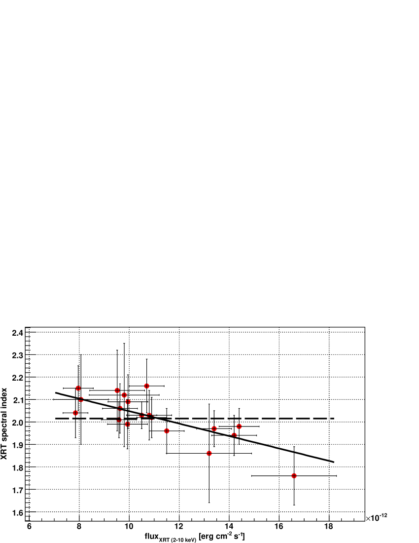
Figure 6: Swift XRT spectral index (determined from a simple power law fit between 0.3 and 10 keV) versus the integral flux for 1ES 2344$+$514 for this campaign. The dashed line shows a fit with a constant, whereas the solid line denotes a linear fit.

The evolution of the hardness ratio (defined here as the ratio of event counts between 2 – 10 keV and 0.2 – 1 keV), another measure of the spectral shape, cannot be described satisfactorily by a constant fit ($\chi^{2}\mathrm{/d.o.f.}=31.6/18$, see Fig. 5). The detected variability allows to test independently if the spectral shape changed considerably with the flux during the observations. Especially during high flux states, the hardness ratio seemed to increase (judging from Fig. 5), which means that the flux rose stronger at higher energies than at lower ones. A weak correlation ($\chi^{2}\mathrm{/d.o.f.}=12.6/17$ for a linear dependence) between the flux and the hardness ratio is visible (see Fig. 7). A constant fit yields a $\chi^{2}\mathrm{/d.o.f.}$ of 31.6/18. Therefore, according to the logarithmic likelihood ratio test, the linear fit is preferred with a confidence of 98.9 %. This finding represents an independent confirmation of the correlation between the spectral index and the flux in Fig. 6 and can be interpreted as the common “harder spectrum when brighter” trend during a blazar flare (see e.g. Pian et al. 1998). From earlier observations, 1ES 2344$+$514 is known to follow such a trend (Giommi et al. 2000; Acciari et al. 2011b).

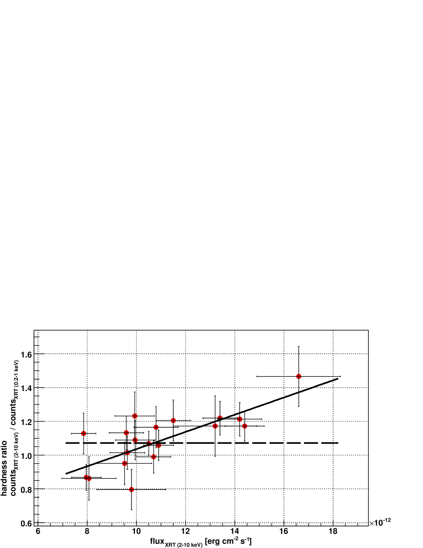
Figure 7: Swift XRT hardness ratio versus integral flux for 1ES 2344$+$514 for this campaign. The dashed line shows a fit with a constant, whereas the solid line denotes a linear fit.

Using only the data during the flare, i.e. from MJD 54757 to 54769, a hint for a counter-clockwise evolution seems to be apparent in the hardness ratio – flux plane (Fig. 8). Kirk et al. (1998) explain such a behaviour in a model where the flare arises from a shock front accelerating electrons within a relativistic jet. A counter-clockwise evolution is visible when the observations happen close to the maximum emission frequency of the electrons, where the acceleration and cooling time scales are comparable. In this case, the electrons will not be accelerated to the highest energies and no related flare at gamma-ray energies is expected. This is in agreement with our simultaneous gamma-ray observations, although our VHE light curve does not exclude the presence of a flare of similar amplitude to have appeared at gamma rays at high confidence. An additional hint for similar cooling and acceleration time scales being responsible for the flare is given by the constant spectral index ($\chi^{2}\mathrm{/d.o.f.}$ of 1.4/10) during the high flux measurements.

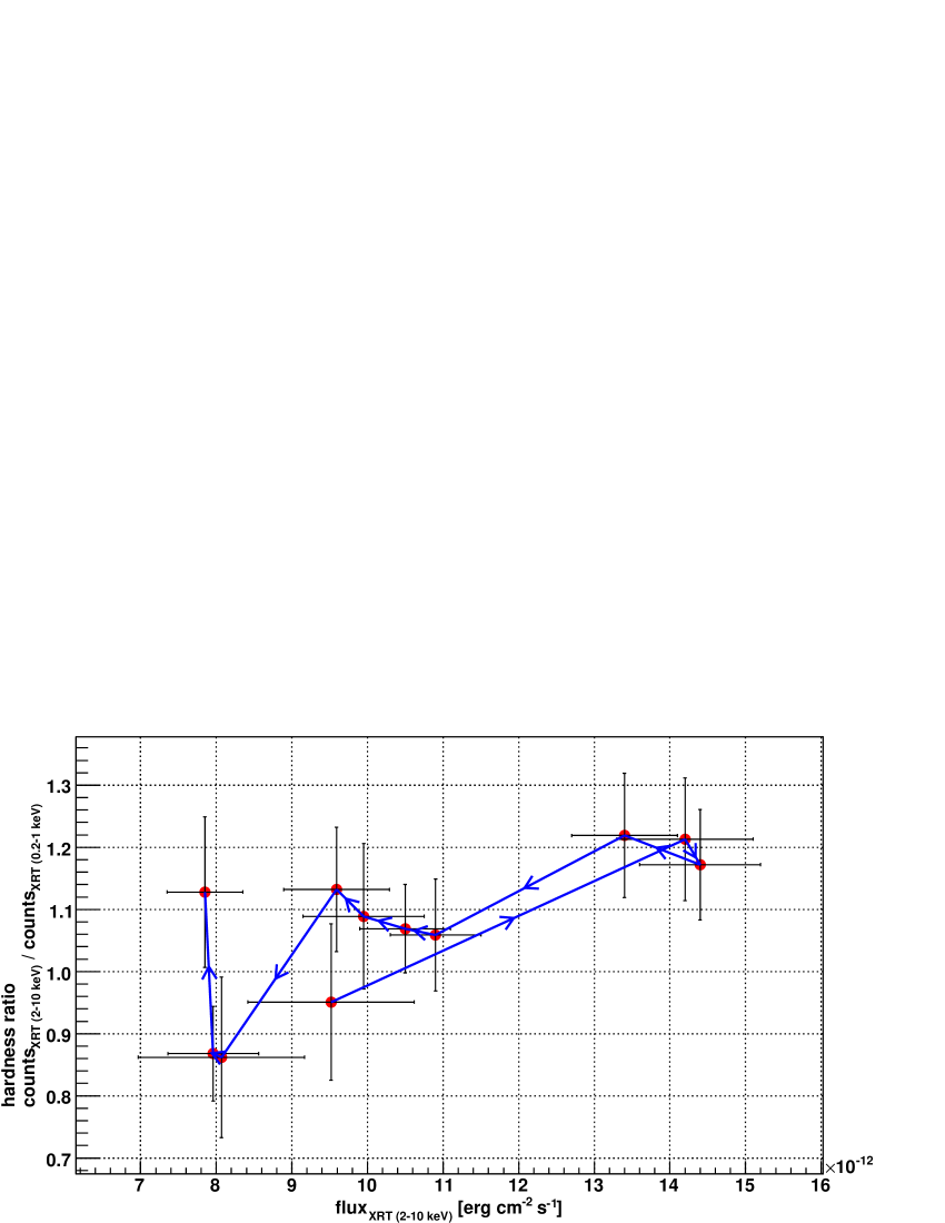
Figure 8: Swift XRT hardness ratio versus integral flux for 1ES 2344$+$514 for the time of the flare (MJD 54757 – 54769). The blue arrows give the evolution in time.

Having found a rather hard spectral index down to $\sim$ 1.8 in the XRT band, the BAT 66 months data have been searched for hints of a signal. Indeed, during the time of XRT observations there are indications of a positive flux for several consecutive days, though insignificant due to limited statistics. Therefore, the daily BAT light curve was re-binned to different time scales (see Sect. 2.4). As can be seen from Fig. 5, variability may be present in the weekly binned data ($\chi^{2}\mathrm{/d.o.f.}=30.3/22$ for a constant flux). The weekly high flux point during the XRT measurements at MJD 54772.5 has a significance of 4.9. However, further analysis shows that this anomalous high flux can be attributed to an artifact of the BAT coded-mask imaging and hence is not believed to be due to any real increase in the emission of 1ES 2344$+$514. For the monthly binned points, the probability of variability increases (constant flux fit: $\chi^{2}\mathrm{/d.o.f.}=12.8/4$). The quarterly and yearly results will be discussed in Sect. 4.1 in the context of the long-term behaviour of the source.

3.4 UV and Optical

KVA found the source on a modest overall flux density level of $\sim$ 4.2 mJy when compared to earlier and later KVA measurements (see also Fig. 14). The host galaxy contribution has not been subtracted for the investigation of the light curves. No significant variability throughout the entire observation period is found in the R-band. The data points are consistent with a constant flux density ($\chi^{2}\mathrm{/d.o.f.}=13.1/29$). The CrAO points are noisier than the KVA points, but all of them are compatible with the KVA data within less than two error bars. Applying a constant fit to the combined KVA$+$CrAO measurements does not provide evidence for variability ($\chi^{2}\mathrm{/d.o.f.}=35.8/36$). The probability for a constant flux slightly increases for all light curves when subtracting the host galaxy contribution. Swift UVOT also did not find significant variability at any of the measured frequencies (see Fig. 5 and Table 9).

3.5 Radio Bands

The results of the measurements at radio frequencies have to be discussed in the light of the different observation techniques. The VLBA interferometer is not sensitive to the steep spectrum extended emission from the large scale jet (expected spectral index: $\sim\,0.5$) but observes directly the flat spectrum of the parsec-scale structure, whereas the single-dish telescopes Effelsberg and OVRO measure the whole jet. As the brightness of the extended components decreases at higher frequencies, the parsec-scale spectrum becomes prominent and the single-dish spectrum becomes flatter with increasing frequency. This is obvious from Fig. 9, comparing the quasi-simultaneous (separated by $\sim$ five days) spectra of Effelsberg$+$OVRO and VLBA. Clearly the VLBA integrated spectrum is much flatter than the Effelsberg$+$OVRO spectrum and can be well fitted by a simple power law of the form $S=\nu^{-\alpha}$, where $S$ is the flux density. The resulting spectral index $\alpha$ is $0.10\pm 0.04$. On the contrary, a simple power law ($\alpha=0.42\pm 0.01$) can not describe the Effelsberg$+$OVRO spectrum sufficiently , judging from the residuals in Fig. 9. A broken power law is clearly preferred, whose fit applied to the Effelsberg$+$OVRO data results in the following parameters: $E_{\mathrm{break}}=\left(5.6\pm 1.0\right)\,\mathrm{GHz}$, $\alpha_{1}=0.49\pm 0.03$, $\alpha_{2}=0.34\pm 0.05$ and a normalisation of $\left(0.153\pm 0.004\right)$ Jy at 10 GHz. $\alpha_{1}$ being close to 0.5 indicates that the emission is dominated by the large scale jet.

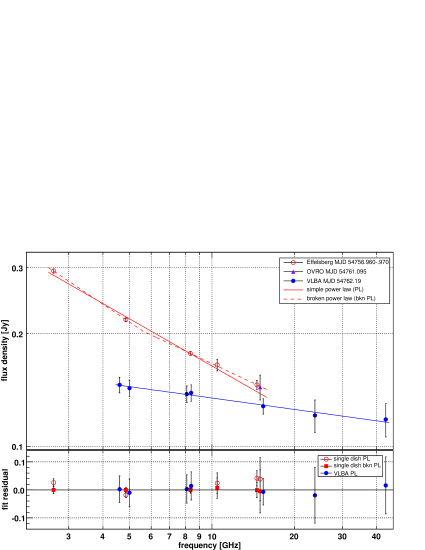
Figure 9: Top panel: Radio spectrum of 1ES 2344$+$514 measured quasi-simultaneously by Effelsberg, OVRO and VLBA. The VLBA points represent integrated flux densities. The solid lines illustrate fits with a simple power law, the dashed line shows a broken power law fit. Bottom panel: Fit residuals, which are the differences between the measured flux densities and the fit values divided by the flux density values. See also footnote 13.

3.5.1 Single-Dish Observations

Single-dish radio observations were conducted from 2.64 GHz (Effelsberg) to 228.39 GHz (IRAM). Since IRAM did not detect the source significantly, 3 $\sigma$ ULs were calculated. The measurements conducted by Effelsberg show significant variability (although of small amplitude) throughout the observations, as can be seen in the top panel of Fig. 5. The flux density was rising first towards MJD 54779.0 at all frequencies (observations at 2.64 GHz were not conducted that day) and declined slowly afterwards. RATAN-600 found the source prior to the Effelsberg observations on a flux density level consistent with the first Effelsberg measurements. The OVRO light curve shows no clear evidence for variability, having a probability of 8.7 % ($\chi^{2}\mathrm{/d.o.f.}=33.9/24$) for a constant flux density. When omitting the outlier around MJD 54870, the probability for a constant flux density is rising to 13.6 %. 1ES 2344$+$514 was too faint to be detected by Metsähovi during the campaign and for 07/10/2008 (MJD 54746), an upper limit on the flux density at 37 GHz of $<0.33$ Jy with S/N $>4$ was calculated. The source was detected by Metsähovi three months earlier at a flux density level of $\left(0.38\pm 0.09\right)$ Jy, which is consistent with the derived upper limit.

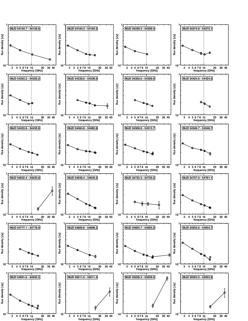
Figure 18: Individual radio spectra of Fig. 10.

To understand the radio behaviour of AGNs, they have to be studied over long periods of time, considering the rather long variability time scales compared to e.g. X-rays. 1ES 2344$+$514 has been observed in the past on a regular basis at radio frequencies. The combined quasi-simultaneous (time difference $<14$ days) radio spectra from Effelsberg, Metsähovi, OVRO and RATAN-600 from 2007 through 2009 are shown in Fig. 10 (for a time-resolved version see Fig. 18). IRAM ULs, where the lowest flux density UL is 0.96 Jy, are not shown for clarity. At frequencies below $\sim$ 20 GHz the source shows steep radio spectra while above this frequency, the spectra become flat or inverted. This is a consequence of high amplitude variability of the mm radio emission, originating from a more compact region than the one dominating the cm-band radio spectrum. These characteristics are in accordance with the model of Angelakis et al. (2012) who demonstrated that the radio spectra of most of the AGNs under study can be described well by a simple two component system consisting of a power-law quiescent spectrum (attributed to e.g. the optically thin diffuse emission of a large scale jet) and a convex synchrotron self-absorbed spectrum (resulting from a recent outburst within the compact region).

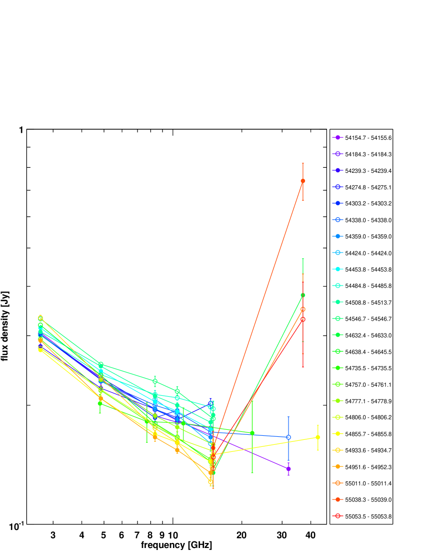
Figure 10: Radio spectra of 1ES 2344$+$514 taken by Effelsberg, Metsähovi, OVRO and RATAN-600 from 2007 through 2009. Data from different instruments have been combined if the time difference was less than 14 days. The thin solid lines simply connect the data points. The legend contains the MJD range of the combined spectra. We recall that the detection limit of Metsähovi at 37 GHz under optimal conditions is $\sim$ 0.2 Jy. See also Fig. 18.

Such an outburst may be explained in the framework of the model of Marscher & Gear (1985) where the emission is coming from a shock propagating in an adiabatic relativistic jet. According to shock models, the feature should move outwards within the jet, i.e. from high to low frequencies. Outbursts are present only at times outside of the principal MW campaign, the most significant one seen by Metsähovi around MJD 55039 having a doubling time of $\lesssim 28$ days and a decline to the original flux density value of $\lesssim 15$ days. IRAM observations two days later provided only unconstraining flux density ULs ($<1.74$ Jy at 86.24 GHz and $<1.95$ Jy at 142.33 GHz), and the quasi-contemporaneous OVRO points, from the flaring day as well as 4, 12 or 15 days after the flare, did not show a significantly higher flux density. However, the flare may have been missed due to the comparably sparse sampling during these days. A fit with a constant to the OVRO data from MJD 55024 until MJD 55054 does not yield significant variability ($\chi^{2}\mathrm{/d.o.f.}=4.9/8$). Hence no conclusions on the validity of the shock scenario can be drawn from this data. However, the time scale of the flare itself is interesting. There are very few examples of such fast variability at 37 GHz for HBLs, e.g. Mrk 421 (Lichti et al. 2008). That is mainly due to their faintness and consequently low detection rate at this frequency. Nevertheless some of these objects are detected at clearly higher flux density values in between periods of non-detections, giving a hint for fast variability (see e.g. Nieppola et al. 2007).

Figure 11 shows the light curve measured by Effelsberg in the context of the F-GAMMA program from beginning of 2007 until mid of 2009 (MJD 54155 – 54952). Apart from an overall higher flux density state especially at high frequencies from the start of the observations until mid of 2008 ($\sim$ MJD 54600), several structures are visible, which reveal an ambivalent correlation during the variability. On the one hand, there are features where only near-by frequency bands showed the same trends with gradually decreasing tendency (MJDs 54239, 54486 and $\sim$ 54935). On the other hand, structures may have been present at all measured bands with about the same strength (MJDs $\sim$ 54547 and $\sim$ 54779). The different features are possibly attributed to re-acceleration of particles within the jet. The occurrence of an equal amplitude at all frequencies or gradually decreasing amplitude with frequency can be explained in that context by different physical conditions within the jet, e.g. a change of the magnetic field or the particle density. Alternatively, the sparse sampling in combination with frequency-dependent time lags may explain some of the observed features.

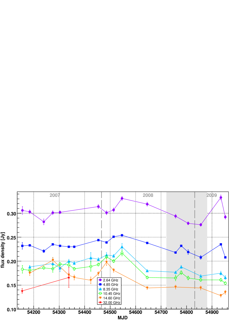
Figure 11: Light curve of 1ES 2344$+$514 measured by Effelsberg. The solid lines connect the points for illustrative purposes. The MW campaign duration is visualised by the grey box.

The probability that the flux density seen by OVRO was constant during the second Effelsberg high state, between MJD 54761 and 54796, is rather low ($\chi^{2}\mathrm{/d.o.f.}=21.2/12$, i.e. $\sim$ 4.8 %), due to the first measurement in this time period (see also Fig. 5). Neglecting this point, the $\chi^{2}\mathrm{/d.o.f.}=2.8/11$, giving highly significant evidence for constancy. The flux density rose from the first point within two days by $\sim$ 16% and remained constant afterwards. This indicates that the peak seen in the Effelsberg light curve around MJD 54779 was indeed a broad high flux density plateau. From the OVRO variability time scale, the Doppler factor can be estimated to be $>3.4$ using Eqs. (1) and (2) in Lähteenmäki & Valtaoja (1999). It should be noted that this estimation method has not been tested for faint radio sources like TeV BL Lacs, and that the estimation of the flare rise time is based on two data points only. Therefore, the value is not representative, but also not in disagreement with the quasi-simultaneous results from the high state SED modelling (see Sect. 4.2).

3.5.2 Interferometric Observations

The VLBA image of 1ES 2344$+$514 (Fig. 12) reveals a core-dominated structure with a smooth jet extending in South-East direction. At the distance of 1ES 2344$+$514 ($z=0.044$), the linear scale of the images is 0.9 pc/mas. The integrated parsec-scale radio spectrum is flat, which is typical for blazars. The VLBA data can be used to estimate the radio core size (the compact feature at the North-Western end of the jet in Fig. 12) at each frequency (see Table 3) by modelling it with a circular Gaussian emission component. At the highest and lowest frequency the core size can only be constrained to $<0.13\,\mathrm{mas}$, i.e. $R\lesssim 10^{17}$ cm, while at the other frequencies the core is resolved. The limiting resolution and component size uncertainties were estimated following Fomalont (1999), Lobanov (2005) and Kovalev et al. (2005).

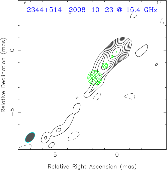
Figure 12: Naturally weighted CLEAN image of 1ES 2344$+$514 obtained with the VLBA on 23/10/2008 (MJD 54762) at 15.4 GHz. Green circles mark positions and sizes of model components listed in the Table 10 from North-West to South-East: the Core, C 3, C 2, C 1. 1 mas corresponds to 0.9 pc in absolute length. Contour image parameters: $\mathrm{peak}=0.11$ Jy/beam, $\mathrm{beam}=0.98\times 0.58$ mas at $\mathrm{PA}=-42.2^{\circ}$, first $\mathrm{contour}=0.50$ mJy/beam, contour level increase $\mathrm{factor}=2$. The naturally weighted beam is shown at the lower left corner of the image.

Table 3: Core size as a function of frequency $\nu$. Errors are given with 1 $\sigma$.

$\nu$	Flux Density	Size	Resolution Limit
[GHz]	[Jy]	[mas]	[mas]
4.6	$0.094\pm 0.006$	$<0.13$	0.13
5.0	$0.091\pm 0.005$	$0.16\pm 0.09$	0.10
8.1	$0.094\pm 0.005$	$0.09\pm 0.06$	0.06
8.4	$0.096\pm 0.005$	$0.14\pm 0.05$	0.06
15.4	$0.102\pm 0.007$	$0.07\pm 0.04$	0.05
23.8	$0.076\pm 0.005$	$0.03\pm 0.02$	0.03
43.2	$0.120\pm 0.022$	$<0.06$	0.06

The source is highly core dominated at parsec scales. Specifically, on the basis of modelling of VLBI data we can estimate that the emission from the core region at 5 GHz accounts for $\sim$ 65 % of the total VLBI flux density progressively increasing up to $\sim$ 75 % at 23.8 GHz. Fast variations with rms values typically well below 10 % in total flux density have been measured at cm wavelengths in a large sample of flat-spectrum compact radio sources (e.g., Kraus et al. 2003; Lovell et al. 2008) – most probably due to scintillation in the Galactic interstellar medium.

The flat parsec-scale radio spectrum showing no clear signs of the synchrotron self-absorption turnover at low frequencies (see Fig. 9) may be explained as optically thin synchrotron emission from an ensemble of electrons having a very hard energy spectrum $N(E)\propto E^{-X}$ (Sokolovsky et al. 2010b). However, the more likely explanation is that the flat spectrum is a result of optically thick synchrotron emission from a Blandford & Königl (1979) type jet. This explanation is supported by the observed core size increase at lower frequencies (Unwin et al. 1994, see Table 3) and the difference in separation between the component C 3 and the core observed at 15.4 (Piner & Edwards 2004) and 43.2 GHz (Piner et al. 2010). Together, these points agree with the standard interpretation of the parsec-scale radio core in 1ES 2344$+$514 as a surface in a continuous Blandford & Königl (1979) jet at which the optical depth at a given frequency $\nu$ is $\tau_{\nu}\simeq 1$ (Lobanov 1998; Sokolovsky et al. 2011). This is a challenge to most of the alternative interpretations of the core physics discussed by Marscher (2006, 2008), at least for the frequency range covered by our VLBA observations.

Using multi-epoch MOJAVE results (see Table 10), the average core brightness temperature at 15.4 GHz can be determined as $T_{\mathrm{b}}\approx 8\cdot 10^{10}$ K. While being rather smooth, the jet of 1ES 2344$+$514 can still be divided into several individual emission components that we fit with circular or elliptical Gaussian models. Consistency of their positions, fluxes and sizes among MOJAVE epochs suggests that these components are real stable structures in the jet, not an artefact of representation of a smooth continuous jet with discrete Gaussian components. Analysis of the 15.4 GHz MOJAVE monitoring shows no significant motion of the jet components over the entire observing period of eleven years. Even across the long eight-year time gap, the positional changes of the fitted component positions are smaller than their overall scatter in the post-2008 period. Parameters of the jet components and results of the formal linear fits to their trajectories are presented in Table 10. Among the jet components, C 3 is the brightest and smallest one, located $\sim$ 0.6 mas from the core. C 3 provides the strongest limits on the apparent jet speed $v_{\mathrm{app}}$ of $\left(-5\pm 7\right)\,\mu\mathrm{as\,yr^{-1}}$ corresponding to $\beta_{\mathrm{app}}=v_{\mathrm{app}}/c=-\left(0.01\pm 0.02\right)$. It can be clearly identified with the component C 3 described in Piner & Edwards (2004) and Piner et al. (2010), where the $\beta_{\mathrm{app}}$ values derived for C 3 were given as $-0.19\pm 0.40$ and $0.10\pm 0.02$, respectively.

That no superluminal motion is observed in the jet of 1ES 2344$+$514 is in line with the previous findings that this source and a number of other TeV (Piner & Edwards 2004; Piner et al. 2010) and non-TeV (Karouzos et al. 2012) BL Lacs show much slower apparent jet speeds compared to those typically found in compact extragalactic radio sources (Lister et al. 2009b). Note however, that Piner et al. (2010) report the detection of significant component motion in 1ES 2344$+$514 with speeds inconsistent with the results presented above. The possible sources of this discrepancy include (i) the smaller number of observational epochs available to Piner et al. (2010) and (ii) the fact that the authors combine component positions measured at different frequencies without explicitly taking the effect of a frequency-dependent core shift into account (Lobanov 1998; Sokolovsky et al. 2011; Hada et al. 2011), which may introduce systematic errors in the positions of the components.

There is a possibility that the observed jet component motion is not indicative of the actual jet flow speed in this source. However, that assumption is not supported by the fact that the core brightness temperature is well below the inverse Compton limit $\sim$ 10¹² K (Kellermann & Pauliny-Toth 1969; Kovalev et al. 2005). The rather low brightness temperature of the core indicates that the radio emitting plasma in the jet is probably affected by only moderate relativistic beaming.

4 Discussion

4.1 Cross-Band Correlations and Variability Studies

Correlated variability at different energy bands or lack of such provides important information on the emission mechanisms and locations. During the MW campaign, significant variability was only present in the low frequency radio and X-ray regime. The small and short flux density rise at the beginning of the OVRO measurements was accompanied by an XRT flux declining from the flare peak down to $\sim$ 75 %, suggesting an anti-correlation between these two frequency bands. Mathematically, a linear dependence (probability of 45.2 %, $\chi^{2}\mathrm{/d.o.f.}=4.7/5$) is clearly preferred above a constant one (logarithmic likelihood ratio test probability in favour of the linear fit is 98.9 %), see Fig. 13. Any possible correlation is, however, dominated by the point with the lowest flux density, hence the OVRO – XRT comparison is inconclusive.

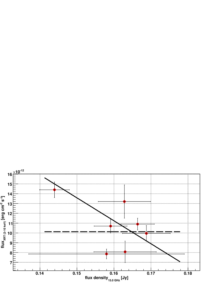
Figure 13: Integral flux measured by Swift XRT from 2 – 10 keV versus the flux density measured by OVRO for data pairs with a time difference of $<0.9$ days. A constant fit is represented by the dashed line, the solid line shows the result of a linear fit.

Since the MAGIC light curve points are only marginally significant, the feasibility of investigating correlations with other bands is limited. It should however be noted that the daily flux point with the highest significance in the MAGIC light curve appeared only $\sim$ two days after the highest Swift XRT flux had been detected. Since this high X-ray flux was accompanied by a strong hardening of the spectral index, this can be interpreted as an injection of fresh electrons into the emission region, which should cause a higher flux also at gamma-ray energies.

Considering time scales beyond the duration of this MW campaign, flux (density) changes in the radio, optical and X-ray regime were clearly detected for 1ES 2344$+$514, as can be seen from the first four light curves in Fig. 14. A fit with a constant results in $\chi^{2}\mathrm{/d.o.f.}=3929.6/317$ for OVRO, $\chi^{2}\mathrm{/d.o.f.}=2058.3/437$ for KVA and $\chi^{2}\mathrm{/d.o.f.}=491.8/66$ for Swift XRT. Also the distribution histograms of flux (density) over error (Fig. 19) show a clear deviation from a Gaussian function, where the latter would be expected for uniformly sampled light curves dominated by statistical fluctuations. The strong flare measured by XRT around MJD 54442.2 cannot be unambiguously identified in the Effelsberg or KVA light curves. In the KVA light curve, a slightly higher flux was seen $\sim$ 5.3 days after the large flare and $\sim$ 5.7 days after a smaller XRT flare (MJD 54466.5), suggestive of a time lag of the optical emission with respect to the X-rays. Also the Effelsberg measurements revealed two significant peaks (at different frequencies, though) in that time period ($\sim$ MJDs 54486 and 54547). But on a significant correlation of these high states with the XRT flares can only be speculated due to the incomplete sampling of the Swift XRT, KVA and Effelsberg light curves.

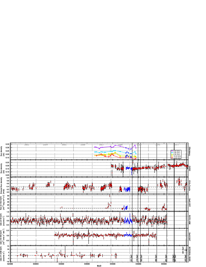
Figure 14: Long term light curves of 1ES 2344$+$514 measured by Effelsberg, OVRO, KVA$+$Tuorla, Swift XRT, RXTE ASM, Swift BAT and INTEGRAL ISGRI. The first four panels show an observation-wise binning ($<1$ day), the last three panels have been re-binned to weekly scales. The blue points mark the MJD range shown in Fig. 5. The lines in the top panel do not result from a fit but simply connect the data points. Horizontal short-dashed lines give fits with a constant. The black solid vertical lines denote the arrival time of LAT events $>100$ GeV. The ASM light curve has been cut at 01/01/2011. For clarity, two points of the BAT light curve are not shown (MJD 54177.5, rate $\left(2.26\pm 0.91\right)\cdot 10^{-3}\,\mathrm{cnts}\,\mathrm{s}^{-1}$ per detector; MJD 54541.5, rate $\left(3.16\pm 1.82\right)\cdot 10^{-3}\,\mathrm{cnts}\,\mathrm{s}^{-1}$ per detector) and the (linear) error bar of one point (MJD 53729.5) has been cut at the plot edge. Distribution histograms of the light curve points over their respective errors are given in Fig. 19. See text for details.

On time scales of years, the good sampling allows us to perform a search for correlations between the OVRO and KVA data. In order to exclude a bias of the result caused by measurement noise, OVRO data with an error $>0.02$ Jy ($\sim$ 15 % of the data) were excluded from this analysis. Using the discrete correlation function (DCF) as defined in Edelson & Krolik (1988), we searched for possible correlations for lags up to $\pm 100$ days between both data sets. Two such searches were performed, one in which the raw light curves were used, and one in which we searched for correlations after first subtracting off a low-pass filtered version of the data in order to remove long-term trends which might influence the calculation of the DCF. The analysis did not yield a significant correlation.

Investigating the light curves of RXTE ASM, Swift BAT and INTEGRAL ISGRI on time scales of one day, some outliers become apparent. These are expected from a statistical point of view, and all data points but one do not have a signal/error significantly offset from their corresponding Gaussian distribution (see Fig. 20). This point, having a signal to noise ratio of $\sim$ 5, was measured by ASM at MJD 54468.0, 1.5 days after an increased flux seen by Swift XRT and $\sim$ 3.8 days before the higher KVA state (see above). If real, it indicates that XRT detected the onset of a flare potentially even higher than the large one around MJD 54442.2, which preceded a small flare in the R-band by $\sim$ 3 – 4 days. The sparse sampling does not allow to draw further conclusions on the nature or origin of the flare.

A fit with a constant to the daily light curves is ruled out on high statistical basis for ASM and BAT ($\chi^{2}\mathrm{/d.o.f.}=4215.6/3007$ and 2364.1/1733, respectively), though not for ISGRI ($\chi^{2}\mathrm{/d.o.f.}=228.8/214$). The Gaussian fits to the signal/error distributions reveal a significant shift of the mean value to positive values for BAT and ISGRI, but not for ASM ($0.18\pm 0.03$, $0.11\pm 0.07$ and $-\left(0.07\pm 0.02\right)$ for BAT, ISGRI and ASM, respectively). Note, however, that a Gaussian statistical behaviour is not expected for ASM due to coded mask observations. In the case of BAT, Gaussian statistics is still applicable despite applying the coded mask technique due to the large number of individual detector elements. Consequently, the BAT light curve indicates significant variability of the source at hard X-rays.

The large flare detected by XRT on MJD 54442.2 is not clearly visible in the daily ASM or BAT light curve; ISGRI did not observe at that time. 1ES 2344$+$514 seems to be too faint at X-rays to be detected on daily time scales by these two instruments. Therefore, the light curves of ASM, BAT and ISGRI have been re-binned in the same way as the simultaneous BAT data (see Sect. 2.4). As an example, the weekly results are shown in Figs. 14 and 19. From the signal/error distribution histograms, no significant flares outside the Gaussian distribution are apparent for any binning and instrument except for the 1-week BAT point at MJD 54772.5 already discussed in Sect. 3.3. The large XRT flare at MJD 54442.2 is still not clearly present in any of the light curves for any binning.

The trend of a positive Gaussian mean increases with larger time bins for BAT, finally leading to the detection of 1ES 2344$+$514 as reported in the 58-Month Catalog. The light curves of ASM and BAT are not consistent with a constant flux up to quarterly binning, though the corresponding probabilities are rising with increasing time bin size. For a yearly binning, a fit with a constant yields $\chi^{2}\mathrm{/d.o.f.}=14.9/7$, $\chi^{2}\mathrm{/d.o.f.}=5.1/5$ and $\chi^{2}\mathrm{/d.o.f.}=8.2/5$ for ASM, BAT and ISGRI, respectively.

The arrival times of the nine photons with energy $>100$ GeV detected by Fermi-LAT within the first 44 months are also shown in Fig. 14. No exceptional behaviour is visible in the light curves of the other energy bands at these times.

At the time of the Metsähovi flare (MJD 55039, see Sect. 3.5.1), optical R-band monitoring data are also available. 1ES 2344$+$514 was densely covered between MJDs 54994 and 55088 with detections on daily basis from seven days before the Metsähovi flare until three days after. The best, though still insignificant, hint of a higher flux density in that period is given at MJDs 55040 and 55041. Either there was no correlation present between the R-band and 37 GHz during this flare (as the missing long-term OVRO – KVA correlation is also suggesting), or the optical monitoring missed it. A missing correlation would hint on different flaring mechanisms or, more likely, spatially separated emission regions. In the latter case, a time delay between the radio and optical emission would be expected, which may be more firmly determined based on continuous monitoring in the future. Quite interestingly, two of the Fermi-LAT events with energies $>100$ GeV were detected 46 days before and $<2$ days after the Metsähovi flare, respectively (see Table 2). On a correlation can only be speculated though, taking into account that the exact time of the flare maximum can be determined neither from the Metsähovi nor the OVRO or KVA monitoring data. Moreover, the timing of the events may be purely coincidental.

In general, the present monitoring programs at various wavelengths represent a major progress towards the understanding of blazar phenomena. Nevertheless, more efforts seem necessary, increasing the sampling density and time basis, and especially extending the monitored energy range to the X-ray and VHE regime.

4.2 Spectral Energy Distribution Modelling

4.2.1 Simultaneity

Since the gamma-ray detections were only marginally significant, (quasi-)simultaneous data sets for constructing SEDs are composed according to the X-ray flux state. We define a “low” and “high” X-ray flux SED, choosing MJDs 54760.9 (high) and 54768.8 (low). The exact observation times of the different instruments around these data sets are given in Table 4.

Table 4: Observing intervals of the SED data sets.

Data Set	Instrument	Observation Time
		[MJD]
1ES 2344$+$514 low	Effelsberg	54778.947 – 54778.950
	OVRO	54769.077
	Swift	54768.806 – 54768.948
	AGILE	54770.500 – 54800.500
	Fermi-LAT	54759.941 – 54800.897
	MAGIC	54759.941 – 54800.897
1ES 2344$+$514 high	Effelsberg	54756.960 – 54756.970
	OVRO	54761.095
	VLBA	54761.960 – 54762.42
	KVA	54761.718
	Swift	54760.899 – 54760.983
	AGILE	54770.500 – 54800.500
	Fermi-LAT	54759.941 – 54800.897
	MAGIC	54759.941 – 54800.897

The two data sets are too close in time to derive individual gamma-ray results. The corresponding ULs of AGILE-GRID and Fermi-LAT as well as the MAGIC spectrum were averaged over the entire respective observation periods and used for the modelling of both SEDs. Note that no significant variability could be found in any gamma-ray band (see Sects. 3.1,3.2), the detection of which would exclude averaging the measurements.

The 66-month BAT spectrum can be regarded as a measure of the average low flux of the source, since no significant flares are present in the BAT light curve from daily to yearly scales apart from the artificially high weekly flux point at MJD 54772.5. Taking into account that the low and high state XRT spectra have been measured in a slightly lower and higher flux state than the long-term average (judging from Fig. 14), respectively, the BAT spectrum may be considered as being quasi-simultaneous to these spectra.

The variability time scale during the observations in the radio regime is hard to assess and differs from band to band, but in general large changes in flux are not expected on time scales of $\sim$ two weeks. Therefore, some radio measurements have been included on a quasi-simultaneous basis.

For the chosen low and high state dates of 1ES 2344$+$514, there were no simultaneous measurements by KVA. For the high state, the result from the following night is used. Taking into account that the KVA measurements do not show a hint of variability throughout more than three months of observations, this procedure seems justified. On the other hand it should be noted that the simultaneous optical – X-ray data pairs are very few and especially missing for high X-ray fluxes, hence a higher optical flux during the XRT flare cannot be excluded.

4.2.2 Model Description

Two different leptonic SSC emission models have been applied to the such defined quasi-simultaneous SEDs. The one-zone model by Maraschi & Tavecchio (2003) describes the SED completely by nine parameters: the radius $R$, Doppler factor $\delta$ and magnetic field $B$ of the emission region, which contains an electron distribution following a broken power law with index $n_{1}$ for $\gamma_{\mathrm{min}}<\gamma<\gamma_{\mathrm{break}}$ and index $n_{2}$ for $\gamma_{\mathrm{break}}<\gamma<\gamma_{\mathrm{max}}$ with density $K$ at Lorentz factor $\gamma=1$. $\gamma_{\mathrm{min}}$ has been fixed to values of 1 and 4000, which represent the extreme cases of the lowest and a very high realisation, visualising a large part of the reasonable parameter range.

In the second model (Weidinger & Spanier 2010), an electron distribution with density $K$ at $\gamma_{\mathrm{min}}$ is being accelerated in a zone with radius $R_{\mathrm{acc}}$. The electrons are finally escaping the acceleration region and enter a second region, i.e. the emission region, with radius $R_{\mathrm{em}}$ where no further acceleration takes place. The magnetic field $B$ and Doppler factor $\delta$ are the same for the two regions. The resulting electron distribution as well as the spectral indices are derived self-consistently from the acceleration and cooling processes and are not determined a priori.

4.2.3 Results

The 1ES 2344$+$514 SEDs compiled from this campaign are shown in Fig. 15. The given simultaneous KVA and UVOT data have been host-galaxy corrected where necessary as well as de-reddened. Due to the strong host galaxy and the large uncertainty in its flux, the V-, B- and U-band fluxes cannot be determined with sufficient significance and hence are not shown. Since the optical data given at ASDC are not host-galaxy corrected, they have been omitted. The simultaneous XRT data were corrected for Galactic absorption. MAGIC and Whipple data were EBL de-absorbed using the model from Kneiske & Dole (2010), the archival VERITAS data by the Franceschini et al. (2008) model. The AGILE UL denotes the flux $>100$ MeV, the Fermi-LAT 1FGL ULs are given between 0.1 and 0.3 as well as 0.3 and 1 GeV. Note that the Metsähovi UL has a c.l. of 4 $\sigma$ and the IRAM ones 3 $\sigma$.

A comparison of our results to archival SED data reveals that the source has been measured in one of the lowest flux states ever obtained from X-ray to VHE gamma rays. At optical and radio frequencies, the fluxes were at a modest level.

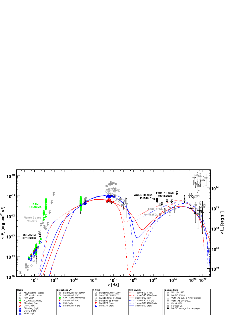
Figure 15: Simultaneous SEDs of 1ES 2344$+$514 as derived from this campaign (black, blue and red markers) together with monitoring results from F-GAMMA and the Tuorla Blazar Monitoring Program (green points) as well as archival data (shown in grey). The black MAGIC data points represent the overall flux during the campaign. “low” and “high” denote the simultaneous data sets as given in Table 4. For the one-zone model, the number given in the legend represents the value of $\gamma_{\mathrm{min}}$. See text for further details. Archival data have been taken from the ASDC SED Builder (http://tools.asdc.asi.it), Acciari et al. (2011b), Schroedter et al. (2005) (Whipple) and Albert et al. (2007b) (MAGIC). The Planck ULs were taken from Giommi et al. (2012).

For comparison, we also include published Fermi-LAT 1FGL points on a quasi-simultaneous basis, taking into account that no significant variability is present also in 2FGL. Though all points are consistent with a simple power law distribution, there seems to have been a small jump between the LAT points at 6 and 60 GeV which is hard to describe with the applied models. Either the 6 GeV point is rather low in flux or the 60 GeV point comparably high. The latter point connects rather smoothly to the MAGIC spectrum from 2005 – 6 and the VERITAS points from 2008, whereas putting more weight on the 6 GeV point the MAGIC spectrum from this campaign seems to match better the quasi-simultaneous LAT data. Since the highest energy point is subject to a rather large statistical uncertainty ($<10$ and $<20$ events in 1FGL and 2FGL, respectively) and hence prone to potential short-term flux variations, our modelling is focusing on the 0.6 – 6 GeV points. In this context, the inconsistency of the Fermi-LAT spectrum with the VHE points reported in Abdo et al. (2009b) is no longer evident using the MAGIC points from this campaign, indicating that the VHE results derived here are more representative of the average flux state of 1ES 2344$+$514.

The 66-month BAT spectrum is an adequate extrapolation of the XRT high state from this campaign. The low state spectrum, on the other hand, would require an increase of flux with rising energy, which cannot be described with the SSC models applied here. Therefore, the BAT spectrum has been considered for the fit to the high state data set only.

Note that SSC models are in general not suited to describe the low frequency (i.e. radio) emission. Photons of these energies are self-absorbed in the radiation field of the SSC emission region. The observed flux in the radio regime is probably produced by cooled electrons from an outer region of the jet which are unimportant for the modelling of the higher frequencies (Maraschi & Tavecchio 2003).

Taking this into account, both models are in reasonable agreement with the simultaneous data of 1ES 2344$+$514. The quasi-simultaneous 1FGL points disfavour the one-zone model fits having a $\gamma_{\mathrm{min}}=1$. Clearly the fits described by $\gamma_{\mathrm{min}}=4000$ are preferred, or in general values being closer to 4000. However, also for the one-zone fits with high $\gamma_{\mathrm{min}}$, a softer spectral index in the HE regime would improve the compatibility with the 1FGL data.

The derived model parameters (see Table 5) are in good agreement with typical values for HBLs. Only $\gamma_{\mathrm{min}}$ seems rather high for the one-zone model, as does $\gamma_{\mathrm{max}}$ for the low state two-zone model. Considering the exceptional faintness of 1ES 2344$+$514 across several energy bands, this concordance is not necessarily expected. Consequently, either the low flux state detected in this campaign does (still) not represent the “quiescent” state of the source, or the quiescent state model parameters do not differ considerably from the already known ones. The ULs on size and magnetic field strength in the dominating radio emitting region derived from VLBA observations (Sokolovsky et al. 2010a) do not contradict the parameters of the blazar emission zone as given in Table 5.

Table 5: Model parameters. See text or reference for an explanation of the models. The used data sets and their simultaneity are discussed in the text.

Reference	This Campaign				Albert et al. (2007b)		Tavecchio et al. (2010)	Acciari et al. (2011b)
Model Reference	(1)		(2)		(3)		(1)	(3)
Flux Level	low	high	low	high	low	high	…	low	high
$B$ [G]	0.07		0.05	0.09	0.10	0.08	0.1	0.09	0.03
$\delta$	20		26	29	8	15	25	13	20
$R_{\mathrm{em}}$ [$10^{15}$ cm]	3	4	9	5	10		4	10
$R_{\mathrm{acc}}$ [$10^{13}$ cm]	…	…	8	13	…	…	…	…	…
$K$ [$10^{5}\,\mathrm{cm}^{-3}$]	4.5	1.9	0.2	0.1	$\sim$ 0.5	$\sim$ 0.4	0.3	$\sim$ 0.4
$e_{1}$	2.3		2.5	2.3	2.2		2	2.5	2.3
$e_{2}$	3.4	3.2	3.5	3.3	3.2		3.2	3.2
$\gamma_{\mathrm{min}}$	1 or 4000		1800	550	$\sim$ 2500	$\sim$ 1500	1 (8000)	$\sim$ 200
$\gamma_{\mathrm{break}}$ [$10^{4}$]	5	8	10	3	$\sim$ 15		1	$\sim$ 40	$\sim$ 50
$\gamma_{\mathrm{max}}$ [$10^{6}$]	0.7	1.5	6.3	1.5	$\sim$ 0.8	$\sim$ 1.6	0.7	$\sim$ 2.0

Comparing the high and low state in terms of the one-zone model, the latter is explained by a softer electron spectral index as well as a lower $\gamma_{\mathrm{break}}$ and $\gamma_{\mathrm{max}}$. In the case of the two-zone model, the magnetic field drops consistently accompanied by a higher $\gamma_{\mathrm{min}}$, $\gamma_{\mathrm{break}}$ and $\gamma_{\mathrm{max}}$. The parameter changes of each model are best explained by a change in the acceleration properties of the non-thermal electrons, i.e. the efficiency of the underlying Fermi processes drops or rises respectively (we recall that $\gamma_{\mathrm{break}}$ is not computed self-consistently in case of the one-zone model). This behaviour may be caused by the emitting volume leaving a standing feature along the jet (see e.g. Marscher et al. 2008) or, more likely, due to the observation of two independent blobs.

It is interesting to note that the luminosity of the inverse Compton component of the low (i.e. low X-ray flux) state SED exceeds the one of the high state SED for all applied models. Specifically in the case of the one-zone model, this makes the bolometric luminosities $L_{\mathrm{bol}}$ of the two flux states comparable. For $\gamma_{\mathrm{min}}=1$ (4000), $L_{\mathrm{bol,low}}=10^{44.7}$ ($10^{44.6}$) and $L_{\mathrm{bol,high}}=10^{44.8}$ ($10^{44.7}$) erg s^-1, which is basically identical considering the uncertainties involved.

Due to the differences between the two model approaches at sub-optical frequencies and in the hard X-ray to soft gamma-ray band, it is in principle possible to distinguish between the validity of the models. The first frequency band is covered by Planck, though no detection of the source has been reported in The Early Release Compact Source Catalogue (Ade et al. 2011), containing the results of the first ten months of operation. Swift BAT, INTEGRAL IBIS as well as AGILE-GRID and Fermi-LAT cover the second window, but are not sensitive enough to detect the source during low flux states on short time scales. To exclude one of these models, a more sensitive instrumentation than currently available is needed.

Within this campaign, a small shift between the synchrotron peak in the high and low state may be present (see Fig. 15). A peak estimate from the data has been obtained by fitting the optical and X-ray SED points by a parabolic power-law in apex form (see e.g. Tramacere et al. 2007):

$$\nu F_{\nu}=f_{0}\cdot 10^{-b\cdot\left(\log_{10}\left(\nu/\nu_{\mathrm{peak}}\right)\right)^{2}}\,\mathrm{erg}\,\mathrm{cm}^{-2}\,\mathrm{s}^{-1}$$ (2)

where $\nu_{\mathrm{peak}}$ is the frequency of the synchrotron peak. The result is shown in Fig. 16. From the fit to the low state data ($\chi^{2}\mathrm{/d.o.f.}=6.5/8$), the peak energy is determined marginally significant as $\left(0.27\pm 0.24\right)$ keV. In the high state case, the goodness of fit is higher ($\chi^{2}\mathrm{/d.o.f.}=5.6/10$), but the fit fails to determine the peak energy ($\left(2.8\pm 4.5\right)$ keV). Additionally, a parabolic power law is not clearly preferred over a simple power law in both cases (logarithmic likelihood ratio of 79.5 % and 95.7 % for the low and high state, respectively). Consequently the data are insufficient to directly constrain changes of the peak energy. As determined from the one-zone $\gamma_{\mathrm{min}}=4000$ (two-zone) modelling, the peak shifted from $\sim$ 0.15 keV to $\sim$ 1.7 keV ($\sim$ 0.13 keV to $\sim$ 0.46 keV) between the low and high flux state. All these values are far from the extreme blazar characteristics 1ES 2344$+$514 has shown during high X-ray flux states, which is expected due to the rather small flux difference between the two states observed here.

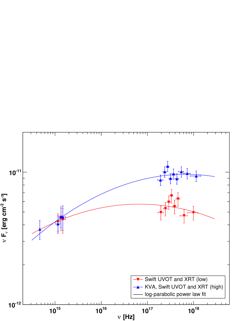
Figure 16: Simultaneous KVA, Swift UVOT and Swift XRT data from the low (red downward triangles) and high (blue upward triangles) state. The solid lines describe a fit with a log-parabolic power law as stated in Eq. 2. R-band and UV data have been de-reddened, the former additionally host galaxy corrected. X-ray data have been corrected for Galactic absorption.

4.3 Comparison with Archival Campaigns

We compare the model parameters obtained from this campaign with three other previous MW data sets reported for 1ES 2344$+$514. The parameters are listed in Table 5.

4.3.1 Archival Campaign Description

In Albert et al. (2007b), a homogeneous one-zone SSC model (Krawczynski et al. 2004) was applied to both a low and high state of the source. The low state data consisted of simultaneous measurements of MAGIC, KVA and an ASM UL taken between 08/2005 and 01/2006, where BeppoSAX data taken 06/1998 were added as a low state X-ray spectral template. Data by BeppoSAX and a simultaneous UL by Whipple were combined with an archival Whipple high state spectrum to describe the high state. Consequently the simultaneous data set was not very constraining and the SED models rather speculative, as noted by the authors.

Tavecchio et al. (2010) were using the results from the first three months of Fermi-LAT observations and combined them with archival, non-contemporaneous data of 1ES 2344$+$514 from the radio up to the VHE band. They used the one-zone SSC model also applied in this work.

A more recent campaign, also using the model of Krawczynski et al. (2004), combined measurements by VERITAS, RXTE PCA, Swift XRT and Swift UVOT from 10/2007 until 01/2008 (Acciari et al. 2011b). The low state SED was modelled using the time-averaged VERITAS measurements (excluding a large flare) and a representative moderate X-ray flux 1-day spectrum by XRT and PCA, similar to the procedure used in this campaign for the low state SED. Note however that the MAGIC light curve from this campaign did not show significant variability, opposite to the VERITAS measurements even after the exclusion of the flare ($F_{\mathrm{var}}=\left(34\pm 16\right)$ %). The high state SED data set was built from the highest fluxes measured by VERITAS and Swift XRT together with the corresponding UVOT data. Though the gamma-ray and X-ray flares seem to have been correlated, they were separated by $>24$ hours. Note that the flux doubling time scale of the VHE and X-ray flare was also $\sim$ 24 hours, thus the true simultaneous fluxes could have been different by a factor of $\sim$ 2. The model predicted significantly higher, in the high state by $\sim$ one order of magnitude, fluxes than the 1FGL points. Since these were taken after the MW campaign, higher fluxes in the LAT range during the observations indeed cannot be excluded, despite the rather constant emission of the source for two years since the launch of Fermi.

4.3.2 Model Parameter Comparison

While the model parameters are in general interdependent and hence difficult to compare, we can more easily investigate general trends. Note that the models shown in Albert et al. (2007b) and Tavecchio et al. (2010) were not constrained by simultaneous measurements as well as partly affected by incorrectly adopted data (see footnotes 19 and 20), thus the results have to be taken with care. All models indicate a rather weak magnetic field and high Doppler factor, similar to values typically found for HBLs (see e.g. Tavecchio et al. 2010). Variability is not explained in a unique way. For instance, changes in $B$ and $\delta$ can occur, but do not have to. Variability mostly arises by changes in the electron distributions, i.e. different spectral indices or energy distributions. Particularly in the case of this campaign, the spectral indices are harder in the high flux state. It is interesting to note that the size of the emission region is often not changing between the different flux states presented in Table 5. That can be explained within the standing shock scenario, where variability would be caused by structural changes due to variations of the flow (Tagliaferri et al. 2008). However, this behaviour is not expected if the two states correspond to the emission of one moving and expanding blob of electrons within the jet (e.g. Atoyan & Aharonian 1999; Sikora et al. 2001) at two different times. This argument does not apply in the case of Albert et al. (2007b) though since the presented low and high state are not causally connected but artificially constructed. For Acciari et al. (2011b), another flare occurred between the high and low state SEDs, giving evidence that there is no causal connection. Moreover, the time differences between the two flux states are, also in the case of this campaign, too long to allow both to be caused by the same emitting region, at least if the emission region is visualised as a travelling and expanding (with $v_{\mathrm{exp}}$ $\sim$ $c$) blob (which would expand by several orders of magnitudes within one week). To allow for a causal connection between the high and low state, the emission region has to be externally confined in some way (e.g. by magnetic fields).

In general, the parameters found in this campaign are in good agreement with archival values. It should however be noted that the range for some parameters is rather broad, due to the inter-dependencies of the parameters and non-unique solutions of the model fits. More data and more MW campaigns in different flux states are needed to fully constrain the models and reduce the allowed parameter ranges.

5 Summary and Conclusions

In this paper, the results from the first MW campaign on 1ES 2344$+$514 from the radio to the TeV band have been presented and discussed, also taking into account multi-band long-term data. The MW observations took place from 10/2008 until 01/2009, where the $\sim$ 40 day long core campaign was conducted in October and November. The source was found at low to modest flux states at radio and optical frequencies, whereas at X-rays and gamma rays, the flux level was amongst the lowest ever reported for 1ES 2344$+$514. Due to this faintness, HE observations did not result in a detection during the campaign, and the time-averaged VHE detection was only marginally significant. Nevertheless we were able to obtain a reliable VHE spectrum due to the long observation time of $\sim$ 20 hours, the good event statistics and the source being a well-known VHE emitter.

The VHE analysis suggested a rather hard spectral index, which, if real, would be opposite to the “harder when brighter” trend found in general for HBLs. The flux was consistent with constant during the campaign. At X-rays, a moderate flare was detected with $\sim$ halving of the flux within several days. During the flare, hints for a counter-clockwise behaviour in the hardness ratio – integral flux plane were found, indicating that the flare was caused by a shock front characterised by comparable cooling and acceleration time scales. This finding was strengthened by the constant spectral index during the flare. Taking into account all X-ray observations during the campaign, the spectral index still did not show significant variability, though a potential correlation between the X-ray index and the X-ray integral flux was visible. The evolution of the hardness ratio with the integral flux corroborated that “harder when brighter” trend, confirming findings reported in the literature for 1ES 2344$+$514. No significant variability could be found at optical and UV frequencies. From VLBA observations, the size of the radio core could be determined or constrained at several frequencies, yielding values of the order of 10¹⁷ cm. This is more than one order of magnitude above the size determined from SED modelling, indicating a different origin of the radio and SSC emission.

1ES 2344$+$514 exhibited significant variability only at low frequency radio and X-ray bands during the campaign. Due to that as well as unfortunate sampling and technical problems, the basis for cross-band correlations for the time of the MW campaign is too short for a meaningful investigation. For a flare observed at the end of the core campaign, indications were found suggesting it may have been caused by injection of fresh electrons into the jet.

On time scales longer than this campaign, significant variability was evident for the radio, optical and X-ray regimes whereas the high energy gamma-ray light curve from 2FGL was consistent with being constant. In contrast to the low and constant emission found by Fermi-LAT, the events with energies above 100 GeV detected from 1ES 2344$+$514 indicate that the source may have a comparably high flaring duty cycle.

Different feature characteristics were found in the Effelsberg light curve at low radio frequencies, indicating a possible re-acceleration of particles within the jet. The difference between these features may be explained by changes in the environment of the particles. The behaviour of the combined long-term radio spectra of the source gave rise to interpreting the emission as a two-component system composed of quiescent diffuse emission overlaid by frequent outbursts. The signature of such shocks should be traceable from higher to lower radio frequencies. One flaring event at 37 GHz was visible on the investigated time scales, but the expected signatures could not be found in the other radio bands. The OVRO measurements had some gaps during these days but did not show evidence of a significant flux increase. Two of the nine photons with an energy $>100$ GeV were detected by Fermi-LAT around the time of that flare. A counterpart of this event was not found in the optical R-band despite rather good optical coverage, which would hint at a different emission region of the 37 GHz and R-band emission if not due to sampling effects. The flare on its own represents a rare event for HBLs concerning its amplitude and time scale. A long-term correlation analysis between the 15.0 GHz and R-band was conducted, yielding no significant correlation between the two bands.

The observed flat parsec-scale radio spectrum together with the frequency-dependent core size (Table 3) and position shift, indicated by a comparison of core–jet component distances measured at 15.4 and 43.2 GHz by Piner & Edwards (2004) and Piner et al. (2010), can be interpreted as a signature of a Blandford & Königl (1979) type jet. Analysing all MOJAVE observations conducted until today, no significant motion of the three identified jet components on time scales of eleven years could be found, opposite to claims in previous publications. The apparent jet speeds of the components were $\beta_{\mathrm{app}}<0.13$, with the most constraining value having been $-0.01\pm 0.02$.

Monitoring at soft and hard X-rays revealed only one significant individual detection, though a general trend of positive flux for BAT and ISGRI was apparent, leading to the detection of the source by BAT from 58 months of data. The individual detection, found by ASM, was coincident within a few days with a higher state seen by XRT and a hint for an R-band flare seen by KVA. Also the Effelsberg measurements showed increased activity around this time period. However the sampling was insufficient for a meaningful investigation of the origin of the flare. The BAT light curve was significantly variable. The long-term trend measured by ASM did not show a hint of a positive signal.

From the observations, (quasi-)simultaneous SEDs for a low and high X-ray flux state were constructed and modelled using a one-zone SSC as well as a self-consistent two-zone SSC model. Both could describe the data well, however quasi-simultaneous HE data posed some challenges for the modelling. In particular, these disfavoured the one-zone models having a $\gamma_{\mathrm{min}}$ of unity, being in general better described by the upper part of the tested parameter range. The one- and two-zone models suggested a shift of the first SED peak by $\sim$ 1.1 and $\sim$ 0.4 orders of magnitude, respectively. Direct fitting of the combined optical and X-ray data did not result in a firm determination of the peak energies. The individual parameters retrieved from the one- and two-zone modelling were mostly in agreement between these two different model approaches for each of the two flux states. They were consistent with values found in archival campaigns as well as standard parameter ranges for HBLs. This concordance is not self-evident in the context of “quiescent” state emission, where the quiescent spectrum should be dominated by a low and constant flux component which possibly has different spectral characteristics. Either the “quiescent” state was not detected within this MW campaign, or the corresponding model parameters do not differ significantly from the typical values. The two applied models showed significant differences at high radio frequencies and in the hard X-ray to HE bands. In the future, instruments more sensitive in these regimes could probe the validity of the models.

Appendix A Detailed Results

Simple Power Law Fit Log-Parabolic Power Law Fit Obs. ID MJD_start Exp. $F\left(2-10\,\mathrm{keV}\right)$ $a$ $\chi^{2}_{\mathrm{red}}\mathrm{/d.o.f.}$ $F\left(0.2-1\,\mathrm{keV}\right)$ $F\left(2-10\,\mathrm{keV}\right)$ $a$ $b$ $\chi^{2}_{\mathrm{red}}\mathrm{/d.o.f.}$ L HR [ks] [$10^{-12}\,\mathrm{erg}\,\mathrm{cm}^{-2}\,\mathrm{s}^{-1}$] [$10^{-12}\,\mathrm{erg}\,\mathrm{cm}^{-2}\,\mathrm{s}^{-1}$] [$10^{-12}\,\mathrm{erg}\,\mathrm{cm}^{-2}\,\mathrm{s}^{-1}$] [%] 35031019 54730.158 0.59 … … … … … … … … … … 35031021 54745.554 1.75 10.8 $\pm$ 0.9 2.03 $\pm$ 0.11 0.77/17 2.50 $\pm$ 0.30 9.2 $\pm$ 0.8 1.79 $\pm$ 0.25 0.51 $\pm$ 0.30 0.61/18 85.1 $1.17\pm 0.12$ 35031022 54749.513 0.94 9.8 $\pm$ 1.4 2.12 $\pm$ 0.23 0.79/7 3.05 $\pm$ 0.50 9.8 $\pm$ 1.5 2.12 $\pm$ 0.35 0.00 $\pm$ 0.00 0.93/6 0.0 $0.80\pm 0.12$ 35031023 54757.762 1.23 9.5 $\pm$ 1.1 2.14 $\pm$ 0.18 1.55/13 3.09 $\pm$ 0.50 9.5 $\pm$ 1.4 2.14 $\pm$ 0.30 0.00 $\pm$ 0.00 1.68/12 0.0 $0.95\pm 0.13$ 35031024 54759.895 2.23 14.2 $\pm$ 0.9 1.94 $\pm$ 0.09 1.10/30 2.90 $\pm$ 0.25 13.0 $\pm$ 0.8 1.80 $\pm$ 0.18 0.27 $\pm$ 0.25 1.07/29 82.9 $1.21\pm 0.10$ 35031025 54760.899 2.31 14.4 $\pm$ 0.8 1.98 $\pm$ 0.08 1.04/42 3.16 $\pm$ 0.22 13.0 $\pm$ 0.9 1.80 $\pm$ 0.16 0.36 $\pm$ 0.26 0.95/41 96.0 $1.17\pm 0.09$ 35031026 54761.904 2.27 13.4 $\pm$ 0.7 1.97 $\pm$ 0.08 1.32/32 2.91 $\pm$ 0.23 12.3 $\pm$ 0.9 1.84 $\pm$ 0.17 0.26 $\pm$ 0.25 1.29/31 85.6 $1.22\pm 0.10$ 35031027 54762.908 2.42 10.9 $\pm$ 0.6 2.02 $\pm$ 0.09 1.12/28 1.67 $\pm$ 0.22 10.3 $\pm$ 0.8 1.94 $\pm$ 0.16 0.17 $\pm$ 0.17 1.12/27 69.9 $1.06\pm 0.09$ 35031028 54763.167 4.91 10.5 $\pm$ 0.6 2.03 $\pm$ 0.06 1.20/48 2.61 $\pm$ 0.17 9.7 $\pm$ 0.6 1.92 $\pm$ 0.12 0.25 $\pm$ 0.21 1.15/47 93.0 $1.07\pm 0.07$ 35031029 54764.857 1.58 10.0 $\pm$ 0.8 2.09 $\pm$ 0.12 0.97/17 2.64 $\pm$ 0.30 9.0 $\pm$ 1.0 1.92 $\pm$ 0.27 0.35 $\pm$ 0.34 0.93/16 78.5 $1.09\pm 0.12$ 35031030 54765.917 2.53 9.6 $\pm$ 0.7 2.01 $\pm$ 0.08 1.36/26 2.11 $\pm$ 0.23 8.4 $\pm$ 0.8 1.75 $\pm$ 0.19 0.51 $\pm$ 0.30 1.07/25 98.6 $1.13\pm 0.10$ 35031031 54766.865 1.19 8.1 $\pm$ 1.1 2.10 $\pm$ 0.20 0.88/8 2.25 $\pm$ 0.50 7.2 $\pm$ 1.2 1.99 $\pm$ 0.40 0.26 $\pm$ 0.26 0.99/7 24.9 $0.86\pm 0.13$ 35031032 54767.869 2.75 8.0 $\pm$ 0.6 2.15 $\pm$ 0.10 0.76/26 2.58 $\pm$ 0.25 8.0 $\pm$ 0.9 2.14 $\pm$ 0.13 0.00 $\pm$ 0.00 0.79/25 6.9 $0.87\pm 0.08$ 35031033 54768.806 2.29 7.9 $\pm$ 0.5 2.04 $\pm$ 0.11 0.99/18 1.82 $\pm$ 0.20 6.9 $\pm$ 0.8 1.78 $\pm$ 0.26 0.51 $\pm$ 0.42 0.84/17 92.9 $1.13\pm 0.12$ 35031034 54769.932 1.87 11.5 $\pm$ 0.7 1.96 $\pm$ 0.10 1.09/20 2.44 $\pm$ 0.25 10.7 $\pm$ 0.9 1.83 $\pm$ 0.22 0.25 $\pm$ 0.25 1.07/19 76.4 $1.21\pm 0.12$ 35031035 54770.881 2.10 9.6 $\pm$ 0.7 2.06 $\pm$ 0.11 0.58/21 2.60 $\pm$ 0.25 9.3 $\pm$ 1.0 2.02 $\pm$ 0.20 0.00 $\pm$ 0.00 0.60/20 31.8 $1.01\pm 0.10$ 35031036 54771.933 1.65 9.9 $\pm$ 0.8 1.99 $\pm$ 0.11 1.36/15 1.93 $\pm$ 0.22 8.6 $\pm$ 0.9 1.58 $\pm$ 0.32 0.73 $\pm$ 0.50 1.01/14 97.7 $1.23\pm 0.14$ 35031037 54772.892 0.19 … … … … … … … … … … 35031038 54773.892 0.94 13.2 $\pm$ 1.7 1.86 $\pm$ 0.22 0.30/7 2.43 $\pm$ 0.50 12.4 $\pm$ 2.0 1.80 $\pm$ 0.50 0.14 $\pm$ 0.14 0.35/6 0.0 $1.17\pm 0.18$ 35031039 54777.483 1.59 10.7 $\pm$ 0.7 2.16 $\pm$ 0.12 1.36/22 3.55 $\pm$ 0.30 10.6 $\pm$ 1.2 2.15 $\pm$ 0.25 0.00 $\pm$ 0.00 1.43/19 89.2 $0.99\pm 0.10$ 35031040 54784.592 1.06 16.6 $\pm$ 1.7 1.76 $\pm$ 0.13 0.32/13 2.48 $\pm$ 0.30 15.9 $\pm$ 1.9 1.69 $\pm$ 0.30 0.13 $\pm$ 0.13 0.33/12 33.5 $1.47\pm 0.18$

Table 6: Swift XRT results.

Table 7: Analysed MAGIC data sets and results using detection cuts to determine the significance and open cuts for the integral fluxes.

Data Set	Obs. Time	$t_{\mathrm{eff}}$	$S$	$F\left(>170\,\mathrm{GeV}\right)$
	[MJD]	[h]		[$10^{-12}\,\mathrm{ph}\,\mathrm{cm}^{-2}\,\mathrm{s}^{-1}$]
all data	54780.419	20.75	3.5	$7.4\pm\phantom{0}2.1$
period 1	54763.433	10.26	1.9	$3.2\pm\phantom{0}2.9$
period 2	54793.858	10.49	3.1	$11.5\pm\phantom{0}2.9$
21 Oct.	54759.973	1.42	1.3	$10.6\pm\phantom{0}8.0$
22 Oct.	54760.960	1.41	0.6	$9.3\pm\phantom{0}7.8$
23 Oct.	54761.954	1.35	1.1	$<17.4$
24 Oct.	54762.931	1.42	0.4	$<12.5$
25 Oct.	54763.949	3.22	1.5	$<15.6$
26 Oct.	54764.946	1.14	0.0	$<19.5$
28 Oct.	54766.919	0.30	$-2.0$	$<\phantom{0}1.7$
17 Nov.	54786.862	1.03	2.5	$27.0\pm\phantom{0}9.9$
18 Nov.	54787.873	2.14	$-0.1$	$<19.7$
19 Nov.	54788.888	1.77	2.0	$16.0\pm\phantom{0}7.2$
24 Nov.	54793.866	2.12	1.2	$9.5\pm\phantom{0}6.6$
25 Nov.	54794.866	2.01	1.4	$6.5\pm\phantom{0}6.4$
28 Nov.	54797.841	0.62	$-1.1$	$<16.5$
01 Dec.	54800.879	0.81	2.0	$22.3\pm 10.0$

Table 8: Calculated HE luminosities and number of events above 100 GeV detected by Fermi-LAT from five HBLs.

Source	z	Index	$L_{\mathrm{60\,GeV}}$	$N$	$N_{\mathrm{s}}$
			[$10^{43}$ erg s-1]
Mrk 421	0.030	$1.77\pm 0.01$	$19.2\pm 1.1$	35	18
Mrk 501	0.034	$1.74\pm 0.03$	$6.95\pm 0.75$	16	10
1ES 2344$+$514	0.044	$1.72\pm 0.08$	$2.30\pm 0.56$	9	9
Mrk 180	0.046	$1.74\pm 0.08$	$2.01\pm 0.51$	1	1
1ES 1959$+$650	0.048	$1.94\pm 0.03$	$6.00\pm 0.80$	3	4

Table 9: Swift UVOT results.

Obs. ID	MJDstart	Exp.	$F_{\mathrm{V}}$	$F_{\mathrm{B}}$	$F_{\mathrm{U}}$	$F_{\mathrm{UVW1}}$	$F_{\mathrm{UVM2}}$	$F_{\mathrm{UVW2}}$
		[ks]	[mag]	[mag]	[mag]	[mag]	[mag]	[mag]
35031019	54730.158	0.89	15.45 $\pm$ 0.10	16.47 $\pm$ 0.10	16.69 $\pm$ 0.12	17.27 $\pm$ 0.20	17.76 $\pm$ 0.30	17.76 $\pm$ 0.15
35031021	54745.554	1.63	15.46 $\pm$ 0.10	16.49 $\pm$ 0.10	16.57 $\pm$ 0.12	17.20 $\pm$ 0.20	17.79 $\pm$ 0.30	17.63 $\pm$ 0.20
35031022	54749.513	0.88	15.47 $\pm$ 0.07	16.45 $\pm$ 0.07	16.53 $\pm$ 0.10	17.15 $\pm$ 0.10	17.57 $\pm$ 0.15	17.41 $\pm$ 0.10
35031023	54757.769	1.14	15.46 $\pm$ 0.10	16.52 $\pm$ 0.10	16.71 $\pm$ 0.12	17.30 $\pm$ 0.20	17.74 $\pm$ 0.30	17.49 $\pm$ 0.15
35031024	54759.895	2.18	15.47 $\pm$ 0.07	16.51 $\pm$ 0.07	16.66 $\pm$ 0.10	17.31 $\pm$ 0.10	17.73 $\pm$ 0.15	17.66 $\pm$ 0.10
35031025	54760.899	2.26	15.46 $\pm$ 0.07	16.52 $\pm$ 0.07	16.69 $\pm$ 0.10	17.27 $\pm$ 0.10	17.66 $\pm$ 0.15	17.62 $\pm$ 0.10
35031026	54761.904	2.23	15.46 $\pm$ 0.07	16.47 $\pm$ 0.07	16.56 $\pm$ 0.10	17.16 $\pm$ 0.10	17.68 $\pm$ 0.15	17.66 $\pm$ 0.10
35031027	54762.908	2.38	15.45 $\pm$ 0.07	16.46 $\pm$ 0.07	16.52 $\pm$ 0.10	17.17 $\pm$ 0.10	17.41 $\pm$ 0.15	17.54 $\pm$ 0.10
35031028	54763.167	4.83	15.46 $\pm$ 0.05	16.51 $\pm$ 0.05	16.57 $\pm$ 0.10	17.19 $\pm$ 0.10	17.59 $\pm$ 0.15	17.57 $\pm$ 0.10
35031029	54764.857	1.52	15.50 $\pm$ 0.07	16.46 $\pm$ 0.10	16.50 $\pm$ 0.10	17.10 $\pm$ 0.15	17.33 $\pm$ 0.20	17.50 $\pm$ 0.10
35031030	54765.917	2.48	15.41 $\pm$ 0.07	16.50 $\pm$ 0.07	16.57 $\pm$ 0.10	17.31 $\pm$ 0.10	17.58 $\pm$ 0.15	17.62 $\pm$ 0.10
35031031	54766.865	1.15	15.41 $\pm$ 0.10	16.49 $\pm$ 0.10	16.61 $\pm$ 0.10	17.20 $\pm$ 0.10	17.56 $\pm$ 0.30	17.55 $\pm$ 0.15
35031032	54767.869	2.68	15.48 $\pm$ 0.07	16.51 $\pm$ 0.10	16.65 $\pm$ 0.10	17.37 $\pm$ 0.10	17.80 $\pm$ 0.20	17.78 $\pm$ 0.10
35031033	54768.806	1.25	15.44 $\pm$ 0.07	16.50 $\pm$ 0.07	16.60 $\pm$ 0.10	17.23 $\pm$ 0.10	17.66 $\pm$ 0.20	17.67 $\pm$ 0.10
35031034	54769.932	1.82	15.50 $\pm$ 0.07	16.52 $\pm$ 0.07	16.67 $\pm$ 0.10	17.48 $\pm$ 0.10	17.62 $\pm$ 0.15	17.70 $\pm$ 0.10
35031035	54770.881	2.05	…	…	…	…	…	…
35031036	54771.933	1.63	15.49 $\pm$ 0.07	16.51 $\pm$ 0.07	16.73 $\pm$ 0.10	17.38 $\pm$ 0.10	17.66 $\pm$ 0.15	17.58 $\pm$ 0.10
35031037	54772.892	0.18	…	16.54 $\pm$ 0.07	16.77 $\pm$ 0.10	17.22 $\pm$ 0.10	…	…
35031038	54773.892	0.91	15.40 $\pm$ 0.07	16.44 $\pm$ 0.07	16.54 $\pm$ 0.10	17.12 $\pm$ 0.10	17.51 $\pm$ 0.20	17.49 $\pm$ 0.15
35031039	54777.483	1.54	15.39 $\pm$ 0.07	16.48 $\pm$ 0.07	16.54 $\pm$ 0.10	17.21 $\pm$ 0.10	17.62 $\pm$ 0.15	17.59 $\pm$ 0.10
35031040	54784.592	1.03	15.50 $\pm$ 0.07	16.52 $\pm$ 0.07	16.69 $\pm$ 0.10	17.36 $\pm$ 0.10	17.52 $\pm$ 0.15	17.68 $\pm$ 0.10

Table 10: Gaussian Component Properties of 1ES 2344$+$514 measured with the VLBA at 15.4 GHz.

Component	Epoch	$r$	$\theta$	$S$	Maj.	Axial	PA	log $T_{\mathrm{b}}$	$v_{\mathrm{app}}$	$\beta_{\mathrm{app}}$
		[mas]	[deg]	[mJy]	[mas]	Ratio	[deg]	[K]	[$\mu\mathrm{as\,yr^{-1}}$]
Core	1999.75	…	…	128.9	0.05	1.00	…	11.37	…	…
	1999.85	…	…	136.4	…	…	…	…
	2000.02	…	…	126.9	…	…	…	…
	2000.22	…	…	134.4	…	…	…	…
	2008.41	…	…	107.7	0.05	1.00	…	11.37
	2008.76	…	…	97.9	0.16	0.49	322	10.59
	2008.81	…	…	102.2	0.07	1.00	…	10.98
	2009.15	…	…	78.9	0.22	0.21	317	10.62
	2009.42	…	…	83.6	0.05	1.00	…	11.24
	2009.51	…	…	94.3	0.17	0.27	322	10.81
	2009.63	…	…	81.7	0.21	0.30	316	10.50
	2009.94	…	…	98.7	0.17	0.28	317	10.83
	2010.71	…	…	100.6	0.08	1.00	…	10.90
	2010.84	…	…	116.9	0.08	1.00	…	10.96
C 3	1999.75	0.543	126.1	003.2	0.20	1.00	…	8.62	$-5\pm\phantom{0}7$	$-0.01\pm 0.02$
	1999.85	0.688	129.3	003.1	…	…	…	…
	2000.02	0.774	133.6	001.8	0.13	1.00	…	8.77
	2000.22	0.491	134.6	005.2	0.31	1.00	…	8.44
	2008.41	0.401	141.8	10.1	0.30	1.00	…	8.78
	2008.76	0.630	136.6	007.7	0.22	1.00	…	8.91
	2008.81	0.516	138.2	10.8	0.19	1.00	…	9.21
	2009.15	0.728	138.3	007.4	0.20	1.00	…	8.97
	2009.42	0.446	135.5	11.6	0.15	1.00	…	9.41
	2009.51	0.591	140.4	008.3	0.14	1.00	…	9.36
	2009.63	0.665	138.8	009.4	0.32	1.00	…	8.68
	2009.94	0.637	136.8	008.0	0.20	1.00	…	9.03
	2010.71	0.535	140.2	17.0	0.34	1.00	…	8.89
	2010.84	0.554	138.4	10.7	0.16	1.00	…	9.34
C 2	1999.75	1.257	135.4	006.2	0.46	1.00	…	8.19	$\phantom{0}\phantom{-}5\pm\phantom{0}7$	$\phantom{-}0.01\pm 0.02$
	1999.85	1.538	135.9	003.6	0.13	1.00	…	9.06
	2000.02	1.558	135.3	003.2	0.29	1.00	…	8.29
	2000.22	1.541	138.6	005.0	0.44	1.00	…	8.13
	2008.41	1.422	137.7	006.5	0.55	1.00	…	8.05
	2008.76	1.731	140.5	004.9	0.43	1.00	…	8.14
	2008.81	1.448	140.6	006.4	0.43	1.00	…	8.26
	2009.15	1.521	141.1	005.0	0.40	1.00	…	8.20
	2009.42	1.416	138.8	006.9	0.56	1.00	…	8.06
	2009.51	1.394	139.5	007.2	0.55	1.00	…	8.10
	2009.63	1.590	141.4	006.7	0.73	1.00	…	7.81
	2009.94	1.491	141.3	006.9	0.50	1.00	…	8.16
	2010.71	1.657	142.3	007.7	0.66	1.00	…	7.96
	2010.84	1.481	141.5	12.9	0.75	1.00	…	8.07
C 1	1999.75	2.644	146.1	004.5	0.76	1.00	…	7.61	$\phantom{-}21\pm 24$	$\phantom{-}0.06\pm 0.07$
	1999.85	2.832	141.9	003.1	0.73	1.00	…	7.48
	2008.76	3.410	142.9	003.7	0.75	1.00	…	7.54
	2008.81	2.725	140.2	003.1	1.18	1.00	…	7.07
	2009.15	2.986	144.6	005.5	1.60	1.00	…	7.05
	2009.42	3.007	140.9	003.2	1.10	1.00	…	7.15
	2009.51	2.553	141.7	002.7	0.34	1.00	…	8.08
	2009.63*	4.495	146.8	004.5	1.80	1.00	…	6.85
	2009.94	2.998	142.3	003.3	1.44	1.00	…	6.92

Figure 19: Distribution of flux density, flux or rate divided by the error for the individual light curves shown in Fig. 14, for the last three panels including a fit with a Gaussian (shown in grey). See text for details.

Figure 20: Distribution of rate divided by the error for the individual daily-binned light curves of RXTE ASM, Swift BAT and INTEGRAL ISGRI including a fit with a Gaussian (shown in grey). See text for details.