A reproducing kernel Hilbert space approach to functional linear regression

Abstract

We study in this paper a smoothness regularization method for functional linear regression and provide a unified treatment for both the prediction and estimation problems. By developing a tool on simultaneous diagonalization of two positive definite kernels, we obtain shaper results on the minimax rates of convergence and show that smoothness regularized estimators achieve the optimal rates of convergence for both prediction and estimation under conditions weaker than those for the functional principal components based methods developed in the literature. Despite the generality of the method of regularization, we show that the procedure is easily implementable. Numerical results are obtained to illustrate the merits of the method and to demonstrate the theoretical developments.

and t1Supported in part by NSF Grant DMS-MPSA-0624841 and NSF CAREER Award DMS-0846234. t2Supported in part by NSF Grant DMS-0604954 and NSF FRG Grant DMS-0854973.

1 Introduction

Consider the following functional linear regression model where the response $Y$ is related to a square integrable random function $X(\cdot)$ through

$$Y=\alpha_{0}+\int_{\mathcal{T}}X(t)\beta_{0}(t)\,dt+\varepsilon.$$ (1)

Here $\alpha_{0}$ is the intercept, $\mathcal{T}$ is the domain of $X(\cdot)$, $\beta_{0}(\cdot)$ is an unknown slope function and $\varepsilon$ is a centered noise random variable. The domain $\mathcal{T}$ is assumed to be a compact subset of an Euclidean space. Our goal is to estimate $\alpha_{0}$ and $\beta_{0}(\cdot)$ as well as to retrieve

$$\eta_{0}(X):=\alpha_{0}+\int_{\mathcal{T}}X(t)\beta_{0}(t)\,dt$$ (2)

based on a set of training data $(x_{1},y_{1}),\ldots,(x_{n},y_{n})$ consisting of $n$ independent copies of $(X,Y)$. We shall assume that the slope function $\beta_{0}$ resides in a reproducing kernel Hilbert space (RKHS) $\mathcal{H}$, a subspace of the collection of square integrable functions on $\mathcal{T}$.

In this paper, we investigate the method of regularization for estimating $\eta_{0}$, as well as $\alpha_{0}$ and $\beta_{0}$. Let $\ell_{n}$ be a data fit functional that measures how well $\eta$ fits the data and $J$ be a penalty functional that assesses the “plausibility” of $\eta$. The method of regularization estimates $\eta_{0}$ by

$$\hat{\eta}_{n\lambda}=\mathop{\arg\min}_{\eta}[\ell_{n}(\eta|{\rm data})+\lambda J(\eta)],$$ (3)

where the minimization is taken over

$$\biggl{\{}\eta\dvtx\mathcal{L}_{2}(\mathcal{T})\to\mathbb{R}\big{|}\eta(X)=\alpha+\int_{\mathcal{T}}X\beta\dvtx\alpha\in\mathbb{R},\beta\in\mathcal{H}\biggr{\}},$$ (4)

and $\lambda\geq 0$ is a tuning parameter that balances the fidelity to the data and the plausibility. Equivalently, the minimization can be taken over $(\alpha,\beta)$ instead of $\eta$ to obtain estimates for both the intercept and slope, denoted by $\hat{\alpha}_{n\lambda}$ and $\hat{\beta}_{n\lambda}$ hereafter. The most common choice of the data fit functional is the squared error

$$\ell_{n}(\eta)={1\over n}\sum_{i=1}^{n}[y_{i}-\eta(x_{i})]^{2}.$$ (5)

In general, $\ell_{n}$ is chosen such that it is convex in $\eta$ and $E\ell_{n}(\eta)$ in uniquely minimized by $\eta_{0}$.

In the context of functional linear regression, the penalty functional can be conveniently defined through the slope function $\beta$ as a squared norm or semi-norm associated with $\mathcal{H}$. The canonical example of $\mathcal{H}$ is the Sobolev spaces. Without loss of generality, assume that $\mathcal{T}=[0,1]$, the Sobolev space of order $m$ is then defined as

$$\mathcal{W}_{2}^{m}([0,1]) = \bigl{\{}\beta\dvtx[0,1]\to\mathbb{R}|\beta,\beta^{(1)},\ldots,\beta^{(m-1)}\mbox{ are absolutely}$$

$$\hskip 104.0pt{}\mbox{continuous and }\beta^{(m)}\in\mathcal{L}_{2}\bigr{\}}.$$

There are many possible norms that can be equipped with $\mathcal{W}_{2}^{m}$ to make it a reproducing kernel Hilbert space. For example, it can be endowed with the norm

$$\|\beta\|^{2}_{\mathcal{W}_{2}^{m}}=\sum_{q=0}^{m-1}\biggl{(}\int\beta^{(q)}\biggr{)}^{2}+\int\bigl{(}\beta^{(m)}\bigr{)}^{2}.$$ (6)

The readers are referred to Adams (1975) for a thorough treatment of this subject. In this case, a possible choice of the penalty functional is given by

$$J(\beta)=\int_{0}^{1}\bigl{[}\beta^{(m)}(t)\bigr{]}^{2}\,dt.$$ (7)

Another setting of particular interest is $\mathcal{T}=[0,1]^{2}$ which naturally occurs when $X$ represents an image. A popular choice in this setting is the thin plate spline where $J$ is given by

$$J(\beta)=\int_{0}^{1}\!\!\int_{0}^{1}\biggl{[}\biggl{(}{\partial^{2}\beta\over\partial x_{1}^{2}}\biggr{)}^{2}+2\biggl{(}{\partial^{2}\beta\over\partial x_{1}\,\partial x_{2}}\biggr{)}^{2}+\biggl{(}{\partial^{2}\beta\over\partial x_{2}^{2}}\biggr{)}^{2}\biggr{]}\,dx_{1}\,dx_{2},$$ (8)

and $(x_{1},x_{2})$ are the arguments of bivariate function $\beta$. Other examples of $\mathcal{T}$ include $\mathcal{T}=\{1,2,\ldots,p\}$ for some positive integer $p$, and unit sphere in an Euclidean space among others. The readers are referred to Wahba (1990) for common choices of $\mathcal{H}$ and $J$ in these as well as other contexts.

Other than the methods of regularization, a number of alternative estimators have been introduced in recent years for the functional linear regression [James (2002); Cardot, Ferraty and Sarda (2003); Ramsay and Silverman (2005); Yao, Müller and Wang (2005); Ferraty and Vieu (2006); Cai and Hall (2006); Li and Hsing (2007); Hall and Horowitz (2007); Crambes, Kneip and Sarda (2009); Johannes (2009)]. Most of the existing methods are based upon the functional principal component analysis (FPCA). The success of these approaches hinges on the availability of a good estimate of the functional principal components for $X(\cdot)$. In contrast, the aforementioned smoothness regularized estimator avoids this task and therefore circumvents assumptions on the spacing of the eigenvalues of the covariance operator for $X(\cdot)$ as well as Fourier coefficients of $\beta_{0}$ with respect to the eigenfunctions, which are required by the FPCA-based approaches. Furthermore, as we shall see in the subsequent theoretical analysis, because the regularized estimator does not rely on estimating the functional principle components, stronger results on the convergence rates can be obtained.

Despite the generality of the method of regularization, we show that the estimators can be computed rather efficiently. We first derive a representer theorem in Section 2 which demonstrates that although the minimization with respect to $\eta$ in (3) is taken over an infinite-dimensional space, the solution can actually be found in a finite-dimensional subspace. This result makes our procedure easily implementable and enables us to take advantage of the existing techniques and algorithms for smoothing splines to compute $\hat{\eta}_{n\lambda}$, $\hat{\beta}_{n\lambda}$ and $\hat{\alpha}_{n\lambda}$.

We then consider in Section 3 the relationship between the eigen structures of the covariance operator for $X(\cdot)$ and the reproducing kernel of the RKHS $\mathcal{H}$. These eigen structures play prominent roles in determining the difficulty of the prediction and estimation problems in functional linear regression. We prove in Section 3 a result on simultaneous diagonalization of the reproducing kernel of the RKHS $\mathcal{H}$ and the covariance operator of $X(\cdot)$ which provides a powerful machinery for studying the minimax rates of convergence.

Section 4 investigates the rates of convergence of the smoothness regularized estimators. Both the minimax upper and lower bounds are established. The optimal convergence rates are derived in terms of a class of intermediate norms which provide a wide range of measures for the estimation accuracy. In particular, this approach gives a unified treatment for both the prediction of $\eta_{0}(X)$ and the estimation of $\beta_{0}$. The results show that the smoothness regularized estimators achieve the optimal rate of convergence for both prediction and estimation under conditions weaker than those for the functional principal components based methods developed in the literature.

The representer theorem makes the regularized estimators easy to implement. Several efficient algorithms are available in the literature that can be used for the numerical implementation of our procedure. Section 5 presents numerical studies to illustrate the merits of the method as well as demonstrate the theoretical developments. All proofs are relegated to Section 6.

2 Representer theorem

The smoothness regularized estimators $\hat{\eta}_{n\lambda}$ and $\hat{\beta}_{n\lambda}$ are defined as the solution to a minimization problem over an infinite-dimensional space. Before studying the properties of the estimators, we first show that the minimization is indeed well defined and easily computable thanks to a version of the so-called representer theorem.

Let the penalty functional $J$ be a squared semi-norm on $\mathcal{H}$ such that the null space

$$\mathcal{H}_{0}:=\{\beta\in\mathcal{H}\dvtx J(\beta)=0\}$$ (9)

is a finite-dimensional linear subspace of $\mathcal{H}$ with orthonormal basis $\{\xi_{1},\ldots,\break\xi_{N}\}$ where $N:=\operatorname{dim}(\mathcal{H}_{0})$. Denote by $\mathcal{H}_{1}$ its orthogonal complement in $\mathcal{H}$ such that $\mathcal{H}=\mathcal{H}_{0}\oplus\mathcal{H}_{1}$. Similarly, for any function $f\in\mathcal{H}$, there exists a unique decomposition $f=f_{0}+f_{1}$ such that $f_{0}\in\mathcal{H}_{0}$ and $f_{1}\in\mathcal{H}_{1}$. Note $\mathcal{H}_{1}$ forms a reproducing kernel Hilbert space with the inner product of $\mathcal{H}$ restricted to $\mathcal{H}_{1}$. Let $K(\cdot,\cdot)$ be the corresponding reproducing kernel of $\mathcal{H}_{1}$ such that $J(f_{1})=\|f_{1}\|_{K}^{2}=\|f_{1}\|_{\mathcal{H}}^{2}$ for any $f_{1}\in\mathcal{H}_{1}$. Hereafter we use the subscript $K$ to emphasize the correspondence between the inner product and its reproducing kernel.

In what follows, we shall assume that $K$ is continuous and square integrable. Note that $K$ is also a nonnegative definite operator on $\mathcal{L}_{2}$. With slight abuse of notation, write

$$(Kf)(\cdot)=\int_{\mathcal{T}}K(\cdot,s)f(s)\,ds.$$ (10)

It is known [see, e.g., Cucker and Smale (2001)] that $Kf\in\mathcal{H}_{1}$ for any $f\in\mathcal{L}_{2}$. Furthermore, for any $f\in\mathcal{H}_{1}$

$$\int_{\mathcal{T}}f(t)\beta(t)\,dt=\langle Kf,\beta\rangle_{\mathcal{H}}.$$ (11)

This observation allows us to prove the following result which is important to both numerical implementation of the procedure and our theoretical analysis.

Theorem 1

Assume that $\ell_{n}$ depends on $\eta$ only through $\eta(x_{1}),\eta(x_{2}),\ldots,\break\eta(x_{n})$; then there exist $\mathbf{d}=(d_{1},\ldots,d_{N})^{\prime}\in\mathbb{R}^{N}$ and $\mathbf{c}=(c_{1},\ldots,c_{n})^{\prime}\in\mathbb{R}^{n}$ such that

$$\hat{\beta}_{n\lambda}(t)=\sum_{k=1}^{N}d_{k}\xi_{k}(t)+\sum_{i=1}^{n}c_{i}(Kx_{i})(t).$$ (12)

Theorem 1 is a generalization of the well-known representer lemma for smoothing splines (Wahba, 1990). It demonstrates that although the minimization with respect to $\eta$ is taken over an infinite-dimensional space, the solution can actually be found in a finite-dimensional subspace, and it suffices to evaluate the coefficients $\mathbf{c}$ and $\mathbf{d}$ in (12). Its proof follows a similar argument as that of Theorem 1.3.1 in Wahba (1990) where $\ell_{n}$ is assumed to be squared error, and is therefore omitted here for brevity.

Consider, for example, the squared error loss. The regularized estimator is given by

$$(\hat{\alpha}_{n\lambda},\hat{\beta}_{n\lambda})=\mathop{\arg\min}_{\alpha\in\mathbb{R},\beta\in\mathcal{H}}\Biggl{\{}{1\over n}\sum_{i=1}^{n}\biggl{[}y_{i}-\biggl{(}\alpha+\int_{\mathcal{T}}x_{i}(t)\beta(t)\,dt\biggr{)}\biggr{]}^{2}+\lambda J(\beta)\Biggr{\}}.$$ (13)

It is not hard to see that

$$\hat{\alpha}_{n\lambda}=\bar{y}-\int_{\mathcal{T}}\bar{x}(t)\hat{\beta}_{n\lambda}(t)\,dt,$$ (14)

where $\bar{x}(t)={1\over n}\sum_{i=1}^{n}x_{i}(t)$ and $\bar{y}={1\over n}\sum_{i=1}^{n}y_{i}$ are the sample average of $x$ and $y$, respectively. Consequently, (13) yields

$$\hskip 30.0pt\hat{\beta}_{n\lambda}=\mathop{\arg\min}_{\beta\in\mathcal{H}}\Biggl{\{}{1\over n}\sum_{i=1}^{n}\biggl{[}(y_{i}-\bar{y})-\int_{\mathcal{T}}\bigl{(}x_{i}(t)-\bar{x}(t)\bigr{)}\beta(t)\,dt\biggr{]}^{2}+\lambda J(\beta)\Biggr{\}}.$$ (15)

For the purpose of illustration, assume that $\mathcal{H}=\mathcal{W}_{2}^{2}$ and $J(\beta)=\int(\beta^{\prime\prime})^{2}$. Then $\mathcal{H}_{0}$ is the linear space spanned by $\xi_{1}(t)=1$ and $\xi_{2}(t)=t$. A popular reproducing kernel associated with $\mathcal{H}_{1}$ is

$$K(s,t)={1\over(2!)^{2}}B_{2}(s)B_{2}(t)-{1\over 4!}B_{4}(|s-t|),$$ (16)

where $B_{m}(\cdot)$ is the $m$th Bernoulli polynomial. The readers are referred to Wahba (1990) for further details. Following Theorem 1, it suffices to consider $\beta$ of the following form:

$${\beta}(t)=d_{1}+d_{2}t+\sum_{i=1}^{n}c_{i}\int_{\mathcal{T}}[x_{i}(s)-\bar{x}(s)]K(t,s)\,ds$$ (17)

for some $\mathbf{d}\in\mathbb{R}^{2}$ and $\mathbf{c}\in\mathbb{R}^{n}$. Correspondingly,

$$\int_{\mathcal{T}}[X(t)-\bar{x}(t)]\beta(t)\,dt$$

$$\qquad=d_{1}\int_{\mathcal{T}}[X(t)-\bar{x}(t)]\,dt+d_{2}\int_{\mathcal{T}}[X(t)-\bar{x}(t)]t\,dt$$

$$\qquad\quad{}+\sum_{i=1}^{n}c_{i}\int_{\mathcal{T}}\int_{\mathcal{T}}[x_{i}(s)-\bar{x}(s)]K(t,s)[X(t)-\bar{x}(t)]\,ds\,dt.$$

Note also that for $\beta$ given in (17)

$$J({\beta})=\mathbf{c}^{\prime}\Sigma\mathbf{c},$$ (18)

where $\Sigma=(\Sigma_{ij})$ is a $n\times n$ matrix with

$$\Sigma_{ij}=\int_{\mathcal{T}}\int_{\mathcal{T}}[x_{i}(s)-\bar{x}(s)]K(t,s)[x_{j}(t)-\bar{x}(t)]\,ds\,dt.$$ (19)

Denote by $T=(T_{ij})$ an $n\times 2$ matrix whose $(i,j)$ entry is

$$T_{ij}=\int[x_{i}(t)-\bar{x}(t)]t^{j-1}\,dt$$ (20)

for $j=1,\;2$. Set $\mathbf{y}=(y_{1},\ldots,y_{n})^{\prime}$. Then

$$\ell_{n}(\eta)+\lambda J(\beta)={1\over n}\|\mathbf{y}-(T\mathbf{d}+\Sigma\mathbf{c})\|^{2}_{\ell_{2}}+\lambda\mathbf{c}^{\prime}\Sigma\mathbf{c},$$ (21)

which is quadratic in $\mathbf{c}$ and $\mathbf{d}$, and the explicit form of the solution can be easily obtained for such a problem. This computational problem is similar to that behind the smoothing splines. Write $W=\Sigma+n\lambda I$; then the minimizer of (21) is given by

$$\mathbf{d} = (T^{\prime}W^{-1}T)^{-1}T^{\prime}W^{-1}\mathbf{y},$$

$$\mathbf{c} = W^{-1}[I-T(T^{\prime}W^{-1}T)^{-1}T^{\prime}W^{-1}]\mathbf{y}.$$

3 Simultaneous diagonalization

Before studying the asymptotic properties of the regularized estimators $\hat{\eta}_{n\lambda}$ and $\hat{\beta}_{n\lambda}$, we first investigate the relationship between the eigen structures of the covariance operator for $X(\cdot)$ and the reproducing kernel of the functional space $\mathcal{H}$. As observed in earlier studies [e.g., Cai and Hall (2006); Hall and Horowitz (2007)], eigen structures play prominent roles in determining the nature of the estimation problem in functional linear regression.

Recall that $K$ is the reproducing kernel of $\mathcal{H}_{1}$. Because $K$ is continuous and square integrable, it follows from Mercer’s theorem [Riesz and Sz-Nagy (1955)] that $K$ admits the following spectral decomposition:

$$K(s,t)=\sum_{k=1}^{\infty}\rho_{k}\psi_{k}(s)\psi_{k}(t).$$ (22)

Here $\rho_{1}\geq\rho_{2}\geq\cdots$ are the eigenvalues of $K$, and $\{\psi_{1},\psi_{2},\ldots\}$ are the corresponding eigenfunctions, that is,

$$K\psi_{k}=\rho_{k}\psi_{k},\qquad k=1,2,\ldots.$$ (23)

Moreover,

$$\langle\psi_{i},\psi_{j}\rangle_{\mathcal{L}_{2}}=\delta_{ij}\quad\mbox{and}\quad\langle\psi_{i},\psi_{j}\rangle_{K}=\delta_{ij}/\rho_{j},$$ (24)

where $\delta_{ij}$ is the Kronecker’s delta.

Consider, for example, the univariate Sobolev space $\mathcal{W}_{2}^{m}([0,1])$ with norm (6) and penalty (7). Observe that

$$\mathcal{H}_{1}=\biggl{\{}f\in\mathcal{H}\dvtx\int f^{(k)}=0,k=0,1,\ldots,m-1\biggr{\}}.$$ (25)

It is known that [see, e.g., Wahba (1990)]

$$K(s,t)={1\over(m!)^{2}}B_{m}(s)B_{m}(t)+{(-1)^{m-1}\over(2m)!}B_{2m}(|s-t|).$$ (26)

Recall that $B_{m}$ is the $m$th Bernoulli polynomial. It is known [see, e.g., Micchelli and Wahba (1981)] that in this case, $\rho_{k}\asymp k^{-2m}$, where for two positive sequences $a_{k}$ and $b_{k}$, $a_{k}\asymp b_{k}$ means that $a_{k}/b_{k}$ is bounded away from $0$ and $\infty$ as $k\to\infty$.

Denote by $C$ the covariance operator for $X$, that is,

$$C(s,t)=E\{[X(s)-E(X(s))][X(t)-E(X(t))]\}.$$ (27)

There is a duality between reproducing kernel Hilbert spaces and covariance operators [Stein (1999)]. Similarly to the reproducing kernel $K$, assuming that the covariance operator $C$ is continuous and square integrable, we also have the following spectral decomposition

$$C(s,t)=\sum_{k=1}^{\infty}\mu_{k}\phi_{k}(s)\phi_{k}(t),$$ (28)

where $\mu_{1}\geq\mu_{2}\geq\cdots$ are the eigenvalues and $\{\phi_{1},\phi_{2},\ldots\}$ are the eigenfunctions such that

$$C\phi_{k}:=\int_{\mathcal{T}}C(\cdot,t)\phi_{k}(t)\,dt=\mu_{k}\phi_{k},\qquad k=1,2,\ldots.$$ (29)

The decay rate of the eigenvalues $\{\mu_{k}\dvtx k\geq 1\}$ can be determined by the smoothness of the covariance operator $C$. More specifically, when $C$ satisfies the so-called Sacks–Ylvisaker conditions of order $s$ where $s$ is a nonnegative integer [Sacks and Ylvisaker (1966, 1968, 1970)], then $\mu_{k}\asymp k^{-2(s+1)}$. The readers are referred to the original papers by Sacks and Ylvisaker or a more recent paper by Ritter, Wasilkowski and Woźniakwski (1995) for detailed discussions of the Sacks–Ylvisaker conditions. The conditions are also stated in the Appendix for completeness. Roughly speaking, a covariance operator $C$ is said to satisfy the Sacks–Ylvisaker conditions of order $0$ if it is twice differentiable when $s\neq t$ but not differentiable when $s=t$. A covariance operator $C$ satisfies the Sacks–Ylvisaker conditions of order $r$ for an integer $r>0$ if $\partial^{2r}C(s,t)/(\partial s^{r}\,\partial t^{r})$ satisfies the Sacks–Ylvisaker conditions of order $0$. In this paper, we say a covariance operator $C$ satisfies the Sacks–Ylvisaker conditions if $C$ satisfies the Sacks–Ylvisaker conditions of order $r$ for some $r\geq 0$. Various examples of covariance functions are known to satisfy Sacks–Ylvisaker conditions. For example, the Ornstein–Uhlenbeck covariance function $C(s,t)=\exp(-|s-t|)$ satisfies the Sacks–Ylvisaker conditions of order $0$. Ritter, Wasilkowski and Woźniakowski (1995) recently showed that covariance functions satisfying the Sacks–Ylvisaker conditions are also intimately related to Sobolev spaces, a fact that is useful for the purpose of simultaneously diagonalizing $K$ and $C$ as we shall see later.

Note that the two sets of eigenfunctions $\{\psi_{1},\psi_{2},\ldots\}$ and $\{\phi_{1},\phi_{2},\ldots\}$ may differ from each other. The two kernels $K$ and $C$ can, however, be simultaneously diagonalized. To avoid ambiguity, we shall assume in what follows that $Cf\neq 0$ for any $f\in\mathcal{H}_{0}$ and $f\neq 0$. When using the squared error loss, this is also a necessary condition to ensure that $E\ell_{n}(\eta)$ is uniquely minimized even if $\beta$ is known to come from the finite-dimensional space $\mathcal{H}_{0}$. Under this assumption, we can define a norm $\|\cdot\|_{R}$ in $\mathcal{H}$ by

$$\|f\|_{R}^{2}=\langle Cf,f\rangle_{\mathcal{L}_{2}}+J(f)=\int_{\mathcal{T}\times\mathcal{T}}f(s)C(s,t)f(t)\,ds\,dt+J(f).$$ (30)

Note that $\|\cdot\|_{R}$ is a norm because $\|f\|_{R}^{2}$ defined above is a quadratic form and is zero if and only if $f=0$.

The following proposition shows that when this condition holds, $\|\cdot\|_{R}$ is well defined on $\mathcal{H}$ and equivalent to its original norm, $\|\cdot\|_{\mathcal{H}}$, in that there exist constants $0<c_{1}<c_{2}<\infty$ such that $c_{1}\|f\|_{R}\leq\|f\|_{\mathcal{H}}\leq c_{2}\|f\|_{R}$ for all $f\in\mathcal{H}$. In particular, $\|f\|_{R}<\infty$ if and only if $\|f\|_{\mathcal{H}}<\infty$.

Proposition 2

If $Cf\neq 0$ for any $f\in\mathcal{H}_{0}$ and $f\neq 0$, then $\|\cdot\|_{R}$ and $\|\cdot\|_{\mathcal{H}}$ are equivalent.

Let $R$ be the reproducing kernel associated with $\|\cdot\|_{R}$. Recall that $R$ can also be viewed as a positive operator. Denote by $\{(\rho^{\prime}_{k},\psi^{\prime}_{k})\dvtx k\geq 1\}$ the eigenvalues and eigenfunctions of $R$. Then $R$ is a linear map from $\mathcal{L}_{2}$ to $\mathcal{L}_{2}$ such that

$$R\psi^{\prime}_{k}=\int_{\mathcal{T}}R(\cdot,t)\psi^{\prime}_{k}(t)\,dt=\rho^{\prime}_{k}\psi_{k}^{\prime},\qquad k=1,2,\ldots.$$ (31)

The square root of the positive definite operator can therefore be given as the linear map from $\mathcal{L}_{2}$ to $\mathcal{L}_{2}$ such that

$$R^{1/2}\psi^{\prime}_{k}=(\rho^{\prime}_{k})^{1/2}\psi_{k}^{\prime},\qquad k=1,2,\ldots.$$ (32)

Let $\nu_{1}\geq\nu_{2}\geq\cdots$ be the eigenvalues of the bounded linear operator $R^{1/2}CR^{1/2}$ and $\{\zeta_{k}\dvtx k=1,2,\ldots\}$ be the corresponding orthogonal eigenfunctions in $\mathcal{L}_{2}$. Write $\omega_{k}=\nu^{-1/2}_{k}R^{1/2}\zeta_{k}$, $k=1,2,\ldots.$ Also let $\langle\cdot,\cdot\rangle_{R}$ be the inner product associated with $\|\cdot\|_{R}$, that is, for any $f,g\in\mathcal{H}$,

$$\langle f,g\rangle_{R}=\tfrac 14(\|f+g\|_{R}^{2}-\|f-g\|_{R}^{2}).$$ (33)

It is not hard to see that

$$\hskip 30.0pt\langle\omega_{j},\omega_{k}\rangle_{R}=\nu_{j}^{-1/2}\nu_{k}^{-1/2}\langle R^{1/2}\zeta_{j},R^{1/2}\zeta_{k}\rangle_{R}=\nu_{k}^{-1}\langle\zeta_{j},\zeta_{k}\rangle_{\mathcal{L}_{2}}=\nu_{k}^{-1}\delta_{jk},$$ (34)

and

$$\langle C^{1/2}\omega_{j},C^{1/2}\omega_{k}\rangle_{\mathcal{L}_{2}} = \nu_{j}^{-1/2}\nu_{k}^{-1/2}\langle C^{1/2}R^{1/2}\zeta_{j},C^{1/2}R^{1/2}\zeta_{k}\rangle_{\mathcal{L}_{2}}$$

$$= \nu_{j}^{-1/2}\nu_{k}^{-1/2}\langle R^{1/2}CR^{1/2}\zeta_{j},\zeta_{k}\rangle_{\mathcal{L}_{2}}$$

$$= \delta_{jk}.$$

The following theorem shows that quadratic forms $\|f\|_{R}^{2}=\langle f,f\rangle_{R}$ and $\langle Cf,\break f\rangle_{\mathcal{L}_{2}}$ can be simultaneously diagonalized on the basis of $\{\omega_{k}:k\geq 1\}$.

Theorem 3

For any $f\in\mathcal{H}$,

$$f=\sum_{k=1}^{\infty}f_{k}\omega_{k},$$ (35)

in the absolute sense where $f_{k}=\nu_{k}\langle f,\omega_{k}\rangle_{R}$. Furthermore, if $\gamma_{k}=(\nu_{k}^{-1}-1)^{-1}$, then

$$\langle f,f\rangle_{R}=\sum_{k=1}^{\infty}(1+\gamma_{k}^{-1})f_{k}^{2}\quad\mbox{and}\quad\langle Cf,f\rangle_{\mathcal{L}_{2}}=\sum_{k=1}^{\infty}f_{k}^{2}.$$ (36)

Consequently,

$$J(f)=\langle f,f\rangle_{R}-\langle Cf,f\rangle_{\mathcal{L}_{2}}=\sum_{k=1}^{\infty}\gamma_{k}^{-1}f_{k}^{2}.$$ (37)

Note that $\{(\gamma_{k},\omega_{k})\dvtx k\geq 1\}$ can be determined jointly by $\{(\rho_{k},\psi_{k})\dvtx k\geq 1\}$ and $\{(\mu_{k},\phi_{k})\dvtx k\geq 1\}$. However, in general, neither $\gamma_{k}$ nor $\omega_{k}$ can be given in explicit form of $\{(\rho_{k},\psi_{k})\dvtx k\geq 1\}$ and $\{(\mu_{k},\phi_{k})\dvtx k\geq 1\}$. One notable exception is the case when the operators $C$ and $K$ are commutable. In particular, the setting $\psi_{k}=\phi_{k}$, $k=1,2,\ldots,$ is commonly adopted when studying FPCA-based approaches [see, e.g., Cai and Hall (2006); Hall and Horowitz (2007)].

Proposition 4

Assume that $\psi_{k}=\phi_{k}$, $k=1,2,\ldots,$ then $\gamma_{k}=\rho_{k}\mu_{k}$ and $\omega_{k}=\mu_{k}^{-1/2}\psi_{k}$.

In general, when $\psi_{k}$ and $\phi_{k}$ differ, such a relationship no longer holds. The following theorem reveals that similar asymptotic behavior of $\gamma_{k}$ can still be expected in many practical settings.

Theorem 5

Consider the one-dimensional case when $\mathcal{T}=[0,1]$. If $\mathcal{H}$ is the Sobolev space $\mathcal{W}^{m}_{2}([0,1])$ endowed with norm (6), and $C$ satisfies the Sacks–Ylvisaker conditions, then $\gamma_{k}\asymp\mu_{k}\rho_{k}$.

Theorem 5 shows that under fairly general conditions $\gamma_{k}\asymp\mu_{k}\rho_{k}$. In this case, there is little difference between the general situation and the special case when $K$ and $C$ share a common set of eigenfunctions when working with the system $\{(\gamma_{k},\omega_{k}),k=1,2,\ldots\}$. This observation is crucial for our theoretical development in the next section.

4 Convergence rates

We now turn to the asymptotic properties of the smoothness regularized estimators. To fix ideas, in what follows, we shall focus on the squared error loss. Recall that in this case

$$\hskip 25.0pt(\hat{\alpha}_{n\lambda},\hat{\beta}_{n\lambda})=\mathop{\arg\min}_{\alpha\in\mathbb{R},\beta\in\mathcal{H}}\Biggl{\{}{1\over n}\sum_{i=1}^{n}\biggl{[}y_{i}-\biggl{(}\alpha+\int_{\mathcal{T}}x_{i}(t)\beta(t)\,dt\biggr{)}\biggr{]}^{2}+\lambda J(\beta)\Biggr{\}}.$$ (38)

As shown before, the slope function can be equivalently defined as

$$\hskip 25.0pt\hat{\beta}_{n\lambda}=\mathop{\arg\min}_{\beta\in\mathcal{H}}\Biggl{\{}{1\over n}\sum_{i=1}^{n}\biggl{[}(y_{i}-\bar{y})-\int_{\mathcal{T}}\bigl{(}x_{i}(t)-\bar{x}(t)\bigr{)}\beta(t)\,dt\biggr{]}^{2}+\lambda J(\beta)\Biggr{\}},$$ (39)

and once $\hat{\beta}_{n\lambda}$ is computed, $\hat{\alpha}_{n\lambda}$ is given by

$$\hat{\alpha}_{n\lambda}=\bar{y}-\int_{\mathcal{T}}\bar{x}(t)\hat{\beta}_{n\lambda}(t)\,dt.$$ (40)

In light of this fact, we shall focus our attention on $\hat{\beta}_{n\lambda}$ in the following discussion for brevity. We shall also assume that the eigenvalues of the reproducing kernel $K$ satisfies $\rho_{k}\asymp k^{-2r}$ for some $r>1/2$. Let $\mathcal{F}(s,M,K)$ be the collection of the distributions $F$ of the process $X$ that satisfy the following conditions:

1. [(a)]

2. The eigenvalues $\mu_{k}$ of its covariance operator $C(\cdot,\cdot)$ satisfy $\mu_{k}\asymp k^{-2s}$ for some $s>1/2$.

3. For any function $f\in\mathcal{L}_{2}(\mathcal{T})$,

   $$E\biggl{(}\int_{\mathcal{T}}f(t)[X(t)-E(X)(t)]\,dt\biggr{)}^{4}$$

   (41)

   $$\qquad\leq M\biggl{[}E\biggl{(}\int_{\mathcal{T}}f(t)[X(t)-E(X)(t)]\,dt\biggr{)}^{2}\biggr{]}^{2}.$$

4. When simultaneously diagonalizing $K$ and $C$, $\gamma_{k}\asymp\rho_{k}\mu_{k}$, where $\nu_{k}=(1+\gamma_{k}^{-1})^{-1}$ is the $k$th largest eigenvalue of $R^{1/2}CR^{1/2}$ where $R$ is the reproducing kernel associated with $\|\cdot\|_{R}$ defined by (30).

The first condition specifies the smoothness of the sample path of $X(\cdot)$. The second condition concerns the fourth moment of a linear functional of $X(\cdot)$. This condition is satisfied with $M=3$ for a Gaussian process because $\int f(t)X(t)\,dt$ is normally distributed. In the light of Theorem 5, the last condition is satisfied by any covariance function that satisfies the Sacks–Ylvisaker conditions if $\mathcal{H}$ is taken to be $\mathcal{W}_{2}^{m}$ with norm (6). It is also trivially satisfied if the eigenfunctions of the covariance operator $C$ coincide with those of $K$.

4.1 Optimal rates of convergence

We are now ready to state our main results on the optimal rates of convergence, which are given in terms of a class of intermediate norms between $\|f\|_{K}$ and

$$\biggl{(}\int\!\!\int f(s)C(s,t)f(t)\,ds\,dt\biggr{)}^{1/2},$$ (42)

which enables a unified treatment of both the prediction and estimation problems. For $0\leq a\leq 1$ define the norm $\|\cdot\|_{a}$ by

$$\|f\|_{a}^{2}=\sum_{k=1}^{\infty}(1+\gamma_{k}^{-a})f_{k}^{2},$$ (43)

where $f_{k}=\nu_{k}\langle f,\omega_{k}\rangle_{R}$ as shown in Theorem 3. Clearly $\|f\|_{0}$ reduces to $\langle Cf,f\rangle_{\mathcal{L}_{2}}$ whereas $\|f\|_{1}=\|f\|_{R}$. The convergence rate results given below are valid for all $0\leq a\leq 1$. They cover a range of interesting cases including the prediction error and estimation error.

The following result gives the optimal rate of convergence for the regularized estimator $\hat{\beta}_{n\lambda}$ with an appropriately chosen tuning parameter $\lambda$ under the loss $\|\cdot\|_{a}$.

Theorem 6

Assume that $E(\varepsilon_{i})=0$ and $\operatorname{Var}(\varepsilon_{i})\leq M_{2}$. Suppose the eigenvalues $\rho_{k}$ of the reproducing kernel $K$ of the RKHS $\mathcal{H}$ satisfy $\rho_{k}\asymp k^{-2r}$ for some $r>1/2$. Then the regularized estimator $\hat{\beta}_{n\lambda}$ with

$$\lambda\asymp n^{-2(r+s)/(2(r+s)+1)}$$ (44)

satisfies

$$\lim_{D\to\infty}\mathop{\overline{\lim}}_{n\to\infty}\sup_{F\in\mathcal{F}(s,M,K),\beta_{0}\in\mathcal{H}}P\bigl{(}\|\hat{\beta}_{n\lambda}-\beta_{0}\|_{a}^{2}>Dn^{-2(1-a)(r+s)/(2(r+s)+1)}\bigr{)}$$

$$\qquad=0.$$

Note that the rate of the optimal choice of $\lambda$ does not depend on $a$. Theorem 6 shows that the optimal rate of convergence for the regularized estimator $\hat{\beta}_{n\lambda}$ is $n^{-2(1-a)(r+s)/(2(r+s)+1)}$. The following lower bound result demonstrates that this rate of convergence is indeed optimal among all estimators, and consequently the upper bound in equation (6) cannot be improved. Denote by $\mathcal{B}$ the collection of all measurable functions of the observations $(X_{1},Y_{1}),\ldots,(X_{n},Y_{n})$.

Theorem 7

Under the assumptions of Theorem 6, there exists a constant $d>0$ such that

$$\hskip 25.0pt\mathop{\underline{\lim}}_{n\to\infty}\inf_{\tilde{\beta}\in\mathcal{B}}\sup_{F\in\mathcal{F}(s,M,K),\beta_{0}\in\mathcal{H}}P\bigl{(}\|\tilde{\beta}-\beta_{0}\|_{a}^{2}>dn^{-2(1-a)(r+s)/(2(r+s)+1)}\bigr{)}>0.$$ (46)

Consequently, the regularized estimator $\hat{\beta}_{n\lambda}$ with $\lambda\asymp n^{-2(r+s)/(2(r+s)+1)}$ is rate optimal.

The results, given in terms of $\|\cdot\|_{a}$, provide a wide range of measures of the quality of an estimate for $\beta_{0}$. Observe that

$$\|\tilde{\beta}-\beta_{0}\|_{0}^{2}=E_{X^{\ast}}\biggl{(}\int\tilde{\beta}(t)X^{\ast}(t)\,dt-\int\beta_{0}(t)X^{\ast}(t)\,dt\biggr{)}^{2},$$ (47)

where $X^{\ast}$ is an independent copy of $X$, and the expectation on the right-hand side is taken over $X^{\ast}$. The right-hand side is often referred to as the prediction error in regression. It measures the mean squared prediction error for a random future observation on $X$. From Theorems 6 and 7, we have the following corollary.

Corollary 8

Under the assumptions of Theorem 6, the mean squared optimal prediction error of a slope function estimator over $F\in\mathcal{F}(s,M,K)$ and $\beta_{0}\in\mathcal{H}$ is of the order $n^{-{2(r+s)\over 2(r+s)+1}}$ and it can be achieved by the regularized estimator $\hat{\beta}_{n\lambda}$ with $\lambda$ satisfying (44).

The result shows that the faster the eigenvalues of the covariance operator $C$ for $X(\cdot)$ decay, the smaller the prediction error.

When $\psi_{k}=\phi_{k}$, the prediction error of a slope function estimator $\tilde{\beta}$ can also be understood as the squared prediction error for a fixed predictor $x^{\ast}(\cdot)$ such that $|\langle x^{\ast},\phi_{k}\rangle_{\mathcal{L}_{2}}|\asymp k^{-s}$ following the discussed from the last section. A similar prediction problem has also been considered by Cai and Hall (2006) for FPCA-based approaches. In particular, they established a similar minimax lower bound and showed that the lower bound can be achieved by the FPCA-based approach, but with additional assumptions that $\mu_{k}-\mu_{k+1}\geq C_{0}^{-1}k^{-2s-1}$, and $2r>4s+3$. Our results here indicate that both restrictions are unnecessary for establishing the minimax rate for the prediction error. Moreover, in contrast to the FPCA-based approach, the regularized estimator $\hat{\beta}_{n\lambda}$ can achieve the optimal rate without the extra requirements.

To illustrate the generality of our results, we consider an example where $\mathcal{T}=[0,1]$, $\mathcal{H}=\mathcal{W}_{2}^{m}([0,1])$ and the stochastic process $X(\cdot)$ is a Wiener process. It is not hard to see that the covariance operator of $X$, $C(s,t)=\min\{s,t\}$, satisfies the Sacks–Ylvisaker conditions of order $0$ and therefore $\mu_{k}\asymp k^{-2}$. By Corollary 8, the minimax rate of the prediction error in estimating $\beta_{0}$ is $n^{-(2m+2)/(r2m+3)}$. Note that the condition $2r>4s+3$ required by Cai and Hall (2006) does not hold here for $m\leq 7/2$.

4.2 The special case of $\phi_{k}=\psi_{k}$

It is of interest to further look into the case when the operators $C$ and $K$ share a common set of eigenfunctions. As discussed in the last section, we have in this case $\phi_{k}=\psi_{k}$ and $\gamma_{k}\asymp k^{-2(r+s)}$ for all $k\geq 1$. In this context, Theorems 6 and 7 provide bounds for more general prediction problems. Consider estimating $\int x^{\ast}\beta_{0}$ where $x^{\ast}$ satisfies $|\langle x^{\ast},\phi_{k}\rangle_{\mathcal{L}_{2}}|\asymp k^{-s+q}$ for some $0<q<s-1/2$. Note that $q<s-1/2$ is needed to ensure that $x^{\ast}$ is square integrable. The squared prediction error

$$\biggl{(}\int\tilde{\beta}(t)x^{\ast}(t)\,dt-\int\beta_{0}(t)x^{\ast}(t)\,dt\biggr{)}^{2}$$ (48)

is therefore equivalent to $\|\tilde{\beta}-\beta_{0}\|_{(s-q)/(r+s)}$. The following result is a direct consequence of Theorems 6 and 7.

Corollary 9

Suppose $x^{\ast}$ is a function satisfying $|\langle x^{\ast},\phi_{k}\rangle_{\mathcal{L}_{2}}|\asymp k^{-s+q}$ for some $0<q<s-1/2$. Then under the assumptions of Theorem 6,

$$\mathop{\underline{\lim}}_{n\to\infty}\inf_{\tilde{\beta}\in\mathcal{B}}\sup_{F\in\mathcal{F}(s,M,K),\beta_{0}\in\mathcal{H}}P\biggl{\{}\biggl{(}\int\tilde{\beta}(t)x^{\ast}(t)\,dt-\int\beta_{0}(t)x^{\ast}(t)\,dt\biggr{)}^{2}$$

$$\hskip 195.0pt>dn^{-2(r+q)/(2(r+s)+1)}\biggr{\}}>0$$

for some constant $d>0$, and the regularized estimator $\hat{\beta}_{n\lambda}$ with $\lambda$ satisfying (44) achieves the optimal rate of convergence under the prediction error (48).

It is also evident that when $\psi_{k}=\phi_{k}$, $\|\cdot\|_{s/(r+s)}$ is equivalent to $\|\cdot\|_{\mathcal{L}_{2}}$. Therefore, Theorems 6 and 7 imply the following result.

Corollary 10

If $\phi_{k}=\psi_{k}$ for all $k\geq 1$, then under the assumptions of Theorem 6

$$\mathop{\underline{\lim}}_{n\to\infty}\inf_{\tilde{\beta}\in\mathcal{B}}\sup_{F\in\mathcal{F}(s,M,K),\beta_{0}\in\mathcal{H}}P\bigl{(}\|\tilde{\beta}-\beta_{0}\|_{\mathcal{L}_{2}}^{2}>dn^{-2r/(2(r+s)+1)}\bigr{)}>0$$ (50)

for some constant $d>0$, and the regularized estimate $\hat{\beta}_{n\lambda}$ with $\lambda$ satisfying (44) achieves the optimal rate.

This result demonstrates that the faster the eigenvalues of the covariance operator for $X(\cdot)$ decay, the larger the estimation error. The behavior of the estimation error thus differs significantly from that of prediction error.

Similar results on the lower bound have recently been obtained by Hall and Horowitz (2007) who considered estimating $\beta_{0}$ under the assumption that $|\langle\beta_{0},\phi_{k}\rangle_{\mathcal{L}_{2}}|$ decays in a polynomial order. Note that this slightly differs from our setting where $\beta_{0}\in\mathcal{H}$ means that

$$\sum_{k=1}^{\infty}\rho_{k}^{-1}\langle\beta_{0},\psi_{k}\rangle_{\mathcal{L}_{2}}^{2}=\sum_{k=1}^{\infty}\rho_{k}^{-1}\langle\beta_{0},\phi_{k}\rangle_{\mathcal{L}_{2}}^{2}<\infty.$$ (51)

Recall that $\rho_{k}\asymp k^{-2r}$. Condition (51) is comparable to, and slightly stronger than,

$$|\langle\beta_{0},\phi_{k}\rangle_{\mathcal{L}_{2}}|\leq M_{0}k^{-r-1/2}$$ (52)

for some constant $M_{0}>0$. When further assuming that $2s+1<2r$, and $\mu_{k}-\mu_{k+1}\geq M_{0}^{-1}k^{-2s-1}$ for all $k\geq 1$, Hall and Horowitz (2007) obtain the same lower bound as ours. However, we do not require that $2s+1<2r$ which in essence states that $\beta_{0}$ is smoother than the sample path of $X$. Perhaps, more importantly, we do not require the spacing condition $\mu_{k}-\mu_{k+1}\geq M_{0}^{-1}k^{-2s-1}$ on the eigenvalues because we do not need to estimate the corresponding eigenfunctions. Such a condition is impossible to verify even for a standard RKHS.

4.3 Estimating derivatives

Theorems 6 and 7 can also be used for estimating the derivatives of $\beta_{0}$. A natural estimator of the $q$th derivative of $\beta_{0}$, $\beta_{0}^{(q)}$, is $\hat{\beta}_{n\lambda}^{(q)}$, the $q$th derivative of $\hat{\beta}_{n\lambda}$. In addition to $\phi_{k}=\psi_{k}$, assume that $\|\psi_{k}^{(q)}/\psi_{k}\|_{\infty}\asymp k^{q}$. This clearly holds when $\mathcal{H}=\mathcal{W}_{2}^{m}$. In this case

$$\big{\|}\tilde{\beta}^{(q)}-\beta_{0}^{(q)}\big{\|}_{\mathcal{L}_{2}}\leq C_{0}\|\tilde{\beta}-\beta_{0}\|_{(s+q)/(r+s)}.$$ (53)

The following is then a direct consequence of Theorems 6 and 7.

Corollary 11

Assume that $\phi_{k}=\psi_{k}$ and $\|\psi_{k}^{(q)}/\psi_{k}\|_{\infty}\asymp k^{q}$ for all $k\geq 1$. Then under the assumptions of Theorem 6, for some constant $d>0$,

$$\mathop{\underline{\lim}}_{n\to\infty}\inf_{\tilde{\beta}^{(q)}\in\mathcal{B}}\sup_{F\in\mathcal{F}(s,M,K),\beta_{0}\in\mathcal{H}}P\bigl{(}\big{\|}\tilde{\beta}^{(q)}-\beta_{0}^{(q)}\big{\|}_{\mathcal{L}_{2}}^{2}>dn^{-2(r-q)/(2(r+s)+1)}\bigr{)}$$

$$\qquad>0,$$

and the regularized estimate $\hat{\beta}_{n\lambda}$ with $\lambda$ satisfying (44) achieves the optimal rate.

Finally, we note that although we have focused on the squared error loss here, the method of regularization can be easily extended to handle other goodness of fit measures as well as the generalized functional linear regression [Cardot and Sarda (2005) and Müller and Stadtmüller (2005)]. We shall leave these extensions for future studies.

5 Numerical results

The Representer Theorem given in Section 2 makes the regularized estimators easy to implement. Similarly to smoothness regularized estimators in other contexts [see, e.g., Wahba (1990)], $\hat{\eta}_{n\lambda}$ and $\hat{\beta}_{n\lambda}$ can be expressed as a linear combination of a finite number of known basis functions although the minimization in (3) is taken over an infinitely-dimensional space. Existing algorithms for smoothing splines can thus be used to compute our regularized estimators $\hat{\eta}_{n\lambda}$, $\hat{\beta}_{n\lambda}$ and $\hat{\alpha}_{n\lambda}$.

To demonstrate the merits of the proposed estimators in finite sample settings, we carried out a set of simulation studies. We adopt the simulation setting of Hall and Horowitz (2007) where $\mathcal{T}=[0,1]$. The true slope function $\beta_{0}$ is given by

$$\beta_{0}=\sum_{k=1}^{50}4(-1)^{k+1}k^{-2}\phi_{k},$$ (55)

where $\phi_{1}(t)=1$ and $\phi_{k+1}(t)=\sqrt{2}\cos(k\pi t)$ for $k\geq 1$. The random function $X$ was generated as

$$X=\sum_{k=1}^{50}\zeta_{k}Z_{k}\phi_{k},$$ (56)

where $Z_{k}$ are independently sampled from the uniform distribution on$[-\sqrt{3},\sqrt{3}]$ and $\zeta_{k}$ are deterministic. It is not hard to see that $\zeta_{k}^{2}$ are the eigenvalues of the covariance function of $X$. Following Hall and Horowitz (2007), two sets of $\zeta_{k}$ were used. In the first set, the eigenvalues are well spaced: $\zeta_{k}=(-1)^{k+1}k^{-\nu/2}$ with $\nu=1.1,1.5,2$ or $4$. In the second set,

$$\hskip 20.0pt\zeta_{k}=\cases{1,&\quad$k=1$,\cr 0.2(-1)^{k+1}(1-0.0001k),&\quad$2\leq k\leq 4$,\cr 0.2(-1)^{k+1}[(5\lfloor k/5\rfloor)^{-\nu/2}-0.0001(k\operatorname{mod}\ 5)],&\quad$k\geq 5$.}$$ (57)

As in Hall and Horowitz (2007), regression models with $\varepsilon\sim N(0,\sigma^{2})$ where $\sigma=0.5$ and $1$ were considered. To comprehend the effect of sample size, we consider $n=50,100,200$ and $500$. We apply the regularization method to each simulated dataset and examine its estimation accuracy as measured by integrated squared error $\|\hat{\beta}_{n\lambda}-\beta_{0}\|_{\mathcal{L}_{2}}^{2}$ and prediction error $\|\hat{\beta}_{n\lambda}-\beta_{0}\|_{0}^{2}$. For the purpose of illustration, we take $\mathcal{H}=\mathcal{W}_{2}^{2}$ and $J(\beta)=\int(\beta^{\prime\prime})^{2}$, for which the detailed estimation procedure is given in Section 2. For each setting, the experiment was repeated 1000 times.

As is common in most smoothing methods, the choice of the tuning parameter plays an important role in the performance of the regularized estimators. Data-driven choice of the tuning parameter is a difficult problem. Here we apply the commonly used practical strategy of empirically choosing the value of $\lambda$ through the generalized cross validation. Note that the regularized estimator is a linear estimator in that $\hat{\mathbf{y}}=H(\lambda)\mathbf{y}$ where $\hat{\mathbf{y}}=(\hat{\eta}_{n\lambda}(x_{1}),\ldots,\hat{\eta}_{n\lambda}(x_{n}))^{\prime}$ and $H(\lambda)$ is the so-called hat matrix depending on $\lambda$. We then select the tuning parameter $\lambda$ that minimizes

$$\operatorname{GCV}(\lambda)={(1/n)\|\hat{\mathbf{y}}-\mathbf{y}\|_{\ell_{2}}^{2}\over(1-\operatorname{tr}(H(\lambda))/n)^{2}}.$$ (58)

Denote by $\hat{\lambda}^{\mathrm{GCV}}$ the resulting choice of the tuning parameter.

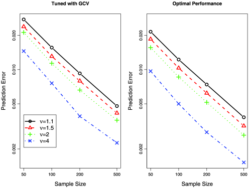
Figure 1: Prediction errors of the regularized estimator ($\sigma=0.5$): $X$ was simulated with a covariance function with well-spaced eigenvalues. The results are averaged over 1000 runs. Black solid lines, red dashed lines, green dotted lines and blue dash-dotted lines correspond to $\nu=1.1,\;1.5,\;2$ and $4$, respectively. Both axes are in log scale.

We begin with the setting of well-spaced eigenvalues. The left panel of Figure 1 shows the prediction error, $\|\hat{\beta}_{n\lambda}-\beta_{0}\|_{0}^{2}$, for each combination of $\nu$ value and sample size when $\sigma=0.5$. The results were averaged over 1000 simulation runs in each setting. Both axes are given in the log scale. The plot suggests that the estimation error converges at a polynomial rate as sample size $n$ increases, which agrees with our theoretical results from the previous section. Furthermore, one can observe that with the same sample size, the prediction error tends to be smaller for larger $\nu$. This also confirms our theoretical development which indicates that the faster the eigenvalues of the covariance operator for $X(\cdot)$ decay, the smaller the prediction error.

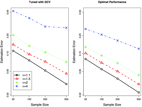
Figure 2: Estimation errors of the regularized estimator ($\sigma=0.5$): $X$ was simulated with a covariance function with well-spaced eigenvalues. The results are averaged over 1000 runs. Black solid lines, red dashed lines, green dotted lines and blue dash-dotted lines correspond to $\nu=1.1,1.5,2$ and $4$, respectively. Both axes are in log scale.

To better understand the performance of the smoothness regularized estimator and the GCV choice of the tuning parameter, we also recorded the performance of an oracle estimator whose tuning parameter is chosen to minimize the prediction error. This choice of the tuning parameter ensures the optimal performance of the regularized estimator. It is, however, noteworthy that this is not a legitimate statistical estimator since it depends on the knowledge of unknown slope function $\beta_{0}$. The right panel of Figure 1 shows the prediction error associated with this choice of tuning parameter. It behaves similarly to the estimate with $\lambda$ chosen by GCV. Note that the comparison between the two panels suggest that GCV generally leads to near optimal performance.

We now turn to the estimation error. Figure 2 shows the estimation errors, averaged over 1000 simulation runs, with $\lambda$ chosen by GCV or minimizing the estimation error for each combination of sample size and $\nu$ value. Similarly to the prediction error, the plots suggest a polynomial rate of convergence of the estimation error when the sample size increases, and GCV again leads to near-optimal choice of the tuning parameter.

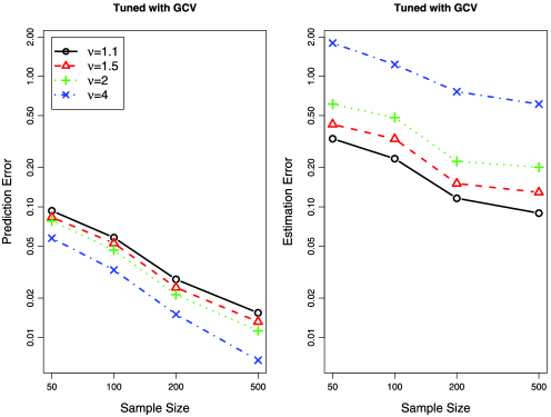
Figure 3: Estimation and prediction errors of the regularized estimator ($\sigma^{2}=1^{2}$): $X$ was simulated with a covariance function with well-spaced eigenvalues. The results are averaged over 1000 runs. Black solid lines, red dashed lines, green dotted lines and blue dash-dotted lines correspond to $\nu=1.1,1.5,2$ and $4$, respectively. Both axes are in log scale.

A comparison between Figures 1 and 2 suggests that when $X$ is smoother (larger $\nu$), prediction (as measured by the prediction error) is easier, but estimation (as measured by the estimation error) tends to be harder, which highlights the difference between prediction and estimation in functional linear regression. We also note that this observation is in agreement with our theoretical results from the previous section where it is shown that the estimation error decreases at the rate of $n^{-2r/(2(r+s)+1)}$ which decelerates as $s$ increases; whereas the prediction error decreases at the rate of $n^{-2(r+s)/(2(r+s)+1)}$ which accelerates as $s$ increases.

Figure 3 reports the prediction and estimation error when tuned with GCV for the large noise ($\sigma=1$) setting. Observations similar to those for the small noise setting can also be made. Furthermore, notice that the prediction errors are much smaller than the estimation error, which confirms our finding from the previous section that prediction is an easier problem in the context of functional linear regression.

The numerical results in the setting with closely spaced eigenvalues are qualitatively similar to those in the setting with well-spaced eigenvalues. Figure 4 summarizes the results obtained for the setting with closely spaced eigenvalues.

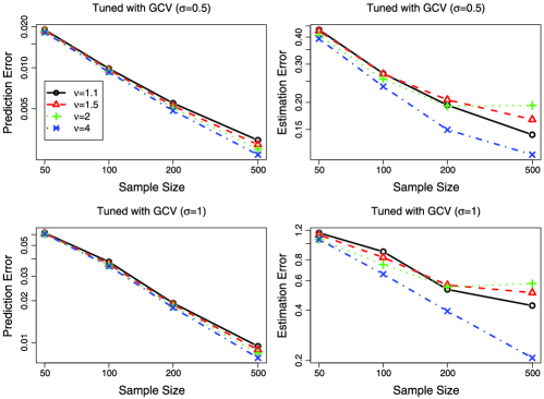
Figure 4: Estimation and prediction errors of the regularized estimator: $X$ was simulated with a covariance function with closely-spaced eigenvalues. The results are averaged over 1000 runs. Both axes are in log scale. Note that $y$-axes are of different scales across panels.

We also note that the performance of the regularization estimate with $\lambda$ tuned with GCV compares favorably with those from Hall and Horowitz (2007) using FPCA-based methods even though their results are obtained with optimal rather than data-driven choice of the tuning parameters.

6 Proofs

6.1 Proof of Proposition 2

Observe that

$$\int_{\mathcal{T}\times\mathcal{T}}f(s)C(s,t)f(t)\,ds\,dt\leq\mu_{1}\|f\|_{\mathcal{L}_{2}}^{2}\leq c_{1}\|f\|_{\mathcal{H}}^{2}$$ (59)

for some constant $c_{1}>0$. Together with the fact that $J(f)\leq\|f\|_{\mathcal{H}}^{2}$, we conclude that

$$\|f\|_{R}^{2}=\int_{\mathcal{T}\times\mathcal{T}}f(s)C(s,t)f(t)\,ds\,dt+J(f)\leq(c_{1}+1)\|f\|_{\mathcal{H}}^{2}.$$ (60)

Recall that $\xi_{k}$, $k=1,\ldots,N,$ are the orthonormal basis of $\mathcal{H}_{0}$. Under the assumption of the proposition, the matrix $\Sigma=(\langle C\xi_{j},\xi_{k}\rangle_{\mathcal{H}})_{1\leq j,k\leq N}$ is a positive definite matrix. Denote by $\mu_{1}^{\prime}\geq\mu_{2}^{\prime}\geq\cdots\geq\mu_{N}^{\prime}>0$ its eigenvalues. It is clear that for any $f_{0}\in\mathcal{H}_{0}$

$$\|f_{0}\|_{R}^{2}\geq\mu_{N}^{\prime}\|f_{0}\|_{\mathcal{H}}^{2}.$$ (61)

Note also that for any $f_{1}\in\mathcal{H}_{1}$,

$$\|f_{1}\|_{\mathcal{H}}^{2}=J(f_{1})\leq\|f_{1}\|_{R}^{2}.$$ (62)

For any $f\in\mathcal{H}$, we can write $f:=f_{0}+f_{1}$ where $f_{0}\in\mathcal{H}_{0}$ and $f_{1}\in\mathcal{H}_{1}$. Then

$$\|f\|_{R}^{2}=\int_{\mathcal{T}\times\mathcal{T}}f(s)C(s,t)f(t)\,ds\,dt+\|f_{1}\|_{\mathcal{H}}^{2}.$$ (63)

Recall that

$$\|f_{1}\|_{\mathcal{H}}^{2}\geq\rho_{1}^{-1}\|f_{1}\|_{\mathcal{L}_{2}}^{2}\geq\rho_{1}^{-1}\mu_{1}^{-1}\int_{\mathcal{T}\times\mathcal{T}}f_{0}(s)C(s,t)f_{0}(t)\,ds\,dt.$$ (64)

For brevity, assume that $\rho_{1}=\mu_{1}=1$ without loss of generality. By the Cauchy–Schwarz inequality,

$$\|f\|_{R}^{2} \geq {1\over 2}\int_{\mathcal{T}\times\mathcal{T}}f(s)C(s,t)f(t)\,ds\,dt+\|f_{1}\|_{\mathcal{H}}^{2}$$

$$\geq {1\over 2}\int_{\mathcal{T}\times\mathcal{T}}f_{0}(s)C(s,t)f_{0}(t)\,ds\,dt+{3\over 2}\int_{\mathcal{T}\times\mathcal{T}}f_{1}(s)C(s,t)f_{1}(t)\,ds\,dt$$

$${}-\biggl{(}\int_{\mathcal{T}\times\mathcal{T}}f_{0}(s)C(s,t)f_{0}(t)\,ds\,dt\biggr{)}^{1/2}$$

$$\hskip 12.0pt{}\times\biggl{(}\int_{\mathcal{T}\times\mathcal{T}}f_{1}(s)C(s,t)f_{1}(t)\,ds\,dt\biggr{)}^{1/2}$$

$$\geq {1\over 3}\int_{\mathcal{T}\times\mathcal{T}}f_{0}(s)C(s,t)f_{0}(t)\,ds\,dt,$$

where we used the fact that $3a^{2}/2-ab\geq-b^{2}/6$ in deriving the last inequality. Therefore,

$${3\over\mu_{N}^{\prime}}\|f\|_{R}^{2}\geq\|f_{0}\|_{\mathcal{H}}^{2}.$$ (65)

Together with the facts that $\|f\|_{\mathcal{H}}^{2}=\|f_{0}\|_{\mathcal{H}}^{2}+\|f_{1}\|_{\mathcal{H}}^{2}$ and

$$\|f\|_{R}^{2}\geq J(f_{1})\geq\|f_{1}\|_{\mathcal{H}}^{2},$$ (66)

we conclude that

$$\|f\|_{R}^{2}\geq(1+3/\mu_{N}^{\prime})^{-1}\|f\|_{\mathcal{H}}^{2}.$$ (67)

The proof is now complete.

6.2 Proof of Theorem 3

First note that

$$R^{-1/2}f = \sum_{k=1}^{\infty}\langle R^{-1/2}f,\zeta_{k}\rangle_{\mathcal{L}_{2}}\zeta_{k}=\sum_{k=1}^{\infty}\langle R^{-1/2}f,\nu_{k}^{1/2}R^{-1/2}\omega_{k}\rangle_{\mathcal{L}_{2}}\nu_{k}^{1/2}R^{-1/2}\omega_{k}$$

$$= R^{-1/2}\Biggl{(}\sum_{k=1}^{\infty}\nu_{k}\langle R^{-1/2}f,R^{-1/2}\omega_{k}\rangle_{\mathcal{L}_{2}}\omega_{k}\Biggr{)}=R^{-1/2}\Biggl{(}\sum_{k=1}^{\infty}\nu_{k}\langle f,\omega_{k}\rangle_{R}\omega_{k}\Biggr{)}.$$

Applying bounded positive definite operator $R^{1/2}$ to both sides leads to

$$f=\sum_{k=1}^{\infty}\nu_{k}\langle f,\omega_{k}\rangle_{R}\omega_{k}.$$ (68)

Recall that $\langle\omega_{k},\omega_{j}\rangle_{R}=\nu_{k}^{-1}\delta_{kj}$. Therefore,

$$\|f\|_{R}^{2} = \Bigg{\langle}\sum_{k=1}^{\infty}\nu_{k}\langle f,\omega_{k}\rangle_{R}\omega_{k},\sum_{j=1}^{\infty}\nu_{j}\langle f,\omega_{j}\rangle_{R}\omega_{j}\Bigg{\rangle}_{R}$$

$$= \sum_{k,j=1}\nu_{k}\nu_{j}\langle f,\omega_{k}\rangle_{R}\langle f,\omega_{j}\rangle_{R}\langle\omega_{k},\omega_{j}\rangle_{R}$$

$$= \sum_{k=1}\nu_{k}\langle f,\omega_{k}\rangle_{R}^{2}.$$

Similarly, because $\langle C\omega_{k},\omega_{j}\rangle_{\mathcal{L}_{2}}=\delta_{kj}$,

$$\langle Cf,f\rangle_{\mathcal{L}_{2}} = \Bigg{\langle}C\Biggl{(}\sum_{k=1}^{\infty}\nu_{k}\langle f,\omega_{k}\rangle_{R}\omega_{k}\Biggr{)},\sum_{j=1}^{\infty}\nu_{j}\langle f,\omega_{j}\rangle_{R}\omega_{j}\Bigg{\rangle}_{\mathcal{L}_{2}}$$

$$= \Bigg{\langle}\sum_{k=1}^{\infty}\nu_{k}\langle f,\omega_{k}\rangle_{R}C\omega_{k},\sum_{j=1}^{\infty}\nu_{j}\langle f,\omega_{j}\rangle_{R}\omega_{j}\Bigg{\rangle}_{\mathcal{L}_{2}}$$

$$= \sum_{k,j=1}\nu_{k}\nu_{j}\langle f,\omega_{k}\rangle_{R}\langle f,\omega_{j}\rangle_{R}\langle C\omega_{k},\omega_{j}\rangle_{\mathcal{L}_{2}}$$

$$= \sum_{k=1}\nu_{k}^{2}\langle f,\omega_{k}\rangle_{R}^{2}.$$

6.3 Proof of Proposition 4

Recall that for any $f\in\mathcal{H}_{0}$, $Cf\neq 0$ if and only if $f=0$, which implies that $\mathcal{H}_{0}\cap{\rm l.s.}\{\phi_{k}\dvtx k\geq 1\}^{\perp}=\{0\}$. Together with the fact that $\mathcal{H}_{0}\cap\mathcal{H}_{1}=\{0\}$, we conclude that $\mathcal{H}=\mathcal{H}_{1}={\rm l.s.}\{\phi_{k}\dvtx k\geq 1\}$. It is not hard to see that for any $f,g\in\mathcal{H}$,

$$\langle f,g\rangle_{R}=\int_{\mathcal{T}\times\mathcal{T}}f(s)C(s,t)g(t)\,ds\,dt+\langle f,g\rangle_{K}.$$ (69)

In particular,

$$\langle\psi_{j},\psi_{k}\rangle_{R}=(\mu_{k}+\rho_{k}^{-1})\delta_{jk},$$ (70)

which implies that $\{((\mu_{k}+\rho_{k}^{-1})^{-1},\psi_{k})\dvtx k\geq 1\}$ is also the eigen system of $R$, that is,

$$R(s,t)=\sum_{k=1}^{\infty}(\mu_{k}+\rho_{k}^{-1})^{-1}\psi_{k}(s)\psi_{k}(t).$$ (71)

Then

$$R\psi_{k}:=\int_{\mathcal{T}}R(\cdot,t)\psi_{k}(t)\,dt=(\mu_{k}+\rho_{k}^{-1})^{-1}\psi_{k},\qquad k=1,2,\ldots.$$ (72)

Therefore,

$$R^{1/2}CR^{1/2}\psi_{k} = R^{1/2}C\bigl{(}(\mu_{k}+\rho_{k}^{-1})^{-1/2}\psi_{k}\bigr{)}$$

$$= R^{1/2}\bigl{(}\mu_{k}(\mu_{k}+\rho_{k}^{-1})^{-1/2}\psi_{k}\bigr{)}=(1+\rho_{k}^{-1}\mu_{k}^{-1})^{-1}\psi_{k},$$

which implies that $\zeta_{k}=\psi_{k}=\phi_{k}$, $\nu_{k}=(1+\rho_{k}^{-1}\mu_{k}^{-1})^{-1}$ and $\gamma_{k}=\rho_{k}\mu_{k}$. Consequently,

$$\omega_{k}=\nu_{k}^{-1/2}R^{1/2}\psi_{k}=\nu_{k}^{-1/2}(\mu_{k}+\rho_{k}^{-1})^{-1/2}\psi_{k}=\mu_{k}^{-1/2}\psi_{k}.$$ (73)

6.4 Proof of Theorem 5

Recall that $\mathcal{H}=\mathcal{W}_{2}^{m}$, which implies that $\rho_{k}\asymp k^{-2m}$. By Corollary 2 of Ritter, Wasilkowski and Woźniakowski (1995), $\mu_{k}\asymp k^{-2(s+1)}$. It therefore suffices to show $\gamma_{k}\asymp k^{-2(s+1+m)}$. The key idea of the proof is a result from Ritter, Wasilkowski and Woźniakowski (1995) indicating that the reproducing kernel Hilbert space associated with $C$ differs from $\mathcal{W}^{s+1}_{2}([0,1])$ only by a finite-dimensional linear space of polynomials.

Denote by $Q_{r}$ the reproducing kernel for $\mathcal{W}^{r}_{2}([0,1])$. Observe that $Q_{r}^{1/2}(\mathcal{L}_{2})=\mathcal{W}^{r}_{2}$ [e.g., Cucker and Smale (2001)]. We begin by quantifying the decay rate of $\lambda_{k}(Q_{m}^{1/2}Q_{s+1}Q_{m}^{1/2})$. By Sobolev’s embedding theorem, $(Q_{s+1}^{1/2}Q_{m}^{1/2})(\mathcal{L}_{2})=Q_{s+1}^{1/2}(\mathcal{W}_{2}^{m})=\mathcal{W}_{2}^{m+s+1}$. Therefore, $Q_{m}^{1/2}Q_{s+1}Q_{m}^{1/2}$ is equivalent to $Q_{m+s+1}$. Denote by $\lambda_{k}(Q)$ be the $k$th largest eigenvalue of a positive definite operator $Q$. Let $\{h_{k}\dvtx k\geq 1\}$ be the eigenfunctions of $Q_{m+s+1}$, that is, $Q_{m+s+1}h_{k}=\lambda_{k}(Q_{m+s+1})h_{k}$, $k=1,2,\ldots.$ Denote by $\mathcal{F}_{k}$ and $\mathcal{F}_{k}^{\perp}$ the linear space spanned by $\{h_{j}\dvtx 1\leq j\leq k\}$ and $\{h_{j}\dvtx j\geq k+1\}$, respectively. By the Courant–Fischer–Weyl min–max principle,

$$\lambda_{k}(Q_{m}^{1/2}Q_{s+1}Q_{m}^{1/2}) \geq \min_{f\in\mathcal{F}_{k}}\|Q_{s+1}^{1/2}Q_{m}^{1/2}f\|_{\mathcal{L}_{2}}^{2}/\|f\|_{\mathcal{L}_{2}}^{2}$$

$$\geq C_{1}\min_{f\in\mathcal{F}_{k}}\|Q_{m+s+1}^{1/2}f\|_{\mathcal{L}_{2}}^{2}/\|f\|_{\mathcal{L}_{2}}^{2}$$

$$\geq C_{1}\lambda_{k}(Q_{m+s+1})$$

for some constant $C_{1}>0$. On the other hand,

$$\lambda_{k}(Q_{m}^{1/2}Q_{s+1}Q_{m}^{1/2}) \leq \max_{f\in\mathcal{F}_{k-1}^{\perp}}\|Q_{s+1}^{1/2}Q_{m}^{1/2}f\|_{\mathcal{L}_{2}}^{2}/\|f\|_{\mathcal{L}_{2}}^{2}$$

$$\leq C_{2}\min_{f\in\mathcal{F}_{k-1}^{\perp}}\|Q_{m+s+1}^{1/2}f\|_{\mathcal{L}_{2}}^{2}/\|f\|_{\mathcal{L}_{2}}^{2}$$

$$\leq C_{2}\lambda_{k}(Q_{m+s+1})$$

for some constant $C_{2}>0$. In summary, we have $\lambda_{k}(Q_{m}^{1/2}Q_{s+1}Q_{m}^{1/2})\asymp\break\times k^{-2(m+s+1)}$.

As shown by Ritter, Wasilkowski and Woźniakowski [(1995), Theorem 1, page 525], there exist $D$ and $U$ such that $Q_{s+1}=D+U$, $D$ has at most $2(s+1)$ nonzero eigenvalues and $\|U^{1/2}f\|_{\mathcal{L}_{2}}$ is equivalent to $\|C^{1/2}f\|_{\mathcal{L}_{2}}$. Moreover, the eigenfunctions of $D$, denoted by $\{g_{1},\ldots,g_{d}\}$ ($d\leq 2(s+1)$) are polynomials of order no greater than $2s+1$. Denote $\mathcal{G}$ the space spanned by $\{g_{1},\ldots,g_{d}\}$. Clearly $\mathcal{G}\subset\mathcal{W}_{2}^{m}=Q_{m}^{1/2}(\mathcal{L}_{2})$. Denote $\{\tilde{h}_{j}\dvtx j\geq 1\}$ the eigenfunctions of $Q_{m}^{1/2}Q_{s+1}Q_{m}^{1/2}$. Let $\tilde{\mathcal{F}}_{k}$ and $\tilde{\mathcal{F}}_{k}^{\perp}$ be defined similarly as $\mathcal{F}_{k}$ and $\mathcal{F}_{k}^{\perp}$. Then by the Courant–Fischer–Weyl min–max principle,

$$\lambda_{k-d}(Q_{m}^{1/2}UQ_{m}^{1/2}) \geq \min_{f\in\tilde{\mathcal{F}}_{k}\cap Q_{m}^{-1/2}(\mathcal{G})^{\perp}}\|U^{1/2}Q_{m}^{1/2}f\|_{\mathcal{L}_{2}}^{2}/\|f\|_{\mathcal{L}_{2}}^{2}$$

$$= \min_{f\in\tilde{\mathcal{F}}_{k}\cap Q_{m}^{-1/2}(\mathcal{G})^{\perp}}\|Q_{s+1}^{1/2}Q_{m}^{1/2}f\|_{\mathcal{L}_{2}}^{2}/\|f\|_{\mathcal{L}_{2}}^{2}$$

$$= \min_{f\in\tilde{\mathcal{F}}_{k}}\|Q_{s+1}^{1/2}Q_{m}^{1/2}f\|_{\mathcal{L}_{2}}^{2}/\|f\|_{\mathcal{L}_{2}}^{2}$$

$$\geq C_{1}\lambda_{k}(Q_{m+s+1})$$

for some constant $C_{1}>0$. On the other hand,

$$\lambda_{k+d}(Q_{m}^{1/2}Q_{s+1}Q_{m}^{1/2}) \leq \max_{f\in\tilde{\mathcal{F}}_{k-1}^{\perp}\cap Q_{m}^{-1/2}(\mathcal{G})^{\perp}}\|U^{1/2}Q_{m}^{1/2}f\|_{\mathcal{L}_{2}}^{2}/\|f\|_{\mathcal{L}_{2}}^{2}$$

$$= \max_{f\in\tilde{\mathcal{F}}_{k-1}^{\perp}\cap Q_{m}^{-1/2}(\mathcal{G})^{\perp}}\|Q_{s+1}^{1/2}Q_{m}^{1/2}f\|_{\mathcal{L}_{2}}^{2}/\|f\|_{\mathcal{L}_{2}}^{2}$$

$$= \min_{f\in\tilde{\mathcal{F}}_{k-1}^{\perp}}\|Q_{s+1}^{1/2}Q_{m}^{1/2}f\|_{\mathcal{L}_{2}}^{2}/\|f\|_{\mathcal{L}_{2}}^{2}$$

$$\leq C_{2}\lambda_{k}(Q_{m+s+1})$$

for some constant $C_{2}>0$. Hence $\lambda_{k}(Q_{m}^{1/2}UQ_{m}^{1/2})\asymp k^{-2(m+s+1)}$.

Because $Q_{m}^{1/2}UQ_{m}^{1/2}$ is equivalent to $R^{1/2}CR^{1/2}$, following a similar argument as before, by the Courant–Fischer–Weyl min–max principle, we complete the the proof.

6.5 Proof of Theorem 6

We now proceed to prove Theorem 6. The analysis follows a similar spirit as the technique commonly used in the study of the rate of convergence of smoothing splines [see, e.g., Silverman (1982); Cox and O’Sullivan (1990)]. For brevity, we shall assume that $EX(\cdot)=0$ in the rest of the proof. In this case, $\alpha_{0}$ can be estimated by $\bar{y}$ and $\beta_{0}$ by

$$\hat{\beta}_{n\lambda}=\mathop{\arg\min}_{\beta\in\mathcal{H}}\Biggl{[}{1\over n}\sum_{i=1}^{n}\biggl{(}y_{i}-\int_{\mathcal{T}}x_{i}(t)\beta(t)\,dt\biggr{)}^{2}+\lambda J(\beta)\Biggr{]}.$$ (74)

The proof below also applies to the more general setting when $EX(\cdot)\neq 0$ but with considerable technical obscurity.

Recall that

$$\ell_{n}(\beta)={1\over n}\sum_{i=1}^{n}\biggl{(}y_{i}-\int_{\mathcal{T}}x_{i}(t)\beta(t)\,dt\biggr{)}^{2}.$$ (75)

Observe that

$$\ell_{\infty}(\beta) := E\ell_{n}(\beta)=E\biggl{[}Y-\int_{\mathcal{T}}X(t)\beta(t)\,dt\biggr{]}^{2}$$

$$= \sigma^{2}+\int_{\mathcal{T}}\int_{\mathcal{T}}[\beta(s)-\beta_{0}(s)]C(s,t)[\beta(t)-\beta_{0}(t)]\,ds\,dt$$

$$= \sigma^{2}+\|\beta-\beta_{0}\|^{2}_{0}.$$

Write

$$\bar{\beta}_{\infty\lambda}=\mathop{\arg\min}_{\beta\in\mathcal{H}}\{\ell_{\infty}(\beta)+\lambda J(\beta)\}.$$ (76)

Clearly

$$\hat{\beta}_{n\lambda}-\beta_{0}=(\hat{\beta}_{n\lambda}-\bar{\beta}_{\infty\lambda})+(\bar{\beta}_{\infty\lambda}-\beta_{0}).$$ (77)

We refer to the two terms on the right-hand side stochastic error and deterministic error, respectively.

6.5.1 Deterministic error

Write $\beta_{0}(\cdot)=\sum_{k=1}^{\infty}a_{k}\omega_{k}(\cdot)$ and ${\beta}(\cdot)=\break\sum_{k=1}^{\infty}b_{k}\omega_{k}(\cdot)$. Then Theorem 3 implies that

$$\ell_{\infty}({\beta})=\sigma^{2}+\sum_{k=1}^{\infty}(b_{k}-{a}_{k})^{2},\qquad J({\beta})=\sum_{k=1}^{\infty}\gamma_{k}^{-1}b_{k}^{2}.$$

Therefore,

$$\bar{\beta}_{\infty\lambda}(\cdot)=\sum_{k=1}^{\infty}{a_{k}\over 1+\lambda\gamma_{k}^{-1}}\omega_{k}(\cdot)=:\sum_{k=1}^{\infty}\bar{b}_{k}\omega_{k}(\cdot).$$ (78)

It can then be computed that for any $a<1$,

$$\|\bar{\beta}_{\infty\lambda}-\beta_{0}\|_{a}^{2} = \sum_{k=1}^{\infty}(1+\gamma_{k}^{-a})(\bar{b}_{k}-a_{k})^{2}$$

$$= \sum_{k=1}^{\infty}(1+\gamma_{k}^{-a})\biggl{(}{\lambda\gamma_{k}^{-1}\over 1+\lambda\gamma_{k}^{-1}}\biggr{)}^{2}a_{k}^{2}$$

$$\leq \lambda^{2}\sup_{k}{(1+\gamma^{-a})\gamma_{k}^{-1}\over(1+\lambda\gamma_{k}^{-1})^{2}}\sum_{k=1}^{\infty}\gamma_{k}^{-1}a_{k}^{2}$$

$$= \lambda^{2}J(\beta_{0})\sup_{k}{(1+\gamma^{-a})\gamma_{k}^{-1}\over(1+\lambda\gamma_{k}^{-1})^{2}}.$$

Now note that

$$\sup_{k}{(1+\gamma^{-a})\gamma_{k}^{-1}\over(1+\lambda\gamma_{k}^{-1})^{2}} \leq \sup_{x>0}{(1+x^{-a})x^{-1}\over(1+\lambda x^{-1})^{2}}$$

$$\leq \sup_{x>0}{x^{-1}\over(1+\lambda x^{-1})^{2}}+\sup_{x>0}{x^{-(a+1)}\over(1+\lambda x^{-1})^{2}}$$

$$= {1\over\inf_{x>0}(x^{1/2}+\lambda x^{-1/2})^{2}}+{1\over\inf_{x>0}(x^{(a+1)/2}+\lambda x^{-(1-a)/2})^{2}}$$

$$= {1\over 4\lambda}+C_{0}\lambda^{-(a+1)}.$$

Hereafter, we use $C_{0}$ to denote a generic positive constant. In summary, we have

Lemma 12

If $\lambda$ is bounded from above, then

$$\|\bar{\beta}_{\infty\lambda}-\beta_{0}\|^{2}_{a}=O({\lambda^{1-a}}J(\beta_{0})).$$

6.5.2 Stochastic error

Next, we consider the stochastic error $\hat{\beta}_{n\lambda}-\bar{\beta}_{\infty\lambda}$. Denote

$$D\ell_{n}(\beta)f = -{2\over n}\sum_{i=1}^{n}\biggl{[}\biggl{(}y_{i}-\int_{\mathcal{T}}x_{i}(t)\beta(t)\,dt\biggr{)}\int_{\mathcal{T}}x_{i}(t)f(t)\,dt\biggr{]},$$

$$D\ell_{\infty}(\beta)f = -2E_{X}\biggl{(}\int_{\mathcal{T}}X(t)[\beta_{0}(t)-\beta(t)]\,dt\int_{\mathcal{T}}X(t)f(t)\,dt\biggr{)}$$

$$= -2\int_{\mathcal{T}}\int_{\mathcal{T}}[\beta_{0}(s)-\beta(s)]C(s,t)f(t)\,ds\,dt,$$

$$D^{2}\ell_{n}(\beta)fg = {2\over n}\sum_{i=1}^{n}\biggl{[}\int_{\mathcal{T}}x_{i}(t)f(t)\,dt\int_{\mathcal{T}}x_{i}(t)g(t)\,dt\biggr{]},$$

$$D^{2}\ell_{\infty}(\beta)fg = 2\int_{\mathcal{T}}\int_{\mathcal{T}}f(s)C(s,t)g(t)\,ds\,dt.$$

Also write $\ell_{n\lambda}(\beta)=\ell_{n}(\beta)+\lambda J(\beta)$ and $\ell_{\infty\lambda}=\ell_{\infty}(\beta)+\lambda J(\beta)$. Denote $G_{\lambda}=(1/2)D^{2}\ell_{\infty\lambda}(\bar{\beta}_{\infty\lambda})$ and

$$\tilde{\beta}=\bar{\beta}_{\infty\lambda}-\tfrac 12G_{\lambda}^{-1}D\ell_{n\lambda}(\bar{\beta}_{\infty\lambda}).$$ (79)

It is clear that

$$\hat{\beta}_{n\lambda}-\bar{\beta}_{\infty\lambda}=(\hat{\beta}_{n\lambda}-\tilde{\beta})+(\tilde{\beta}-\bar{\beta}_{\infty\lambda}).$$ (80)

We now study the two terms on the right-hand side separately. For brevity, we shall abbreviate the subscripts of $\hat{\beta}$ and $\bar{\beta}$ in what follows. We begin with $\tilde{\beta}-\bar{\beta}$. Hereafter we shall omit the subscript for brevity if no confusion occurs.

Lemma 13

For any $0\leq a\leq 1$,

$$E\|\tilde{\beta}-\bar{\beta}\|_{a}^{2}\asymp n^{-1}\lambda^{-(a+1/(2(r+s)))}.$$ (81)

Notice that $D\ell_{n\lambda}(\bar{\beta})=D\ell_{n\lambda}(\bar{\beta})-D\ell_{\infty\lambda}(\bar{\beta})=D\ell_{n}(\bar{\beta})-D\ell_{\infty}(\bar{\beta})$. Therefore

$$E[D\ell_{n\lambda}(\bar{\beta})f]^{2} = E[D\ell_{n}(\bar{\beta})f-D\ell_{\infty}(\bar{\beta})f]^{2}$$

$$= {4\over n}\operatorname{Var}\biggl{[}\biggl{(}Y-\int_{\mathcal{T}}X(t)\bar{\beta}(t)\,dt\biggr{)}\int_{\mathcal{T}}X(t)f(t)\,dt\biggr{]}$$

$$\leq {4\over n}E\biggl{[}\biggl{(}Y-\int_{\mathcal{T}}X(t)\bar{\beta}(t)\,dt\biggr{)}\int_{\mathcal{T}}X(t)f(t)\,dt\biggr{]}^{2}$$

$$= {4\over n}E\biggl{(}\int_{\mathcal{T}}X(t)[\beta_{0}(t)-\bar{\beta}(t)]\,dt\int_{\mathcal{T}}X(t)f(t)\,dt\biggr{)}^{2}$$

$${}+{4\sigma^{2}\over n}E\biggl{(}\int_{\mathcal{T}}X(t)f(t)\,dt\biggr{)}^{2},$$

where we used the fact that $\varepsilon=Y-\int X\beta_{0}$ is uncorrelated with $X$. To bound the first term, an application of the Cauchy–Schwarz inequality yields

$$E\biggl{(}\int_{\mathcal{T}}X(t)[\beta_{0}(t)-\bar{\beta}(t)]\,dt\int_{\mathcal{T}}X(t)f(t)\,dt\biggr{)}^{2}$$

$$\qquad\leq\biggl{\{}E\biggl{(}\int_{\mathcal{T}}X(t)[\beta_{0}(t)-\bar{\beta}(t)]\,dt\biggr{)}^{4}E\biggl{(}\int_{\mathcal{T}}X(t)f(t)\,dt\biggr{)}^{4}\biggr{\}}^{1/2}$$

$$\qquad\leq M\|\beta_{0}-\bar{\beta}\|^{2}_{0}\|f\|_{0}^{2},$$

where the second inequality holds by the second condition of $\mathcal{F}(s,M,K)$. Therefore,

$$E[D\ell_{n\lambda}(\bar{\beta})f]^{2}\leq{4M\over n}\|\beta_{0}-\bar{\beta}\|^{2}_{0}\|f\|_{0}^{2}+{4\sigma^{2}\over n}\|f\|_{0}^{2},$$ (82)

which by Lemma 12 is further bounded by $(C_{0}\sigma^{2}/n)\|f\|_{0}^{2}$ for some positive constant $C_{0}$. Recall that $\|\omega_{k}\|_{0}=1$. We have

$$E[D\ell_{n\lambda}(\bar{\beta})\omega_{k}]^{2}\leq C_{0}\sigma^{2}/n.$$ (83)

Thus, by the definition of $\tilde{\beta}$,

$$E\|\tilde{\beta}-\bar{\beta}\|_{a}^{2} = E\bigg{\|}{1\over 2}G_{\lambda}^{-1}D\ell_{n\lambda}(\bar{\beta})\bigg{\|}_{a}^{2}$$

$$= {1\over 4}E\Biggl{[}\sum_{k=1}^{\infty}(1+\gamma_{k}^{-a})(1+\lambda\gamma_{k}^{-1})^{-2}(D\ell_{n\lambda}(\bar{\beta})\omega_{k})^{2}\Biggr{]}$$

$$\leq {C_{0}\sigma^{2}\over 4n}\sum_{k=1}^{\infty}(1+\gamma_{k}^{-a})(1+\lambda\gamma_{k}^{-1})^{-2}$$

$$\leq {C_{0}\sigma^{2}\over 4n}\sum_{k=1}^{\infty}\bigl{(}1+k^{2a(r+s)}\bigr{)}\bigl{(}1+\lambda k^{2(r+s)}\bigr{)}^{-2}$$

$$\asymp {C_{0}\sigma^{2}\over 4n}\int_{1}^{\infty}x^{2a(r+s)}\bigl{(}1+\lambda x^{2(r+s)}\bigr{)}^{-2}\,dx$$

$$\asymp {C_{0}\sigma^{2}\over 4n}\int_{1}^{\infty}\bigl{(}1+\lambda x^{2(r+s)/(2a(r+s)+1)}\bigr{)}^{-2}\,dx$$

$$= {C_{0}\sigma^{2}\over 4n}\lambda^{-(a+1/(2(r+s)))}\int_{\lambda^{a+1/(2(r+s))}}^{\infty}\bigl{(}1+x^{2(r+s)/(2a(r+s)+1)}\bigr{)}^{-2}\,dx$$

$$\asymp n^{-1}\lambda^{-(a+1/(2(r+s)))}.$$

The proof is now complete.

Now we are in position to bound $E\|\hat{\beta}-\tilde{\beta}\|_{a}^{2}$. By definition,

$$G_{\lambda}(\hat{\beta}-\tilde{\beta})=\tfrac 12D^{2}\ell_{\infty\lambda}(\bar{\beta})(\hat{\beta}-\tilde{\beta}).$$ (84)

First-order condition implies that

$$D\ell_{n\lambda}(\hat{\beta})=D\ell_{n\lambda}(\bar{\beta})+D^{2}\ell_{n\lambda}(\bar{\beta})(\hat{\beta}-\bar{\beta})=0,$$ (85)

where we used the fact that $\ell_{n,\lambda}$ is quadratic. Together with the fact that

$$D\ell_{n\lambda}(\bar{\beta})+D^{2}\ell_{\infty\lambda}(\bar{\beta})(\tilde{\beta}-\bar{\beta})=0,$$ (86)

we have

$$D^{2}\ell_{\infty\lambda}(\bar{\beta})(\hat{\beta}-\tilde{\beta}) = D^{2}\ell_{\infty\lambda}(\bar{\beta})(\hat{\beta}-\bar{\beta})+D^{2}\ell_{\infty\lambda}(\bar{\beta})(\bar{\beta}-\tilde{\beta})$$

$$= D^{2}\ell_{\infty\lambda}(\bar{\beta})(\hat{\beta}-\bar{\beta})-D^{2}\ell_{n\lambda}(\bar{\beta})(\hat{\beta}-\bar{\beta})$$

$$= D^{2}\ell_{\infty}(\bar{\beta})(\hat{\beta}-\bar{\beta})-D^{2}\ell_{n}(\bar{\beta})(\hat{\beta}-\bar{\beta}).$$

Therefore,

$$(\hat{\beta}-\tilde{\beta})=\tfrac 12G_{\lambda}^{-1}[D^{2}\ell_{\infty}(\bar{\beta})(\hat{\beta}-\bar{\beta})-D^{2}\ell_{n}(\bar{\beta})(\hat{\beta}-\bar{\beta})].$$ (87)

Write

$$\hat{\beta}=\sum_{k=1}^{\infty}\hat{b}_{k}\omega_{k}\quad\mbox{and}\quad\bar{\beta}=\sum_{k=0}^{\infty}\bar{b}_{k}\omega_{k}.$$ (88)

Then

$$\|\hat{\beta}-\tilde{\beta}\|^{2}_{a}$$

$$\qquad={1\over 4}\sum_{k=1}^{\infty}(1+\lambda\gamma_{k}^{-1})^{-2}(1+\gamma_{k}^{-a})$$

$$\qquad\quad\hskip 23.0pt{}\times\Biggl{[}\sum_{j=1}^{\infty}(\hat{b}_{j}-\bar{b}_{j})\int_{\mathcal{T}}\int_{\mathcal{T}}\omega_{j}(s)\Biggl{(}{1\over n}\sum_{i=1}^{n}x_{i}(t)x_{i}(s)-C(s,t)\Biggr{)}$$

$$\qquad\quad\hskip 217.0pt{}\times\omega_{k}(t)\,ds\,dt\Biggr{]}^{2}$$

$$\qquad\leq{1\over 4}\sum_{k=1}^{\infty}(1+\lambda\gamma_{k}^{-1})^{-2}(1+\gamma_{k}^{-a})\Biggl{[}\sum_{j=1}^{\infty}(\hat{b}_{j}-\bar{b}_{j})^{2}(1+\gamma_{j}^{-c})\Biggr{]}$$

$$\qquad\quad\hskip 23.0pt{}\times\Biggl{(}\sum_{j=1}^{\infty}(1+\gamma_{j}^{-c})^{-1}\Biggl{[}\int_{\mathcal{T}}\int_{\mathcal{T}}\omega_{j}(s)\Biggl{(}{1\over n}\sum_{i=1}^{n}x_{i}(t)x_{i}(s)-C(s,t)\Biggr{)}$$

$$\qquad\quad\hskip 236.0pt{}\times\omega_{k}(t)\,ds\,dt\Biggr{]}^{2}\Biggr{)},$$

where the inequality is due to the Cauchy–Schwarz inequality.

Note that

$$E\Biggl{(}\sum_{j=1}^{\infty}(1+\gamma_{j}^{-c})^{-1}\Biggl{[}\int_{\mathcal{T}}\omega_{j}(s)\Biggl{(}{1\over n}\sum_{i=1}^{n}x_{i}(t)x_{i}(s)-C(s,t)\Biggr{)}\omega_{k}(t)\,ds\,dt\Biggr{]}^{2}\Biggr{)}$$

$$\qquad={1\over n}\sum_{j=1}^{\infty}(1+\gamma_{j}^{-c})^{-1}\operatorname{Var}\biggl{(}\int_{\mathcal{T}}\omega_{j}(t)X(t)\,dt\,\int_{\mathcal{T}}\omega_{k}(t)X(t)\,dt\biggr{)}$$

$$\qquad\leq{1\over n}\sum_{j=1}^{\infty}(1+\gamma_{j}^{-c})^{-1}E\biggl{[}\biggl{(}\int_{\mathcal{T}}\omega_{j}(t)X(t)\,dt\biggr{)}^{2}\biggl{(}\int_{\mathcal{T}}\omega_{k}(t)X(t)\,dt\biggr{)}^{2}\biggr{]}$$

$$\qquad\leq{1\over n}\sum_{j=1}^{\infty}(1+\gamma_{j}^{-c})^{-1}E\biggl{[}\biggl{(}\int_{\mathcal{T}}\omega_{j}(t)X(t)\,dt\biggr{)}^{4}\biggr{]}^{1/2}E\biggl{[}\biggl{(}\int_{\mathcal{T}}\omega_{k}(t)X(t)\,dt\biggr{)}^{4}\biggr{]}^{1/2}$$

$$\qquad\leq{M\over n}\sum_{j=1}^{\infty}(1+\gamma_{j}^{-c})^{-1}E\biggl{[}\biggl{(}\int_{\mathcal{T}}\omega_{j}(t)X(t)\,dt\biggr{)}^{2}\biggr{]}E\biggl{[}\biggl{(}\int_{\mathcal{T}}\omega_{k}(t)X(t)\,dt\biggr{)}^{2}\biggr{]}$$

$$\qquad={M\over n}\sum_{j=1}^{\infty}(1+\gamma_{j}^{-c})^{-1}\asymp n^{-1},$$

provided that $c>1/2(r+s)$. On the other hand,

$$\sum_{k=1}^{\infty}(1+\lambda\gamma_{k}^{-1})^{-2}(1+\gamma_{k}^{-a})$$

$$\qquad\leq C_{0}\sum_{k=1}^{\infty}\bigl{(}1+\lambda k^{2(r+s)}\bigr{)}^{-2}\bigl{(}1+k^{2a(r+s)}\bigr{)}$$

$$\qquad\asymp\int_{1}^{\infty}\bigl{(}1+\lambda x^{2(r+s)}\bigr{)}^{-2}x^{2a(r+s)}\,dx$$

$$\qquad\asymp\int_{1}^{\infty}\bigl{(}1+\lambda x^{2(r+s)/(2a(r+s)+1)}\bigr{)}^{-2}\,dx$$

$$\qquad=\lambda^{-(a+1/(2(r+s)))}\int_{\lambda^{a+1/(2(r+s))}}^{\infty}\bigl{(}1+x^{2(r+s)/(2a(r+s)+1)}\bigr{)}^{-2}\,dx$$

$$\qquad\asymp\lambda^{-(a+1/(2(r+s)))}.$$

To sum up,

$$\|\hat{\beta}-\tilde{\beta}\|^{2}_{a}=O_{p}\bigl{(}n^{-1}\lambda^{-(a+1/(2(r+s)))}\|\hat{\beta}-\bar{\beta}\|^{2}_{c}\bigr{)}.$$ (89)

In particular, taking $a=c$ yields

$$\|\hat{\beta}-\tilde{\beta}\|^{2}_{c}=O_{p}\bigl{(}n^{-1}\lambda^{-(c+1/(2(r+s)))}\|\hat{\beta}-\bar{\beta}\|^{2}_{c}\bigr{)}.$$ (90)

If

$$n^{-1}\lambda^{-(c+1/(2(r+s)))}\to 0,$$ (91)

then

$$\|\hat{\beta}-\tilde{\beta}\|_{c}=o_{p}(\|\hat{\beta}-\bar{\beta}\|_{c}).$$ (92)

Together with the triangular inequality

$$\|\tilde{\beta}-\bar{\beta}\|_{c}\geq\|\hat{\beta}-\bar{\beta}\|_{c}-\|\hat{\beta}-\tilde{\beta}\|_{c}=\bigl{(}1-o_{p}(1)\bigr{)}\|\hat{\beta}-\bar{\beta}\|_{c}.$$ (93)

Therefore,

$$\|\hat{\beta}-\bar{\beta}\|_{c}=O_{p}(\|\tilde{\beta}-\bar{\beta}\|_{c})$$ (94)

Together with Lemma 13, we have

$$\|\hat{\beta}-\bar{\beta}\|^{2}_{c}=O_{p}\bigl{(}n^{-1}\lambda^{-(c+1/(2(r+s)))}\bigr{)}=o_{p}(1).$$ (95)

Putting it back to (89), we now have:

Lemma 14

If there also exists some ${1/2(r+s)}<c\leq 1$ such that $n^{-1}\times\lambda^{-(c+{1/2(r+s)})}\to 0$, then

$$\|\hat{\beta}-\tilde{\beta}\|^{2}_{a}=o_{p}\bigl{(}n^{-1}\lambda^{-(a+{1/2(r+s)})}\bigr{)}.$$ (96)

Combining Lemmas 12–14, we have

$$\lim_{D\to\infty}\mathop{\overline{\lim}}_{n\to\infty}\sup_{F\in\mathcal{F}(s,M,K),\beta_{0}\in\mathcal{H}}P\bigl{(}\|\hat{\beta}_{n\lambda}-\beta_{0}\|_{a}^{2}>Dn^{-2(1-a)(r+s)/(2(r+s)+1)}\bigr{)}$$

$$\qquad=0$$

by taking $\lambda\asymp n^{-2(r+s)/(2(r+s)+1)}$.

6.6 Proof of Theorem 7

We now set out to show that $n^{-2(1-a)(r+s)/(2(r+s)+1)}$ is the optimal rate. It follows from a similar argument as that of Hall and Horowitz (2007). Consider a setting where $\psi_{k}=\phi_{k}$, $k=1,2,\ldots.$ Clearly in this case we also have $\omega_{k}=\mu_{k}^{-1/2}\phi_{k}$. It suffices to show that the rate is optimal in this special case. Recall that $\beta_{0}=\sum a_{k}\phi_{k}$. Set

$$a_{k}=\cases{L_{n}^{-1/2}k^{-r}\theta_{k},&\quad$L_{n}+1\leq k\leq 2L_{n}$,\cr 0,&\quad\mbox{otherwise},}$$ (98)

where $L_{n}$ is the integer part of $n^{1/(2(r+s)+1)}$, and $\theta_{k}$ is either $0$ or $1$. It is clear that

$$\|\beta_{0}\|_{K}^{2}\leq\sum_{k=L_{n}+1}^{2L_{n}}L_{n}^{-1}=1.$$ (99)

Therefore $\beta_{0}\in\mathcal{H}$. Now let $X$ admit the following expansion: $X=\sum_{k}\xi_{k}k^{-s}\phi_{k}$ where $\xi_{k}$s are independent random variables drawn from a uniform distribution on $[-\sqrt{3},\sqrt{3}]$. Simple algebraic manipulation shows that the distribution of $X$ belongs to $\mathcal{F}(s,3)$. The observed data are

$$y_{i}=\sum_{k=L_{n}+1}^{2L_{n}}L_{n}^{-1/2}k^{-(r+s)}\xi_{ik}\theta_{k}+\varepsilon_{i},\qquad i=1,\ldots,n,$$ (100)

where the noise $\varepsilon_{i}$ is assumed to be independently sampled from $N(0,M_{2})$. As shown in Hall and Horowitz (2007),

$$\lim_{n\to\infty}\inf_{L_{n}<j\leq 2L_{n}}\inf_{\tilde{\theta}_{j}}\sup^{\ast}E(\tilde{\theta}_{j}-\theta_{j})^{2}>0,$$ (101)

where $\mathop{\sup}\limits^{*}$ denotes the supremum over all $2^{L_{n}}$ choices of $(\theta_{L_{n}+1},\ldots,\theta_{2L_{n}})$, and $\inf_{\tilde{\theta}}$ is taken over all measurable functions $\tilde{\theta}_{j}$ of the data. Therefore, for any estimate $\tilde{\beta}$,

$$\sup^{\ast}\|\tilde{\beta}-\beta_{0}\|_{a}^{2} = \sup^{\ast}\sum_{k=L_{n}+1}^{2L_{n}}L_{n}^{-1}k^{-2(1-a)(r+s)}E(\tilde{\theta}_{j}-\theta_{j})^{2}$$

$$\geq Mn^{-2(1-a)(r+s)/(2(r+s)+1)}$$

for some constant $M>0$.

Denote

$$\tilde{\tilde{\theta}}_{k}=\cases{1,&\quad$\tilde{\theta}_{k}>1$,\cr\tilde{\theta}_{k},&\quad$0\leq\tilde{\theta}_{k}\leq 1$,\cr 0,&\quad$\tilde{\theta}_{k}<0$.}$$ (103)

It is easy to see that

$$\sum_{k=L_{n}+1}^{2L_{n}}L_{n}^{-1}k^{-2(1-a)(r+s)}(\tilde{\theta}_{j}-\theta_{j})^{2}$$

(104)

$$\qquad\geq\sum_{k=L_{n}+1}^{2L_{n}}L_{n}^{-1}k^{-2(1-a)(r+s)}(\hskip 2.0pt\tilde{\tilde{\theta}}_{j}-\theta_{j})^{2}.$$

Hence, we can assume that $0\leq\tilde{\theta}_{j}\leq 1$ without loss of generality in establishing the lower bound. Subsequently,

$$\sum_{k=L_{n}+1}^{2L_{n}}L_{n}^{-1}k^{-2(1-a)(r+s)}(\tilde{\theta}_{j}-\theta_{j})^{2} \leq \sum_{k=L_{n}+1}^{2L_{n}}L_{n}^{-1}k^{-2(1-a)(r+s)}$$

$$\leq L_{n}^{-2(1-a)(r+s)}.$$

Together with (6.6), this implies that

$$\lim_{n\to\infty}\inf_{\tilde{\beta}}\sup^{\ast}P\bigl{(}\|\tilde{\beta}-\beta\|_{a}^{2}>dn^{-2(1-a)(r+s)/(2(r+s)+1)}\bigr{)}>0$$ (106)

for some constant $d>0$.

Appendix: Sacks–Ylvisaker conditions

In Section 3, we discussed the relationship between the smoothness of $C$ and the decay of its eigenvalues. More precisely, the smoothness can be quantified by the so-called Sacks–Ylvisaker conditions. Following Ritter, Wasilkowski and Woźniakowski (1995), denote

$$\Omega_{+} = \{(s,t)\in(0,1)^{2}\dvtx s>t\}\quad\mbox{and}$$

$$\Omega_{-} = \{(s,t)\in(0,1)^{2}\dvtx s<t\}.$$

Let $\operatorname{cl}(A)$ be the closure of a set $A$. Suppose that $L$ is a continuous function on $\Omega_{+}\cup\Omega_{-}$ such that $L|_{\Omega_{j}}$ is continuously extendable to $\operatorname{cl}(\Omega_{j})$ for $j\in\{+,-\}$. By $L_{j}$ we denote the extension of $L$ to $[0,1]^{2}$, which is continuous on $\operatorname{cl}(\Omega_{j})$, and on $[0,1]^{2}\setminus\operatorname{cl}(\Omega_{j})$. Furthermore write $M^{(k,l)}(s,t)=(\partial^{k+l}/(\partial s^{k}\,\partial t^{l}))M(s,t)$. We say that a covariance function $M$ on $[0,1]^{2}$ satisfies the Sacks–Ylvisaker conditions of order $r$ if the following three conditions hold:

1. [(A)]

2. $L=M^{(r,r)}$ is continuous on $[0,1]^{2}$, and its partial derivatives up to order 2 are continuous on $\Omega_{+}\cup\Omega_{-}$, and they are continuously extendable to $\operatorname{cl}(\Omega_{+})$ and $\operatorname{cl}(\Omega_{-})$.

3. $$\min_{0\leq s\leq 1}\bigl{(}L_{-}^{(1,0)}(s,s)-L_{+}^{(1,0)}(s,s)\bigr{)}>0.$$ (108)

4. $L_{+}^{(2,0)}(s,\cdot)$ belongs to the reproducing kernel Hilbert space spanned by $L$ and furthermore

   $$\sup_{0\leq s\leq 1}\big{\|}L_{+}^{(2,0)}(s,\cdot)\big{\|}_{L}<\infty.$$ (109)

References

• (1) Adams, R. A. (1975). Sobolev Spaces. Academic Press, New York. \MR0450957
• (2) Cai, T. and Hall, P. (2006). Prediction in functional linear regression. Ann. Statist. 34 2159–2179. \MR2291496
• (3) Cardot, H., Ferraty, F. and Sarda, P. (2003). Spline estimators for the functional linear model. Statist. Sinica 13 571–591. \MR1997162
• (4) Cardot, H. and Sarda, P. (2005). Estimation in generalized linear models for functional data via penalized likelihood. J. Multivariate Anal. 92 24–41. \MR2102242
• (5) Cox, D. D. and O’Sullivan, F. (1990). Asymptotic analysis of penalized likelihood and related estimators. Ann. Statist. 18 1676–1695. \MR1074429
• (6) Crambes, C., Kneip, A. and Sarda, P. (2009). Smoothing splines estimators for functional linear regression. Ann. Statist. 37 35–72. \MR2488344
• (7) Cucker, F. and Smale, S. (2001). On the mathematical foundations of learning. Bull. Amer. Math. Soc. 39 1–49. \MR1864085
• (8) Ferraty, F. and Vieu, P. (2006). Nonparametric Functional Data Analysis: Methods, Theory, Applications and Implementations. Springer, New York. \MR2229687
• (9) Hall, P. and Horowitz, J. L. (2007). Methodology and convergence rates for functional linear regression. Ann. Statist. 35 70–91. \MR2332269
• (10) James, G. (2002). Generalized linear models with functional predictors. J. Roy. Statist. Soc. Ser. B 64 411–432. \MR1924298
• (11) Johannes, J. (2009). Nonparametric estimation in functional linear models with second order stationary regressors. Unpublished manuscript. Available at http://arxiv.org/ abs/0901.4266v1.
• (12) Li, Y. and Hsing, T. (2007). On the rates of convergence in functional linear regression. J. Multivariate Anal. 98 1782–1804. \MR2392433
• (13) Micchelli, C. and Wahba, G. (1981). Design problems for optimal surface interpolation. In Approximation Theory and Applications (Z. Ziegler, ed.) 329–347. Academic Press, New York. \MR0615422
• (14) Müller, H. G. and Stadtmüller, U. (2005). Generalized functional linear models. Ann. Statist. 33 774–805. \MR2163159
• (15) Ramsay, J. O. and Silverman, B. W. (2005). Functional Data Analysis, 2nd ed. Springer, New York. \MR2168993
• (16) Riesz, F. and Sz-Nagy, B. (1955). Functional Analysis. Ungar, New York. \MR0071727
• (17) Ritter, K., Wasilkowski, G. and Woźniakowski, H. (1995). Multivariate integeration and approximation for random fields satisfying Sacks–Ylvisaker conditions. Ann. Appl. Probab. 5 518–540. \MR1336881
• (18) Sacks, J. and Ylvisaker, D. (1966). Designs for regression problems with correlated errors. Ann. Math. Statist. 37 66–89. \MR0192601
• (19) Sacks, J. and Ylvisaker, D. (1968). Designs for regression problems with correlated errors; many parameters. Ann. Math. Statist. 39 49–69. \MR0220424
• (20) Sacks, J. and Ylvisaker, D. (1970). Designs for regression problems with correlated errors III. Ann. Math. Statist. 41 2057–2074. \MR0270530
• (21) Silverman, B. W. (1982). On the estimation of a probability density function by the maximum penalized likelihood method. Ann. Statist. 10 795–810. \MR0663433
• (22) Stein, M. (1999). Statistical Interpolation of Spatial Data: Some Theory for Kriging. Springer, New York. \MR1697409
• (23) Wahba, G. (1990). Spline Models for Observational Data. SIAM, Philadelphia. \MR1045442
• (24) Yao, F., Müller, H. G. and Wang, J. L. (2005). Functional linear regression analysis for longitudinal data. Ann. Statist. 33 2873–2903. \MR2253106