Renormalization group analysis of $p$-orbital Bose-Einstein condensates in a square optical lattice

Abstract

We investigate the quantum fluctuation effects in the vicinity of the critical point of a $p$-orbital bosonic system in a square optical lattice using Wilsonian renormalization group, where the $p$-orbital bosons condense at nonzero momenta and display rich phases including both time-reversal symmetry invariant and broken BEC states. The one-loop renormalization group analysis generates corrections to the mean-field phase boundaries. We also show the quantum fluctuations in the $p$-orbital system tend to induce the ordered phase but not destroy it via the the Coleman-Weinberg mechanism, which is qualitative different from the ordinary quantum fluctuation corrections to the mean-field phase boundaries in $s$-orbital systems. Finally we discuss the observation of these phenomena in the realistic experiment.

I Introduction

Confining cold atoms in an optical lattice has proven to be an exciting and rich environment for studying many areas of physics Jaksch ; Greiner ; Muller ; Wirth ; Panahi . However, the ground state wavefunctions of single component bosons are positive defined in the absence of rotation as described in the “no-node” theorem Feynman , which imposes strong constraint for the feasibility of using boson ground states to simulate many-body physics of interest. One way of circumventing this restriction is to consider the high orbital bands since the “no-node” theorem only applies to ground states Wu . The unconventional Bose-Einstein condensations (BECs) of high orbital bosons exhibit more intriguing properties than the ordinary BECs, including the nematic superfluidity Isacsson ; Xu , orbital superfluidity with spontaneous time-reversal symmetry breaking Liu ; Wu1 ; Stojanovi ; Kuklov ; Cai ; Lewenstein ; martikainen and other exotic properties Bergman ; Scarola ; Li . The theoretic work on the $p$-orbital fermions is also exciting Wu2 ; Kai ; Zhao ; Shizhong ; Li2 ; Zhang . Furthermore, the $p$-orbital and multi-orbital superfluidity have been recently realized experimentally by pumping atoms into high orbital bands Strabley ; Muller ; Wirth ; Olschlager ; Panahi .

Since the $p$-orbital Bose gas exhibits rich phase structures, it is interesting to investigate the quantum fluctuation effects in the vicinity of the critical point in presence of competing orders. Of particular interest is the quantum fluctuation induced symmetry breaking (QFISB). This phenomenon was first discussed by S. Coleman and E. Weinberg Coleman ; Amit . They investigated a theory of a massless charged meson coupled to the electrodynamic field by effective potential method. Starting from a model without symmetry breaking at tree level they found that at one-loop level a new energy minimum was developed away from the origin, thus, the $U(1)$ symmetry of the complex scalar field is spontaneously broken. Independently, Halperin, Lubensky, and Ma Halperin discovered the analogous phenomenon in the Ginzburg-Landau theory of superconductor to normal metal transition. Furthermore, this quantum fluctuation induced phase transition is found to be first-order Amit . Recently, there have appeared more examples that the symmetry of certain order parameters can be spontaneously broken by the quantum fluctuations in condensed matter systems Continentino ; Ferreira ; Qi ; Millis ; She ; Diehl ; Bonnes . For instance, in the system of lattice bosons with a three-body hard-core constraint the transitions between the dimer superfluid phase and the conventional atomic superfluid state are proposed to be Ising-like at unit filling and driven first-order by fluctuations via the Coleman-Weinberg mechanism at other fractional filling Diehl ; Bonnes .

In this paper, we study the $p$-orbital bosonic system in a square optical lattice using renormalization group (RG) analysis. The spectrum of $p$-orbital bosons in square lattice has two energy minima in the Brillouin zone located at $\vec{K}_{X}=(\frac{\pi}{a},0)$ for $p_{x}$-band and $\vec{K}_{Y}=(0,\frac{\pi}{a})$ for $p_{y}$-band respectively Wirth ; Wu . A macroscopic number of the $p$-orbital bosons can condense at these two energy minima. This phenomenon is usually named as “unconventional BEC” Wu ; Cai . At these two band minima the Bloch wave functions are time-reversal invariant and, thus, real valued. Lattice asymmetry favors a ground state that bosons condense at either $\vec{K}_{X}$ or $\vec{K}_{Y}$, which is called real BECs. A linear superposition of these two real valued wave functions with a fixed phase difference forms a complex BEC, which is favored by the system with inter-species interactions between $p_{x}$ and $p_{y}$ orbital bosons and spontaneously breaks the time-reversal symmetry Cai ; Wu . Since the unconventional BEC is beyond the constraint of “no-node” theorem, it has intriguing properties. In our work we use RG to investigate the quantum phase transitions between the real and complex BEC phases. We find that when the inter-species interactions are turned on the real BEC phases may become unstable and the system can finally flow to the complex BEC phase. The phase transitions for the real BEC phases to the complex BEC phase require the $U(1)$ symmetry breaking of $p_{x}$ or $p_{y}$ orbital bosons. This is a phenomenon of quantum fluctuation induced phase transition. The phase transitions induced the quantum fluctuations have proven to be in first order Amit , which has different scaling behaviors from the second-order ones Nienhuis ; Fisher1 . Based on the recent researches on the quantum criticality in coldatom physics Zhou ; Hazzard ; Zhang1 ; Donner ; Zhang2 , we can propose a method to observe this first-order phase transition in the realistic experiment.

II The renormalization group flow equations and phase diagrams

The tight-binding model of the $p$-orbital bosons in a square lattice is described by a Hamiltonian as following

$$H=t_{\|}\sum_{<ij>}[p^{\dagger}_{i,\hat{e}_{ij}}p_{j,\hat{e}_{ij}}+h.c.]-t_{\bot}\sum_{<ij>}[p^{\dagger}_{i,\hat{f}_{ij}}p_{j,\hat{f}_{ij}}+h.c.],$$ (1)

where $\hat{e}_{ij}$ and $\hat{f}_{ij}$ are two unit vectors. $\hat{e}_{ij}$ is along the bond orientation between two neighboring sites $i$ and $j$ and $\hat{f}_{ij}=\hat{z}\times\hat{e}_{ij}$. $p_{\hat{e}_{ij}}$ and $p_{\hat{f}_{ij}}$ are the projections of p-orbitals along and perpendicular to the bond direction respectively. The $\sigma$-bonding $t_{\|}$ and the $\pi$ bonding $t_{\perp}$ describe the hoppings along and perpendicular to the bond direction, which are illustrated in graph (a) and (b) of Fig.1.

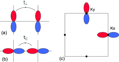
Figure 1: (Color online) The bonding pattern of p-orbitals: (a) the $\sigma$-bonding and (b) the $\pi$-bonding. (c) The p-orbital band structure in a square lattice. The band minima are located at $\vec{K}_{X}=(\frac{\pi}{a},0)$ for the $p_{x}$-orbital band, and $\vec{K}_{Y}=(0,\frac{\pi}{a})$ for the $p_{y}$-orbital band, respectively.

This tight-binding model shows that the energy minima are located at half values of the reciprocal lattice vectors Wu ; Wirth as depicted in Fig.1(c), where $\vec{K}_{X}=(\frac{\pi}{a},0)$ and $\vec{K}_{Y}=(0,\frac{\pi}{a})$. The $p$-orbital bosons can condense at either $K_{X}$ or $K_{Y}$ to form a real BEC or both of $K_{X}$ and $K_{Y}$ to form a complex BEC. To describe the phase transitions we write down a Landau-Ginzberg theory. The action with the most general interactions is cast as following

$$\mathcal{Z}= \int D[\phi^{\ast}_{1},\phi_{1},\phi^{\ast}_{2},\phi_{2}]e^{-S[\phi^{\ast}_{1},\phi_{1},\phi^{\ast}_{2},\phi_{2}]},$$ (3)

where

$$S[\phi^{\ast}_{1},\phi_{1},\phi^{\ast}_{2},\phi_{2}]=$$ (4)

$$\int^{\infty}_{-\infty}\frac{d\omega}{2\pi}\int^{\Lambda}_{0}\frac{d^{2}k}{(2\pi)^{2}}\sum_{i=1,2}\phi_{i}^{\ast}(\omega,\vec{k})(-i\omega+\epsilon_{k}-r_{i})\phi_{i}(\omega,\vec{k})$$ (5)

$$+\int_{\omega k}^{\Lambda}\Big{\{}\sum_{i=1,2}g_{i}\phi_{i}^{\ast}(\omega_{4},\vec{k}_{4})\phi_{i}^{\ast}(\omega_{3},\vec{k}_{3})\phi_{i}(\omega_{2},\vec{k}_{2})\phi_{i}(\omega_{1},\vec{k}_{1})$$ (6)

$$+g_{3}\phi_{2}^{\ast}(\omega_{4},\vec{k}_{4})\phi_{1}^{\ast}(\omega_{3},\vec{k}_{3})\phi_{1}(\omega_{2},\vec{k}_{2})\phi_{2}(\omega_{1},\vec{k}_{1})$$ (7)

$$+g_{4}[\phi_{1}^{\ast}(\omega_{4},\vec{k}_{4})\phi_{1}^{\ast}(\omega_{3},\vec{k}_{3})\phi_{2}(\omega_{2},\vec{k}_{2})\phi_{2}(\omega_{1},\vec{k}_{1})+H.C.]\Big{\}},$$ (8)

where $\phi_{1}$ and $\phi_{2}$ describe the condensate order parameters at $K_{X}$ and $K_{Y}$, respectively. Here we used a short-handed notation $\int_{\omega k}^{\Lambda}=\prod^{4}_{i=1}\int^{\infty}_{-\infty}\frac{d\omega_{i}}{2\pi}\int^{\Lambda}_{0}\frac{d^{2}k_{i}}{(2\pi)^{2}}(2\pi)^{2}\delta(\vec{k}_{4}+\vec{k}_{3}-\vec{k}_{2}-\vec{k}_{1})\cdot(2\pi)\delta(\omega_{4}+\omega_{3}-\omega_{2}-\omega_{1})$. A cutoff $\Lambda$ is given to the momentum space since this is a low energy effective theory. Terms with $g_{1}$ and $g_{2}$ are the intra-species interactions of $p_{x}$ and $p_{y}$ orbital bosons. Terms with $g_{3}$ and $g_{4}$ describes the inter-species interactions. The $g_{4}$ term can rise in this high orbital model as an Umklapp scattering process since the momentum transfer is $\pm 2(\vec{K}_{X}-\vec{K}_{Y})$, which equals to the reciprocal lattice vectors Cai ; Wu .

In contrast to the mean-field theory where certain order parameter is presumably defined, the renormalization group analysis treats various instabilities on an equal footing without assuming any specific order parameters. Here we implement momentum-shell renormalization group method to study the running of various parameters. Following the Wilson’s approach Wilson the renormalization group transformation involves three steps: (i) integrating out all momenta between $\Lambda/s$ and $\Lambda$, for tree level analysis just discarding the part of the action in this momentum-shell; (ii) rescaling frequencies and the momenta as $(\omega,k)\rightarrow(s^{[\omega]}\omega,sk)$ so that the cutoff in k is once again at $\pm\Lambda$; and finally (iii) rescaling fields $\phi\rightarrow s^{[\phi]}\phi$ to keep the free-field action $S_{0}$ invariant.

In order to perform the first step of Wilson’s approach in one-loop level, we need to split the fields into “slow modes” $\phi_{i<}(\omega,\vec{k})$ and “fast modes” $\phi_{i>}(\omega,\vec{k})$. Then we have

$$\phi_{i}(\omega,\vec{k})=\phi_{i<}(\omega,\vec{k})+\phi_{i>}(\omega,\vec{k}),$$ (10)

where

$$\phi_{i<}(\omega,\vec{k})~{}~{}~{}~{}\mbox{for}~{}~{}~{}~{}0<|k|<\Lambda/s,$$ (11)

$$\phi_{i>}(\omega,\vec{k})~{}~{}~{}~{}\mbox{for}~{}~{}~{}~{}\Lambda/s<|k|<\Lambda.$$ (12)

The partition function now can be written as

$$\mathcal{Z}=$$ (13)

$$\int D[\phi^{\ast}_{1<},\phi_{1<},\phi^{\ast}_{2<},\phi_{2<}]e^{-S[\phi^{\ast}_{1<},\phi_{1<},\phi^{\ast}_{2<},\phi_{2<}]}$$ (14)

$$\times\int D[\phi^{\ast}_{1>},\phi_{1>},\phi^{\ast}_{2>},\phi_{2>}]$$ (15)

$$e^{-S_{0}[\phi^{\ast}_{1>},\phi_{1>},\phi^{\ast}_{2>},\phi_{2>}]-S_{I}[\phi^{\ast}_{1<},\phi_{1<},\phi^{\ast}_{2<},\phi_{2<},\phi^{\ast}_{1>},\phi_{1>},\phi^{\ast}_{2>},\phi_{2>}]}.$$ (16)

We next construct an effective action by integration over the fast fields. To the one-loop order, one obtains

$$e^{-S_{eff}[\phi^{\ast}_{1<},\phi_{1<},\phi^{\ast}_{2<},\phi_{2<}]}$$ (18)

$$=e^{-S[\phi^{\ast}_{1<},\phi_{1<},\phi^{\ast}_{2<},\phi_{2<}]}$$ (19)

$$\cdot\exp\Big{[}-\big{<}S_{I}[\phi^{\ast}_{1<},\phi_{1<},\phi^{\ast}_{2<},\phi_{2<},\phi^{\ast}_{1>},\phi_{1>},\phi^{\ast}_{2>},\phi_{2>}]\big{>}_{>}$$ (20)

$$+\frac{1}{2}\big{<}S_{I}[\phi^{\ast}_{1<},\phi_{1<},\phi^{\ast}_{2<},\phi_{2<},\phi^{\ast}_{1>},\phi_{1>},\phi^{\ast}_{2>},\phi_{2>}]^{2}\big{>}_{>}\Big{]},$$ (21)

where $\big{<}...\big{>}_{>}$ denotes the average over the fast fluctuations. we perform the integrals over the fast modes by evaluating the appropriate Feynman diagrams contributing to the renormalization of the vertices of interest. The one-loop Feynman graphs contributing to the renormalization are shown in Fig. 2.

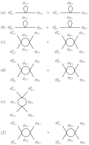
Figure 2: The one-loop Feynman graphs contributing to the renormalization of (a) the parameter $r_{1}$, (b) the parameter $r_{2}$, (c) the interaction $g_{1}$, (d) the interaction $g_{2}$, (e) the interaction $g_{3}$ and (f) the interaction $g_{4}$.

One finds that the parameters $r_{1}$ and $r_{2}$ scale according to the following relations up to one-loop order:

$$\frac{d\tilde{r}_{1}}{d\ell}=2\tilde{r}_{1}+4\tilde{g}_{1}\cdot\theta(\tilde{r}_{1}-1/2)+\tilde{g}_{3}\cdot\theta(\tilde{r}_{2}-1/2),$$ (22)

$$\frac{d\tilde{r}_{2}}{d\ell}=2\tilde{r}_{2}+4\tilde{g}_{2}\cdot\theta(\tilde{r}_{2}-1/2)+\tilde{g}_{3}\cdot\theta(\tilde{r}_{1}-1/2).$$ (23)

In above equations we defined the dimensionless parameters as $\tilde{r}_{i}=r_{i}m/\Lambda^{2}$ and $\tilde{g}_{i}=g_{i}m/(2\pi)$. The $\theta$ functions in the flow equations of $\tilde{r}_{1}$ and $\tilde{r}_{2}$ are from $\omega$ integrations in the one-loop calculations, where we have $\theta(\tilde{r}-1/2)=\int^{+\infty}_{-\infty}\frac{d\omega}{2\pi}\frac{e^{i\omega 0^{+}}}{i\omega-(1/2-\tilde{r})}$. Notice that we introduced the factor $e^{i\omega 0^{+}}$ into the $\omega$ integral otherwise the integral over $\omega$ doesn’t converge Shankar . Most of the studies investigated the behaviors around the critical point, then these contributions can be ignored at zero temperature Sachdev ; Dunkel . However, in our case the running behaviors of $r_{1}$ and $r_{2}$ to $+\infty$ or $-\infty$ are used as the criteria of which phase the system will fall into. Therefore, we have to take these contributions into account. They will give severe influence to the running of $\tilde{r}_{1}$ and $\tilde{r}_{2}$. The flow equations of the coupling constants are as following:

$$\frac{d\tilde{g}_{1}}{d\ell}=-2\tilde{g}^{2}_{1}-2\tilde{g}_{4}^{2},$$ (24)

$$\frac{d\tilde{g}_{2}}{d\ell}=-2\tilde{g}^{2}_{2}-2\tilde{g}_{4}^{2},$$ (25)

$$\frac{d\tilde{g}_{3}}{d\ell}=-\tilde{g}_{3}^{2},$$ (26)

$$\frac{d\tilde{g}_{4}}{d\ell}=-2\tilde{g}_{1}\tilde{g}_{4}-2\tilde{g}_{2}\tilde{g}_{4}.$$ (27)

All the coupling constants with positive initial values are marginally irrelevant. For example, $\tilde{g}_{3}$ can be solved as $\tilde{g}_{3}(\ell)=\frac{\tilde{g}_{3}(0)}{1+\tilde{g}_{3}(0)\ell}$. It approaches to zero as the length scale $\ell$ goes to infinity. However, it doesn’t imply that we can ignore these irrelevant coupling constants. This is because the small $\tilde{g}_{i}$ will generate small contributions to $\tilde{r}_{i}$, which will then quickly grow under the renormalization. As discussed by R. Shankar Shankar , an irrelevant operator can modify the flow of the relevant couplings before it renormalizes to zero.

The running parameters $\tilde{r}_{1}(\ell)$ and $\tilde{r}_{2}(\ell)$ are relevant and can be solved numerically from Eq.(23). We find that in regions of $\tilde{r}_{1}(0)\geq\frac{1}{2}~{}\&~{}\tilde{r}_{2}(0)\geq\frac{1}{2}$ the solutions are

$$\tilde{r}_{1}(\ell)=e^{2\ell}\big{[}\tilde{r}_{1}(0)+\int^{\ell}_{0}e^{-2t}(4\tilde{g}_{1}(t)+\tilde{g}_{3}(t))dt\big{]},$$ (28)

$$\tilde{r}_{2}(\ell)=e^{2\ell}\big{[}\tilde{r}_{2}(0)+\int^{\ell}_{0}e^{-2t}(4\tilde{g}_{2}(t)+\tilde{g}_{3}(t))dt\big{]}.$$ (29)

In this region the initial values $\tilde{r}_{1}(0)$ and $\tilde{r}_{2}(0)$ and the one-loop level contributions are all positive since all the interactions are repulsive. Thus, $\tilde{r}_{1}(\ell)$ and $\tilde{r}_{2}(\ell)$ are both running to positive infinity fast due to the exponential prefactor. The one-loop contributions don’t change the flow directions of the chemical potentials. The running directions of $\tilde{r}_{1}(\ell)$ and $\tilde{r}_{2}(\ell)$ are completely determined by their initial values. If the initial values are positive or negative, they finally flow to positive or negative infinity. In region of $\tilde{r}_{1}(0)\geq\frac{1}{2}~{}\&~{}\tilde{r}_{2}(0)<\frac{1}{2}$ the solutions are

$$\tilde{r}_{1}(\ell)=e^{2\ell}\big{[}\tilde{r}_{1}(0)+\int^{\ell}_{0}e^{-2t}4\tilde{g}_{1}(t)dt\big{]},$$ (30)

$$\tilde{r}_{2}(\ell)=e^{2\ell}\big{[}\tilde{r}_{2}(0)+\int^{\ell}_{0}e^{-2t}\tilde{g}_{3}(t)dt\big{]}.$$ (31)

In region of $\tilde{r}_{1}(0)<\frac{1}{2}~{}\&~{}\tilde{r}_{2}(0)\geq\frac{1}{2}$ the solutions are

$$\tilde{r}_{1}(\ell)=e^{2\ell}\big{[}\tilde{r}_{1}(0)+\int^{\ell}_{0}e^{-2t}\tilde{g}_{3}(t)dt\big{]},$$ (32)

$$\tilde{r}_{2}(\ell)=e^{2\ell}\big{[}\tilde{r}_{2}(0)+\int^{\ell}_{0}e^{-2t}4\tilde{g}_{2}(t)dt\big{]}.$$ (33)

Different from the first region, in these two regions $\tilde{r}_{1}(0)$ or $\tilde{r}_{2}(0)$ can be negative. The positive contributions from the one-loop graphs may qualitatively change the running behaviors of $\tilde{r}_{1}(\ell)$ or $\tilde{r}_{2}(\ell)$. That is, even if $\tilde{r}_{1}(\ell)$ or $\tilde{r}_{2}(\ell)$ runs to negative infinity at the tree level, the positive one-loop contributions can make $\tilde{r}_{1}(\ell)$ or $\tilde{r}_{2}(\ell)$ go to positive infinity eventually. The system will finally end up in a different phase. This generate critical lines these two regions, which are determined by conditions $\tilde{\mu}_{2}(0)+\int^{\infty}_{0}e^{-2t}\frac{\tilde{g}_{3}(0)}{1+\tilde{g}_{3}(0)t}dt=0$ and $\tilde{\mu}_{1}(0)+\int^{\infty}_{0}e^{-2t}\frac{\tilde{g}_{3}(0)}{1+\tilde{g}_{3}(0)t}dt=0.$ However, in other regions the running directions of $\tilde{r}_{1}(\ell)$ and $\tilde{r}_{2}(\ell)$ can eventually be changed by the one-loop corrections from the interaction couplings, even if they renormalize to zero. For instance, in Fig. 3 we start the running of $\tilde{r}_{1}(\ell)$ from a negative initial value.

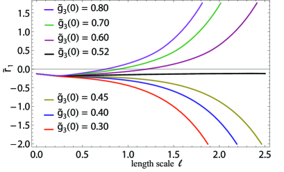
Figure 3: (Color online) The flow directions of parameter $\tilde{r}_{1}(\ell)$ with different interaction coupling $\tilde{g}_{3}(0)$. As $\tilde{g}_{3}(0)$ is increased the running direction of $\tilde{r}_{1}(\ell)$ changes from negative infinity to positive infinity. The system can finally flow to a condensed phase. The initial values of the parameters are $\tilde{r}_{1}(0)=-0.125$, $\tilde{r}_{2}(0)=0.3$ and $\tilde{g}_{1}(0)=\tilde{g}_{2}(0)=\tilde{g}_{4}(0)=0.1$.

As we vary the interaction coupling $\tilde{g}_{3}(0)$ from $0.3$ to $0.8$ we observe that the running of $\tilde{r}_{1}(\ell)$ can finally be changed from the negative to the positive direction. That is, even if $\tilde{r}_{1}(\ell)$ runs to negative infinity at the tree level, the positive one-loop contributions can make $\tilde{r}_{1}(\ell)$ go to positive infinity eventually. The system will finally end up in a different phase. In region of $\tilde{r}_{1}(0)<\frac{1}{2}~{}\&~{}\tilde{r}_{2}(0)<\frac{1}{2}$ the solutions are

$$\tilde{r}_{1}(\ell)=\tilde{r}_{1}(0)e^{2\ell},~{}~{}~{}~{}~{}~{}~{}~{}~{}~{}~{}\tilde{r}_{2}(\ell)=\tilde{r}_{2}(0)e^{2\ell}.$$ (34)

In this region it’s easy to see the running behaviors are totally determined by the tree level scaling. However, with certain initial values $\tilde{r}_{1}(\ell)$ and $\tilde{r}_{2}(\ell)$ can finally flow to the second or the third region and then continuously flow to positive infinity or negative infinity, there are also critical lines in this region.

Based on the numerical calculations the phase diagrams can be drawn in Fig. 4. The four phases are determined by the flow directions of $\tilde{r}_{1}(\ell)$ and $\tilde{r}_{2}(\ell)$ as $\ell\rightarrow\infty$.

• Complex BEC: $\tilde{r}_{1}(\ell)\rightarrow+\infty$ and $\tilde{r}_{2}(\ell)\rightarrow+\infty$,

• Real BEC 1 : $\tilde{r}_{1}(\ell)\rightarrow+\infty$ and $\tilde{r}_{2}(\ell)\rightarrow-\infty$,

• Real BEC 2: $\tilde{r}_{1}(\ell)\rightarrow-\infty$ and $\tilde{r}_{2}(\ell)\rightarrow+\infty$,

• No BEC: $\tilde{r}_{1}(\ell)\rightarrow-\infty$ and $\tilde{r}_{2}(\ell)\rightarrow-\infty$.

We find that without inter-species interactions the complex BEC phase is confined in the first quadrant of the phase diagram as shown in (a) of Fig. 4. However, as we turn on the inter-species interactions the complex phase is enlarged into the second and fourth quadrants as shown in (b), (c) and (d) of Fig. 4.

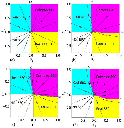
Figure 4: (Color online) Phase diagrams of the $p$-orbital boson system. Four phases are determined by the flow directions of the parameters $\tilde{r}_{1}$ and $\tilde{r}_{2}$ under the renormalization group transformation. In the complex BEC phase $\tilde{r}_{1}(\ell)$ and $\tilde{r}_{2}(\ell)$ run to positive infinities, which represents that both $p_{x}$ and $p_{y}$ orbital bosons condense. In the real BEC 1 (or 2) phase the $p_{x}$ (or $p_{y}$) orbital boson condenses and the other one doesn’t. In the no BEC phase neither of the two orbital bosons condense. The initial values of the couplings are $\tilde{g}_{1}(0)=\tilde{g}_{2}(0)=\tilde{g}_{4}(0)=0.1$ for all of the four diagrams. The inter-species interaction coupling $\tilde{g}_{3}(0)$ between the $p_{x}$ and $p_{y}$ orbital bosons is set to $0,0.1,0.3$ and $0.5$ for graphs (a), (b), (c) and (d) respectively. “b1” and “b2” denote boundary 1 and boundary 2 between the real and complex BEC phases.

Comparing the four phase diagrams in Fig. 4, we see that as the inter-species interaction $\tilde{g}_{3}(0)$ becomes stronger the complex BEC phase get enhanced. That is, certain region of real BEC phases become unstable when the inter-species interactions are turned on and the system finally flows to the complex BEC phase. These interactions give rise to an instability from the real BEC phase to the complex BEC phase. The phase transitions for the real BEC phases to the complex BEC phase require the $U(1)$ symmetry breaking of $p_{x}$ or $p_{y}$ orbital bosons. Given that $\tilde{g}_{3}(0)$ is small, we can obtain the approximate expressions of the two boundaries. Boundary 1 is

$$\tilde{r}_{2}(0)=-\frac{\tilde{r}_{1}(0)\tilde{g}_{3}(0)}{1-\frac{1}{2}\ln(2\tilde{r}_{1}(0))\cdot\tilde{g}_{3}(0)}~{}\mbox{for}~{}0<\tilde{r}_{1}(0)<\frac{1}{2}$$ (35)

$$\tilde{r}_{2}(0)=-\frac{\tilde{g}_{3}(0)}{2}~{}\mbox{for}~{}\tilde{r}_{1}(0)>\frac{1}{2}.$$ (36)

Boundary 2 is

$$\tilde{r}_{1}(0)=-\frac{\tilde{r}_{2}(0)\tilde{g}_{3}(0)}{1-\frac{1}{2}\ln(2\tilde{r}_{2}(0))\cdot\tilde{g}_{3}(0)}~{}\mbox{for}~{}0<\tilde{r}_{2}(0)<\frac{1}{2}$$ (37)

$$\tilde{r}_{1}(0)=-\frac{\tilde{g}_{3}(0)}{2}~{}\mbox{for}~{}\tilde{r}_{2}(0)>\frac{1}{2}.$$ (38)

They are indicated by “$b1$” and “$b2$” in Fig. 4.

III Quantum fluctuation induced symmetry breaking

The mean-field results of the phase transition was derived by constructing a Ginzburg-Landau theory in Ref. Cai . However, our renormalization group analysis gives some qualitative differences: (I) In the mean-field analysis the boundary conditions between the real and complex BEC phases depend on the self-interaction couplings $g_{1}$ and $g_{2}$. However, these two couplings don’t affect the phase boundaries in our results. The quantum phase transition is purely induced by the inter-species interaction between the $p_{x}$ and $p_{y}$ orbital bosons in RG analysis. (II) At one-loop level the $g_{4}$ term doesn’t give any contributions to the flow equations of parameter $r_{1}$ and $r_{2}$. It can get involved in higher order calculations. For instance, $g_{4}$ term can generate corrections to the boundaries “b1” and “b2” at two-loop level through the sunrise graphs in Fig. 5.

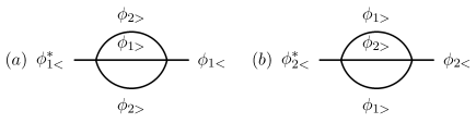
Figure 5: The Feynman diagrams of the two-loop corrections to the parameter (a) $r_{1}$ and (b) $r_{2}$. $\phi_{1}$ and $\phi_{2}$ are the boson fields defined in Eq. (1).

However, in mean-field analysis the phase boundaries depend on both $g_{4}$ and $g_{3}$. This difference originates from the starting points of the two analysis. The $g_{4}$ term explicitly breaks the original $U(1)\times U(1)$ symmetry to $U_{D}(1)$ symmetry, where the index “D” denotes for “Diagonal”, and leads to a fixed phase difference between the two fields $\phi_{1}$ and $\phi_{2}$. The mean-field analysis starts from this symmetry breaking phase. Hence, the complex phase in mean-field is a coherent superposition of the two ground states. However, our renormalization group analysis starts from the normal phase and focuses on the effects of the quantum fluctuations. In this case $g_{4}$ term doesn’t show its contributions up to one-loop level. Our complex phase is just a incoherent mixture of the two ground states. (III) The comparison of the phase diagrams of the renormalization group analysis and mean-field theory can be illustrated in Fig. 6.

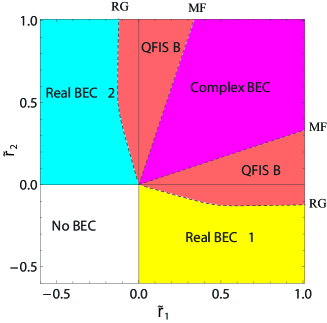
Figure 6: (Color online) Comparison of phase boundaries from the renormalization group analysis and the mean-field analysis. “MF” and “RG” indicate the boundaries from the mean-field and renormalization group analysis respectively. The complex BEC phase in renormalization group analysis is larger than the one from mean-field theory by a region named “QFISB”. The coupling constants are $\tilde{g}_{1}=\tilde{g}_{2}=0.5$, $\tilde{g}_{3}=0.3$ and $\tilde{g}_{4}=0$.

In order to compare the two phase diagrams with the same circumstance we set $g_{4}=0$ in the mean-field phase diagram. The expressions of the mean-field phase boundaries are $\frac{\tilde{r}_{2}}{\tilde{r}_{1}}=\frac{2\tilde{g}_{2}}{\tilde{g}_{3}}$ and $\frac{\tilde{r}_{2}}{\tilde{r}_{1}}=\frac{\tilde{g}_{3}}{2\tilde{g}_{1}}$ Cai . In Fig.6 it’s obvious to see that the crucial difference is that the complex BEC phase is enlarged and the real BEC phase is suppressed in the RG phase diagram.

In essence, the above differences can be explained as effects of the “quantum fluctuation induced symmetry breaking”. The phase transitions from real BEC to complex BEC phase indicate the $U(1)$ symmetry breakdown of field $\phi_{1}$ or $\phi_{2}$. Mean-field description of the symmetry breaking is based on semiclassical approximation. In other words, it’s a tree-level result. When we take into account the quantum fluctuation, the one-loop corrections can significantly change the model parameters and make some region of the real BEC phase become unstable. In Fig. 6 these regions are labeled by “QFISB”. The original QFISB effect was studied using the effective potential method Coleman . Our work reaches a qualitatively analogous result using renormalization group analysis.

Of particular importance is that this phenomenon has qualitative difference from the ordinary quantum corrections to the mean-field results. For instance, in a $s$-orbital system the phase transition is described by $\phi^{4}$ theory. The renormalization group calculations show that the system may flow from a ordered phase to a disordered phase when the quantum fluctuations are taken into account. That is, the quantum fluctuations tend to destroy the ordered phase but not induce it Alexander . However, in our $p$-orbital system the ordered phase of one type of orbital bosons may be induced by the quantum fluctuations from the interactions with the other type of orbital bosons. In Fig. 4 we show that the system in the disordered phase (real BEC phase) may flow to the ordered phase (complex BEC phase) under the RG transformations. Further more, in the $\phi^{4}$ theory of the $s$-orbital system the phase transition occurs at the Wilson-Fisher fixed point with finite values of couplings. The transition is second-order. However, in our work $r_{1}$ and $r_{2}$ are both runaway trajectories. They flow to $+\infty$ or $-\infty$. This infinity is characteristic of first-order phase transition. Actually, the quantum fluctuation induced phase transition has proven to be first-order in effective potential method Amit .

IV Finite temperature scaling and experimental proposal

In order to give a realistic experimental proposal to observe this quantum fluctuation induced first-order phase transition we investigate the finite temperature scaling behaviors of our system. In the vicinity of the quantum critical points the observables obey universal scaling relations. A interesting feature of the scaling approach is that it allows to determine the singular behavior of the physics quantities of interests as a function of temperature at criticality. For instance, we consider the system undergoes a phase transition between the “complex BEC” phase and the “real BEC 2” phase. To discuss this transition, it’s convenient to introduce a parameter $\delta\equiv r_{1}-r_{1c}$ to measure the distance to the transition. Then, the finite temperature scaling behavior of the free energy density near the critical line “b1” can be described as following

$$f(\delta,T)\sim|\delta|^{\nu(d+z)}\tilde{f}(T/|\delta|^{\nu z}),$$ (39)

where $d$ is the special dimension of the system, $\nu$ is the correlation length exponent and $z$ is the dynamic exponent. $\tilde{f}(u)$ is a universal scaling function, which approaches a constant as $u\rightarrow 0$. Thus, the critical temperature $T_{c}$ vanishes like $T_{c}=u_{c}\delta^{z\nu}$ for small $\delta$. A general discussion shows that the scaling behaviors near a first-order phase transition are characterized by the scaling exponents such as $\beta=0$, $\alpha=\gamma=1$ and $\nu=1/(d+z)$ Nienhuis ; Fisher1 . In our case, the dynamic exponent is $z=2$ and the system dimension is $d=2$. Thus, the correlation length exponent is $\nu=1/(d+z)=1/4$. The scaling of the critical temperature is $T_{c}\sim\sqrt{|\delta|}$.

Recently, several schemes were proposed to determine the critical properties in cold-atom systems by extracting the universal scaling functions from the atomic density profiles Zhou ; Hazzard ; Zhang1 . The experimental observations of quantum critical behavior of ultracold atoms have also been reported Donner ; Zhang2 . The study of quantum criticality in cold-atom systems is based on in situ density measurements Zhou ; Hazzard ; Zhang1 ; Zhang2 . The density can be cast as $n(\mu,T)-n_{r}(\mu,T)=T^{\frac{d}{z}+1-\frac{1}{z\nu}}G(\frac{\mu-\mu_{c}}{T^{1/z\nu}})$, where $\mu_{c}$ is the critical value of the chemical potential, $n_{r}$ is the regular part of the density and $G(x)$ is a universal function describing the singular part of the density. Following the scheme developed by Q. Zhou and T.-L. Ho Zhou we can locate the quantum critical point $\mu_{c}$ and then plot the “scaled density” $A(\mu,T)$ versus $(\mu-\mu_{c})/T^{\frac{1}{\nu z}}$, where

$$A(\mu,T)\equiv T^{-\frac{d}{z}-1+\frac{1}{z\nu}}(n(\mu,T)-n_{r}).$$ (40)

The scaled density curves for all temperatures will collapse into a single curve. Then we can utilize this curve of scaling function to test the critical scaling law based on the expected critical exponents.

Within above scheme we consider the observation of the quantum fluctuation induced first-order phase transition in $p$-orbital bosonic system. One leading candidate to observe this phenomenon is ⁸⁷Rb atoms in a bipartite optical square lattice Wirth . The optical potential can be constructed by crossing two laser beams with wavelength $\lambda=1,064$nm and $1/e^{2}$ radius $w_{0}=100r$m. The optical potential reads $-\frac{V_{0}}{4}e^{-\frac{2z^{2}}{w_{0}^{2}}}|\eta[(\hat{z}\cos\alpha+\hat{y}\sin\alpha)e^{ikx}+\epsilon\hat{z}e^{-ikx}]+e^{i\theta}\hat{z}(e^{iky}+\epsilon e^{-iky})|^{2}$. $\epsilon<1$ and $\eta<1$ describe the imperfect reflection and transmission efficiencies, respectively. The typical values of $\epsilon$ and $\eta$ are $\epsilon\approx 0.81$ and $\eta\approx 0.95$. A BEC of $2\times 10^{5}$ ⁸⁷Rb atoms (in the $F=2$, $m_{F}=2$ state) is produced in the optical trap. With $V_{0}$ set to $V_{0}/E_{\mbox{rec}}=6.2$ the excitation of $p$-orbital band can be obtained by ramping $\theta$ from $0.38\pi$ to $0.53\pi$ within 0.2ms. The initial values of the parameter $r_{1}$ and $r_{2}$ can be properly chosen by tuning $\alpha$, which is the angle between the $z$ axis and the linear polarization of the incident beam.

We can fine-tune $\alpha$ to zero so that the system is prepared in the vicinity of the critical line “b1” in Fig. 6. By taking in situ measurement the density profile of the system can be extracted. Following Q. Zhou and T.-L. Ho’s scheme Zhou we can draw a curve of the universal scaling function. If the system undergos a first-order phase transition the scaled density will be in form of $A(\mu,T)=n(\mu,T)-n_{r}$ near the first-order QCP, where we have used $z=2$, $d=2$ and $\nu=\frac{1}{4}$ in Eq. (40). To compare this phase transition with the second-order phase transition we also calculate the scaled density near the second-order QCP, which belongs to the two-dimensional XY universality class with critical exponents $z=2$ and $\nu=1/2$. Then the scaled density is $A(\mu,T)=T^{-1}(n(\mu,T)-n_{r})$. By testing which form the measured scaled density obeys we can determine whether the phase transition is in first or second order.

V Conclusion

In summary, we have investigated the quantum phase transitions of the $p$-orbital boson gas in a square optical lattice using renormalization group method. We find that phase transitions from the real BEC phases to the complex BEC phase can be induced by quantum fluctuations from the interactions between $p_{x}$ and $p_{y}$ orbital bosons. The transition indicates the $U(1)$ symmetry breaking of $p_{x}$ and $p_{y}$ orbital bosons. This is a phenomenon different from the $s$-orbital case, where the quantum fluctuations tend to destroy the ordered phase but not induce it. We find that this effect is purely induced by the inter-species interactions. Our renormalization group analysis also indicates that this is a first-order phase transition. Finally, we gave an experimental proposal to observe this phenomenon in the realistic experiment.

VI Acknowledgements

It’s a pleasure to thank Congjun Wu for suggesting the problem to us. We would also like to thank Jiangping Hu and Anchun Ji for useful discussions. This work is supported by the NKBRSFC under grants Nos. 2012CB821400, 2011CB921502 and 2012CB821305 and NSFC under grants Nos. 1190024, 61227902 and 61378017.

References

- (1) D. Jaksch, C. Bruder, J.I. Cirac, C. W. Gardiner, and P. Zoller, Phys. Rev. Lett. 81, 3108 (1998).
- (2) M. Greiner, O. Mandel, T. Esslinger, T. W. Hänsch, and I. Bloch, Nature 415, 39 (2002).
- (3) T. Müller, S. Fölling, A. Widera, and I. Bloch, Phys. Rev. Lett. 99, 200405 (2007).
- (4) G. Wirth, M. Ölschläger, and A. Hemmerich, Nature Phys. 7, 147 (2011).
- (5) P. Soltan-Panahi, D. Lühmann, J. Struck, P. Windpassinger, and K. Sengstock, Nature Phys. 8, 71 (2012).
- (6) R. P. Feynman, Statistical Mechanics, A Set of Lectures (Addison-Wesley Publishing Company, Boston, Massachusetts, 1972).
- (7) C. Wu, Mod. Phys. Lett. B 23, 1 (2009).
- (8) A. Isacsson and S. M. Girvin, Phys. Rev. A 72, 053604 (2005).
- (9) C. Xu and M. P. A. Fisher, Phys. Rev. B 75, 104428 (2007).
- (10) W. V. Liu and C. Wu, Phys. Rev. A 74, 013607 (2006).
- (11) C. Wu, W. V. Liu, J. E. Moore, and S. Das Sarma, Phys. Rev. Lett. 97, 190406 (2006).
- (12) V. M. Stojanović, C. Wu, W. V. Liu, and S. Das Sarma, Phys. Rev. Lett. 101, 125301 (2008).
- (13) A. B. Kuklov, Phys. Rev. Lett. 97, 110405 (2006).
- (14) Z. Cai and C. Wu, Phys. Rev. A 84, 033635 (2011).
- (15) M. Lewenstein and W. V. Liu, Nature Phys. 7, 101 (2011).
- (16) J. P. Martikainen and J. Larson, Phys. Rev. A 86, 023611 (2012).
- (17) C. Wu, D. Bergman, L. Balents, and S. Das Sarma, Phys. Rev. Lett. 99, 070401 (2007).
- (18) V. W. Scarola and S. Das Sarma, Phys. Rev. Lett. 95, 033003 (2005).
- (19) X. Li, Z. Zhang and W. V. Liu, Phys. Rev. Lett. 108, 175302 (2012).
- (20) C. Wu, Phys. Rev. Lett. 101, 186807 (2008).
- (21) K. Wu and H. Zhai, Phys. Rev. B 77, 174431 (2008).
- (22) E. Zhao and W. V. Liu, Phys. Rev. Lett. 100, 160403 (2008).
- (23) S. Zhang, H. H. Hung, and C. Wu, Phys. Rev. A 82, 053618 (2010).
- (24) X. Li, E. Zhao, and W. V. Liu, Phys. Rev. A 83, 063626 (2011).
- (25) M. Zhang, H. H. Hung, C. Zhang, and C. Wu, Phys. Rev. A 83, 023615 (2011).
- (26) J. Sebby-Strabley, M. Anderlini, P. S. Jessen, and J. V. Porto, Phys. Rev. A 73, 033605 (2006).
- (27) M. Ölschläger, G. Wirth, and A. Hemmerich, Phys. Rev. Lett. 106, 015302 (2011).
- (28) S. Coleman and E. Weinberg, Phys. Rev. D 7, 1888 (1973).
- (29) D. J. Amit, Field Theory, the Renormalization Group and Critical Phenomena (World Scientific, Singapore, 1984).
- (30) B. I. Halperin, T. C. Lubensky, and S. -K. Ma, Phys. Rev. Lett. 32, 292 (1974).
- (31) M. A. Continentino and A. S. Ferreira, Physica A 339, 461 (2004).
- (32) A. S. Ferreira, M. A. Continentino, and E. C. Marino, Phys. Rev. B 70, 174507 (2004).
- (33) Y. Qi and C. Xu, Phys. Rev. B 80, 094402 (2009).
- (34) A. J. Millis, Phys. Rev. B 81, 035117 (2010).
- (35) Jian-Huang She, Jan Zaanen, Alan R. Bishop, and Alexander V. Balatsky, Phys. Rev. B 82, 165128 (2010).
- (36) S. Diehl, M. Baranov, A. J. Daley, and P. Zoller, Phys. Rev. Lett. 104, 165301 (2010).
- (37) Lars Bonnes and Stefan Wessel, Phys. Rev. Lett. 106, 185302 (2011).
- (38) B. Nienhuis and N. Nauenberg, Phys. Rev. Lett. 35, 477 (1975).
- (39) M. E. Fisher and A. N. Berker, Phys. Rev. B 26, 2507 (1982).
- (40) Q. Zhou and T.-L. Ho, Phys. Rev. Lett. 105, 245702 (2010).
- (41) K. R. A. Hazzard and E. J. Mueller, Phys. Rev. A 84, 013604 (2011).
- (42) X. Zhang, C.-L. Hung, S.-K. Tung, N. Gemelke, and C. Chin, New J. Phys. 13, 045011 (2011).
- (43) T. Donner, S. Ritter, T. Bourdel, A. Öttl, M. Köhl, and T. Esslinger, Science 315, 1556 (2007).
- (44) X. Zhang, C.-L. Hung, S.-K. Tung, and C. Chin, Science 335, 1070 (2012).
- (45) K. G. Wilson and J. B. Kogut, Phys. Rep. 12, 75 (1974).
- (46) R. Shankar, Rev. Mod. Phys. 66, 129 (1994).
- (47) S. Sachdev, T. Senthil, and R. Shankar, Phys. Rev. B 50, 258 (1994).
- (48) S. Sachdev and E. R. Dunkel, Phys. Rev. B 73, 085116 (2006).
- (49) A. Altland and B. Simons, Condensed Matter Field Theory (Cambridge University Press, Cambridge, England, 2010).