Nonclassical States of Light and Mechanics

Abstract

This chapter reports on theoretical protocols for generating nonclassical states of light and mechanics. Nonclassical states are understood as squeezed states, entangled states or states with negative Wigner function, and the nonclassicality can refer either to light, to mechanics, or to both, light and mechanics. In all protocols nonclassicallity arises from a strong optomechanical coupling. Some protocols rely in addition on homodyne detection or photon counting of light.

1 Introduction

An outstanding goal in the field of optomechanics is to go beyond the regime of classical physics, and to generate nonclassical states, either in light, the mechanical oscillator, or involving both systems, mechanics and light. The states in which light and mechanical oscillators are found naturally are those with Gaussian statistics with respect to measurements of position and momentum (or field quadratures in the case of light). The class of Gaussian states include for example thermal states of the mechanical mode, as well as its ground state, and on the side of light coherent states and vacuum. These are the sort of classical states in which optomechanical systems can be prepared easily. In this chapter we summarize and review means to go beyond this class of states, and to prepare nonclassical states of optomechanical systems.

Within the family of Gaussian states those states are usually referred to as nonclassical in which the variance of at least one of the canonical variables is reduced below the noise level of zero point fluctuations. In the case of a single mode, e.g. light or mechanics, these are squeezed states. If we are concerned with a system comprised of several modes, e.g. light and mechanics or two mechanical modes, the noise reduction can also pertain to a variance of a generalized canonical variable involving dynamical degrees of freedom of more than one mode. Squeezing of such a collective variable can arise in a state bearing sufficiently strong correlations among its constituent systems. For Gaussian states it is in fact true that this sort of squeezing provides a necessary and sufficient condition for the two systems to be in an inseparable, quantum mechanically entangled state. Nonclassicality within the domain of Gaussian states thus means to prepare squeezed or entangled states.

For states exhibiting non Gaussian statistics the notion of nonclassicality is less clear. One generally accepted criterium is based on the Wigner phase space distribution. A state is thereby classified as non classical when its Wigner function is non positive. This notion of nonclassicality in fact implies for pure quantum states that all non Gaussian states are also non classical since every pure non Gaussian quantum state has a non positive Wigner function. For mixed states the same is not true. Under realistic conditions the state of optomechanical systems will necessarily be a statistical mixture such that the preparation and verification of states with a non positive Wigner distribution poses a formidable challenge. Paradigmatic states of this kind will be states which are close to eigenenergy (Fock) states of the mechanical system.

Optomechanical systems present a promising and versatile platform for creation and verification of either sort of nonclassical states. Squeezed and entangled Gaussian states are in principle achievable with the strong, linearized form of the radiation pressure interaction, or might be conditionally prepared and verified by means of homodyne detection of light. These are all “Gaussian tools” which conserve the Gaussian character of the overall state, but are sufficient to steer the system towards Gaussian non classical states. In order to prepare non Gaussian states, possibly with negative Wigner function, the toolbox has to be enlarged in order to encompass also some non Gaussian instrument. This can be achieved either by driving the optomechanical system with a non Gaussian state of light, such as a single photon state, or by preparing states conditioned on a photon counting event. Ultimately the radiation pressure interaction itself is a nonlinear interaction (cubic in annihilation/creation operators) and therefore does in principle generate non Gausssian states for sufficiently strong coupling $g_{0}$ at the single photon level. Quite generally one can state that some sort of strong coupling condition has to be fulfilled in any protocol for achieving a nonclassical state. Fulfilling the respective strong coupling condition is thus the experimental challenge on the route towards nonclassicality in optomechanics.

In the following we will present a selection of strategies aiming at the preparation of nonclassical states. In Sec. 2 we review ideas of using an optomechanical cavity as source of squeezed and entangled light. Central to this approach is the fact that the radiation pressure provides an effective Kerr nonlinearity for the cavity, which is well known to be able to generate squeezing of light. In Sec. 3 we discuss nonclassical states of the mechanical mode. This involves e.g. the preparation of squeezed states as well as non Gaussian states via state transfer form light, continuous measurement in a nonlinearly coupled optomechanical system, or interaction with single photons and photon counting. Sec. 4 is devoted to nonclassical states involving both systems, light and mechanics, and summarizes ideas to prepare the optomechanical system in an entangled states, either in steady state under continuous wave driving fields, or via interaction with pulsed light.

2 Non-classical states of light

2.1 Ponderomotive squeezing

One of the first predictions of quantum effects in cavity optomechanical system concerned ponderomotive squeezing Mancini1994 ; Fabre1994 , i.e., the possibility to generate quadrature-squeezed light at the cavity output due to the radiation pressure interaction of the cavity mode with a vibrating resonator. The mechanical element is shifted proportionally to the intracavity intensity, and consequently the optical path inside the cavity depends upon such intensity. Therefore the optomechanical system behaves similarly to a cavity filled with a nonlinear Kerr medium. This can be seen also by inserting the formal solution of the time evolution of the mechanical displacement $\hat{x}(t)$ into the Quantum Langevin equation (QLE) for the cavity field annihilation operator $\hat{a}(t)$,

$$\dot{\hat{a}}=-\left[\frac{\kappa}{2}+i\omega_{{\rm opt}}(0)\right]\hat{a}+\int_{-\infty}^{t}ds\chi_{M}(t-s)\left[i\hbar G^{2}\hat{a}(t)\hat{a}^{\dagger}(s)\hat{a}(s)+iG\hat{a}(t)\xi(s)\right]+\sqrt{\kappa}a_{in}(t),$$ (1)

where $a_{in}(t)$ is the driving field (including the vacuum field) and

$$\chi_{M}(t)=\int_{-\infty}^{\infty}\frac{d\omega}{2\pi}\frac{e^{-i\omega t}}{m_{{\rm eff}}\left(\Omega_{{\rm M}}^{2}-\omega^{2}-i\Gamma_{{\rm M}}\omega\right)}=\frac{e^{-\Gamma_{{\rm M}}t/2}}{m_{{\rm eff}}\tilde{\Omega}_{M}}\sin\tilde{\Omega}_{M}t$$ (2)

is the mechanical susceptibility (here $\tilde{\Omega}_{M}=\sqrt{\Omega_{{\rm M}}^{2}-\Gamma_{{\rm M}}^{2}/4}$). Eq. (1) shows that the optomechanical coupling acts as a Kerr nonlinearity on the cavity field, but with two important differences: i) the effective nonlinearity is delayed by a time depending upon the dynamics of the mechanical element; ii) the optomechanical interaction transmits mechanical thermal noise $\xi(t)$ to the cavity field, causing fluctuations of its frequency. When the mechanical oscillator is fast enough, i.e., we look at low frequencies $\omega\ll\Omega_{{\rm M}}$, the mechanical response is instantaneous, $\chi_{M}(t)\simeq\delta(t)/m_{{\rm eff}}\Omega_{{\rm M}}^{2}$, and the nonlinear term becomes indistinguishable from a Kerr term, with an effective nonlinear coefficient $\chi^{(3)}=\hbar G^{2}/m_{{\rm eff}}\Omega_{{\rm M}}^{2}$.

It is known that when a cavity containing a Kerr medium is driven by an intense laser, one gets appreciable squeezing in the spectrum of quadrature fluctuations at the cavity output Walls1995 . The above analogy therefore suggests that a strongly driven optomechanical cavity will also be able to produce quadrature squeezing at its output, provided that optomechanical coupling predominates over the detrimental effect of thermal noise Mancini1994 ; Fabre1994 .

We show this fact by starting from the Fourier-transformed linearized QLE for the fluctuations around the classical steady state

$$m_{{\rm eff}}\left(\Omega_{{\rm M}}^{2}-\omega^{2}-i\omega\Gamma_{{\rm M}}\right)x(\omega) = \hbar G\alpha_{s}\delta X(\omega)+\xi(\omega),$$ (3)

$$\left(\frac{\kappa}{2}-i\omega\right)\delta X(\omega) = -\Delta\delta Y(\omega)+\sqrt{\kappa}\delta X^{in}(\omega),$$ (4)

$$\left(\frac{\kappa}{2}-i\omega\right)\delta Y(\omega) = \Delta\delta X(\omega)+G\alpha_{s}x(\omega)+\sqrt{\kappa}\delta Y^{in}(\omega),$$ (5)

where we have chosen the phase reference so that the stationary amplitude of the intracavity field $\alpha_{s}$ is real, $\delta X=\delta\hat{a}+\delta\hat{a}^{\dagger}$ [$\delta Y=-i\left(\delta\hat{a}-\delta\hat{a}^{\dagger}\right)$] is the amplitude (phase) quadrature of the field fluctuations, and $\delta X^{in}$ and $\delta Y^{in}$ are the corresponding quadratures of the vacuum input field. The output quadrature noise spectra are obtained solving Eqs. (3)-(5), and by using input-output relations Walls1995 , the vacuum input noise spectra $S_{X}^{in}(\omega)=S_{Y}^{in}(\omega)=1$, and the fluctuation-dissipation theorem for the thermal spectrum $S_{\xi}(\omega)=\hbar\omega\Gamma_{{\rm M}}m_{{\rm eff}}\coth\left(\hbar\omega/2k_{B}T\right)$.

The output light is squeezed at phase $\phi$ when the corresponding noise spectrum is below the shot-noise limit, $S_{\phi}^{out}(\omega)<1$, where $S_{\phi}^{out}(\omega)=S_{X}^{out}(\omega)\cos^{2}\phi+S_{Y}^{out}(\omega)\sin^{2}\phi+S_{XY}^{out}(\omega)\sin 2\phi$, and the amplitude and phase noise spectra $S_{X}^{out}(\omega)$ and $S_{y}^{out}(\omega)$ satisfy the Heisenberg uncertainty theorem $S_{X}^{out}(\omega)S_{Y}^{out}(\omega)>1+\left[S_{XY}^{out}(\omega)\right]^{2}$ Braginsky1995 . However, rather than looking at the noise spectrum at a fixed phase of the field, one usually performs an optimization and considers, for every frequency $\omega$, the field phase $\phi_{opt}(\omega)$ possessing the minimum noise spectrum, defining in this way the optimal squeezing spectrum,

$$S_{opt}(\omega) = \min_{\phi}S_{\phi}^{out}(\omega)$$ (6)

$$= \frac{2S_{X}^{out}(\omega)S_{Y}^{out}(\omega)-2\left[S_{XY}^{out}(\omega)\right]^{2}}{S_{X}^{out}(\omega)+S_{Y}^{out}(\omega)+\sqrt{\left[S_{X}^{out}(\omega)-S_{Y}^{out}(\omega)\right]^{2}+4\left[S_{XY}^{out}(\omega)\right]^{2}}}.$$

The frequency-dependent optimal phase is correspondingly given by

$$\phi_{opt}(\omega)=\frac{1}{2}\arctan\left[\frac{2S_{XY}^{out}(\omega)}{S_{X}^{out}(\omega)-S_{Y}^{out}(\omega)}\right].$$ (7)

Since there is no benefit for choosing a nonzero detuning, we restrict to the resonant case $\Delta=0$, which is always stable and where expressions are simpler. One gets

$$S_{X}^{out}(\omega) = 1,\;\;\;\;\;\;\;S_{XY}^{out}(\omega)=\frac{\kappa\hbar G^{2}\alpha_{s}^{2}{\rm Re}\left\{\chi_{M}(\omega)\right\}}{\kappa^{2}/4+\omega^{2}},$$ (8)

$$S_{Y}^{out}(\omega) = 1+S_{XY}^{out}(\omega)^{2}+S_{r}(\omega),$$ (9)

where

$$S_{r}(\omega)=\left[\frac{\kappa\hbar G^{2}\alpha_{s}^{2}{\rm Im}\left\{\chi_{M}(\omega)\right\}}{\kappa^{2}/4+\omega^{2}}\right]^{2}+\frac{\kappa\hbar G^{2}\alpha_{s}^{2}{\rm Im}\left\{\chi_{M}(\omega)\right\}}{\kappa^{2}/4+\omega^{2}}\coth\left(\frac{\hbar\omega}{2k_{B}T}\right).$$ (10)

Inserting Eqs. (8)-(9) into Eq. (6) one sees that the strongest squeezing is obtained when the two limits $S_{r}(\omega)\ll 1$ and $\left[S_{XY}^{out}(\omega)\right]^{2}\gg 1$ are simultaneously satisfied. These conditions are already suggested by Eq. (1): $S_{r}(\omega)\ll 1$ means that thermal noise is negligible, which occurs at low temperatures and small mechanical damping ${\rm Im}\left\{\chi_{M}(\omega)\right\}$, i.e., large mechanical quality factor $Q$; $\left[S_{XY}^{out}(\omega)\right]^{2}\gg 1$ means large radiation pressure, achieved at large intracavity field and small mass. Ponderomotive squeezing is therefore attained when

$$\frac{[S_{XY}^{out}(\omega)]^{2}}{S_{r}(\omega)}\sim\frac{P_{{\rm in}}\omega_{L}}{m_{{\rm eff}}c^{2}\Omega_{{\rm M}}^{2}}\frac{\mathcal{F}^{2}Q}{\bar{n}_{{\rm th}}}\gg 1,$$ (11)

and in this ideal limit $S_{opt}(\omega)\simeq\left[S_{XY}^{out}(\omega)\right]^{-2}\to 0$, and $\phi_{opt}(\omega)\simeq-\arctan\left[2/S_{XY}^{out}(\omega)\right]/2\to 0$. Since the field quadrature $\delta X^{out}$ at $\phi=0$ is just at the shot-noise limit (see Eq. (8)), one has that squeezing is achieved only within a narrow interval for the homodyne phase around $\phi_{opt}(\omega)$, of width $\sim 2\left|\phi_{opt}(\omega)\right|\sim\arctan\left|2/S_{XY}^{out}(\omega)\right|$. This extreme phase dependence is a general and well-known property of quantum squeezing, which is due to the Heisenberg principle: the width of the interval of quadrature phases with noise below the shot-noise limit is inversely proportional to the amount of achievable squeezing.

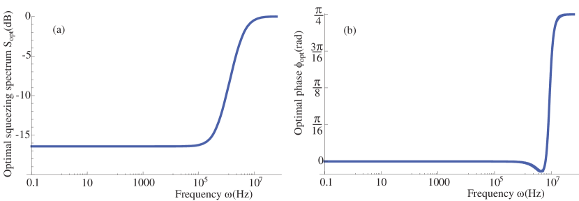
Figure 1: Optimal spectrum of squeezing in dB $S_{opt}$ (a), and the corresponding optimal quadrature phase $\phi_{opt}$ (b), versus frequency in the case of a cavity with bandwidth $\kappa=1$ MHz, length $L=1$ cm, driven by a laser at $1064$ nm and with input power $\mathcal{P}_{in}=10$ mW. The mechanical resonator has $\Omega_{{\rm M}}/2\pi=1$ MHz, mass $m_{{\rm eff}}=100$ ng, quality factor $Q=10^{4}$, and temperature $T=4$ K.

$S_{opt}(\omega)$ and the corresponding optimal phase $\phi_{opt}(\omega)$ at which best squeezing is attained for each $\omega$, are plotted in Fig. 1 for a realistic set of parameter values (see figure caption). $S_{opt}(\omega)$ is below the shot-noise limit whenever $S_{XY}^{out}(\omega)\neq 0$ (see Eqs. (6)-(9)), and one gets significant squeezing at low frequencies, well below the mechanical resonance, where the optomechanical cavity becomes fully equivalent to a Kerr medium, as witnessed also by the fact that $\phi_{opt}(\omega)$ is constant in this frequency band. This equivalence is lost close to and above the mechanical resonance, where squeezing vanishes because ${\rm Re}\left\{\chi_{M}(\omega)\right\}\sim S_{XY}^{out}(\omega)\sim 0$, and the optimal phase shows a large variation.

The present treatment neglects technical limitations: in particular it assumes the ideal situation of a one-sided cavity, where there is no cavity loss because all photons transmitted by the input-output mirror are collected by the output mode. We have also ignored laser phase noise which is typically non-negligible at low frequencies where ponderomotive squeezing is significant. In current experimental schemes both cavity losses and laser phase noise play a relevant role and in fact, ponderomotive squeezing has not been experimentally demonstrated yet. However, the results above show that when these technical limitations will be solved, cavity optomechanical systems may become a valid alternative to traditional sources of squeezing such as parametric amplifiers and Kerr media.

2.2 EPR correlated beams of light

Optomechanical cavities provide a source not only of squeezed light but also of entangled light, as we will explain in the following. By means of spectral filters, the continuous wave field emerging from the cavity can be split in many traveling modes thus offering the option of producing and manipulating a multipartite system Genes2008a . In particular we focus on detecting the first two motional sidebands at frequencies $\omega_{{\rm opt}}\pm\Omega_{{\rm M}}$ and show that they posses quantum correlations of the Einstein-Podolsky-Rosen type Nonclassical:Einstein1935 .

Using the well-known input-output fields connection $\hat{a}^{out}(t)=\sqrt{2\kappa}\hat{a}(t)-\hat{a}^{in}(t)$, the output mode can be split in $N$ independent optical modes by frequency selection with a proper choice of a causal filter function:

$$\hat{a}^{out}_{k}(t)=\int_{-\infty}^{t}dsg_{k}(t-s)\hat{a}^{out}(s),\;\;\;k=1,\ldots N,,$$ (12)

where $g_{k}(s)$ is the causal filter function defining the $k$-th output mode. The annihilation operators describe $N$ independent optical modes when $\left[\hat{a}^{out}_{j}(t),\hat{a}^{out}_{k}(t)^{\dagger}\right]=\delta_{jk}$, which is fulfilled when $\int_{0}^{\infty}dsg_{j}(s)^{*}g_{k}(s)=\delta_{jk}$, i.e., the $N$ filter functions $g_{k}(t)$ form an orthonormal set of square-integrable functions in $[0,\infty)$. As an example of a set of functions that qualify as casual filters we take

$$g_{k}(t)=\frac{\theta(t)-\theta(t-\tau)}{\sqrt{\tau}}e^{-i\Omega_{k}t},$$ (13)

($\theta$ denotes the Heavyside step function) provided that $\Omega_{k}$ and $\tau$ satisfy the condition $\Omega_{j}-\Omega_{k}=\frac{2\pi}{\tau}p$ for integer $p$. Such filtering is seen as a simple frequency integration around $\Omega_{k}$ of bandwidth $\sim 1/\tau$ (the inverse of the time integration window).

For characterization of entanglement one can compute the stationary $(2N+2)\times(2N+2)$ correlation matrix of the output modes defined as

$$V^{out}_{ij}(t)=\frac{1}{2}\left\langle u^{out}_{i}(t)u^{out}_{j}(t)+u^{out}_{j}(t)u^{out}_{i}(t)\right\rangle,$$ (14)

where

$$u^{out}(t)=\left(\hat{q}(t),\hat{p}(t),\hat{X}_{1}^{out}(t),\hat{Y}_{1}^{out}(t),\ldots,\hat{X}_{N}^{out}(t),\hat{Y}_{N}^{out}(t)\right)^{T}$$

is the vector formed by the mechanical position and momentum fluctuations and by the amplitude ($\hat{X}_{k}^{out}(t)=[\hat{a}^{out}_{k}(t)+\hat{a}^{out}_{k}(t)^{\dagger}]/\sqrt{2}$), and phase ($\hat{Y}_{k}^{out}(t)=[\hat{a}^{out}_{k}(t)-\hat{a}^{out}_{k}(t)^{\dagger}]/i\sqrt{2})$ quadratures of the $N$ output modes.

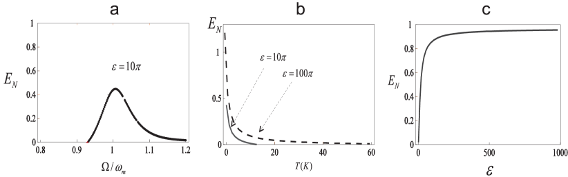
Figure 2: a) Logarithmic negativity of Stoke-Antistokes output modes when $\Omega_{1}=-\Omega_{{\rm M}}$ while $\Omega_{2}$ is varied around $\Omega_{{\rm M}}$. The inverse bandwidth is kept constant at $\epsilon=10\pi$. b) Temperature robustness of bipartite entanglement of output modes at $\pm\Omega_{{\rm M}}$ computed for short ($\epsilon=10\pi$, dashed line) and long ($\epsilon=100\pi$, solid line) detection times. c) The bipartite Stoke-Antistoke entanglement shows improvement and eventually saturates with increasing the integration time. Parameters are $\Omega_{{\rm M}}/2\pi=10$ MHz, $Q=10^{5}$, mass $m_{{\rm eff}}=50$ ng, cavity of length $L=1$ mm with finesse $\mathcal{F}=2\times 10^{4}$, detuning $\Delta=\Omega_{{\rm M}}$, input power $P_{{\rm in}}=30$ mW at $810$ nm, and temperature $T=0.4$ K, yielding $g_{0}=0.43$ kHz, $g=0.41\Omega_{{\rm M}}$, a cavity bandwidth $\kappa=0.75\Omega_{{\rm M}}$, and a thermal occupation of $\bar{n}_{{\rm th}}\simeq 833$.

We are now in position to analyze the quantum correlations between two output modes with the same bandwidth $\tau^{-1}$ and central frequencies $\Omega_{1}$ and $\Omega_{2}$. As a measure for entanglement we apply the logarithmic negativity $E_{\mathcal{N}}$ to the covariance matrix of the two optical modes. It is defined as $E_{\mathcal{N}}=\max[0,-\ln 2\eta^{-}]$, where $\eta^{-}\equiv 2^{-1/2}\left[\Sigma(V)-\left[\Sigma(V)^{2}-4\det V\right]^{1/2}\right]^{1/2}$, with $\Sigma(V)\equiv\det V_{m}+\det V_{c}-2\det V_{mc}$, and we have used the $2\times 2$ block form of the covariance matrix

$$V\equiv\left(\begin{array}[]{cc}V_{m}&V_{mc}\\ V_{mc}^{T}&V_{c}\end{array}\right).$$ (15)

Therefore, a Gaussian state is entangled if and only if $\eta^{-}<1/2$, which is equivalent to Simon’s necessary and sufficient entanglement non-positive partial transpose criterion for Gaussian states, which can be written as $4\det V<\Sigma-1/4$.

The resulting quantum correlations among the upper and the lower sideband in the continuous wave output field are illustrated in Fig. 2. We plot the interesting and not unexpected behavior of $E_{\mathcal{N}}$ as a function of central detection frequency $\Omega$ in Fig.2a, with the mirror reservoir temperature in Fig.2b and with the scaled time integration window $\epsilon=\Omega_{{\rm M}}\tau$ in Fig.2c. The conclusion of Fig.2a is that indeed scattering off the mirror can produce good Stokes-Antistokes entanglement which can be optimized at the cavity output by properly adjusting the detection window. Moreover, further optimization is possible via an integration time increase as suggested by Fig.2c. The temperature behavior plotted in Fig.2b shows very good robustness of the mirror-scattered entangled beams that suggests this mechanism of producing EPR entangled photons as a possible alternative to parametric oscillators.

3 Non-classical states of mechanics

3.1 State transfer

For a massive macroscopic mechanical resonator, just as in the case of a light field, the signature of quantum can be indicated in a first step by the ability of engineering of a squeezed state. Such a state would also be useful in ultrahigh precision measurements or detection of gravitational waves and has been experimentally proven in only one instance for a nonlinear Duffing resonator Nonclassical:Almog2007 . Numerous proposals exist and can be categorized as i) direct: modulated drive in optomechanical settings with or without feedback loop Nonclassical:Clerk2008 ; Nonclassical:Vitali2002 ; Nonclassical:Woolley2008 ; Nonclassical:Tian2008 , and ii) indirect: mapping a squeezed state of light or atoms onto the resonator, coupling to a cavity with atomic medium within Nonclassical:Ian2008 , coupling to a Cooper pair box Nonclassical:Rabl2004 or a superconducting quantum interference loop Nonclassical:Zhou2006 ; Nonclassical:Zhang2009 . In the following we take the example of state transfer in a pure optomechanical setup where laser cooling of a mirror/membrane via a strong laser is accompanied by squeezing transfer from a squeezed vacuum second input light field Nonclassical:Jahne2009 . While the concept is straightforward it is of interest to answer a few practical questions such as: i) what is the resonance condition for optimal squeezing transfer and how does a frequency mismatch affect the squeezing transfer efficiency, ii) what is the optimal transfer, iii) how large should the cavity finesse should be for optimal transfer etc.

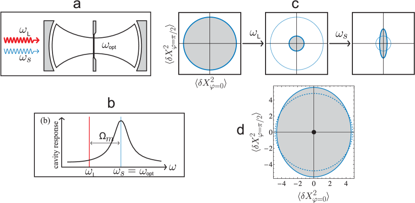
Figure 3: a) Logarithmic negativity of Stoke-Antistokes output modes when $\Omega_{1}=-\Omega_{{\rm M}}$ while $\Omega_{2}$ is varied around $\Omega_{{\rm M}}$. The inverse bandwidth is kept constant at $\epsilon=10\pi$. b) Temperature robustness of bipartite entanglement of output modes at $\pm\Omega_{{\rm M}}$ computed for short ($\epsilon=10\pi$, dashed line) and long ($\epsilon=100\pi$, solid line) detection times. c) The bipartite Stoke-Antistoke entanglement shows improvement and eventually saturates with increasing the integration time.

To this purpose we assume the typical membrane in the middle optomechanical system depicted in Fig. 3a, where the laser Antistokes sideband, the cavity and the squeezing central frequency are resonant (shown in 3b). The input squeezed light operators have the following correlations

$$\langle\hat{c}_{\rm in}(t+\tau)\hat{c}_{\rm in}(t)\rangle=\frac{M}{2}\frac{b_{x}b_{y}}{b_{x}^{2}+b_{y}^{2}}\left(b_{y}e^{-b_{x}|\tau|}+b_{x}e^{-b_{y}|\tau|}\right)$$ (16)

$$\langle\hat{c}^{\dagger}_{\rm in}(t+\tau)\hat{c}_{\rm in}(t)\rangle=\frac{N}{2}\frac{b_{x}b_{y}}{b_{y}^{2}-b_{x}^{2}}\left(b_{y}e^{-b_{x}|\tau|}-b_{x}e^{-b_{y}|\tau|}\right).$$ (17)

The noise operators are written in a frame rotating at $\omega_{\rm s}$ and satisfy the canonical commutation relation $[\hat{c}_{\rm in}(t),\hat{c}^{\dagger}_{\rm in}(t^{\prime})]=\delta(t-t^{\prime})$. Parameters $N$ and $M$ determine the degree of squeezing, while $b_{x}$ and $b_{y}$ define the squeezing bandwidth. For pure squeezing there are only two independent parameters, as in this case $|M|^{2}=N(N+1)$ and $b_{y}=b_{x}\sqrt{2\left(N+|M|\right)+1}$.

Following the standard linearized quantum Langevin equations approach for optomechanics, we first identify two conditions for optimal squeezing: i) $\Delta=\Omega_{{\rm M}}$, meaning that we require continuous laser cooling in the resolved sideband regime and ii) $\Delta_{s}=-\Omega_{{\rm M}}$ so that the squeezing spectrum is centered around the cavity frequency. Then we look at the variances of the generalized quadrature operator

$$\delta\hat{X}_{\varphi}(t) = \frac{1}{\sqrt{2}}\left(e^{i\varphi}\hat{b}(t)+e^{-i\varphi}\hat{b}^{\dagger}(t)\right),$$ (18)

which for $\varphi=0$ is the usual position operator $\hat{q}(t)$ and for $\varphi=-\pi/2$ is the momentum operator $\hat{p}(t)$, both taking in a rotating frame at frequency $\Omega_{{\rm M}}$. In the limit of squeezed white noise the quadrature correlations take a simple form

$$\langle\delta\hat{X}_{\varphi}(t)\delta\hat{X}_{\varphi}(t)\rangle=\left(N+\frac{1}{2}-{\rm Re}\left\{Me^{2i\varphi}\right\}\right)+\frac{\Gamma_{{\rm M}}}{\Gamma_{\rm eff}}\left(\bar{n}_{{\rm th}}+\frac{1}{2}\right).$$ (19)

The first term in the right hand side comes from the squeezing properties of the squeezed input vacuum while the second term is the residual occupancy after laser cooling. In view of this equation a successful squeezed mechanical state preparation automatically requires close to ground state cooling. One can follow this in Fig.3c where cooling close to ground state of an initially thermal mechanical state is performed by the cooling laser, and subsequently squeezing of a quadrature is achieved via the squeezed vacuum. In Fig.3d we suggest that although ground state cooling is not easy to achieve, one can at least in principle (for example by complete tomography of the mechanical state) see a quadrature squashing effect.

To answer a practical question, when the squeezing is not white, fulfilling the resonance condition $\Delta_{s}=-\Omega_{{\rm M}}$ is important. The deviations allowed for the frequency mismatch are smaller than the width of the cooling sideband, i.e. $\Gamma_{\rm eff}$. A second question is the effect of the finite width of squeezing. In general there is an optimal squeezing bandwidth for which the transfer from light to membrane is maximized, but in the resolved sideband limit where $\Omega_{{\rm M}}\gg\kappa$ the finite bandwidth result does not differ much from the infinite bandwidth limit result. For a large bandwidth which fully covers the motional sidebands, $b_{x}\gg\Omega_{{\rm M}}$, the membrane sees only white squeezed input noise, whereas for smaller bandwidth, the crucial question is whether the squeezed input will touch the heating sideband or not. For a high-finesse cavity, the width is not a big issue, since the heating sideband is anyway weak, whereas for a bad cavity the squeezing transfer is much improved for an optimal, finite bandwidth where the strong heating sideband is avoided.

3.2 Continuous measurements of mechanical oscillators.

Another method for creating nonclassical states exploits the possibility to conditionally prepare states of the mechanical oscillator via measuring the output field of the optomechanical system. The coupling of a mechanical resonator to an optical cavity field enables an indirect continuous monitoring of the mechanical motion by a direct phase dependent measurement of the field leaving the cavity. The standard radiation pressure coupling is linear in the displacement of the mechanical resonator and thus enables a continuous measurement of displacement. If we wish to monitor the energy (or phonon number) of the mechanical resonator, however, we need to find an interaction Hamiltonian that is quadratic in the displacement. Such interactions can occur in a number of ways Sankey2010 ; Romero-Isert2011 . We begin with the case of displacement measurements.

The standard linearised opto-mechanical coupling Hamiltonian

$$H=\hbar\Delta\hat{a}^{\dagger}\hat{a}+\hbar\Omega_{{\rm M}}\hat{b}^{\dagger}\hat{b}-\hbar g(\hat{a}+\hat{a}^{\dagger})(\hat{b}+\hat{b}^{\dagger})$$ (20)

As the interaction part of this Hamiltonian commutes with the (dimensionless) mechanical displacement operator, $\hat{q}=\frac{1}{\sqrt{2}}(\hat{b}+\hat{b}^{\dagger})$, in principle this model can be configured as a measurement of the displacement. However as $\hat{q}$ does not commute with the free mechanical Hamiltonian, this is not a strict QND measurement Caves1980 . Nonetheless, for a rapidly damped cavity, we can effect can approximate QND readout of the mechanical displacement provided the coupling constant $g$ can be turned on and off sufficiently fast. This can be achieved by using a pulsed coherent driving field on the cavity Vanner2011 .

If we include the damping of both the cavity and the mechanics, we obtain the quantum stochastic differential equations,

$$\frac{d\hat{a}}{dt} = -i\Delta\hat{a}-\frac{\kappa}{2}\hat{a}+ig\hat{X}+\sqrt{\kappa}\hat{a}_{in}$$ (21)

$$\frac{d\hat{b}}{dt} = -i\Omega_{{\rm M}}\hat{b}-\frac{\Gamma_{{\rm M}}}{2}\hat{b}+ig(\hat{a}+\hat{a}^{\dagger})+\sqrt{\Gamma_{{\rm M}}}\hat{b}_{in}$$ (22)

where we assume that the input noise to the cavity is vacuum, so that the only non zero correlation function for the cavity noise is $\langle\hat{a}_{in}(t)\hat{a}^{\dagger}_{in}(t^{\prime})\rangle=\delta(t-t^{\prime})$ but that the input noise to the mechanical resonator is thermal, $\langle\hat{b}_{in}(t)\hat{b}_{in}^{\dagger}(t^{\prime})\rangle=(\bar{n}_{{\rm th}}+1)\delta(t-t^{\prime})$. We expect that a good measurement will occur when the cavity field is rapidly damped so that it is slaved to the mechanical degree of freedom. We can then adiabatically eliminate the cavity degree of freedom by setting to zero the right hand side of Eq.(21) and formally solving for the operator $\hat{a}$,

$$\hat{a}=\frac{ige^{-i\phi}}{\sqrt{\Delta^{2}+\kappa^{2}/4}}\hat{q}+\frac{\sqrt{\kappa}}{i\Delta+\kappa/2}\hat{a}_{in}$$ (23)

where $\tan\phi=2\Delta/\kappa$. The actual output field from the cavity is related to the field inside by the input/output relation, $\hat{a}_{out}=\sqrt{\kappa}\hat{a}-\hat{a}_{in}$, so that

$$\hat{a}_{out}(t)=\frac{ig\sqrt{\kappa}e^{-i\phi}}{\sqrt{\Delta^{2}+\kappa^{2}/4}}\ \hat{q}(t)+e^{-2i\phi}\hat{a}_{in}(t)$$ (24)

Clearly this indicates that we need to measure a particular quadrature of the output field (for example by homodyne or heterodyne detection) and that the added noise is vacuum noise. The optimal transfer is obtained on resonance. A fast, impulsive readout of the mechanical resonator’s displacement may be made by injecting a coherent pulse into the cavity and subjecting the output pulse to a homodyne measurement Vanner2011 .

If we wish to measure the energy of a mechanical resonator we must find an interaction hamiltonian that is at least quadratic in the mechanical amplitude. A number of schemes have been proposed, including trapped atoms in a standing wave Domokos2003 and a nanomechanical resonator coupled to a single superconducting junction dipole in the dispersive regime Woolley2010 . In opto-mechanics a dielectric membrane placed at the antinode of a cavity standing wave shifts the cavity frequency proportional to the square of the mechanical displacement of the membrane from equilibrium Sankey2010 . A similar interaction arises for an optically levitated particle in a standing wave Romero-Isert2011 .

The interaction Hamiltonian in this case takes the form

$$H=\hbar\omega_{opt}\hat{a}^{\dagger}\hat{a}+\hbar\Omega_{{\rm M}}\hat{b}^{\dagger}\hat{b}+\hbar(\epsilon_{c}^{*}\hat{a}e^{i\omega_{L}t}+\epsilon_{c}\hat{a}^{\dagger}e^{-i\omega_{l}t})+\frac{\hbar}{2}G_{2}\hat{a}^{\dagger}\hat{a}(\hat{b}+\hat{b}^{\dagger})^{2},$$ (25)

where

$$G_{2}=\frac{\hbar}{2\nu m}\left.\frac{\partial^{2}\omega_{c}(x)}{\partial x^{2}}\right|_{x=x_{0}}.$$ (26)

and where we have included a coherent driving field with amplitude $\epsilon$. As usual we expand the interaction around the steady state cavity field. After the rotating wave approximation, the effective Hamiltonian in the interaction picture may then be written as

$$H_{I}=\frac{\hbar}{2}\chi(\bar{\hat{a}}+\bar{\hat{a}}^{\dagger})\hat{b}^{\dagger}\hat{b},$$ (27)

where $\chi=2G_{2}\alpha_{0}$.

The interaction in Eq.(27) describes a displacement of the cavity field proportional to the number of vibrational quanta in the mechanical resonator. The average steady-state displacement is given by $\chi\bar{n}/\kappa$, where $\bar{n}$ is the mean phonon number operator for the mechanical oscillator, $\kappa$ is the cavity line-width. If we continuously monitor the output field amplitude from the cavity via homodyne detection this scheme can in principle enable a continuous monitoring of the mechanical vibrational energy, and phonon number jumps Gangat2011 .

Under continuous homodyne measurement of this quadrature, the system is governed by the following stochastic master equation (SME):

$$d\rho=-\frac{i}{\hbar}[H_{I},\rho]dt+\gamma(\bar{n}_{th}+1)\mathcal{D}[\hat{b}]\rho dt+\gamma\bar{n}_{th}\mathcal{D}[\hat{b}^{\dagger}]\rho dt+\kappa\mathcal{D}[\hat{a}]\rho dt+\sqrt{\kappa}dW\mathcal{H}[ae^{-i\frac{\pi}{2}}]\rho,$$ (28)

where ${\cal D}[c]\rho=c\rho c^{\dagger}-c^{\dagger}c\rho/2-\rho c^{\dagger}c/2$ and $\mathcal{H}[c]\rho=c\rho+\rho c^{\dagger}-$ Tr$(c\rho+\rho c^{\dagger})$ is the measurement super-operator, $\gamma$ and $\kappa$ are the respective mechanical and cavity damping rates.

In figure 4 we show a numerical integration of the stochastic master equation with $\kappa=10^{4}\gamma\bar{N}$ for three cases: $\chi^{2}/\kappa=\gamma\bar{N}$, $\chi^{2}/\kappa=10\gamma\bar{n}_{th}$, and $\chi^{2}/\kappa=10^{2}\gamma\bar{n}_{th}$. We start with the mechanics in the ground state, and the bath temperature is set at $\bar{n}_{th}=0.5$. The first case, Fig. (4a), does not satisfy the fast-measurement condition and therefore does not resolve quantum jumps in the phonon number. The second case, Fig. (4b), is on the border of the fast-measurement regime for $n\sim 1$ and shows some jump-like behaviour in the phonon number. The third case, Fig. (4c), strongly satisfies the fast-measurement condition for low phonon numbers and shows well-resolved quantum jumps in spite of being deeply within the weak coupling regime with $\chi/\kappa=10^{-1}$.

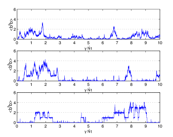
Figure 4: The evolution of the conditional average phonon number with parameters $\kappa=10^{4}\gamma\bar{n}_{th}$ and: (a) $\chi^{2}/\kappa=\gamma\bar{n}_{th}$, (b) $\chi^{2}/\kappa=10\gamma\bar{N}$, (c) $\chi^{2}/\kappa=10^{2}\gamma\bar{n}_{th}$. Jump-like behaviour occurs only when $\chi^{2}/\kappa\gg\gamma[\bar{n}_{th}(n+1)+(\bar{n}_{th}+1)n]$, where $n$ is the phonon number.

For jump-like behaviour to arise in the weak coupling limit, the adiabatic condition is not sufficient. In this regime, analysis shows that the rate of information acquisition about the phonon number is proportional to $\chi^{2}/\kappa$. As in the strong coupling case, this measurement rate must dominate the thermalisation rate in order for quantum jumps to arise. Thus, in addition to being in the adiabatic limit, the weak coupling regime requires $\chi^{2}/\kappa\gg\gamma\bar{N}$.

The state of the mechanical system conditioned on the measurement of light will be in a Non-Gaussian state. This is due to the non-linear interaction introduced in (25). Another way of achieving a Non-Gaussian state exploits the nonlinearity provided in photon counting, as will be detailed in the next section.

3.3 Non-Gaussian state via interaction with single photons and photon counting

In $1935$ Schrödinger pointed out that according to quantum mechanics even macroscopic systems can be in superposition states Schroedinger1935 . The interference effects, characteristic of quantum mechanics, are expected to be hard to detect due to environment induced decoherence decoherence . Nevertheless there have been several proposals on how to create and observe macroscopic superpositions in various physical systems. See references Ruostekoski1998 ; Bose1999 ; Armour2002 for some of the first proposals. There have also been experiments on superposition states in superconducting and piezoelectric devices VanderWaletal2000 ; OConnell2010 and on interference with fullerene Arndt1999 and other large molecules. One long-term motivation for this kind of experiment is the question of whether unconventional decoherence processes such as gravitationally induced decoherence or spontaneous wave-function collapse Ghirardi1986 ; Ghirardi1990 ; Fivel1997 ; Percival1994 ; Penrose2000 take place.

In this section a scheme is analyzed that is close in spirit to Schrödinger’s original discussion. A small quantum system (a photon) is coupled to a large system (a mirror) such that they become entangled Marshall2003 . The system consists of a Michelson interferometer in which one arm has a tiny moveable mirror. The radiation pressure of a single photon is used to displace the tiny mirror. The initial superposition of the photon being in either arm causes the system to evolve into a superposition of states corresponding to two distinct spatial locations of the mirror. A high-finesse cavity is used to enhance the interaction between the single photon and the mirror. The interference of the photon upon exiting the interferometer allows one to study the creation of coherent superposition states periodic with the motion of the mirror.

Consider the setup shown in Fig. 5, consisting of a Michelson interferometer that has a cavity in each arm. In the cavity in arm A one of the mirrors is very small and attached to a micromechanical oscillator. While the photon is inside the cavity, it exerts a radiation pressure force on the small mirror. We will be interested in the regime where the period of the mirror’s motion is much longer than the roundtrip time of the photon inside the cavity, and where the amplitude of the mirror’s motion is very small compared to the cavity length. Under these conditions, the system can be described by the standard optomechanical Hamiltonian Law1993 ; Law1994

$$H=\omega_{{\rm opt}}\hat{a}^{\dagger}\hat{a}+\Omega_{{\rm M}}\hat{b}^{\dagger}\hat{b}-g_{0}\hat{a}^{\dagger}\hat{a}(\hat{b}+\hat{b}^{\dagger}).$$ (29)

To start with, let us suppose that initially the photon is in a superposition of being in either arm $A$ or $B$, and the mirror is in a coherent state $|\beta\rangle=e^{-|\beta|^{2}/2}\sum\limits_{n=0}^{\infty}\frac{\beta^{n}}{\sqrt{n!}}|n\rangle$, where $|n\rangle$ are the eigenstates of the harmonic oscillator. Then the initial state is

$$|\psi(0)\rangle=\frac{1}{\sqrt{2}}(|0\rangle_{A}|1\rangle_{B}+|1\rangle_{A}|0\rangle_{B})|\beta\rangle.$$ (30)

After a time $t$ the state of the system will be given by Mancini1997 ; Bose1997

$$|\psi(t)\rangle =\frac{1}{\sqrt{2}}e^{-i\omega_{{\rm opt}}t}\{|0\rangle_{A}|1\rangle_{B}|\beta e^{-i\Omega_{{\rm M}}t}\rangle$$

$$\quad+e^{i\eta^{2}(\Omega_{{\rm M}}t-\sin\Omega_{{\rm M}}t)}|1\rangle_{A}|0\rangle_{B}|\beta e^{-i\Omega_{{\rm M}}t}+\eta(1-e^{-i\Omega_{{\rm M}}t})\rangle\},$$ (31)

where $\eta=g_{0}/\Omega_{{\rm M}}$. In the second term on the right hand side the motion of the mirror is altered by the radiation pressure of the photon in cavity $A$. The parameter $\eta$ quantifies the displacement of the mirror in units of the size of the coherent state wavepacket. In the presence of the photon the mirror oscillates around a new equilibrium position determined by the driving force.

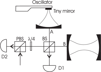
Figure 5: Scheme: a Michelson interferometer for a single photon with in each arm a high-finesse cavity. The cavity in arm A has a very small end mirror mounted on a micro-mechanical oscillator. The single photon enters the interferometer via a polarizing beam splitter (PBS) followed by a $\lambda/4$ wave plate. This is an optical trick to allow detection of the photon leaking out of the interferometer at a later time on detector D1 or D2. If the input photon is considered to be in arm A, the motion of the small mirror is effected by its radiation pressure. If the input photon is considered to be in arm B, the motion of the mirror is undisturbed. The interferometer, based on the 50%/50% beamsplitter (BS), leads to the entanglement between the photon being in arm A or in arm B and the state of the mirror.

The maximum possible interference visibility for the photon is given by twice the modulus of the off-diagonal element of the photon’s reduced density matrix. By tracing over the mirror one finds from Eq. (3.3) that the off-diagonal element has the form

$$\frac{1}{2}e^{-\eta^{2}(1-\cos\Omega_{{\rm M}}t)}e^{i\eta^{2}(\Omega_{{\rm M}}t-\sin\Omega_{{\rm M}}t)+i\eta\mbox{\small Im}[\beta(1-e^{i\Omega_{{\rm M}}t})]}$$ (32)

where Im denotes the imaginary part. The first factor is the modulus, obtaining its minimum value after half a period at $t=\pi/\Omega_{{\rm M}}$, when the mirror is at its maximum displacement. The second factor gives the phase, which is identical to that obtained classically due to the varying length of the cavity.

For general $t$ the phase in Eq. (32) depends on $\beta$, i.e. the initial condition of the mirror. However, the effect of the initial condition averages out after every full period.

In the absence of decoherence, after a full period, $t=2\pi/\Omega_{{\rm M}}$, the system is in the state $\frac{1}{\sqrt{2}}(|0\rangle_{A}|1\rangle_{B}+e^{i\eta^{2}2\pi}|1\rangle_{A}|0\rangle_{B})|\beta\rangle$, such that the mirror is again completely disentangled from the photon. Full interference can be observed if the photon is detected at that moment. If the environment of the mirror “remembers” that the mirror has moved, then, even after a full period, the photon will still be entangled with the mirror’s environment, and thus the interference for the photon will be reduced. Therefore the setup can be used to measure the decoherence of the mirror.

In practice the mirror attached to a mechanical-resonator will be in a thermal state, which can be written as a mixture of coherent states $|\beta\rangle$ with a Gaussian probability distribution $(1/\pi\bar{n}_{{\rm th}})e^{-|\beta|^{2}/\bar{n}_{{\rm th}}}$, where $\bar{n}_{{\rm th}}$ is the mean thermal number of excitations, $\bar{n}_{{\rm th}}=1/(e^{\hbar\Omega_{{\rm M}}/kT}-1)$. If one wants to determine the expected interference visibility of the photon at a time $t$ for an initial mirror state which is thermal, one therefore has to average the off-diagonal element Eq. (32) over $\beta$ with this distribution. The result is

$$\frac{1}{2}e^{-\eta^{2}(2\bar{n}_{{\rm th}}+1)(1-\cos\Omega_{{\rm M}}t)}e^{i\eta^{2}(\Omega_{{\rm M}}t-\sin\Omega_{{\rm M}}t)}.$$ (33)

As a consequence of the averaging of the $\beta$-dependent phase in Eq. (32), the off-diagonal element now decays on a timescale $1/(\eta\Omega_{{\rm M}}\sqrt{\bar{n}_{{\rm th}}})$ after $t=0$, i.e. very fast for the realistic case of large $\bar{n}_{{\rm th}}$. However, remarkably it still exhibits a revival Bose1999 at $t=2\pi/\Omega_{{\rm M}}$, when photon and mirror become disentangled and the phase is independent of $\beta$, such that the phase averaging does not reduce the visibility. Figure 6 shows the time evolution of the visibility of the photon over one period of the mirror’s motion for $\eta=1$ and temperatures $T$ of 1 mK, 100 $\mu$K and 10 $\mu$K.

The magnitude of the revival is reduced by any decoherence of the mirror. Furthermore the revival will also be reduced due to nonlinear terms in the mechanical oscillator. However since we will only consider extremely small displacements around the equilibrium position we assume that nonlinear effects can be ignored.

The revival demonstrates the coherence of the superposition state that exists at intermediate times. For $\eta^{2}\gtrsim 1$ the state of the system is a superposition of two distinct positions of the mirror. More precisely, for a thermal mirror state, the state of the system is a mixture of such superpositions. However, this affects neither the fundamentally non-classical character of the state nor, as we have seen, the existence of the revival after a full period. We now discuss the experimental requirements for achieving such a superposition state and observing its recoherence at $t=2\pi/\Omega_{{\rm M}}$.

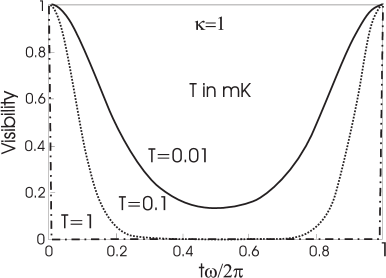
Figure 6: Time evolution of the interference visibility of the photon over one period of the mirror’s motion for $\eta=1$ and temperatures $T$ of 1 mK, 100 $\mu$K and 10 $\mu$K. The visibility decays very fast after $t=0$, but in the absence of decoherence there is a sharp revival of the visibility after a full period (2$\pi$). The width of each peak scales like $1/\sqrt{T}$.

Firstly, it is required that $\eta^{2}\gtrsim 1$, which physically means that the momentum kick imparted by the photon to the mirror has to be larger than the initial quantum momentum uncertainty of the mirror. Let $N$ denote the number of roundtrips of the photon in the cavity during one period of the mirror’s motion, such that $2NL/c=2\pi/\Omega_{{\rm M}}$. This allows us to rewrite the condition $\eta^{2}\gtrsim 1$ as

$$\frac{2\hbar N^{3}L}{\pi cm_{{\rm eff}}\lambda^{2}}\gtrsim 1,$$ (34)

where $\lambda$ is the wavelength of the light. The factors entering Eq. (34) are not all independent. The achievable $N$, which is determined by the quality of the mirrors, and the minimum possible mirror size depend strongly on $\lambda$. The mirror’s lateral dimensions should be an order of magnitude larger than $\lambda$ to limit diffraction and avoid geometrical losses. The minimum possible thickness of the mirror generally depends on the wavelength as well in order to achieve sufficiently low transmission.

Eq. (34) allows one to compare the viability of different wavelength ranges. While the highest values for $N$ are achievable for microwaves (up to $10^{10}$), this is counteracted by their long wavelengths (of order cm). On the other hand there are no good mirrors for highly energetic photons. The optical regime seems optimal. In the following estimates we will consider a $\lambda$ around 630 nm.

The cavity mode needs to have a very narrow focus on the tiny mirror, which requires the other cavity end mirror to be large due to beam divergence. The maximum cavity length is therefore limited by the difficulty of making large high quality curved mirrors. In fact from simulations it follows that indeed the surface quality of the large curved mirror is likely to be the most challenging component of the setup Kleckner2006 ; Kleckner2010 . Here we consider a cavity length of 5 cm, and a small mirror size of 10 x 10 x 10 microns, leading to a mass of order $5\times 10^{-12}$ kg.

One possible path for the fabrication of such a small mirror on a good mechanical oscillator is to coat a silicon cantilever with alternating layers of SiO₂ and a metal oxide such as Ta₂O₅ by sputtering deposition. The best current mirrors are made in this way. Recently such mirrors have also been produce on Silicon Nitride cross resonators which have excellent mechanical properties Kleckner2011 .

For the above dimensions the condition (34) is satisfied for $N=5.6\times 10^{6}$. Therefore a photon loss per reflection not larger than $3\times 10^{-7}$ is needed, which is about a factor of 4 below the best reported values for such mirrors Rempe1992 , and for a transmission of $10^{-7}$, which is consistent with the quoted mirror thickness Hood2001 . For these values, about 1% of the photons are still left in the cavity after a full period of the mirror. Coupling into a high-finesse cavity with a tight focus will require carefully designed incoupling optics. For the above values of $N$ and $L$ one obtains a frequency $\Omega_{{\rm M}}=2\pi\times 500$ Hz. This leads to a quantum uncertainty of order $10^{-13}$ m, which for $\eta^{2}\sim 1$ corresponds to the displacement in the superposition.

Secondly, the requirement of observing the revival after a full period of the mirror’s motion puts a bound on the acceptable environmental decoherence. To estimate the expected decoherence we model the mirror’s environment by an (Ohmic) bath of harmonic oscillators. Applying the analysis of Strunz2002 one then finds that off-diagonal elements between different mirror positions decay with a factor

$$\exp{\left[-\frac{\Gamma_{{\rm M}}kTm_{{\rm eff}}(\Delta x)^{2}}{\hbar^{2}}\left(t+\frac{\sin\Omega_{{\rm M}}t\cos\Omega_{{\rm M}}t}{\Omega_{{\rm M}}}\right)\right]},$$ (35)

where $\Gamma_{{\rm M}}$ is the rate of energy dissipation for the mechanical oscillator, $T$ is the temperature (which is constituted mainly by the internal degrees of freedom of the mirror cantilever) and $\Delta x$ is the separation of two coherent states that are originally in a superposition. Note that our experiment is not in the long-time regime where decoherence is characterized simply by a rate. However, the oscillatory term in the exponent of Eq. (35) does not affect the order of magnitude and happens to be zero after a full period. Assuming that the experiment achieves $\eta^{2}\gtrsim 1$, i.e. a separation by the size of a coherent state wavepacket, $\Delta x=\sqrt{\frac{\hbar}{m_{{\rm eff}}\Omega_{{\rm M}}}}$, the condition that the exponent in Eq. (35) should be at most of order 1 after a full period can be cast in the form

$$Q\gtrsim\frac{kT}{\hbar\Omega_{{\rm M}}}=\bar{n}_{{\rm th}},$$ (36)

where $Q=\Omega_{{\rm M}}/\Gamma_{{\rm M}}$ is the quality factor of the mechanical oscillator. Bearing in mind that quality factors of the order of $10^{5}-10^{6}$ have been achieved for silicon cantilevers of approximately the right dimensions and frequency, this implies that the temperature has to be approximately 3-30 mK. It will be beneficial to perform experiments at even lower temperatures to reduce the measurement time, as we will explain below.

Thirdly, the stability requirements for the experiment are very strict. The phase of the interferometer has to be stable over the whole measurement time. This means that in particular the distance between the large cavity end mirror and the equilibrium position of the small mirror has to be stable to of order $\lambda/20N=0.6\times 10^{-14}$m.

The required measurement time can be determined in the following way. A single run of the experiment starts by sending a weak pulse into the interferometer, such that on average 0.1 photons go into either cavity. This probabilistically prepares a single-photon state as required to a good approximation. The two-photon contribution has to be kept low because it causes noise in the interferometer. From Eq. (33) the width of the revival peak is $2/\eta\Omega_{{\rm M}}\sqrt{\bar{n}_{{\rm th}}}$. This implies that only a fraction $\sim 1/\pi\sqrt{\bar{n}_{{\rm th}}}$ of the remaining photons will leak out in the time interval of the revival. It is therefore important to work at the lowest possible temperature. Temperatures below 100 $\mu$K can be achieved with a nuclear demagnetization cryostat.

Together with the required low value of $\Omega_{{\rm M}}$, the fact that approximately 1% of the photons remain after a full period for our assumed loss, and an assumed detection efficiency of 70 %, this implies a detection rate of approximately 100 photons per hour in the revival interval. This means that a measurement time of order 30 minutes should give convincing statistics.

After every single run of the experiment the mirror has to be damped to reset it to its initial (thermal) state. This could be done by electric or magnetic fields, e.g. following Ref. Wago1998 , where a Nickel sphere was attached to the cantilever, whose $Q$ could then be changed by 3 orders of magnitude by applying a magnetic field.

Since the width of the revival peak scales like $1/\sqrt{T}$, the required measurement time can also be decreased by decreasing the temperature below 60 $\mu$K. Passive cooling techniques may be improved. In addition, active and passive optical cooling of mirror oscillators has been proposed Mancini1998 , and implemented experimentally for a large mirror Cohadon1999 and for small mirrors Kleckner2006a ; Arcizet2006 ; Gigan2006 ; Kippenberg2008 . Ground state cooling of the center of mass motion is achievable and reduces the required measurement time, and thus the stability requirements, by a factor of approximately 50.

4 Entangled states of mechanics and light

In this last section we turn our attention to non-classical states involving both, light and mechanics. In our discussion these will be primarily entangled states, which are generated either in steady state under a continuous drive field, or in a regime involving short pulses of light.

4.1 Light mirror entanglement in steady state

Entanglement of a mechanical oscillator with light has been predicted in a number of theoretical studies Genes2008a ; paternostro_creating_2007 ; miao_universal_2010 ; vitali_optomechanical_2007 ; galve_bringing_2010 ; genes_simultaneous_2008 ; vitali_entangling_2007 ; ghobadi_optomechanical_2011 ; ghobadi_quantum_2011 ; abdi_effect_2011 and would be an intriguing demonstration of optomechanics in the quantum regime. These studies, as well as similar ones investigating entanglement among several mechanical oscillators mancini_entangling_2002 ; zhang_quantum-state_2003 ; pinard_entangling_2005 ; pirandola_macroscopic_2006 ; hartmann_steady_2008 ; vacanti_optomechanical_2008 ; huang_entangling_2009 ; vitali_stationary_2007 ; ludwig_entanglement_2010 , explore entanglement in the steady-state regime. In this regime the optomechanical system is driven by one or more continuous-wave light fields and settles into a stationary state, for which the interplay of optomechanical coupling, cavity decay, damping of the mechanical oscillator, and thermal noise forces may remarkably give rise to persistent entanglement between the intracavity field and the mechanical oscillator.

The simplest example of such a scheme involves an optomechanical system driven by one continuous wave laser field. To identify conditions for good optomechanical generation of entanglement we answer a first question that concerns the optimal detuning of the driving laser with respect to the cavity field. Given the form of the linearized radiation pressure Hamiltonian $\hbar g(\hat{a}+\hat{a}^{{\dagger}})(\hat{b}+\hat{b}^{{\dagger}})$, and the time evolution of operators with frequencies $\Delta$ and $\Omega_{{\rm M}}$, we focus on resonant processes where $\Delta=\pm\Omega_{{\rm M}}$. The first case we analyze is blue-detuning $\Delta=-\Omega_{{\rm M}}$ and in which we split the interaction in two kind of interactions well known in quantum optics: i) beam splitter interaction $\hbar g(\hat{a}^{{\dagger}}\hat{b}+h.c.)$ and ii) down-conversion interaction, $\hbar g(\hat{a}\hat{b}+h.c.)$. Since the beam splitter term is off-resonant by $2\Omega_{{\rm M}}$ and also cannnot produce entanglement starting from classical states we drop it and focus on the down-conversion term, known to produce bipartite entanglement. Following a standard treatment to obtain the covariance matrix in steady state (even analytically for this particular case), it can be shown that the logarithmic negativity scales up with $g$ as

$$E_{\mathcal{N}}\leq\ln\left[\frac{1+g/\sqrt{2\kappa\Gamma_{{\rm M}}}}{1+\bar{n}_{{\rm th}}}\right].$$ (37)

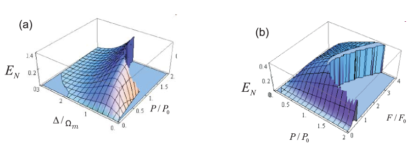
Figure 7: (a) Logarithmic negativity $E_{\mathcal{N}}$ versus the normalized detuning $\Delta/\Omega_{{\rm M}}$ and normalized input power $P_{{\rm in}}/P_{{\rm in}}^{0}$, ($P_{{\rm in}}^{0}=50$ mW) at a fixed value of the cavity finesse $\mathcal{F}=\mathcal{F}_{0}=1.67\times 10^{4}$; (b) $E_{\mathcal{N}}$ versus the normalized finesse $\mathcal{F}/\mathcal{F}_{0}$ and normalized input power $P_{{\rm in}}/P_{{\rm in}}^{0}$ at a fixed detuning $\Delta=\Omega_{{\rm M}}$. Parameter values are $\Omega_{{\rm M}}/2\pi=10$ MHz, $\mathcal{Q}=10^{5}$, mass $m_{{\rm eff}}=10$ ng, a cavity of length $L=1$ mm driven by a laser with wavelength $810$ nm, yielding $g=0.95$ KHz and a cavity bandwidth $\kappa=0.9\Omega_{{\rm M}}$ when $\mathcal{F}=\mathcal{F}_{0}$. We have assumed a reservoir temperature for the mirror $T=0.4$ K, corresponding to $\bar{n}_{{\rm th}}\simeq 833$. The sudden drop to zero of $E_{\mathcal{N}}$ corresponds to entering the instability region.

However, the system is unstable in the ”blue-detuned” regime owing to the fast transfer of energy from the cavity field to the mirror and an unavoidable bound is found $g<\sqrt{(}2\kappa\Gamma_{{\rm M}})$ which in consequence limits $E_{\mathcal{N}}\leq\ln 2$. Moreover, any thermal quantum $\bar{n}_{{\rm th}}>0$ completely destroys the entanglement. One therefore concludes that the choice of the practical operation regime is dictated by the stability of the system. Thus, we move into the ”red detuned” which allows for larger $g$ by paying the price that, for example at $\Delta=\Omega_{{\rm M}}$ the down-convers on process is $2\Omega_{{\rm M}}$ off-resonant. In this regime analytical results are possible but cumbersome and we settled for numerically showing the behavior of $E_{\mathcal{N}}$ in Fig. 7a as it scales with increasing input power and varying detunings, and in 7b with input power and cavity finesse.

Having concluded that intracavity optomechanical entanglement is attainable, the question of detection is to be answered next. As detailed in vitali_optomechanical_2007 a simple scheme can be conceived that consists of a second cavity adjacent to the main one; the second cavity output, when weakly driven, does not modify much the first cavity dynamics and its output light gives a direct measurement of the mirror dynamics. With homodyne detection of both cavities and manipulation of the two local oscillators phases one can determine all of the entries of the covariance matrix and them numerically extract the logarithmic negativity.

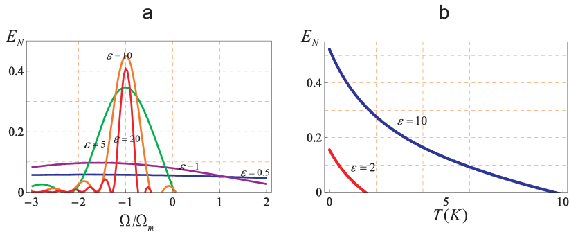
Figure 8: (a) Logarithmic negativity $E_{\mathcal{N}}$ vs. $\Omega/\Omega_{{\rm M}}$ for different values of $\epsilon$. Optimal entanglement of the Stokes sideband with the mirror can be deduced. (b) $E_{\mathcal{N}}$ of output Stokes mode with mirror versus $T$ for two different values of its inverse bandwidth $\epsilon=2,10$.

As previously mentioned, in the ”red-detuning” regime, the down-conversion process is off-resonant and its effect much washed out by the presence of the stronger beam-splitter interaction. However, proper detection around the Stokes sideband (which carries the photons entangled with the mirror) in the sense described in 2.2 can extract optimal light-mirror entanglement Genes2008a . We show this by choosing a central frequency of the detected mode $\Omega$ and its bandwidth $\tau^{-1}$ and computing the bipartite system negativity. The results are shown in Fig. 8a, where $E_{\mathcal{N}}$ is plotted versus $\Omega/\Omega_{{\rm M}}$ at five different values of $\epsilon=\tau\Omega_{{\rm M}}$ and the other parameters similar to the ones used for Fig. 7. If $\epsilon<1$, i.e., the bandwidth of the detected mode is larger than $\Omega_{{\rm M}}$, the detector does not resolve the motional sidebands, and $E_{\mathcal{N}}$ has a value (roughly equal to that of the intracavity case) which does not essentially depend upon the central frequency. For smaller bandwidths (larger $\epsilon$), the sidebands are resolved by the detection and the role of the central frequency becomes important. In particular $E_{\mathcal{N}}$ becomes highly peaked around the Stokes sideband $\Omega=-\Omega_{{\rm M}}$, showing that the optomechanical entanglement generated within the cavity is mostly carried by this lower frequency sideband. What is relevant is that the optomechanical entanglement of the output mode is significantly larger than its intracavity counterpart and achieves its maximum value at the optimal value $\epsilon\simeq 10$, i.e., a detection bandwidth $\tau^{-1}\simeq\Omega_{{\rm M}}/10$. This means that in practice, by appropriately filtering the output light, one realizes an effective entanglement distillation because the selected output mode is more entangled with the mechanical resonator than the intracavity field.

It is finally important to see what the robustness of the entanglement is with increasing temperature of the thermal reservoir. This is shown by Fig. 8b, where the entanglement $E_{\mathcal{N}}$ of the output mode centered at the Stokes sideband is plotted versus the temperature of the reservoir at two different values of the bandwidth, the optimal one $\epsilon=10$, and at a larger bandwidth $\epsilon=2$. We see the expected decay of $E_{\mathcal{N}}$ for increasing temperature, but above all that also this output optomechanical entanglement is robust against temperature because it persists even above liquid He temperatures, at least in the case of the optimal detection bandwidth $\varepsilon=10$.

4.2 Entanglement with pulsed light

An alternative approach to achieving optomechanical entanglement works in a pulsed regime. It does not rely on the existence of a stable steady state, such that entanglement is not limited by stability requirements. In fact it is possible to operate in a parameter regime where a stationary state does not exist. This sort of optomechanical entanglement can be verified by using a pump–probe sequence of light pulses. The quantum state created in this protocol exhibits Einstein–Podolsky–Rosen (EPR) type entanglement Nonclassical:Einstein1935 between the mechanical oscillator and the light pulse. It thus provides the canonical resource for quantum information protocols involving continuous variable (CV) systems braunstein_quantum_2005 . Optomechanical EPR entanglement can therefore be used for the teleportation of the state of a propagating light pulse onto a mechanical oscillator as suggested in mancini_scheme_2003 ; pirandola_continuous-variable_2003 .

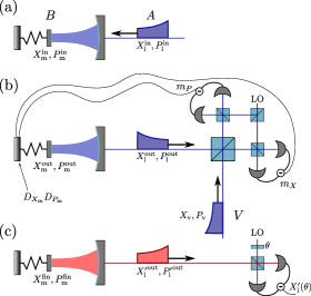
Figure 9: Schematic of the system and the proposed teleportation protocol: (a) A blue detuned light pulse (A) is entangled with the mirror (B). (b) A second light pulse (V) is prepared in the input state and interferes with A on a beam-splitter. Two homodyne detectors measure $P^{\mathrm{out}}_{\mathrm{l}}+X_{\mathrm{v}}$ and $X^{\mathrm{out}}_{\mathrm{l}}+P_{\mathrm{v}}$, yielding outcomes $m_{X}$ and $m_{P}$ respectively. Feedback is applied by displacing the mirror state in phase space by a unitary transformation $D_{X_{\mathrm{m}}}\!(m_{X})\,D_{P_{\mathrm{m}}}\!(m_{P})$. (c) To verify the success of the protocol, the mirror state is coherently transferred to a red detuned laser pulse and a generalised quadrature $X^{\prime}_{\mathrm{l}}(\theta)={X^{\prime}_{\mathrm{l}}}^{\mathrm{out}}\cos\theta+{P_{\mathrm{l}}^{\prime}}^{\mathrm{out}}\sin\theta$ is measured. Repeating steps (a)–(c) for the same input state but for different phases $\theta$ yields a reconstruction of the mirror’s quantum state.

Let us consider an optomechanical cavity in a Fabry–P rot type setup, cf. Fig. 9). A light pulse of duration $\tau$ and carrier frequency $\omega_{\mathrm{l}}$ impinges on the cavity and interacts with the oscillatory mirror mode via radiation pressure. In a frame rotating with the laser frequency, the system is described by the (effective) Hamiltonian Mancini1994

$$H=\Omega_{{\rm M}}\hat{b}^{\dagger}\hat{b}+\Delta\hat{a}^{\dagger}\hat{a}+g\left(\hat{b}+\hat{b}^{\dagger}\right)\left(\hat{a}+\hat{a}^{\dagger}\right)$$ (38)

where $\Delta=\omega_{{\rm opt}}-\omega_{\mathrm{l}}$ is the detuning of the laser drive with respect to the cavity resonance. We assume the pulse to approximately be a flat-top pulse, which has a constant amplitude for the largest part, but possesses a smooth head and tail. The coupling constant $g$ is then given by

$$g=g_{0}\sqrt{\frac{2\kappa N_{\mathrm{ph}}/\tau}{(\Delta^{2}+\kappa^{2})}},$$ (39)

with $N_{\mathrm{ph}}$ the number of photons in the pulse. It is possible to make either the a beam-splitter like interaction ($\hat{a}\hat{b}^{\dagger}+\hat{b}\hat{a}^{\dagger}$) or the two-mode-squeezing interaction ($\hat{a}\hat{b}+\hat{a}^{\dagger}\hat{b}^{\dagger}$) resonant by tuning the laser to one of the motional sidebands $\omega_{{\rm opt}}\pm\Omega_{{\rm M}}$, where the blue (anti-Stokes) sideband ($\omega_{\mathrm{l}}=\omega_{{\rm opt}}+\Omega_{{\rm M}}$) enhances down-conversion, while the red (Stokes) sideband ($\omega_{\mathrm{l}}=\omega_{{\rm opt}}-\Omega_{{\rm M}}$) enhances the beam-splitter interaction Aspelmeyer2010 . In the proposed protocol we make use of both dynamics separately: Pulses tuned to the blue sideband are applied to create entanglement, while pulses on the red sideband are later used to read out the final mirror state. A similar separation of Stokes and anti-Stokes sideband was suggested in mancini_scheme_2003 ; pirandola_continuous-variable_2003 by selecting different angles of reflection of a light pulse scattered from a vibrating mirror in free space.

The full system dynamics, including the dissipative coupling of the mirror and the cavity decay, are described by quantum Langevin equations gardiner_quantum_2004 , which determine the time evolution of the corresponding operators $x_{\mathrm{m}}=(\hat{b}+\hat{b}^{\dagger})/\sqrt{2}$, $p_{\mathrm{m}}=-i(\hat{b}-\hat{b}^{\dagger})/\sqrt{2}$ and $\hat{a},\hat{a}^{\dagger}$. They read

$$\dot{x}_{\mathrm{m}} = \phantom{-}\Omega_{{\rm M}}p_{\mathrm{m}},$$ (40)

$$\dot{p}_{\mathrm{m}} = -\Omega_{{\rm M}}x_{\mathrm{m}}-\Gamma_{{\rm M}}\,p_{\mathrm{m}}-\sqrt{2}\,g\left(\hat{a}+\hat{a}^{\dagger}\right)-\sqrt{2\Gamma_{{\rm M}}}\,f,$$ (41)

$$\dot{a}_{\mathrm{c}} = -(i\Delta+\kappa)\hat{a}-i\sqrt{2}\,g\,x_{\mathrm{m}}-\sqrt{2\kappa}\,a_{in},$$ (42)

where we introduced the (self-adjoint) Brownian stochastic force $f$, and quantum noise $a_{in}$ entering the cavity from the electromagnetic environment. Both $a_{in}$ and—in the high-temperature limit—$f$ are assumed to be Markovian. Their correlation functions are thus given by $\langle{a_{in}(t)a_{in}^{\dagger}(t^{\prime})}\rangle=\delta(t-t^{\prime})$ (in the optical vacuum state) and $\langle f(t)f(t^{\prime})+f(t^{\prime})f(t)\rangle=(2\bar{n}_{{\rm th}}+1)\delta(t-t^{\prime})$ (in a thermal state of the mechanics) gardiner_quantum_2004 .

We impose the following conditions on the system’s parameters. Firstly, we drive the cavity on the blue sideband ($\Delta=-\Omega_{{\rm M}}$) and assume to work in the resolved-sideband regime ($\kappa\ll\Omega_{{\rm M}}$) to enhance the down-conversion dynamics. Note that in this regime a stable steady state only exists for very weak optomechanical coupling ludwig_optomechanical_2008 , which poses a fundamental limit to the amount of entanglement that can be created in a continuous-wave scheme Genes2008a . In contrast, a pulsed scheme does not suffer from these instability issues. In fact, it is easy to check by integrating the full dynamics up to time $\tau$, that working in this particular regime yields maximal entanglement, which increases with increasing sideband-resolution $\Omega_{{\rm M}}/\kappa$. Secondly we assume a weak optomechanical coupling $g\ll\kappa$, such that only first-order interactions of photons with the mechanics contribute. This minimises pulse distortion and simplifies the experimental realization of the protocol. Taken together, the conditions $g\ll\kappa\ll\Omega_{{\rm M}}$ allow us to invoke the rotating-wave-approximation (RWA), which amounts to neglecting the beam-splitter term in 38. Also, we neglect mechanical decoherence effects in this section. We emphasise that this approximation is justified as long as the total duration of the protocol is short compared to the effective mechanical decoherence time $1/\Gamma_{{\rm M}}\bar{n}_{{\rm th}}$, where $\Gamma_{{\rm M}}$ is the mechanical damping rate and $\bar{n}_{{\rm th}}$ the thermal occupation of the corresponding bath. Corrections to this simplified model will be addressed below.

Based on the assumptions above we can now simplify equations 40. For convenience we go into a frame rotating with $\Omega_{{\rm M}}$ by substituting $\hat{a}\rightarrow\hat{a}e^{i\Omega_{{\rm M}}t}$, $a_{in}\rightarrow a_{in}e^{i\Omega_{{\rm M}}t}$ and $\hat{b}\rightarrow\hat{b}e^{-i\Omega_{{\rm M}}t}$. Note that in this picture the central frequency of $a_{in}$ is located at $\omega_{\mathrm{l}}-\Omega_{{\rm M}}=\omega_{{\rm opt}}$. In the RWA the Langevin equations then simplify to

$$\dot{a}_{\mathrm{c}} =-\kappa\hat{a}\,-ig\,\hat{b}^{\dagger}-\sqrt{2\kappa}\,a_{in}, \dot{a}_{\mathrm{m}} =-ig\,\hat{a}^{\dagger}.$$ (43)

In the limit $g\ll\kappa$ we can use an adiabatic solution for the cavity mode and we therefore find

$$\hat{a}(t) \approx-i\frac{g}{\kappa}\hat{b}^{\dagger}(t)-\sqrt{\frac{2}{\kappa}}a_{in}(t),$$ (44)

$$\hat{b}(t) \approx e^{Gt}\hat{b}(0)+i\sqrt{2G}e^{Gt}\int_{t}^{s}\!\!\mathrm{d}e\,^{-Gs}a_{in}^{\dagger}(s),$$ (45)

where we defined $G=g^{2}/\kappa$. Equation 45 shows that the mirror motion gets correlated to a light mode of central frequency $\omega_{\mathrm{l}}-\Omega_{{\rm M}}$ (which coincides with the cavity resonance frequency $\omega_{{\rm opt}}$) with an exponentially shaped envelope $\alpha_{\mathrm{in}}(t)\propto e^{-Gt}$. Using the standard cavity input-output relations $a_{out}=a_{in}+\sqrt{2\kappa}\,\hat{a}$ allows us to define a set of normalised temporal light-modes

$$A_{\mathrm{in}} =\sqrt{\frac{2G}{1-e^{-2G\tau}}}\int_{\tau}^{t}\!\!\mathrm{d}e\,^{-Gt}a_{in}(t), A_{\mathrm{out}} =\sqrt{\frac{2G}{e^{2G\tau}-1}}\int_{\tau}^{t}\!\!\mathrm{d}e\,^{Gt}a_{out}(t),$$ (46)

which obey the canonical commutation relations $[A_{i},A^{\dagger}_{i}]=1$. Together with the definitions $B_{\mathrm{in}}=\hat{b}(0)$ and $B_{\mathrm{out}}=\hat{b}(\tau)$ we arrive at the following expressions, which relate the mechanical and optical mode at the end of the pulse $t=\tau$

$$A_{\mathrm{out}} =-e^{G\tau}A_{\mathrm{in}}-i\sqrt{e^{2G\tau}-1}B_{\mathrm{in}}^{\dagger}, B_{\mathrm{out}} =e^{G\tau}B_{\mathrm{in}}+i\sqrt{e^{2G\tau}-1}A_{\mathrm{in}}^{\dagger}.$$ (47)

By expressing equations 47 in terms of quadratures $X_{\mathrm{m}}^{i}=(B_{i}+B_{i}^{\dagger})/\sqrt{2}$ and $X_{\mathrm{l}}^{i}=(A_{i}+A_{i}^{\dagger})/\sqrt{2}$, where $i\in\{\mathrm{in},\mathrm{out}\}$, and their corresponding conjugate variables, we can calculate the so-called EPR-variance $\Delta_{\mathrm{EPR}}$ of the state after the interaction. For light initially in vacuum $(\Delta X_{\mathrm{l}}^{\mathrm{in}})^{2}=(\Delta P_{\mathrm{l}}^{\mathrm{in}})^{2}=\frac{1}{2}$ and the mirror in a thermal state $(\Delta X_{\mathrm{m}}^{\mathrm{in}})^{2}=(\Delta P_{\mathrm{m}}^{\mathrm{in}})^{2}=n_{0}+\frac{1}{2}$, the state is entangled iff duan_inseparability_2000

$$\Delta_{\mathrm{EPR}} = \left[\Delta(X^{\mathrm{out}}_{\mathrm{m}}+P^{\mathrm{out}}_{\mathrm{l}})\right]^{2}+\left[\Delta(P^{\mathrm{out}}_{\mathrm{m}}+X^{\mathrm{out}}_{\mathrm{l}})\right]^{2}$$ (48)

$$= 2(n_{0}+1)\left(e^{r}-\sqrt{e^{2r}-1}\right)^{2}<2,$$ (49)

where $r=G\tau$ is the squeezing parameter and $n_{0}$ the initial occupation number of the mechanical oscillator. Note that in the limit of large squeezing $r\gg 1$ we find that the variance $\Delta_{\mathrm{EPR}}\approx(n_{0}+1)e^{-2r}/2$ is suppressed exponentially, which shows that the created state asymptotically approximates an EPR-state. Therefore, this state can be readily used to conduct optomechanical teleportation. Rearranging 48, we find that the state is entangled as long as

$$r>r_{0}=\frac{1}{2}\ln\left(\frac{(n_{0}+2)^{2}}{4(n_{0}+1)}\right)\sim\frac{1}{2}\ln{n_{0}},$$ (50)

where the last step holds for $n_{0}\rightarrow\infty$. This illustrates that in our scheme the requirement on the strength of the effective optomechanical interaction, as quantified by the parameter $r=\frac{g^{2}\tau}{\kappa}$, scales logarithmically with the initial occupation number $n_{0}$ of the mechanical oscillator. This tremendously eases the protocol’s experimental realization, as neither $g$ nor $\tau$ can be arbitrarily increased. Note that $n_{0}$ need not be equal to the mean bath occupation $\bar{n}_{{\rm th}}$, but may be decreased by laser pre-cooling to improve the protocol’s performance.

To verify the successful creation of entanglement a red detuned laser pulse ($\Delta=\Omega_{{\rm M}}$) is sent to the cavity where it resonantly drives the beam-splitter interaction, and hence generates a state-swap between the mechanical and the optical mode. It is straightforward to show that choosing $\Delta=\Omega_{{\rm M}}$ leads to a different set of Langevin equations which can be obtained from 43 by dropping the Hermitian conjugation ($\dagger$) on the right-hand-side. By defining modified mode functions $\alpha^{\prime}_{\mathrm{in(out)}}=\alpha_{\mathrm{out(in)}}$ and corresponding light modes $A^{\prime}_{\mathrm{in(out)}}$ one obtains input/output expressions in analogy to (47)

$$A^{\prime}_{\mathrm{out}} =-e^{-G\tau}A^{\prime}_{\mathrm{in}}+i\sqrt{1-e^{-2G\tau}}B_{\mathrm{in}}, B_{\mathrm{out}} =e^{-G\tau}B_{\mathrm{in}}-i\sqrt{1-e^{-2G\tau}}A^{\prime}_{\mathrm{in}}.$$ (51)

The pulsed state-swapping operation therefore also features an exponential scaling with $G\tau$. For $G\tau\rightarrow\infty$ the expressions above reduce to $A^{\prime}_{\mathrm{out}}=-iB_{\mathrm{in}}$ and $B_{\mathrm{out}}=iA^{\prime}_{\mathrm{in}}$, which shows that in this case the mechanical state—apart from a phase shift—is perfectly transferred to the optical mode. In the Schr dinger-picture this amounts to the transformation $|\varphi\rangle_{\mathrm{m}}|\psi\rangle_{\mathrm{l}}\rightarrow|\psi\rangle_{\mathrm{m}}|\varphi\rangle_{\mathrm{l}}$, where $\varphi$ and $\psi$ constitute the initial state of the mechanics and the light pulse respectively. The state-swap operation thus allows us to access mechanical quadratures by measuring quadratures of the light and therefore to reconstruct the state of the bipartite system via optical homodyne tomography.

As we have shown above, pulsed operation allows us to create EPR-type entanglement, which forms the central entanglement resource of many quantum information processing protocols braunstein_quantum_2005 . An immediate extension of the proposed scheme is an optomechanical continuous variables quantum teleportation protocol. The main idea of quantum state teleportation in this context is to transfer an arbitrary quantum state $|\psi_{\mathrm{in}}\rangle$ of a travelling wave light pulse onto the mechanical resonator, without any direct interaction between the two systems, but by making use of optomechanical entanglement. The scheme works in full analogy to the CV teleportation protocol for photons vaidman_teleportation_1994 ; braunstein_teleportation_1998 and, due to its pulsed nature, closely resembles the scheme used in atomic ensembles hammerer_teleportation_2005 ; sherson_quantum_2006 : A light pulse (A) is sent to the optomechanical cavity and is entangled with its mechanical mode (B) via the dynamics described above. Meanwhile a second pulse (V) is prepared in the state $|\psi_{\mathrm{in}}\rangle$, which is to be teleported. This pulse then interferes with A on a beam-splitter. In the output ports of the beam-splitter, two homodyne detectors measure two joint quadratures $P^{\mathrm{out}}_{\mathrm{l}}+X_{\mathrm{v}}$ and $X^{\mathrm{out}}_{\mathrm{l}}+P_{\mathrm{v}}$, yielding outcomes $m_{X}$ and $m_{P}$ respectively. This constitutes the analogue to the Bell-measurement in the case of qubit teleportation and effectively projects previously unrelated systems A and V onto an EPR-state bouwmeester_experimental_1997 . Note that both the second pulse and the local oscillator for the homodyne measurements must be mode-matched to A after the interaction, i.e., they must possess the identical carrier frequency as well as the same exponential envelope. The protocol is concluded by displacing the mirror in position and momentum by $m_{\mathrm{X}}$ and $m_{\mathrm{P}}$ according to the outcome of the Bell-measurement. This can be achieved by means of short light-pulses, applying the methods described in Vanner2011 ; cerrillo_pulsed_2011 . After the feedback the mirror is then described by braunstein_quantum_2005

$$X_{\mathrm{m}}^{\mathrm{fin}} =X_{\mathrm{m}}^{\mathrm{out}}+P^{\mathrm{out}}_{\mathrm{l}}+X_{\mathrm{v}}=X_{\mathrm{v}}+\left(e^{r}-\sqrt{e^{2r}-1}\right)(X_{\mathrm{m}}^{\mathrm{in}}-P^{\mathrm{in}}_{\mathrm{l}}),$$ (52)

$$P_{\mathrm{m}}^{\mathrm{fin}} =P_{\mathrm{m}}^{\mathrm{out}}+X^{\mathrm{out}}_{\mathrm{l}}+P_{\mathrm{v}}=P_{\mathrm{v}}+\left(e^{r}-\sqrt{e^{2r}-1}\right)(P_{\mathrm{m}}^{\mathrm{in}}-X^{\mathrm{in}}_{\mathrm{l}}),$$ (53)

which shows that its final state corresponds to the input state plus quantum noise contributions. It is obvious from these expressions that the total noise added to both quadratures (second term in 52 and 53 respectively) is equal to the EPR-variance. Again, for large squeezing $r\gg 1$ the noise terms are exponentially suppressed and in the limit $r\rightarrow\infty$, where the resource state approaches the EPR-state, we obtain perfect teleportation fidelity, i.e., $X^{\mathrm{fin}}_{\mathrm{m}}=X_{\mathrm{v}}$ and $P^{\mathrm{fin}}_{\mathrm{m}}=P_{\mathrm{v}}$. In particular this operator identity means, that all moments of $X_{\mathrm{v}}$, $P_{\mathrm{v}}$ with respect to the input state $|\psi_{\mathrm{in}}\rangle$ will be transferred to the mechanical oscillator, and hence its final state will be identically given by $|\psi_{\mathrm{in}}\rangle$.

We found that in the ideal scenario the amount of entanglement essentially depends only on the coupling strength (or equivalently on the input laser power) and the duration of the laser pulse and that it shows an encouraging scaling, growing exponentially with $G\tau$. This in turn means that the minimal amount of squeezing needed to generate entanglement only grows logarithmically with the initial mechanical occupation $n_{0}$. In a more realistic scenario one has to include thermal noise effects and effects of counter-rotating terms. Including the above-mentioned perturbations results in a final state which deviates from an EPR-entangled state. To minimise the extent of these deviations, the system parameters must obey the following conditions:

1. $\kappa\ll\Omega_{{\rm M}}$ results in a sharply peaked cavity response and implies that the down-conversion dynamics is heavily enhanced with respect to the suppressed beam-splitter interaction.

2. $g<\kappa$ inhibits multiple interactions of a single photon with the mechanical mode before it leaves the cavity. This suppresses spurious correlations to the intracavity field. It also minimises pulse distortion and simplifies the protocol with regard to mode matching and detection.

3. $g\tau\gg 1$ is needed in order to create sufficiently strong entanglement. This is due to the fact that the squeezing parameter $r=(g/\kappa)g\tau$ should be large, while $g/\kappa$ needs to be small.

4. $\bar{n}_{{\rm th}}\Gamma_{{\rm M}}\tau\ll 1$, where $\bar{n}_{{\rm th}}$ is the thermal occupation of the mechanical bath, assures coherent dynamics over the full duration of the protocol, which is an essential requirement for observing quantum effects. As the thermal occupation of the mechanical bath may be considerably large even at cryogenic temperatures, this poses (for fixed $\Gamma_{{\rm M}}$ and $\bar{n}_{{\rm th}}$) a very strict upper limit to the pulse duration $\tau$.

Note however that not all of these inequalities have to be fulfilled equally strictly, but there rather exists an optimum which arises from balancing all contributions. It turns out that fulfilling (4) is critical for successful teleportation, whereas (1)–(3) only need to be weakly satisfied. Taking the above considerations into account, we find a sequence of parameter inequalities

$$\bar{n}_{{\rm th}}\Gamma_{{\rm M}}\ll\frac{1}{\tau}\ll g\ll\kappa\ll\Omega_{{\rm M}},$$ (54)

which defines the optimal parameter regime. Dividing this equation by $\Gamma_{{\rm M}}$ and taking a look at the outermost condition $\bar{n}_{{\rm th}}\ll Q$, where $Q=\Omega_{{\rm M}}/\Gamma_{{\rm M}}$ is the mechanical quality factor, we see that the ratio $Q/\bar{n}_{{\rm th}}$ defines the range which all the other parameters have to fit into. It is intuitively clear, that a high quality factor and a low bath occupation number, and consequently low effective mechanical decoherence, are favourable for the success of the protocol. Equivalently, we can rewrite the occupation number as $\bar{n}_{{\rm th}}=k_{\mathrm{B}}T_{\mathrm{bath}}/\hbar\Omega_{{\rm M}}$ and therefore find $k_{\mathrm{B}}T_{\mathrm{bath}}/\hbar\ll Q\cdot\Omega_{{\rm M}}$, where now the $Q\cdot f$-product ($f=\Omega_{{\rm M}}/2\pi$) has to be compared to the thermal frequency of the bath. Let us consider a numerical example: For a temperature $T_{\mathrm{bath}}\approx 100\,\mathrm{mK}$ the left-hand-side gives $k_{\mathrm{B}}T_{\mathrm{bath}}/\hbar\approx 2\pi\cdot 10^{9}\,\mathrm{Hz}$. The $Q\cdot f$-product consequently has to be several orders of magnitude larger to successfully create entanglement. As current optomechanical systems feature a $Q\cdot f$-product of $2\pi\cdot 10^{11}\,\mathrm{Hz}$ and above cole_phonon-tunnelling_2011 ; ding_high_2010 ; eichenfield_optomechanical_2009 ; safavi-naeini_electromagnetically_2011 , this requirement seems feasible to meet.

5 Conclusion and Outlook

The selection of protocols presented in the present chapter clearly demonstrate the feasibility — and the stringent requirements — for quantum state engineering in mesoscopic mechanical systems. At the time of writing this book chapter state of the art experiments achieve ground state cooling, but manifest quantum effects in the dynamics of optomechanical systems have yet to be demonstrated. From the discussion given above it should be clear that a necessary condition for observing quantum effects is a sufficiently large product of mechanical quality factor and frequency, $Q\Omega_{{\rm M}}>k_{B}T/\hbar$. What exactly “large” means in this context depends crucially on the protocol to be implemented. The goal of making the quantum regime accessible for mechanical systems thus has to be approached from both sides: Experimentally, by developing optomechanical systems with a sufficiently large $Q\Omega_{{\rm M}}$-product; and theoretically, by developing schemes which are not too demanding regarding the magnitude of this number. Once those two ends meet this will mark the birth of a new field of research, quantum optomechanics.

References

- (1) S. Mancini, P. Tombesi, Physical Review A 49(5), 4055 (1994). DOI 10.1103/PhysRevA.49.4055. URL http://link.aps.org/doi/10.1103/PhysRevA.49.4055
- (2) C. Fabre, M. Pinard, S. Bourzeix, A. Heidmann, E. Giacobino, S. Reynaud, Phys. Rev. A 49(2), 1337 (1994)
- (3) D.F. Walls, G.J. Milburn, Quantum Optics (Springer Verlag, 1995)
- (4) V.B. Braginsky, F.Y.A. Khalili, Quantum Measurement (Cambridge University Press, 1995)
- (5) C. Genes, A. Mari, P. Tombesi, D. Vitali, Physical Review A 78(3), 32316 (2008). DOI 10.1103/PhysRevA.78.032316. URL http://link.aps.org/abstract/PRA/v78/e032316
- (6) A. Einstein, B. Podolsky, N. Rosen, Phys. Rev. 47(10), 777 (1935). DOI 10.1103/PhysRev.47.777. URL http://link.aps.org/doi/10.1103/PhysRev.47.777
- (7) R. Almog, S. Zaitsev, O. Shtempluck, E. Buks, Phys. Rev. Lett. 98, 78103 (2007)
- (8) A.A. Clerk, F. Marquardt, K. Jacobs, New J. Phys. 10, 95010 (2008)
- (9) D. Vitali, S. Mancini, L. Ribichini, P. Tombesi, Phys. Rev. A 65, 63803 (2003)
- (10) M.J. Woolley, A.C. Doherty, G.J. Milburn, K.C. Schwab, Phys. Rev. A 78(6), 62303 (2008). DOI 10.1103/PhysRevA.78.062303
- (11) L. Tian, M.S. Allman, R.W. Simmonds, New J. Phys. 10(10), 115001 (2008). DOI 10.1088/1367-2630/10/11/115001
- (12) H. Ian, Z.R. Gong, Y. Liu, C.P. Sun, F. Nori, Phys. Rev. A 78(1), 13824 (2008). DOI 10.1103/PhysRevA.78.013824
- (13) P. Rabl, A. Shnirman, P. Zoller, Phys. Rev. B 70(20), 205304 (2004). DOI 10.1103/PhysRevB.70.205304
- (14) X. Zhou, A. Mizel, Phys. Rev. Lett. 97, 267201 (2006). DOI 10.1103/PhysRevLett.97.267201
- (15) J. Zhang, Y. Liu, F. Nori, Phys. Rev. A 79(5), 52102 (2009). DOI 10.1103/PhysRevA.79.052102
- (16) K. Jähne, C. Genes, K. Hammerer, M. Wallquist, Polzik E S, P. Zoller, Phys. Rev. A 79(6), 63819 (2009). DOI 10.1103/PhysRevA.79.063819
- (17) J.C. Sankey, C. Yang, B.M. Zwickl, A.M. Jayich, J.G.E. Harris, quant-ph 6, 1103.4081v1 (2010)
- (18) O. Romero-Isart, A.C. Pflanzer, F. Blaser, R. Kaltenbaek, N. Kiesel, M. Aspelmeyer, J.I. Cirac, Phys. Rev. Lett. 107(2), 020405 (2011). DOI 10.1103/PhysRevLett.107.020405
- (19) C.M. Caves, K.S. Thorne, R.W.P. Drever, V.D. Sandberg, M. Zimmermann, Reviews of Modern Physics 52(2), 341 (1980)
- (20) M.R. Vanner, I. Pikovski, G.D. Cole, M.S. Kim, C. Brukner, K. Hammerer, G.J. Milburn, M. Aspelmeyer, Proceedings of the National Academy of Sciences of the United States of America 108(39), 16182 (2011). DOI 10.1073/pnas.1105098108. URL http://www.pubmedcentral.nih.gov/articlerender.fcgi?artid=3182722\&tool=pmcentrez\&rendertype=abstract
- (21) P. Domokos, H. Ritsch, Journal Opt. Soc. Am. B 20(5), 1098 (2003)
- (22) M. Woolley, A.C. Doherty, G.J. Milburn, Phys. Rev. B 82(9), 94511 (2010). DOI 10.1103/PhysRevB.82.094511
- (23) A. Gangat, T.M. Stace, G.J. Milburn, New J. Phys. 13, 43024 (2011). DOI 10.1088/1367-2630/13/4/043024
- (24) E. Schrödinger, Naturwissenschaften 48, 808 (1935)
- (25) D. Giulini, E. Joos, C. Kiefer, J. Kupsch, I.O. Stamatescu, H.D. Zeh, Decoherence and the Appearance of a Classical World in Quantum Theory (Springer-Verlag, Berlin, Germany, 1996)
- (26) M.J. Ruostekoski, R. Collett, R. Graham, D.F. Walls, Phys. Rev. A 57(1), 511 (1998). DOI 10.1103/PhysRevA.57.511
- (27) S. Bose, K. Jacobs, P.L. Knight, Phys. Rev. A 59, 3204 (1999)
- (28) A.D. Armour, M.P. Blencowe, K.C. Schwab, Phys. Rev. Lett. 88, 148301 (2002)
- (29) C.H. van der Wal, A.C.J. ter Haar, F.K. Wilhelm, R.N. Schouten, C. Harmans, T.P. Orlando, S. Lloyd, J.E. Mooij, Science 290(5492), 773 (2000). DOI 10.1126/science.290.5492.773. URL http://www.sciencemag.org/cgi/doi/10.1126/science.290.5492.773
- (30) A.D. O’Connell, M. Hofheinz, M. Ansmann, R.C. Bialczak, M. Lenander, E. Lucero, M. Neeley, D. Sank, H. Wang, M. Weides, J. Wenner, J.M. Martinis, A.N. Cleland, Nature 464(7289), 697 (2010). DOI 10.1038/nature08967. URL http://www.ncbi.nlm.nih.gov/pubmed/20237473
- (31) M. Arndt, O. Nairz, J. Vos-Andreae, C. Keller, G. van der Zouw, A. Zeilinger, Nature 401, 680 (1999)
- (32) G.C. Ghirardi, A. Rimini, T. Weber, Phys. Rev. D 34(2), 470 (1986)
- (33) G.C. Ghirardi, P. Pearle, A. Rimini, Phys. Rev. A 42(1), 78 (1990)
- (34) D.I. Fivel, Phys. Rev. A 56(1), 146 (1997)
- (35) I.C. Percival, Proceedings of the Royal Society A: Mathematical, Physical and Engineering Sciences 447(1929), 189 (1994). DOI 10.1098/rspa.1994.0135. URL http://rspa.royalsocietypublishing.org/cgi/doi/10.1098/rspa.1994.0135
- (36) R. Penrose, Mathematical Physics p. 266 (2000)
- (37) W. Marshall, C. Simon, R. Penrose, D. Bouwmeester, Physical Review Letters 91(13), 130401 (2003). DOI 10.1103/PhysRevLett.91.130401. URL http://link.aps.org/doi/10.1103/PhysRevLett.91.130401
- (38) C. Law, Physical Review A 49(1), 433 (1994). DOI 10.1103/PhysRevA.49.433. URL http://link.aps.org/doi/10.1103/PhysRevA.49.433
- (39) C. Law, Physical Review A 51(3), 2537 (1995). DOI 10.1103/PhysRevA.51.2537. URL http://link.aps.org/doi/10.1103/PhysRevA.51.2537
- (40) S. Mancini, V.I. Man’ko, P. Tombesi, Physical Review A 55(4), 3042 (1997). DOI 10.1103/PhysRevA.55.3042. URL http://link.aps.org/doi/10.1103/PhysRevA.55.3042
- (41) S. Bose, K. Jacobs, P.L. Knight, Phys. Rev. A 56, 4175 (1997)
- (42) D. Kleckner, W. Marshall, M. de Dood, K. Dinyari, B.J. Pors, W. Irvine, D. Bouwmeester, Physical Review Letters 96(17), 173901 (2006). DOI 10.1103/PhysRevLett.96.173901. URL http://link.aps.org/doi/10.1103/PhysRevLett.96.173901
- (43) D. Kleckner, W.T.M. Irvine, S.S.R. Oemrawsingh, D. Bouwmeester, Physical Review A 81(4), 043814 (2010). DOI 10.1103/PhysRevA.81.043814. URL http://link.aps.org/doi/10.1103/PhysRevA.81.043814
- (44) D. Kleckner, B. Pepper, E. Jeffrey, P. Sonin, S.M. Thon, D. Bouwmeester, Opt. Express 19(20), 19708 (2011)
- (45) G. Rempe, R.J. Thompson, H.J. Kimble, R. Lazeari, Opt. Lett. 17(5), 363 (1992). DOI 10.1364/OL.17.000363
- (46) C.J. Hood, H.J. Kimble, J. Ye, Phys. Rev. A 64(3), 033804 (2001). DOI 10.1103/PhysRevA.64.033804
- (47) W.T. Strunz, F. Haake, quant-ph p. 0205108 (2002)
- (48) K. Wago, D. Botkin, C.S. Yannoni, D. Rugar, Appl .Phys .Lett. 72(21), 2757 (1998). DOI 10.1063/1.121081
- (49) S. Mancini, D. Vitali, P. Tombesi, Physical Review Letters 80(4), 688 (1998). DOI 10.1103/PhysRevLett.80.688. URL http://link.aps.org/doi/10.1103/PhysRevLett.80.688
- (50) P.F. Cohadon, A. Heidmann, M. Pinard, Phys. Rev. Lett. 83(16), 3174 (1999)
- (51) D. Kleckner, D. Bouwmeester, Nature 444(7115), 75 (2006). DOI 10.1038/nature05231. URL http://www.ncbi.nlm.nih.gov/pubmed/17080086
- (52) O. Arcizet, P.F. Cohadon, T. Briant, M. Pinard, A. Heidmann, Nature 444, 71 (2006)
- (53) S. Gigan, H.R. Böhm, M. Paternostro, F. Blaser, G. Langer, J.B. Hertzberg, K.C. Schwab, D. Bäuer, M. Aspelmeyer, A. Zeilinger, Nature 444(7115), 67 (2006)
- (54) T.J. Kippenberg, K.J. Vahala, Science 321(5893), 1172 (2008). DOI 10.1126/science.1156032
- (55) M. Paternostro, D. Vitali, S. Gigan, M.S. Kim, C. Brukner, J. Eisert, M. Aspelmeyer, Physical Review Letters 99(25), 250401 (2007). DOI 10.1103/PhysRevLett.99.250401. URL http://link.aps.org/doi/10.1103/PhysRevLett.99.250401
- (56) H. Miao, S. Danilishin, Y. Chen, Physical Review A 81(5), 52307 (2010). DOI 10.1103/PhysRevA.81.052307. URL http://link.aps.org/doi/10.1103/PhysRevA.81.052307
- (57) D. Vitali, S. Gigan, A. Ferreira, H.R. Böhm, P. Tombesi, A. Guerreiro, V. Vedral, A. Zeilinger, M. Aspelmeyer, Physical Review Letters 98(3), 30405 (2007). DOI 10.1103/PhysRevLett.98.030405. URL http://link.aps.org/doi/10.1103/PhysRevLett.98.030405
- (58) F. Galve, L.A. Pachón, D. Zueco, Phys. Rev. Lett. 105(18), 180501 (2010). DOI 10.1103/PhysRevLett.105.180501. URL http://link.aps.org/doi/10.1103/PhysRevLett.105.180501
- (59) C. Genes, D. Vitali, P. Tombesi, New Journal of Physics 10(9), 95009 (2008). DOI 10.1088/1367-2630/10/9/095009. URL http://iopscience.iop.org/1367-2630/10/9/095009?fromSearchPage=true
- (60) D. Vitali, P. Tombesi, M.J. Woolley, A.C. Doherty, G.J. Milburn, Physical Review A 76(4), 42336 (2007). DOI 10.1103/PhysRevA.76.042336. URL http://link.aps.org/doi/10.1103/PhysRevA.76.042336
- (61) R. Ghobadi, A.R. Bahrampour, C. Simon, Optomechanical Entanglement in the Presence of Laser Phase Noise (2011). URL http://arxiv.org/abs/1106.0788
- (62) R. Ghobadi, A.R. Bahrampour, C. Simon, Quantum Optomechanics in the Bistable Regime (2011). URL http://arxiv.org/abs/1104.4145
- (63) M. Abdi, S.H. Barzanjeh, P. Tombesi, D. Vitali, Effect of phase noise on the generation of stationary entanglement in cavity optomechanics (2011). DOI 10.1371/journal.pone.0024578. URL http://arxiv.org/abs/1106.0029
- (64) S. Mancini, V. Giovannetti, D. Vitali, P. Tombesi, Physical Review Letters 88(12), 120401 (2002). DOI 10.1103/PhysRevLett.88.120401. URL http://link.aps.org/doi/10.1103/PhysRevLett.88.120401
- (65) J. Zhang, K. Peng, S.L. Braunstein, Physical Review A 68(1), 13808 (2003). DOI 10.1103/PhysRevA.68.013808. URL http://link.aps.org/doi/10.1103/PhysRevA.68.013808
- (66) M. Pinard, A. Dantan, D. Vitali, O. Arcizet, T. Briant, A. Heidmann, Europhysics Letters 72(5), 747 (2005). DOI 10.1209/epl/i2005-10317-6
- (67) S. Pirandola, D. Vitali, P. Tombesi, S. Lloyd, Physical Review Letters 97(15), 150403 (2006). DOI 10.1103/PhysRevLett.97.150403. URL http://link.aps.org/doi/10.1103/PhysRevLett.97.150403
- (68) M.J. Hartmann, M.B. Plenio, Physical Review Letters 101(20), 200503 (2008). DOI 10.1103/PhysRevLett.101.200503. URL http://link.aps.org/doi/10.1103/PhysRevLett.101.200503
- (69) G. Vacanti, M. Paternostro, G. Massimo Palma, V. Vedral, New Journal of Physics 10(9), 95014 (2008). DOI 10.1088/1367-2630/10/9/095014. URL http://iopscience.iop.org/1367-2630/10/9/095014/
- (70) S. Huang, G.S. Agarwal, New Journal of Physics 11(10), 103044 (2009). DOI 10.1088/1367-2630/11/10/103044. URL http://iopscience.iop.org/1367-2630/11/10/103044/
- (71) D. Vitali, S. Mancini, P. Tombesi, Journal of Physics A: Mathematical and Theoretical 40(28), 8055 (2007). DOI 10.1088/1751-8113/40/28/S14. URL http://iopscience.iop.org/1751-8121/40/28/S14?fromSearchPage=true
- (72) M. Ludwig, K. Hammerer, F. Marquardt, Physical Review A 82(1), 12333 (2010). DOI 10.1103/PhysRevA.82.012333. URL http://link.aps.org/doi/10.1103/PhysRevA.82.012333
- (73) S.L. Braunstein, P. van Loock, Reviews of Modern Physics 77(2), 513 (2005). DOI 10.1103/RevModPhys.77.513. URL http://link.aps.org/doi/10.1103/RevModPhys.77.513
- (74) S. Mancini, D. Vitali, P. Tombesi, Physical Review Letters 90(13), 137901 (2003). DOI 10.1103/PhysRevLett.90.137901. URL http://link.aps.org/doi/10.1103/PhysRevLett.90.137901
- (75) S. Pirandola, S. Mancini, D. Vitali, P. Tombesi, Physical Review A 68(6), 62317 (2003). DOI 10.1103/PhysRevA.68.062317. URL http://link.aps.org/doi/10.1103/PhysRevA.68.062317
- (76) M. Aspelmeyer, S. Gröblacher, K. Hammerer, N. Kiesel, Journal of the Optical Society of America B 27(A189) (2010)
- (77) C.W. Gardiner, P. Zoller, Quantum noise, 3rd edn. (Springer, 2004)
- (78) M. Ludwig, B. Kubala, F. Marquardt, New Journal of Physics 10(9), 95013 (2008). DOI 10.1088/1367-2630/10/9/095013. URL http://iopscience.iop.org/1367-2630/10/9/095013/
- (79) L.M. Duan, G. Giedke, J.I. Cirac, P. Zoller, Physical Review Letters 84(12), 2722 (2000). DOI 10.1103/PhysRevLett.84.2722. URL http://link.aps.org/abstract/PRL/v84/p2722
- (80) L. Vaidman, Physical Review A 49(2), 1473 (1994). DOI 10.1103/PhysRevA.49.1473. URL http://link.aps.org/doi/10.1103/PhysRevA.49.1473
- (81) S.L. Braunstein, H.J. Kimble, Phys. Rev. Lett. 80(4), 869 (1998). DOI 10.1103/PhysRevLett.80.869. URL http://link.aps.org/abstract/PRL/v80/p869
- (82) K. Hammerer, E.S. Polzik, J.I. Cirac, Physical Review A 72(5), 52313 (2005). DOI 10.1103/PhysRevA.72.052313. URL http://link.aps.org/doi/10.1103/PhysRevA.72.052313
- (83) J.F. Sherson, Others, Nature 443(7111), 557 (2006). DOI 10.1038/nature05136. URL http://dx.doi.org/10.1038/nature05136
- (84) D. Bouwmeester, Others, Nature 390(6660), 575 (1997). DOI 10.1038/37539. URL http://dx.doi.org/10.1038/37539
- (85) J. Cerrillo, Others, Pulsed Laser Cooling for {Cavity-Optomechanical} Resonators (2011). URL http://arxiv.org/abs/1104.5448
- (86) G.D. Cole, I. Wilson-Rae, K. Werbach, M.R. Vanner, M. Aspelmeyer, Nature Communications 2, 231 (2011). DOI 10.1038/ncomms1212. URL http://dx.doi.org/10.1038/ncomms1212
- (87) L. Ding, Others, Physical Review Letters 105(26), 263903 (2010). DOI 10.1103/PhysRevLett.105.263903. URL http://link.aps.org/doi/10.1103/PhysRevLett.105.263903
- (88) M. Eichenfield, J. Chan, R.M. Camacho, K.J. Vahala, O. Painter, Nature 462(7269), 78 (2009). DOI 10.1038/nature08524. URL http://dx.doi.org/10.1038/nature08524
- (89) A.H. Safavi-Naeini, Others, Nature 472(7341), 69 (2011). DOI 10.1038/nature09933. URL http://dx.doi.org/10.1038/nature09933