Evaluating transport coefficients in real time thermal field theory

Abstract

Transport coefficients in a hadronic gas have been calculated earlier in the imaginary time formulation of thermal field theory. The steps involved are to relate the defining retarded correlation function to the corresponding time-ordered one and to evaluate the latter in the conventional perturbation expansion. Here we carry out both the steps in the real time formulation.

I Introduction

Thermal quantum field theory has been formulated in the imaginary as well as real time Matsubara ; Mills ; Umezawa ; Niemi ; Kobes . For time independent quantities such as the partition function, the imaginary time formulation is well-suited and stands as the only simple method of calculation. However, for time dependent quantities like two-point correlation functions, the use of this formulation requires a continuation to imaginary time and possibly back to real time at the end. On the other hand, the real time formulation provides a convenient framework to calculate such quantities, without requiring any such continuation at all.

A difficulty with the real time formulation is, however, that all two-point functions take the form of $2\times 2$ matrices. But this difficulty is only apparent: Such matrices are always diagonalisable and it is the $11$- component of the diagonalised matrix that plays the role of the single function in the imaginary time formulation. It is only in the calculation of this $11$-component to higher order in perturbation that the matrix structure appears in a non-trivial way.

In the literature transport coefficients are evaluated using the imaginary time formulation Hosoya ; Lang ; Jeon . Such a coefficient is defined by the retarded correlation function of the components of the energy-momentum tensor. As the conventional perturbation theory applies only to time-ordered correlation functions, it is first necessary to relate the two types of correlation functions using the Källen-Lehmann spectral representation  Kallen ; Lehmann ; Fetter ; MS . We find this relation directly in real time formulation. The time-ordered correlation function is then calculated also in the covariant real time perturbative framework.

It suffices to illustrate the procedure with one transport coefficient, say the shear viscosity. It is given by Zubarev ; Hosoya ; Lang ,

$$\eta=\frac{1}{10}\int_{-\infty}^{0}dt_{1}e^{\epsilon t_{1}}\int_{-\infty}^{t_{1}}dt^{\prime}\,i\int d^{3}x^{\prime}\,\theta(-t^{\prime})\langle[\pi^{\alpha\beta}(0),\pi_{\alpha\beta}(\boldsymbol{x}^{\prime},t^{\prime})]\rangle\,,$$ (1.1)

where the space integral is over a retarded two-point function. Here $\langle O\rangle$ for any operator $O$ denotes equilibrium ensemble average,

$$\langle O\rangle={\rm Tr}(e^{-\beta H}O)/Z\,,~{}~{}~{}~{}~{}~{}~{}~{}Z=Tre^{-\beta H}\,,$$ (1.2)

and $\pi^{\alpha\beta}(x)$ is the traceless part of the energy-momentum tensor. At temperatures sufficiently below phase transition, the pionic degrees of freedom dominate the hadron gas Gerber ; so one takes only their contribution to this tensor, getting

$$\pi_{\alpha\beta}(x)=(\Delta_{\alpha}^{\rho}\Delta_{\beta}^{\sigma}-\frac{1}{3}\Delta_{\alpha\beta}\Delta^{\rho\sigma})\partial_{\rho}\vec{\phi}(x)\cdot\partial_{\sigma}\vec{\phi}(x)\,,~{}~{}~{}~{}~{}~{}~{}~{}\Delta_{\alpha\beta}=g_{\alpha\beta}-u_{\alpha}u_{\beta}\,,$$ (1.3)

where $\vec{\phi}(x)$ denotes the pion triplet and $u^{\mu}$ is the four-velocity of the fluid, which is $(1,\vec{0})$ in the comoving frame.

In Sec. 2 we derive the spectral representations for the retarded and time-ordered correlation functions in the real time version of thermal field theory. The time-ordered function is then calculated to lowest order with complete propagators in Sec. 3. We conclude in Sec. 4.

II Real-time formulation

Figure 1: The contour $C$ in the complex time plane used here for the real time formulation.

Here we review the real time formulation of thermal field theory leading to the spectral representations of bosonic two-point functions MS . This formulation begins with a comparison between the time evolution operator $e^{-iH(t_{2}-t_{1})}$ of quantum theory and the Boltzmann weight $e^{-\beta H}=e^{-iH(\tau-i\beta-\tau)}$ of statistical physics, where we introduce $\tau$ as a complex variable. Thus while for the time evolution operator, the times $t_{1}$ and $t_{2}$ $~{}(t_{2}>t_{1})$ are any two points on the real line, the Boltzmann weight involves a path from $\tau$ to $\tau-i\beta$ in the complex time plane. Setting this $\tau=-T$, where $T$ is real, positive and large, we can get the contour $C$ shown in Fig. 1, lying within the region of analyticity in this plane and accomodating real time correlation functions Mills ; Niemi .

Let a general bosonic interacting field in the Heisenberg representation be denoted by $\Phi_{l}(x)$, whose subscript $l$ collects the index (or indices) denoting the field component and derivatives acting on it. Although we shall call its two-point function as propagator, $\Phi_{l}(x)$ can be an elementary field or a composite local operator. (If $\Phi_{l}(x)$ denotes the pion field, it will, of course, not have any index).

The thermal expectation value of the product $\Phi_{l}(x)\Phi^{\dagger}_{l^{\prime}}(x^{\prime})$ may be expressed as

$$\langle\Phi_{l}(x)\Phi^{\dagger}_{l^{\prime}}(x^{\prime})\rangle=\frac{1}{Z}\sum_{m,n}\langle m|\Phi_{l}(x)|n\rangle\langle n|\Phi^{\dagger}_{l^{\prime}}(x^{\prime})|m\rangle\,,$$ (2.1)

where we have two sums, one to evaluate the trace in eq.(1.2) and the other to separate the field operators. They run over a complete set of states, which we choose as eigenstates $|m\rangle$ of four-momentum $P_{\mu}$. Using translational invariance of the field operator,

$$\Phi_{l}(x)=e^{iP\cdot x}\Phi_{l}(0)e^{-iP\cdot x}\,,$$ (2.2)

we get

$$\langle\Phi_{l}(x)\Phi^{\dagger}_{l^{\prime}}(x^{\prime})\rangle=\frac{1}{Z}\sum_{m,n}e^{-\beta E_{m}}\,e^{i(k_{m}-k_{n})\cdot(x-x^{\prime})}\langle m|\Phi_{l}(0)|n\rangle\langle n|\Phi^{\dagger}_{l^{\prime}}(0)|m\rangle\,.$$ (2.3)

Its spatial Fourier transform is

$$\!\!\!\!\!\!\!\!\int d^{3}x\,e^{-i\boldsymbol{k}\cdot(\boldsymbol{x}-\boldsymbol{x}^{\prime})}\langle\Phi_{l}(x)\Phi^{\dagger}_{l^{\prime}}(x^{\prime})\rangle$$

$$\!\!\!\!\!\!\!\!=\frac{(2\pi)^{3}}{Z}\sum_{m,n}e^{-\beta E_{m}}\,e^{i(E_{m}-E_{n})(\tau-\tau^{\prime})}\delta^{3}(\boldsymbol{k}_{m}-\boldsymbol{k}_{n}+\boldsymbol{k})\langle m|\Phi_{l}(0)|n\rangle\langle n|\Phi^{\dagger}_{l^{\prime}}(0)|m\rangle\,,$$ (2.4)

where the times $\tau,\,\tau^{\prime}$ are on the contour $C$. We now insert unity on the left of eq. (2.4) in the form

$$1=\int_{-\infty}^{\infty}dk_{0}^{\prime}\delta(E_{m}-E_{n}+k_{0}^{\prime})\,.$$

(We reserve $k_{0}$ for the variable conjugate to the real time.) Then it may be written as

$$\int d^{3}x\,e^{-i\boldsymbol{k}\cdot(\boldsymbol{x}-\boldsymbol{x}^{\prime})}\langle\Phi_{l}(x)\Phi^{\dagger}_{l^{\prime}}(x^{\prime})\rangle=\int\frac{dk_{0}^{\prime}}{2\pi}e^{-ik_{0}^{\prime}(\tau-\tau^{\prime})}M^{+}_{ll^{\prime}}(k_{0}^{\prime},\boldsymbol{k})\,,$$ (2.5)

where the spectral function $M^{+}$ is given by $[k^{\prime}_{\mu}=(k_{0}^{\prime},\boldsymbol{k})]$

$$M^{+}_{ll^{\prime}}(k^{\prime})=\frac{(2\pi)^{4}}{Z}\sum_{m,n}e^{-\beta E_{m}}\,\delta^{4}(k_{m}-k_{n}+k^{\prime})\langle m|\Phi_{l}(0)|n\rangle\langle n|\Phi^{\dagger}_{l^{\prime}}(0)|m\rangle\,.$$ (2.6)

In just the same way, we can work out the Fourier transform of $\langle\Phi^{\dagger}_{l^{\prime}}(x^{\prime})\Phi_{l}(x)\rangle$

$$\int d^{3}x\,e^{-i\boldsymbol{k}\cdot(\boldsymbol{x}-\boldsymbol{x}^{\prime})}\langle\Phi^{\dagger}_{l^{\prime}}(x^{\prime})\Phi_{l}(x)\rangle=\int\frac{dk_{0}^{\prime}}{2\pi}e^{-ik_{0}^{\prime}(\tau-\tau^{\prime})}M^{-}_{ll^{\prime}}(k_{0}^{\prime},\boldsymbol{k})\,,$$ (2.7)

with a second spectral function $M^{-}$ is given by

$$M^{-}_{ll^{\prime}}(k^{\prime})=\frac{(2\pi)^{4}}{Z}\sum_{m,n}e^{-\beta E_{m}}\,\delta^{4}(k_{n}-k_{m}+k^{\prime})\langle m|\Phi^{\dagger}_{l^{\prime}}(0)|n\rangle\langle n|\Phi_{l}(0)|m\rangle\,.$$ (2.8)

The two spectral functions are related by the KMS relation Kubo ; Martin

$$M^{+}_{ll^{\prime}}(k)=e^{\beta k_{0}}M_{ll^{\prime}}^{-}(k)\,,$$ (2.9)

in momentum space, which may be obtained simply by interchanging the dummy indices $m,n$ in one of $M^{\pm}_{ll^{\prime}}(k)$ and using the energy conserving $\delta$-function.

We next introduce the difference of the two spectral functions,

$$\rho_{ll^{\prime}}(k)\equiv M_{ll^{\prime}}^{+}(k)-M_{ll^{\prime}}^{-}(k)\,,$$ (2.10)

and solve this identity and the KMS relation (2.9) for $M^{\pm}_{ll^{\prime}}(k)$,

$$M^{+}_{ll^{\prime}}(k)=\{1+f(k_{0})\}\rho_{ll^{\prime}}(k)\,,~{}~{}~{}~{}M^{-}_{ll^{\prime}}(k)=f(k_{0})\rho_{ll^{\prime}}(k)\,,$$ (2.11)

where $f(k_{0})$ is the distribution-like function

$$f(k_{0})=\frac{1}{e^{\beta k_{0}}-1}\,,~{}~{}~{}~{}~{}~{}~{}~{}-\infty<k_{0}<\infty\,.$$ (2.12)

In terms of the true distribution function

$$n(|k_{0}|)=\frac{1}{e^{\beta|k_{0}|}-1}\,,$$ (2.13)

it may be expressed as

$$f(k_{0}) = f(k_{0})\{\theta(k_{0})+\theta(-k_{0})\}$$ (2.14)

$$= n\epsilon(k_{0})-\theta(-k_{0})\,.$$

With the above ingredients, we can build the spectral representations for the two types of thermal propagators. First consider the time-ordered one,

$$-iD_{ll^{\prime}}(x,x^{\prime}) = \langle T_{c}\Phi_{l}(x)\Phi^{\dagger}_{l^{\prime}}(x^{\prime})\rangle$$ (2.15)

$$= \theta_{c}(\tau-\tau^{\prime})\langle\Phi_{l}(x)\Phi^{\dagger}_{l^{\prime}}(x^{\prime})\rangle+\theta_{c}(\tau^{\prime}-\tau)\langle\Phi^{\dagger}_{l^{\prime}}(x^{\prime})\Phi_{l}(x)\rangle\,.$$

Using eqs. (2.5, 2.7, 2.11), we see that its spatial Fourier transform is given by Mills

$$D_{ll^{\prime}}(\tau-\tau^{\prime},\boldsymbol{k})=i\int_{-\infty}^{\infty}\frac{dk_{0}^{\prime}}{2\pi}\rho_{ll^{\prime}}(k_{0}^{\prime},\boldsymbol{k})e^{-ik_{0}^{\prime}(\tau-\tau^{\prime})}\{\theta_{c}(\tau-\tau^{\prime})+f(k_{0}^{\prime})\}\,,$$ (2.16)

As $T\rightarrow\infty$, the contour of Fig. 1 simplifies, reducing essentially to two parallel lines, one the real axis and the other shifted by $-i\beta/2$, points on which will be denoted respectively by subscripts 1 and $2$, so that $\tau_{1}=t,\,\tau_{2}=t-i\beta/2$ Niemi . The propagator then consists of four pieces, which may be put in the form of a $2\times 2$ matrix. The contour ordered $\theta^{\prime}s$ may now be converted to the usual time ordered ones. If $\tau,\tau^{\prime}$ are both on line $1$ (the real axis), the $\tau$ and $t$ orderings coincide, $\theta_{c}(\tau_{1}-\tau^{\prime}_{1})=\theta(t-t^{\prime})$. If they are on two different lines, the $\tau$ ordering is definite, $\theta_{c}(\tau_{1}-\tau^{\prime}_{2})=0,\,\theta_{c}(\tau_{2}-\tau^{\prime}_{1})=1$. Finally if they are both on line $2$, the two orderings are opposite, $\theta_{c}(\tau_{2}-\tau^{\prime}_{2})=\theta(t^{\prime}-t)$.

Back to real time, we can work out the usual temporal Fourier transform of the components of the matrix to get

$$\boldsymbol{D}_{ll^{\prime}}(k_{0},\boldsymbol{k})=\int_{-\infty}^{\infty}\frac{dk_{0}^{\prime}}{2\pi}\rho_{ll^{\prime}}(k_{0}^{\prime},\boldsymbol{k})\boldsymbol{\Lambda}(k_{0}^{\prime},k_{0})\,,$$ (2.17)

where the elements of the matrix $\boldsymbol{\Lambda}$ are given by MS

$$\Lambda_{11}=-\Lambda_{22}^{*}=\frac{1}{k_{0}^{\prime}-k_{0}-i\eta}+2\pi if(k_{0}^{\prime})\delta(k_{0}^{\prime}-k_{0})\,,$$

$$\Lambda_{12}=\Lambda_{21}=2\pi ie^{\beta k_{0}^{\prime}/2}f(k_{0}^{\prime})\delta(k_{0}^{\prime}-k_{0})\,.$$ (2.18)

Using relation (2.14), we may rewrite (2.18) in terms of $n$,

$$\Lambda_{11}=-\Lambda_{22}^{*}=\frac{1}{k_{0}^{\prime}-k_{0}-i\eta\epsilon(k_{0})}+2\pi in\epsilon(k_{0})\delta(k_{0}^{\prime}-k_{0})\,,$$

$$\Lambda_{12}=\Lambda_{21}=2\pi i\sqrt{n(1+n)}\epsilon(k_{0})\delta(k_{0}^{\prime}-k_{0})\,.$$ (2.19)

The matrix $\boldsymbol{\Lambda}$ and hence the propagator $\boldsymbol{D}_{ll^{\prime}}$ can be diagonalised to give

$$\boldsymbol{D}_{ll^{\prime}}(k_{0},\boldsymbol{k})=\boldsymbol{U}\left(\begin{array}[]{cc}\overline{D}_{ll^{\prime}}&0\\ 0&-\overline{D}_{ll^{\prime}}^{\,*}\end{array}\right)\boldsymbol{U}\,,$$ (2.20)

where $\overline{D}_{ll^{\prime}}$ and $\boldsymbol{U}$ are given by

$$\overline{D}_{ll^{\prime}}(k_{0},\boldsymbol{k})=\int_{-\infty}^{\infty}\frac{dk_{0}^{\prime}}{2\pi}\frac{\rho_{ll^{\prime}}(k_{0}^{\prime},\boldsymbol{k})}{k_{0}^{\prime}-k_{0}-i\eta\epsilon(k_{0})}\,,~{}~{}~{}~{}~{}~{}\boldsymbol{U}=\left(\begin{array}[]{cc}\sqrt{1+n}&\sqrt{n}\\ \sqrt{n}&\sqrt{1+n}\end{array}\right)\,.$$ (2.21)

Eq. (2.20) shows that $\overline{D}$ can be obtained from any of the elements of the matrix $\boldsymbol{D}$, say $D_{11}$. Omitting the indices $ll^{\prime}$, we get

$${\rm Re}\overline{D}={\rm ReD}_{11}\,,~{}~{}~{}~{}{\rm Im}\overline{D}=\tanh(\beta|k_{0}|/2){\rm ImD}_{11}\,.$$ (2.22)

Looking back at the spectral functions $M^{\pm}_{ll^{\prime}}$ defined by (2.6, 2,8), we can express them as usual four-dimensional Fourier transforms of ensemble average of the operator products, so that $\rho_{ll^{\prime}}$ is the Fourier transform of that of the commutator,

$$\rho_{ll^{\prime}}(k_{0},\boldsymbol{k})=\int d^{4}ye^{ik\cdot(y-y^{\prime})}\langle[\Phi_{l}(y),\Phi_{l^{\prime}}(y^{\prime})]\rangle\,,$$ (2.23)

where the time components of $y$ and $y^{\prime}$ are on the real axis in the $\tau$-plane. Taking the spectral function for the free scalar field,

$$\rho_{0}=2\pi\epsilon(k_{0})\delta(k^{2}-m^{2})\,,$$ (2.24)

we see that $\overline{D}$ becomes the free propagator, $\overline{D}(k_{0},\boldsymbol{k})=-1/(k^{2}-m^{2})$.

We next consider the retarded thermal propagator

$$D^{R}_{ll^{\prime}}(x.x^{\prime})=i\theta_{c}(\tau-\tau^{\prime})\langle[\Phi_{l}(\boldsymbol{x},\tau),\Phi_{l^{\prime}}(\boldsymbol{x}^{\prime},\tau^{\prime})]\rangle\,,$$ (2.25)

where again $\tau\,,\tau^{\prime}$ are on the contour $C$ (Fig. 1). Noting eqs. (2.5, 2.7, 2.10) the three dimensional Fourier transform may immediately be written as

$$D^{R}_{ll^{\prime}}(\tau-\tau^{\prime},\boldsymbol{k})=i\theta_{c}(\tau-\tau^{\prime})\int_{-\infty}^{\infty}\frac{dk_{0}^{\prime}}{2\pi}e^{-ik_{0}^{\prime}(\tau-\tau^{\prime})}\rho_{ll^{\prime}}(k_{0}^{\prime},\boldsymbol{k})\,.$$ (2.26)

As before we isolate the different components with real times and take the Fourier transform with respect to real time. Thus for the $11$-component we simply have

$$D^{R}_{ll^{\prime}}(t-t^{\prime},\boldsymbol{k})_{11}=i\theta(t-t^{\prime})\int_{-\infty}^{\infty}\frac{dk_{0}^{\prime}}{2\pi}e^{-ik_{0}^{\prime}(t-t^{\prime})}\rho_{ll^{\prime}}(k_{0}^{\prime},\boldsymbol{k})\,,$$ (2.27)

whose temporal Fourier transform gives

$$D^{R}_{ll^{\prime}}(k_{0},\boldsymbol{k})_{11}=\int_{-\infty}^{\infty}\frac{dk_{0}^{\prime}}{2\pi}\frac{\rho_{ll^{\prime}}(k_{0}^{\prime},\boldsymbol{k})}{k_{0}^{\prime}-k_{0}-i\eta}\,.$$ (2.28)

This $11$-component suffices for us, but we also display the complete matrix,

$$\boldsymbol{D}^{R}_{ll^{\prime}}(k_{0},\boldsymbol{k})=\left(\begin{array}[]{cc}D^{R}_{ll^{\prime}}(k)_{11}&0\\ \rho_{ll^{\prime}}(k)\{\sqrt{\frac{n}{n+1}}\theta(k_{0})+\sqrt{\frac{n+1}{n}}\theta(-k_{0})\}&-D^{R*}_{ll^{\prime}}(k)_{11}\end{array}\right)\,.$$ (2.29)

Though we deal with matrices in real time formulation, it is the $11$-component that is physical. Eqs. (2.21) and (2.28) then show that we can continue the time-ordered two-point function into the retarded one by simply changing the $i\epsilon$ prescription,

$$D^{R}_{ll^{\prime}}(k_{0}+i\eta,\boldsymbol{k})_{11}=\overline{D}_{ll^{\prime}}(k_{0}+i\eta\epsilon(q_{0})\to k_{0}+i\eta,\boldsymbol{k})\,.$$ (2.30)

The point to note here is that for the time-orderd propagator, it is the diagonalised matrix and not the matrix itself, whose $11$-component can be continued in a simple way.

III Perturbative evaluation

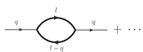
Figure 2: The first term in the so-called skeleton expansion of the two-point function. Heavy lines denote full propagators.

Clearly the spectral forms and their inter-relations derived above hold also for the two-point function appearing in eq. (1.1) for the shear viscosity. We begin with four-dimensional Fourier transforms. To calculate the $11$-element of the the retarded two-point function

$$\Pi_{11}^{R}(q)=i\int d^{4}xe^{iq(x-x^{\prime})}\theta(t-t^{\prime})\langle[\pi_{\alpha\beta}(\boldsymbol{x},t),\pi^{\alpha\beta}(\boldsymbol{x}^{\prime},t^{\prime})]\rangle\,,$$ (3.1)

we consider the corresponding time-ordered one,

$$\Pi_{11}(q)=i\int d^{4}xe^{iq(x-x^{\prime})}\langle T\pi_{\alpha\beta}(\boldsymbol{x},t),\pi^{\alpha\beta}(\boldsymbol{x}^{\prime},t^{\prime})\rangle\,,$$ (3.2)

which can be calculated perturbatively. To leading order, it is given by Wick contractions of pion fields in $\pi_{\alpha\beta}$ given by eq. (1.3). In the so-called skeleton expansion, these contractions are expressed in terms of complete propagators (see Fig. 2) to get,

$$\Pi_{11}(q)=i\int\frac{d^{4}l}{(2\pi)^{4}}N(l,q)D_{11}(l)D_{11}(l-q)\,,$$ (3.3)

where $N(l,q)$ is determined by the derivatives acting on the pion fields,

$$N(l,q)=-6\,[\boldsymbol{l}^{2}(\boldsymbol{l}-\boldsymbol{q})^{2}+\frac{1}{3}\{\boldsymbol{l}\cdot(\boldsymbol{l}-\boldsymbol{q})\}^{2}].$$ (3.4)

To work out the $l_{0}$ integral in eq. (3.3), it is more convenient to use $\Lambda_{11}$ given by eq. (2.18) than by eq. (2.19). Closing the contour in the upper or lower half $l_{0}$-plane we get

$$\Pi_{11}(q)=\int\frac{d^{3}l}{(2\pi)^{3}}N(\boldsymbol{l},\boldsymbol{q})\int\frac{dk_{0}^{\prime}}{2\pi}\rho(k_{0}^{\prime},\boldsymbol{l})\frac{dk_{0}^{\prime\prime}}{2\pi}\rho(k_{0}^{\prime\prime},\boldsymbol{l}-\boldsymbol{q})K(q_{0},k_{0}^{\prime},k_{0}^{\prime\prime})\,,$$ (3.5)

where

$$K=\frac{\{1+f(k_{0}^{\prime})\}f(k_{0}^{\prime\prime})}{q_{0}-(k_{0}^{\prime}-k_{0}^{\prime\prime})+i\eta}-\frac{f(k_{0}^{\prime})\{1+f(k_{0}^{\prime\prime})\}}{q_{0}-(k_{0}^{\prime}-k_{0}^{\prime\prime})-i\eta}\,.$$ (3.6)

The imaginary part of $\Pi_{11}$ arises from the factor $K$,

$${\rm Im}K = -\pi\left[\{1+f(k_{0}^{\prime})\}f(k_{0}^{\prime\prime})+f(k_{0}^{\prime})\{1+f(k_{0}^{\prime\prime})\}\right]\delta(q_{0}-(k_{0}^{\prime}-k_{0}^{\prime\prime}))$$ (3.7)

$$= -\pi\coth(\beta q_{0}/2)\{f(k_{0}^{\prime\prime})-f(k_{0}^{\prime})\}\delta(q_{0}-(k_{0}^{\prime}-k_{0}^{\prime\prime}))\,,$$

while its real part is given by the principal value integrals.

Having obtained the real and imaginary parts of $\Pi_{11}(q)$, we use relations similar to eq. (2.22) to build the $11$-element of the diagonalised $\Pi$ matrix,

$$\overline{\Pi}=\int\frac{d^{3}l}{(2\pi)^{3}}N(\boldsymbol{l},\boldsymbol{q})\int\frac{dk_{0}^{\prime}}{2\pi}\rho(k_{0}^{\prime},\boldsymbol{l})\int\frac{dk_{0}^{\prime\prime}}{2\pi}\rho(k_{0}^{\prime\prime},\boldsymbol{l}-\boldsymbol{q})\frac{\{1+f(k_{0}^{\prime})\}f(k_{0}^{\prime\prime})-f(k_{0}^{\prime})\{1+f(k_{0}^{\prime\prime})\}}{q_{0}-(k_{0}^{\prime}-k_{0}^{\prime\prime})+i\eta\epsilon(q_{0})}\,.$$ (3.8)

Finally $\overline{\Pi}$ can be continued to $\Pi_{11}^{R}$ by a relation similar to eq. (2.30),

$$\Pi^{R}_{11}=\int\frac{d^{3}l}{(2\pi)^{3}}N(\boldsymbol{l},\boldsymbol{q})\int\frac{dk_{0}^{\prime}}{2\pi}\rho(k_{0}^{\prime},\boldsymbol{l})\frac{dk_{0}^{\prime\prime}}{2\pi}\rho(k_{0}^{\prime\prime},\boldsymbol{l}-\boldsymbol{q})\frac{\{1+f(k_{0}^{\prime})\}f(k_{0}^{\prime\prime})-f(k_{0}^{\prime})\{1+f(k_{0}^{\prime\prime})\}}{q_{0}-(k_{0}^{\prime}-k_{0}^{\prime\prime})+i\eta}\,.$$ (3.9)

Note that in eqs. (3.8,3.9) we retain the $f(k_{0}^{\prime})f(k_{0}^{\prime\prime})$ terms in the numerator to put it in a more convenient form. Change the signs of $k_{0}^{\prime}$ and $k_{0}^{\prime\prime}$ in the first and second term respectively. Noting relations like $1+f(-k_{0})=-f(k_{0})$ and $\rho(-k_{0})=-\rho(k_{0})$ we get

$$\Pi^{R}_{11}(q)=\int\frac{d^{3}l}{(2\pi)^{3}}N(\boldsymbol{l},\boldsymbol{q})\int\frac{dk_{0}^{\prime}}{2\pi}\frac{dk_{0}^{\prime\prime}}{2\pi}\rho(k_{0}^{\prime},\boldsymbol{l})\rho(k_{0}^{\prime\prime},\boldsymbol{l}-\boldsymbol{q})f(k_{0}^{\prime})f(k_{0}^{\prime\prime})W(q_{0},k_{0}^{\prime}+k_{0}^{\prime\prime})\,,$$ (3.10)

where

$$W=\frac{1}{q_{0}+k_{0}^{\prime}+k_{0}^{\prime\prime}+i\eta}-\frac{1}{q_{0}-(k_{0}^{\prime}+k_{0}^{\prime\prime})+i\eta}\,.$$ (3.11)

Returning to the expression (1.1) for $\eta$, we now get the three-dimensional spatial integral of the retarded correlation function by setting $\boldsymbol{q}=0$ in eq. (3.1) and Fourier inverting with respect to $q_{0}$,

$$i\int d^{3}x^{\prime}\,\theta(-t^{\prime})\langle[\pi^{\alpha\beta}(\vec{0},0),\pi_{\alpha\beta}(\boldsymbol{x}^{\prime},t^{\prime})]\rangle=-\int dq_{0}\,e^{iq_{0}t^{\prime}}\Pi^{R}_{11}(q_{0},\boldsymbol{q}=0)\,.$$ (3.12)

This completes our use of the real time formulation to get the required result. The integrals appearing in the expression for $\eta$ have been evaluated in Refs. Hosoya ; Lang , which we describe below for completeness.

As shown in Ref. Hosoya , the integral over $t_{1},\,t^{\prime}$ and $q_{0}$ in eqs. (1.1) and (3.12) may be carried out trivially to give

$$\eta=\left.\frac{i}{10}\frac{d}{dq_{0}}\Pi^{R}_{11}(q_{0})\right|_{q_{0}=0}\,.$$ (3.13)

The $q_{0}$ dependence of $\Pi^{R}_{11}$ is contained entirely in $W$,

$$\left.\frac{d}{dq_{0}}W(q_{0})\right|_{q_{0}=0}=-\frac{1}{(k_{0}^{\prime}+k_{0}^{\prime\prime}-i\eta)^{2}}+\frac{1}{(k_{0}^{\prime}+k_{0}^{\prime\prime}+i\eta)^{2}}=2\pi i\delta^{\prime}(k_{0}^{\prime}+k_{0}^{\prime\prime})\,.$$ (3.14)

Changing the integration variables in eq. (3.10) from $k_{0}^{\prime}$, $k_{0}^{\prime\prime}$ to $\overline{k}_{0}=k_{0}^{\prime}+k_{0}^{\prime\prime}$ and $k_{0}=\frac{1}{2}(k_{0}^{\prime}-k_{0}^{\prime\prime})$ we get

$$\eta=\int\frac{d^{3}l}{(2\pi)^{3}}N(\boldsymbol{l})\int\frac{dk_{0}}{(2\pi)^{2}}F(k_{0},\boldsymbol{l})\,,$$ (3.15)

where

$$F(k_{0},\boldsymbol{l})=\left.\frac{d}{d\overline{k}_{0}}\left\{\rho\!\left(\frac{\overline{k}_{0}}{2}+k_{0},\boldsymbol{l}\right)\rho\!\left(\frac{\overline{k}_{0}}{2}-k_{0},\boldsymbol{l}\right)f\!\left(\frac{\overline{k}_{0}}{2}+k_{0}\right)f\!\left(\frac{\overline{k}_{0}}{2}-k_{0}\right)\right\}\right|_{\overline{k}_{0}=0}\,.$$ (3.16)

It turns out that the integral over $k_{0}$ becomes undefined, if we try to evaluate $F(k_{0})$ with the free spectral function $\rho_{0}(k)$ given by eq. (2.24). As pointed out in Ref. Hosoya , we have to take the spectral function for the complete propagator that includes the self-energy of the pion, leading to its finite width $\Gamma$ in the medium,

$$\rho(k_{0},\boldsymbol{l})=\frac{1}{i}\left[\frac{1}{(k_{0}-i\Gamma)^{2}-\omega^{2}}-\frac{1}{(k_{0}+i\Gamma)^{2}-\omega^{2}}\right]\,,~{}~{}~{}~{}~{}~{}~{}~{}~{}~{}\omega=\sqrt{\boldsymbol{l}^{2}+m^{2}}\,.$$ (3.17)

Then $F(k_{0},\boldsymbol{l})$ becomes

$$F=-8\frac{k_{0}^{2}e^{\beta k_{0}}}{(e^{\beta k_{0}}-1)^{2}}\frac{\beta\Gamma^{2}}{\{(k_{0}-i\Gamma)^{2}-\omega^{2}\}^{2}\{(k_{0}+i\Gamma)^{2}-\omega^{2}\}^{2}}\,,$$ (3.18)

having double poles at $k_{0}=2\pi in/\beta$ for $n=\pm 1,\pm 2,\cdots$ and also at $k_{0}=\pm\omega\pm i\Gamma$. The integral over $k_{0}$ may now be evaluated by closing the contour in the upper/lower half-plane to get

$$\int^{+\infty}_{-\infty}\frac{dk_{0}}{(2\pi)^{2}}F(k_{0},\boldsymbol{l})=-\frac{1}{8\pi}\frac{\beta}{\omega^{2}\Gamma}n(\omega)\{1+n(\omega)\}\,,$$ (3.19)

where we retain only the leading (singular) term for small $\Gamma$. In this approximation eq. (3.15) gives Lang

$$\eta=\frac{\beta}{10\pi^{2}}\int_{0}^{\infty}dl\,l^{6}\frac{n(\omega)\{1+n(\omega)\}}{\omega^{2}\Gamma}\,.$$ (3.20)

The width $\Gamma(l)$ at different temperatures is known Goity from chiral perturbation theory Gasser , using which $\eta$ has been evaluated numerically  Lang .

IV Conclusion

Here we calculate a transport coefficient in the real time version of thermal field theory. It is simpler to the imaginary version in that we do not have to continue to imaginary time at any stage of the calculation. As an element in the theory of linear response, a transport coefficient is defined in terms of a retarded thermal two-point function of the components of the energy-momentum tensor. We derive Källen-Lehmann representation for any (bosonic) two-point function of both time-ordered and retarded types to get the relation between them. Once this relation is obtained, we can calculate the retarded function in the Feynman-Dyson framework of the perturbation theory.

Clearly the method is not restricted to transport coefficients. Any linear response leads to a retarded two-point function, which can be calculated in this way. Also quadratic response formulae have been derived in the real time formulation Carrington .

References

(1)
(2) T. Matsubara, Prog. Theor. Phys. 14, 351 (1955)
(3) R. Mills, Propagators for Many Particle Systems, Gordon and
Breach, New York, 1969
(4) H. Matsumoto, Y. Nakano and H. Umezawa, J. Math. Phys. 25,
3076 (1984)
(5) A.J. Niemi and G.W. Semenoff, Ann. Phys. 152, 105 (1984).