Density fluctuations and the acceleration of electrons by beam-generated Langmuir waves in the solar corona

Abstract

Non-thermal electron populations are observed throughout the heliosphere. The relaxation of an electron beam is known to produce Langmuir waves which, in turn, may substantially modify the electron distribution function. As the Langmuir waves are refracted by background density gradients and as the solar and heliospheric plasma density is naturally perturbed with various levels of inhomogeneity, the interaction of Langmuir waves with non-thermal electrons in inhomogeneous plasmas is an important topic. We investigate the role played by ambient density fluctuations on the beam-plasma relaxation, focusing on the effect of acceleration of beam electrons. The scattering of Langmuir waves off turbulent density fluctuations is modeled as a wavenumber diffusion process which is implemented in numerical simulations of the one-dimensional quasilinear kinetic equations describing the beam relaxation. The results show that a substantial number of beam electrons are accelerated when the diffusive time scale in wavenumber space $\tau_{D}$ is of the order of the quasilinear time scale $\tau_{ql}$, while when $\tau_{D}\ll\tau_{ql}$, the beam relaxation is suppressed. Plasma inhomogeneities are therefore an important means of energy redistribution for waves and hence electrons, and so must be taken into account when interpreting, for example, hard X-ray or Type III emission from flare-accelerated electrons.

1. Introduction

The relaxation of an electron beam producing Langmuir waves is a fundamental process in space and laboratory plasmas. As the Langmuir waves interact with the fast electrons, and their dynamics are strongly affected by variations in the ambient plasma density and as the heliospheric plasma density is perturbed with different levels of inhomogeneity, the interaction of Langmuir waves with non-thermal electrons in turbulent inhomogeneous plasmas is an important topic in astrophysics.

In the solar atmosphere, the beam-plasma instability is known to be the cause of Type III radio bursts, with their characteristic rapid frequency drift being a result of the beam propagation through the decreasing density coronal plasma (Ginzburg & Zhelezniakov 1958; Zheleznyakov & Zaitsev 1970; Melrose 1990). Numerical simulations of the beam relaxation in the inhomogeneous plasma of the solar wind can reproduce the broken power-law in the electron flux spectrum which is observed near the Earth for impulsive solar electron events (Reid & Kontar 2010). In solar flare environments, it has been shown that the beam relaxation is likely to cause spectral index variations inferred from hard X-ray observations (e.g. Hannah et al. 2009).

It was recognized already in the context of beam-plasma experiments (Breǐzman & Ryutov 1969; Liperovskii & Tsytovich 1965) that the mere existence of an inhomogeneity in the ambient plasma density was sufficient to produce a redistribution of Langmuir wave energy in wavenumber space. This idea was proposed in order to explain the common observations of electrons with energy above the injected one (Breǐzman & Ryutov 1969) in laboratory experiments such as those carried out by Berezin et al. (1964) on powerful relativistic beams. The interaction between the waves and the beam electrons is resonant, which implies that the spectral transfer of wave energy toward lower/higher wavenumbers allows interaction with faster/slower electrons respectively. Various mechanisms may cause this spectral energy transfer, they may involve regular or random density variations, or non-linear interactions between Langmuir waves and low-frequency electrostatic compressive modes. For example, it is known that ion-sound waves can effectively scatter Langmuir waves to smaller wavenumbers (e.g., Liperovskii & Tsytovich 1965; Melrose 1974; Escande 1975; Papadopoulos 1975; Escande & de Genouillac 1978). Low-frequency electromagnetic modes, such as kinetic Alfven waves (Bian & Kontar 2010; Bian et al. 2010) are compressive and thus their refractive power may also have a substantial effect on the spectral evolution of beam-driven Langmuir waves. Numerical simulations of the beam relaxation in a plasma with a constant density gradient were conducted in (e.g. Krasovskii 1978; Kontar 2001; Tsiklauri 2010) and the combination of a regular density gradient with allowance for the non-linear coupling to ion sound waves was considered by Kontar & Pécseli (2002); Yoon et al. (2006); Ziebell et al. (2011), with the result that a very high level of Langmuir waves was produced at small wavenumbers. The simulations by Kontar et al. (2012) found that a fluctuating density could lead to the appearance of accelerated electrons in a collisionally-relaxing electron beam.

Vedenov et al. (1967) first described the effect of random large scale density inhomogeneities as a diffusive transfer of Langmuir wave energy in wavenumber space. This diffusion equation was used by Nishikawa & Ryutov (1976) to describe the process of elastic scattering off random and time-independent density fluctuations, (see also Goldman & Dubois 1982; Muschietti & Dum 1991). Elastic scattering results only in angular diffusion in wave-number space, and for the case of waves generated by beam electrons with a small angular spread, wave energy is transferred away from the region of excitation in $k$-space, which may lead to suppression of the beam-plasma instability. Neglecting the effect of wave reabsorption on the electrons, the role of the angular diffusion term has been accounted for in the kinetic equations describing the beam-plasma system, by replacing it by a wave damping term (Muschietti et al. 1985; Melrose 1987). However, in general, energy conservation dictates that reabsorption of wave energy by the beam is accompanied by an acceleration of the electrons. In addition, inelastic scattering results in a change in the absolute value of the Langmuir wavenumber, which may produce acceleration in the projected electron distribution.

Here, we consider anew this important topic of beam relaxation in a fluctuating plasma. In Section II, we derive a general expression for the diffusion coefficient in wavenumber space. In Section III, the wavenumber diffusion is implemented in numerical simulations of the one-dimensional kinetic equations describing the quasilinear evolution of the beam-plasma instability. We focus on the effect of acceleration of beam electrons in a fluctuating plasma and derive a condition for it to occur. In Section IV, we generalize the discussion to 3D and discuss the role of both elastic and inelastic scattering in the acceleration of fast electrons. A summary of the results is presented in Section V.

2. Langmuir wave scattering and diffusion: 1D case

Let us start by considering a one-dimensional problem where the dynamics of both electrons and Langmuir waves are along $x$, the direction of the external magnetic field. The plasma density is written as $n_{e}[1+\tilde{n}(x,t)]$ with $n_{e}$ the constant background density and $\tilde{n}(x,t)$ the relative density fluctuation, which is assumed to be weak, i.e. $\tilde{n}(x,t)\ll 1$, a condition often satisfied in the solar corona and the solar wind.

In general, the characteristic wavenumber $q$ of low-frequency density fluctuations is much smaller than the characteristic wavenumber $k$ associated with high-frequency Langmuir waves, so we can make the WKB approximation and treat the Langmuir waves as quasi-particles. Ambient density fluctuations are associated with a change in the local refractive index experienced by the waves, and in the low frequency limit the Langmuir wave dynamics can thus be modeled by Hamilton’s equations of motion for the quasi-particles (e.g. Whitham 1965; Vedenov et al. 1967; Zakharov 1974), which are given by

$$\frac{dk}{dt}=-\frac{1}{2}\omega_{pe}\frac{\partial\tilde{n}}{\partial x}\equiv F(x,t)$$ (1)

$$\frac{dx}{dt}={\mathrm{v}}_{g}$$ (2)

where $F(x,t)$ is the ”refraction force” acting on the wave-packets, ${\mathrm{v}}_{g}=3{\mathrm{v}}_{Te}^{2}k/\omega_{pe}$ is the group velocity and $\omega_{pe}$ is the local plasma frequency $\omega_{pe}=\sqrt{4\pi n_{e}e^{2}/m_{e}}$.

Equivalently, we can write a conservation relation describing the evolution of the spectral energy density associated with Langmuir waves $W(x,k,t)$ [erg cm^-2]

$$\frac{\partial W(x,k,t)}{\partial t}+{\mathrm{v}}_{g}\frac{\partial W(x,k,t)}{\partial x}-F(x,t)\frac{\partial W(x,k,t)}{\partial k}=0,$$ (3)

where $W(x,k,t)$ is normalised to the energy density of Langmuir waves $E=\int W(x,k,t)dk$.

From Equation (1) we see that random refraction induces stochastic change in the wavenumber, resulting in diffusion of the spectral energy density in $k$-space. An expression for the diffusion coefficient $D$ is derived from the phase-space conservation equation (3) following standard procedures (e.g. Vedenov & Velikhov 1963; Sturrock 1966), as follows.

The spectral energy density of Langmuir waves $W(x,k,t)$ is decomposed into the sum of its average and fluctuating parts as $W=\langle W\rangle+\widetilde{W}$. Substituting this expression into Eq. (3) gives one equation for the average

$$\frac{\partial\langle W\rangle}{\partial t}=-\langle F(x,t)\frac{\partial\widetilde{W}}{\partial k}\rangle$$ (4)

and one equation for the fluctuations

$$\frac{\partial\widetilde{W}}{\partial t}+{\mathrm{v}}_{g}\frac{\partial\widetilde{W}}{\partial x}=-F(x,t)\frac{\partial\langle W\rangle}{\partial k}$$ (5)

where a term quadratic in the fluctuation amplitude has been neglected since the latter is assumed to be weak. Equation (5) is integrated to give

$$\widetilde{W}(x,k,t)=-\int_{0}^{t}d\tau F(x-{\mathrm{v}}_{g}\tau,t-\tau)\frac{\partial\langle W\rangle(x-{\mathrm{v}}_{g}\tau,k,t-\tau)}{\partial k},$$ (6)

which is substituted into Eq. (4) to give the equation describing the diffusion of wave energy in $k$-space,

$$\frac{\partial\langle W\rangle}{\partial t}=\frac{\partial}{\partial k}D\frac{\partial\langle W\rangle}{\partial k},$$ (7)

where the diffusion coefficient $D$ is expressed in terms of the auto-correlation function of the refraction force as

$$D=\int_{0}^{\infty}d\tau\langle F(x,t)F(x-{\mathrm{v}}_{g}\tau,t-\tau)\rangle.$$ (8)

The Fourier components $F(q,\Omega)$ and the spectrum $S_{F}(q,\Omega)$ of $F(x,t)$ are defined through $F(x,t)=\int_{-\infty}^{\infty}dq\int_{-\infty}^{\infty}d\Omega F(q,\Omega)\exp{[2\pi i(qx-\Omega t)]}dkd\Omega$ and $\langle F(q,\Omega)F(q^{\prime},\Omega^{\prime})\rangle=S_{F}(q,\Omega)\delta(q+q^{\prime})\delta(\Omega+\Omega^{\prime})$, respectively. As a consequence, the diffusion coefficient can be written in terms of $S_{F}(q,\Omega)$ as

$$D=\frac{1}{2}\int_{-\infty}^{\infty}dq\int_{-\infty}^{\infty}d\Omega S_{F}(q,\Omega)\delta(\Omega-q{\mathrm{v}}_{g}).$$ (9)

Since the spectrum of the refraction force $S_{F}(q,\Omega)$ is related to the spectrum of ambient plasma density fluctuations $S_{n}(q,\Omega)$ by $S_{F}(q,\Omega)=\omega_{pe}^{2}(\pi q)^{2}S_{n}(q,\Omega)$, the diffusion coefficient can finally be expressed as

$$D=\frac{\omega_{pe}^{2}\pi^{2}}{2}\int_{-\infty}^{\infty}dq\int_{-\infty}^{\infty}d\Omega\;q^{2}S_{n}(q,\Omega)\delta(\Omega-q{\mathrm{v}}_{g}),$$ (10)

where by definition $\langle\tilde{n}^{2}\rangle=\int_{-\infty}^{\infty}dq\int_{-\infty}^{\infty}d\Omega\;S_{n}(q,\Omega)$.

According to Eq. (10), a quasi-particle with wave-number $k$ interacts with a Fourier mode $(\Omega,q)$ of the density fluctuation spectrum for which the resonance condition $\Omega=q{\mathrm{v}}_{g}$ is satisfied, which also means that $(\Omega/q)(\omega_{pe}/k)=3{\mathrm{v}}_{Te}^{2}$. In the particular case where density fluctuations are due to waves with a dispersion relation $\Omega=\Omega(q)$, then $S_{n}(q,\Omega)=S_{n}(q)\delta(\Omega-\Omega(q))$ and $D=(\omega_{pe}^{2}\pi^{2}/2)\int_{-\infty}^{\infty}dqq^{2}S_{n}(q)\delta(\Omega(q)-q{\mathrm{v}}_{g})$.

For a Gaussian spectrum

$$S_{n}(q,\Omega)=\frac{\langle\tilde{n}^{2}\rangle}{\pi q_{0}\Omega_{0}}\exp\left(-\frac{q^{2}}{q_{0}^{2}}-\frac{\Omega^{2}}{\Omega_{0}^{2}}\right)$$ (11)

where $q_{0}$ and $\Omega_{0}$ are characteristic wavenumber and frequency, the diffusion coefficient reads

$$D=\omega_{pe}^{2}{\pi}^{3/2}\frac{q_{0}}{{\mathrm{v}}_{0}}\langle\tilde{n}^{2}\rangle\left(1+\frac{{\mathrm{v}}_{g}^{2}}{{\mathrm{v}}_{0}^{2}}\right)^{-3/2},$$ (12)

where ${\mathrm{v}}_{0}=\Omega_{0}/q_{0}$.

The diffusion coefficient depends on wave-number $k$ through the group velocity ${\mathrm{v}}_{g}=3{\mathrm{v}}_{Te}^{2}k/\omega_{pe}$. From Eq. (12), we see that for a Gaussian spectrum there are two regimes of wavenumber diffusion. When the decorrelation velocity associated with ambient density fluctuations ${\mathrm{v}}_{0}$ is much larger than the group velocity of the Langmuir waves, i.e. when ${\mathrm{v}}_{0}\gg{\mathrm{v}}_{g}$, then

$$D=\omega_{pe}^{2}{\pi}^{3/2}\left(\frac{q_{0}}{{\mathrm{v}}_{0}}\right)\langle\tilde{n}^{2}\rangle,$$ (13)

an expression which is independent of ${\mathrm{v}}_{g}$ and hence $k$. Conversely, when ${\mathrm{v}}_{0}\ll{\mathrm{v}}_{g}$, then

$$D=\omega_{pe}^{2}{\pi}^{3/2}\left(\frac{q_{0}}{{\mathrm{v}}_{0}}\right)\left(\frac{{\mathrm{v}}_{0}}{{\mathrm{v}}_{g}}\right)^{3}\langle\tilde{n}^{2}\rangle,$$ (14)

and the wavenumber diffusion becomes $k$ dependent.

It is also interesting to consider compressive fluctuations at a given characteristic frequency, so that $S_{n}(q,\Omega)=S_{n}(q)\delta(\Omega-\Omega_{0})$, with a power-law spectrum in wavenumber space with spectral index $\zeta>1$, as observed in the solar wind (e.g. Cronyn 1972; Celnikier et al. 1983; Robinson 1983). Then

$$S_{n}(q,\Omega)=\langle\tilde{n}^{2}\rangle\left(\frac{\zeta-1}{q_{0}}\right)\left(\frac{q}{q_{0}}\right)^{-\zeta}\delta(\Omega-\Omega_{0})$$ (15)

for $q>q_{0}$ and zero elsewhere. In this case we find that

$$D=\frac{\omega_{pe}^{2}\pi^{2}}{2}(\zeta-1)\left(\frac{q_{0}}{{\mathrm{v}}_{0}}\right)\left(\frac{{\mathrm{v}}_{0}}{{\mathrm{v}}_{g}}\right)^{3-\zeta}\langle\tilde{n}^{2}\rangle.$$ (16)

Comparison of this last expression with Eq. (14) shows how the spectrum of density fluctuations affects the wavenumber dependence of the diffusion coefficient $D$.

3. Numerical results

We now perform numerical simulations of the quasilinear kinetic equations describing wave-particle interactions. These equations are based on those given by Vedenov & Velikhov (1963); Vedenov et al. (1967); Tsytovich (1995) adding a spontaneous wave emission term as in Zheleznyakov & Zaitsev (1970); Hannah et al. (2009); Reid et al. (2011) and collisional operators as in e.g Lifshitz & Pitaevskii (1981):

$$\frac{\partial f}{\partial t}=\frac{4\pi^{2}e^{2}}{m_{e}^{2}}\frac{\partial}{\partial{\mathrm{v}}}\left(\frac{W}{{\mathrm{v}}}\frac{\partial f}{\partial{\mathrm{v}}}\right)+\Gamma\frac{\partial}{\partial\mathrm{v}}\left(\frac{f}{\mathrm{v}^{2}}+\frac{\mathrm{v}_{Te}^{2}}{\mathrm{v}^{3}}\frac{\partial f}{\partial\mathrm{v}}\right),\;\;\;$$ (17)

$$\frac{\partial W}{\partial t}=\frac{\omega_{pe}^{3}m_{e}}{4\pi n_{e}}\mathrm{v}\ln\left(\frac{\mathrm{v}}{\mathrm{v}_{Te}}\right)+\frac{\pi\omega_{pe}^{3}}{n_{e}k^{2}}W\frac{\partial f}{\partial{\mathrm{v}}}-\frac{\Gamma}{4{\mathrm{v}}_{Te}^{3}}W+\frac{\partial}{\partial k}\left(D\frac{\partial W}{\partial k}\right),$$ (18)

where $\Gamma=4\pi e^{4}n_{e}\ln\Lambda/m_{e}^{2}$, with $\ln\Lambda\simeq 20$ the Coulomb logarithm. The last term in Eq. (18) describes the effect of wavenumber diffusion produced by the ambient density fluctuations, as discussed in the previous section.

The initial electron distribution function $f({\mathrm{v}},t)$ [electrons cm^-3 (cm/s)^-1 ] is chosen as the superposition of a Maxwellian background and a Maxwellian beam:

$$f({\mathrm{v}},t=0)=\frac{n_{e}}{\sqrt{2\pi}{\mathrm{v}}_{Te}}\exp\left(-\frac{{\mathrm{v}}^{2}}{2{\mathrm{v}}_{Te}^{2}}\right)+\frac{n_{b}}{\sqrt{\pi}\Delta{\mathrm{v}}_{b}}\exp\left(-\frac{({\mathrm{v}}-{\mathrm{v}}_{b})^{2}}{\Delta{\mathrm{v}}_{b}^{2}}\right)$$ (19)

and the initial spectral energy density of Langmuir waves $W(k,t)$ [ergs cm^-2 ] is set to the thermal level:

$$W(k,t=0)=\frac{k_{b}T_{e}}{4\pi^{2}}k^{2}\ln\left(\frac{1}{k\lambda_{de}}\right).$$ (20)

Except where otherwise stated, the simulations below assume a background plasma with $T_{e}=T_{i}=1$MK and $\omega_{pe}/2\pi=1GHz$ giving a background density of $n_{e}=1.2\times 10^{10}$cm^-3. The beam parameters are $n_{b}=10^{5}\simeq 10^{-5}n_{e}$, ${\mathrm{v}}_{b}=5\times 10^{9}$cms^-1 and $\Delta{\mathrm{v}}_{b}=0.3{\mathrm{v}}_{b}$. The spectrum of background density fluctuations is taken first to be Gaussian, so the diffusion coefficient $D$ is given by Eq. (12). We fix $q_{0}=10^{-4}k_{De}$. The magnitude of relative density fluctuations $\sqrt{\langle\tilde{n}^{2}\rangle}$ ranges between $10^{-4}$ and $10^{-1}$, and ${\mathrm{v}}_{0}$ is taken between $0.01{\mathrm{v}}_{Te}$ and ${\mathrm{v}}_{Te}$.

Figure (1) is divided into four distinct panels which all show the evolution of the electron and the wave distributions as the intensity of the background density fluctuations $\sqrt{\langle\tilde{n}^{2}\rangle}$ is increased. In a homogeneous plasma, as shown in the top left panel, the electron beam is unstable to the generation of Langmuir waves, which grow at a rate given by

$$\gamma\sim\frac{n_{b}}{n_{e}}\omega_{pe}.$$ (21)

The spectrum of Langmuir waves interacts with the beam electrons and causes them to diffuse in the resonant region in velocity space, given by $\omega_{pe}=k{\mathrm{v}}$, until the distribution function reaches a plateau, on a time scale given by the quasilinear time:

$$\tau_{ql}=\frac{1}{\omega_{pe}}\frac{n_{e}}{n_{b}}.$$ (22)

By time $t=100\tau_{ql}$, the beam has fully relaxed and the electron distribution is flat between $6{\mathrm{v}}_{Te}$ ($E=1.5$ keV) and $16{\mathrm{v}}_{Te}$ ($11$ keV), as shown by the red lines in Figure 1. The collisional timescale, $\tau_{coll}={\mathrm{v}}_{Te}^{3}/\Gamma$ and the timescale for collisional destruction of the plateau, $\tau_{coll}({\mathrm{v}/{\mathrm{v}}_{Te}})^{3}\sim 1$ s at ${\mathrm{v}}=15{\mathrm{v}}_{Te}$ are both far longer than the quasilinear time. Collisional effects are therefore negligible. This remains true for the various values of beam density and background plasma parameters which will be considered below.

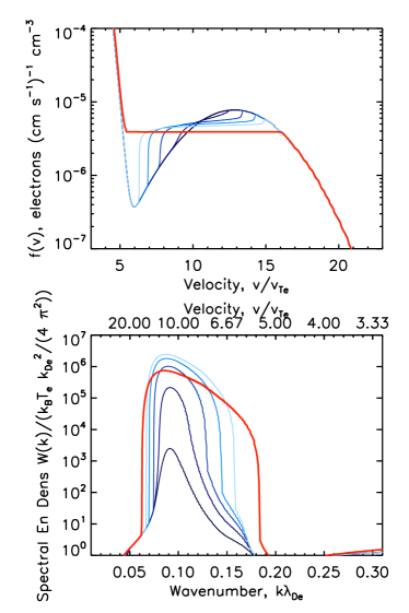
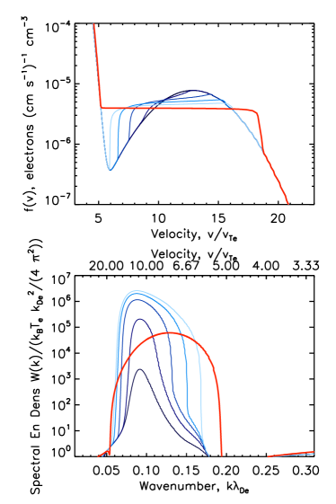
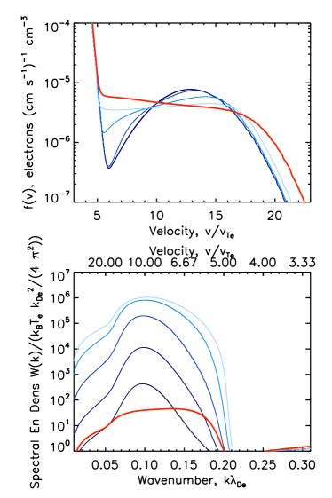
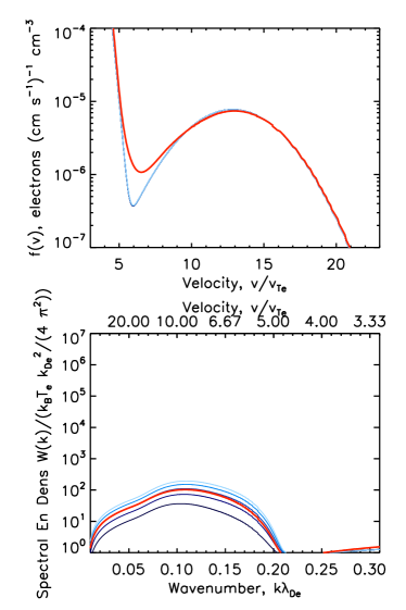
Figure 1.— Electron distribution $f(\mathrm{v})$ (upper plots), and Langmuir wave spectral energy density $W(k)$ (lower plots) for homogeneous (top left) and inhomogeneous plasma, with $q_{0}=10^{-4}k_{de}$, ${\mathrm{v}}_{0}/{\mathrm{v}}_{Te}=0.3$ and $\sqrt{\langle\tilde{n}^{2}\rangle}$ of $3.7\times 10^{-4}$ (top right), $3.7\times 10^{-3}$ (bottom left) and $1.2\times 10^{-2}$ (bottom right). Lines from dark (blue in online version) to light show the beam relaxation during the first ten quasilinear times, while the thick line (red in online version) shows the state reached at $t=100\tau_{ql}$.

A finite level of background density fluctuations produces diffusion of the waves in $k$-space which allows them to interact resonantly with electrons from a larger region of velocity space. In other words, the region of resonant wave-particle interaction is broadened due to the random wave refraction induced by the ambient density perturbations. This effect is well illustrated by the bottom left panel of Figure 1 which shows the electron and wave distributions for a moderate level of density fluctuations, $\sqrt{\langle\tilde{n}^{2}\rangle}=3.7\times 10^{-3}$. The Langmuir wave spectrum diffuses in wavenumber, widening the beam distribution and slowing the plateau formation. The electron distribution $f({\mathrm{v}})$ is increased from the upper edge of the plateau to the highest velocities in the simulation, implying that electrons have been accelerated. In addition, the increased level of waves at large wavenumbers has a visible effect on the electron distribution down to around $6{\mathrm{v}}_{Te}$.

The top right panel shows very weak density fluctuations, with $\sqrt{\langle\tilde{n}^{2}\rangle}=3.7\times 10^{-4}$. The beam relaxes in a manner similar to the homogeneous case but the wave spectrum is broadened slightly in $k$-space, resulting in a wider plateau in the electron distribution.

When the inhomogeneity becomes very strong, as illustrated by the bottom right panel where $\sqrt{\langle\tilde{n}^{2}\rangle}=1.2\times 10^{-2}$, diffusion still transports the waves out of their region of excitation in $k$-space but on a timescale which is much smaller than their growth rate, so the wave level is barely increased above the thermal level. As we can see, by time $t=100\tau_{ql}$ the electron distribution remains essentially unchanged from the initial distribution. The main point is that for intense density fluctuations, diffusive broadening of the Langmuir wave spectrum becomes large enough for the waves to be mainly reabsorbed by the thermal electrons at $k\lambda_{De}\sim 1$. Since the energy density of waves generated is much smaller than the thermal energy of plasma, the effect on the distribution function of thermal particles is negligible. This is the suppression regime of the beam-plasma instability which has often been discussed in the past, mainly in the context of the role of angular diffusion of wave energy induced by elastic scattering in 3D. As shown here, the suppression of the beam-plasma instability can also occur as a result of inelastic scattering. Here, we focus on the effect of electron acceleration due to wave reabsorption by the beam electrons as opposed to reabsorption by the the thermal electrons. A discussion of electron acceleration in 3D, as a result of both elastic and inelastic scattering, is presented in the next section.

Clearly, the main effect of increasing the level of density fluctuations is to increase the rate at which wave energy is transported in $k$-space. The time scale associated with such diffusive process is

$$\tau_{D}=\frac{(\Delta k_{b})^{2}}{D(k_{b})}$$ (23)

where $k_{b}=\omega_{pe}/{\mathrm{v}}_{b}$ and $\Delta k_{b}=\omega_{pe}(\Delta{\mathrm{v}}_{b}/{\mathrm{v}}_{b}^{2})$ , with parameters $\omega_{pe},{\mathrm{v}}_{b}$ and $\Delta{\mathrm{v}}_{b}$ as given above. Therefore, it is natural to define a non-dimensional number $R$, which is the ratio of the diffusion time $\tau_{D}$ and the quasilinear time $\tau_{ql}$, i.e.

$$R=\frac{\tau_{D}}{\tau_{ql}}.$$ (24)

Figure 2.— The total energy of beam (left) and tail (middle) electrons, both normalised to the initial beam energy $E_{0}$, and the average energy of a tail electron (right), all evaluated at $t=100\tau_{ql}$, against the parameter $R=\tau_{D}/\tau_{ql}$, which gives a measure of the degree of inhomogeneity. Beam and plasma parameters, and ranges for $\sqrt{\langle\tilde{n}^{2}\rangle}$ and ${\mathrm{v}}_{0}$ are as given in the text. The asterisks mark the three levels of inhomogeneity shown in Figure 1. The dashed lines are polynomial fits to the data to illustrate its general trends.

To quantify things further, let us define a “beam” region in velocity space that includes all electrons with velocity above $6{\mathrm{v}}_{Te}$, and a “tail” region above $16{\mathrm{v}}_{Te}$. The energy of the initial Maxwellian beam is given by $E_{0}$. We can then determine the total energy in the beam and tail electrons at time $t=100\tau_{ql}$, which indicates the extent to which the beam relaxation is suppressed and electrons are accelerated. In the homogeneous case, $E_{beam}=0.76E_{0}$ and $E_{tail}=0.2E_{0}$ respectively. In Figure 2, we plot the ratios $E_{beam}/E_{0}$, $E_{tail}/E_{0}$ and $E_{tail}/n_{tail}$ at $t=100\tau_{ql}$ as functions of the parameter $R$, for a range of values of $\sqrt{\langle\tilde{n}^{2}\rangle}$ and ${\mathrm{v}}_{0}$. The three cases in Figure 1 are marked by asterisks, and represent three distinct regions in $R$. In the strong inhomogeneity case, with $\sqrt{\langle\tilde{n}^{2}\rangle}=1.2\times 10^{-3}$ and $R\ll 1$, the beam-plasma instability is suppressed, so the beam remains close to its initial Maxwellian form and we find $E_{beam}=0.99E_{0}$ and $E_{tail}=0.21E_{0}$. Very weak inhomogeneity, with $\sqrt{\langle\tilde{n}^{2}\rangle}=3.7\times 10^{-4}$ corresponding to $R\gg 1$, has little effect on the beam relaxation, so the beam energy is close to the homogeneous value, but the tail energy is slightly increased due to the broadened plateau, giving $E_{beam}=0.78E_{0}$ and $E_{tail}=0.23E_{0}$ The intermediate case, with $\sqrt{\langle\tilde{n}^{2}\rangle}=3.7\times 10^{-3}$ and $R\sim 1$, gives $E_{beam}=0.95E_{0}$ and $E_{tail}=0.35E_{0}$. Both the total tail electron energy (middle panel) and the average energy of a tail electron (right panel), show a significant increase over more than two orders of magnitude in $R$ around $R\sim 1$. To summarize we have identified three distinct regimes of the beam plasma instability in a fluctuating plasma which are controlled by the parameter $R$. When $R\gg 1$, the density fluctuations have a weak refractive power and the relaxation proceeds as in a homogeneous plasma. When $R\ll 1$, diffusive broadening of the wave spectrum is large, the waves are mainly reabsorbed by the thermal particles, their level stays small and the instability is suppressed. When $R\sim 1$ diffusive broadening of the wave spectrum is such that a substantial part of the wave energy is now also reabsorbed by the beam electrons leading to acceleration of the beam particles. Using Eq. (12), we may express the condition for strong acceleration, $R\sim 1$ as

$$\frac{n_{b}}{n_{e}}\left(\frac{\Delta{\mathrm{v}}_{b}}{{\mathrm{v}}_{b}}\right)^{2}\sim\langle\tilde{n}^{2}\rangle\frac{q_{0}^{2}{\mathrm{v}}_{b}^{2}}{{\Omega}_{0}\omega_{pe}}\left(1+\frac{v_{g}^{2}}{v_{0}^{2}}\right)^{-3/2}.$$ (25)

As discussed in Section 2, for a Gaussian spectrum of density fluctuations there are two extreme regimes of wavenumber diffusion, where the characteristic group velocity of the beam driven Langmuir waves, ${\mathrm{v}}_{g}$ is much larger or smaller than ${\mathrm{v}}_{0}$. Let us notice that all of the values for ${\mathrm{v}}_{0}$ used in the above simulations lie in the transitional region ${\mathrm{v}}_{g}\sim{\mathrm{v}}_{0}$. The effect of ${\mathrm{v}}_{0}$ on the $k$-dependence of the diffusion coefficient and hence on $\tau_{D}$ is therefore also important, and accounts for the vertical scatter in the points in Figure 2.

Figure 3.— As Fig.2, the total energy of beam (left) and tail (middle) electrons, both normalised to the initial beam energy $E_{0}$, and the average energy of a tail electron (right), all at $t=100\tau_{ql}$ against $R=\tau_{D}/\tau_{ql}$. Simulation results for various values of the beam, plasma and density fluctuation parameters are shown. Ranges for $\sqrt{\langle\tilde{n}\rangle},{\mathrm{v}}_{0}$ are as in the text. For $\omega_{pe}=1$GHz we show: Gaussian fluctuations with $n_{b}=10^{5}$ (crosses) and $n_{b}=10^{4}$ (squares), powerlaw fluctuations with indices $\frac{5}{3}$ and $\frac{7}{3}$ (triangles). Finally for $\omega_{pe}=200$MHz we show Gaussian fluctuations with $n_{b}=10^{3}$ (diamonds).

Figure 3 shows the total beam and tail energies and average tail electron energy for several values of background density and beam density, for both Gaussian and power-law density fluctuation spectra. The distribution of the beam and tail total energies with respect to the parameter $R$ is essentially unchanged from Figure 2. We note that collisional effects remain unimportant for all parameters chosen. Lower beam densities than those shown produce insufficient levels of Langmuir waves to cause acceleration, and the parameter $R$ is unaffected by changes in local plasma frequency. The results for power-law fluctuation spectra are similar to those for a Gaussian spectrum. We may therefore expect significant electron acceleration to occur whenever $R\sim 1$, regardless of the specific spectrum of fluctuations, or the specific values of the other parameters.

4. Generalization to 3D

Using the same methodology developed for the one-dimensional case, we now generalize the diffusive description of Langmuir waves to three-dimensions. The main difference with the 1D case is that in 3D refraction can change both the absolute value and the orientation of the wavevector $\vec{k}$. The conservation equation for the spectral energy density $W(\vec{x},\vec{k},t)$ [erg], is now

$$\frac{\partial W(\vec{x},\vec{k},t)}{\partial t}+\vec{{\mathrm{v}}}_{g}.\nabla W(\vec{x},\vec{k},t)-\frac{1}{2}\omega_{pe}\nabla\tilde{n}(\vec{x},t)\cdot\frac{\partial W(\vec{x},\vec{k},t)}{\partial\vec{k}}=0,$$ (26)

where $\vec{{\mathrm{v}}_{g}}=(3{\mathrm{v}}_{Te}^{2}/\omega_{pe})\vec{k}$ is the group velocity. In 3D the diffusion equation takes the form

$$\frac{\partial W(\vec{k},t)}{\partial t}=\frac{\partial}{\partial k_{i}}D_{ij}\frac{\partial W(\vec{k},t)}{\partial{k_{j}}}$$ (27)

with the diffusion tensor given by

$$D_{ij}(\vec{k})=2\pi\omega_{pe}^{2}\int d\Omega\int\frac{d^{3}q}{(2\pi)^{3}}\;q_{i}q_{j}S_{n}(\vec{q},\Omega)\delta\left(\Omega-\vec{q}\cdot\vec{{\mathrm{v}}_{g}}\right),$$ (28)

where $S_{n}(\vec{q},\Omega)$ is the spectrum of the density fluctuations and $\int d\mathbf{k}W(\mathbf{k},t)=E$. In the particular case where density fluctuations are due to waves with a dispersion relation $\Omega=\Omega(q)$, then $S_{n}(\vec{q},\Omega)=S_{n}(\vec{q})\delta(\Omega-\Omega(\vec{q}))$ and

$$D_{ij}(\vec{k})=2\pi\omega_{pe}^{2}\int d^{3}q\;q_{i}q_{j}S_{n}(\vec{q})\delta\left(\Omega(\vec{q})-\vec{q}\cdot\vec{{\mathrm{v}}_{g}}\right).$$ (29)

In spherical coordinates with $\vec{k}=(k,\theta,\phi)$, the general equation for diffusion (assuming azimuthal symmetry) is

$$\frac{\partial W(\vec{k},t)}{\partial t}=\left(\frac{1}{k^{2}}\frac{\partial}{\partial k}\left(k^{2}D_{kk}\frac{\partial}{\partial k}\right)+\frac{1}{\sin\theta}\frac{\partial}{\partial\theta}\sin\theta\left(\frac{D_{\theta\theta}}{k^{2}}\frac{\partial}{\partial\theta}\right)\right)W(\vec{k},t)$$ (30)

with coefficients given in the Appendix below by Equation A8.

Expressions for the only non-zero components of the diffusion tensor $D_{kk}$ and $D_{\theta\theta}$ are also derived in the Appendix A and are given by

$$D_{kk}=\frac{\omega_{pe}^{2}}{216\pi{\mathrm{v}}_{Te}^{3}(k\lambda_{de})^{3}}\int dq\Omega(q)^{2}qS_{n}(q)$$ (31)

$$D_{\theta\theta}=\frac{\omega_{pe}^{2}}{24\pi{\mathrm{v}}_{Te}k\lambda_{de}}\int dqq^{3}\left(1-\left(\frac{\Omega(q)}{3{\mathrm{v}}_{Te}k\lambda_{de}q}\right)^{2}\right)S_{n}(q)$$ (32)

Note here that due to the resonance condition $\Omega(q)\leq 3{\mathrm{v}}_{Te}k\lambda_{de}q$ the second expression is always positive.

The particular case of elastic scattering is recovered by setting $\Omega=0$ in Equations (31) and (32) in which case we find that

$$D_{kk}=0$$ (33)

and

$$D_{\theta\theta}=\frac{\omega_{pe}^{2}}{24\pi{\mathrm{v}}_{Te}k\lambda_{de}}\int dqq^{3}S_{n}(q),$$ (34)

as given by Muschietti et al. (1985). Diffusion then occurs in angle only at a rate independent of $\theta$ and tends to isotropise the Langmuir wave spectrum.

It is instructive to rewrite the diffusion equation in terms of the independent variables $k$ and $k_{\parallel}$, where $k_{\parallel}$ is the component of the wavevector parallel to the beam direction, given by $k_{\parallel}=k\cos\theta$. In the limit $\cos\theta\sim 1$, or equivalently $k\sim k_{\parallel}$, we obtain

$$\frac{\partial}{\partial t}W(k_{\parallel},t)=\frac{1}{k_{\parallel}^{2}}\frac{\partial}{\partial k_{\parallel}}\left(k_{\parallel}^{2}D_{kk}\frac{\partial}{\partial k_{\parallel}}\right)W(k_{\parallel},t)-2\frac{D_{\theta\theta}}{k_{\parallel}}\frac{\partial}{\partial k_{\parallel}}W(k_{\parallel},t).$$ (35)

This shows that both magnitude and angular change in wave-vector, as given by $D_{kk}$ and $D_{\theta\theta}$, contribute to the redistribution of wave energy in wavenumber parallel to the beam. This transport of wave energy is diffusive for the former and convective for the latter. In both cases, waves shifted to smaller parallel wavenumbers can be absorbed by beam electrons at larger parallel velocities resulting in acceleration of tail electrons. A large body of work has been devoted to the role of angular diffusion (e.g. Nishikawa & Ryutov 1976) with respect to the suppression of the beam-plasma instability, mainly in the context of elastic scattering, i.e. $D_{kk}=0$. The electron distribution was assumed to be fixed and the effect of scattering of waves by density fluctuations was modeled solely as wave damping. However, the energy lost by the waves due to damping is transferred to the electrons leading to electron acceleration.

A full numerical treatment of this 3D diffusion and its acceleration effects is not possible using our 1D quasilinear code, and projecting the 3D case into 1D is uninformative. However, as seen in the previous section, acceleration of beam electrons in the 1D case occurs when the transport time scale in $k$-space is of the order of the the quasilinear time scale, for a wide range of beam, plasma and fluctuation parameters. Angular diffusion convects wave energy in $k_{\parallel}$, always toward small $k_{\parallel}$ and on a time scale given by $\tau_{\theta\theta}=k_{0}^{2}/D_{\theta\theta}$ (see Equation (35)). Thus we expect angular diffusion to also lead to electron acceleration, confirmed by, for example, the PIC simulations of Karlický & Kontar (2012), which include the effect of long wavelength density fluctuations on Langmuir waves, and find such an acceleration effect. From our diffusion treatment we may estimate that this effect will be significant when $\tau_{\theta\theta}\sim\tau_{ql}$, whether scattering is elastic or not. It is also natural to expect that a necessary condition for the electron distribution function to remain fixed, and hence the beam-plasma relaxation to be suppressed, is that $\tau_{\theta\theta}\ll\tau_{ql}$ otherwise when $\tau_{\theta\theta}\sim\tau_{ql}$ the effect of electron acceleration studied in this work needs also to be considered in the overall wave-particle energy budget.

5. Summary

In summary, we have considered the effects of the diffusion of Langmuir waves in wavenumber space numerically, using a 1-dimensional model. We found the potential to suppress the beam-plasma instability when the diffusion is sufficiently fast, but also the possibility of a significant acceleration of beam electrons. The transition from acceleration to suppression is controlled by the ratio of the quasilinear and $k$-space diffusive timescales, with the most efficient acceleration occurring when the quasilinear time is close to the timescale for diffusion of Langmuir waves in wavenumber space. This relationship was found to hold for a wide range of beam, plasma, and fluctuation parameters. In addition, while not presented here, previous work found a similar acceleration effect to occur during the collisional relaxation of a power law beam (Kontar et al. 2012). We have also derived the diffusion coefficients for the general case of inelastic scattering in 3-dimensions. This constitutes an extension of the elastic scattering theory previously discussed in the literature. A coefficient $D_{kk}\propto\Omega^{2}$ and a correction to the coefficient $D_{\theta\theta}$ proportional to $\Omega^{2}$ were found. From the diffusion equation and the effects of diffusion in 1D, we infer that scattering in 3D will be capable of producing electron acceleration, provided the transport time-scale in wave-vector space is of the order of the quasilinear timescale, while the beam plasma relaxation is suppressed only under the condition that the former is much smaller than the later.

Appendix A Cartesian and Spherical representations of the diffusion tensor

The diffusion equation in Cartesian coordinates is

$$\partial_{t}W(\vec{k},t)=\partial_{k_{i}}D_{ij}\partial_{k_{j}}W(\vec{k},t)$$ (A1)

with coefficient given by

$$D_{ij}(\vec{k})=2\pi\omega_{pe}^{2}\int d\Omega\int\frac{d^{3}q}{(2\pi)^{3}}\;q_{i}q_{j}S_{n}(\vec{q},\Omega)\delta\left(\Omega-\vec{q}\cdot\vec{v_{g}}\right)$$ (A2)

where $S_{n}(\vec{q},\Omega)$ is the spectrum of the density fluctuations.

A.1. Definition of coordinates

In Cartesian coordinates, we define one axis to be parallel to the beam direction, labelled as $\parallel$, and have two mutually perpendicular axes labelled, $\perp_{1},\perp_{2}$, giving a standard right-handed Cartesian coordinate system. We also define a spherical coordinate system, with $\theta$ the angle to the beam direction, and $\phi$ the azimuth, measured clockwise around the beam direction.

In these spherical coordinates we write the Langmuir wavevector as $\vec{k}=(k,\theta,\phi)$. Assuming azimuthal symmetry, we may define the coordinates such that the azimuth of $\vec{k}$ is zero. The diffusion tensor can then be transformed from the Cartesian coordinates, in which it has components $D_{ij}$ ($D_{\parallel\parallel},D_{\parallel\perp_{1}},D_{\parallel\perp_{2}}$ etc) as given by Equation A2, into these spherical coordinates. The diffusion equation may also be transformed, becoming

$$\partial_{k_{i}}D_{ij}\partial_{k_{j}}W(\vec{k},t)=\left(\frac{1}{k^{2}}\partial_{k}\left(k^{2}D_{kk}\partial_{k}+kD_{k\theta}\partial_{\theta}\right)+\frac{1}{\sin\theta}\partial_{\theta}\sin\theta\left(\frac{D_{\theta\theta}}{k^{2}}\partial_{\theta}+\frac{D_{\theta k}}{k}\partial_{k}\right)\right)W(\vec{k},t)$$ (A3)

There is no diffusion in $\phi$ due to azimuthal symmetry.

By analogy with the Cartesian expression in Equation A2, we define the following quantities

$$q_{\theta\theta}=q_{\perp_{1}}q_{\perp_{1}}\cos^{2}\theta-2q_{\perp_{1}}q_{\parallel}\sin\theta\cos\theta+q_{\parallel}q_{\parallel}\sin^{2}\theta$$ (A4)

$$q_{kk}=q_{\perp_{1}}q_{\perp_{1}}\sin^{2}\theta+2q_{\perp_{1}}q_{\parallel}\sin\theta\cos\theta+q_{\parallel}q_{\parallel}\cos^{2}\theta$$ (A5)

and

$$q_{k\theta}=q_{\theta k}=\sin\theta\cos\theta(q_{\perp_{1}}q_{\perp_{1}}-q_{\parallel}q_{\parallel})+(\cos^{2}\theta-\sin^{2}\theta)q_{\perp_{1}}q_{\parallel}$$ (A6)

which allow us to write simply

$$D_{ij}(\vec{k})=2\pi\omega_{pe}^{2}\int d\Omega\int\frac{q^{2}}{(2\pi)^{3}}dq\int d\bar{\mu}\int d\bar{\phi}\;q_{ij}S_{n}(\vec{q},\Omega)\delta\left(\Omega-\vec{q}\cdot\vec{v}_{g}\right)$$ (A7)

where $i,j=\theta,k,\phi$.

A.2. Expressions for the diffusion coefficients

Assuming a dispersion relation $\Omega=\Omega(q)$ (the general case being intractable) we write $S_{n}(\vec{q},\Omega)=S_{n}(\vec{q})\delta(\Omega-\Omega(q))$ so that Equation A7 becomes

$$D_{ij}(\vec{k})=2\pi\omega_{pe}^{2}\int\frac{q^{2}}{(2\pi)^{3}}dq\int d\bar{\mu}\int d\bar{\phi}\;q_{ij}S(\vec{q})\delta\left(\Omega-\vec{q}\cdot\vec{v}_{g}\right)$$ (A8)

Substituting

$$\vec{k}\cdot\vec{q}=kq\left((1-\mu^{2})^{1/2}(1-\bar{\mu}^{2})^{1/2}\cos\bar{\phi}+\mu\bar{\mu}\right)$$ (A9)

into the delta function, and integrating over $\bar{\phi}$, the resonance condition becomes

$$\cos\bar{\phi}=\frac{\Omega^{\prime}-\mu\bar{\mu}}{(1-\mu^{2})^{1/2}(1-\bar{\mu}^{2})^{1/2}}$$ (A10)

where $\Omega^{\prime}(q)=\Omega(q)\omega_{pe}/(3v_{Te}^{2}kq)$ (resonance also requires $\Omega^{\prime}\leq 1$).

We use this to evaluate Equations A4 to A6, finding

$$q_{k\theta}=0$$

$$q_{kk}=q^{2}\Omega^{\prime}(q)^{2}$$

$$q_{\theta\theta}=q^{2}\left(\bar{\mu}^{2}+\mu^{2}\Omega^{\prime}(q)^{2}-2\mu\bar{\mu}\Omega^{\prime}(q)\right)/(1-\mu^{2})$$

The diffusion coefficients are then

$$D_{kk}=\frac{\omega_{pe}^{3}}{12\pi^{2}v_{Te}^{2}k}\int dqq^{3}\int d\bar{\mu}\Omega^{\prime}(q)^{2}S_{n}(\vec{q})\left((1-\mu^{2})(1-\bar{\mu}^{2})-\Omega^{{}^{\prime}2}+2\mu\bar{\mu}\Omega^{\prime}-\mu^{2}\bar{\mu}^{2}\right)^{-1/2}$$ (A11)

and

$$D_{\theta\theta}=\frac{\omega_{pe}^{3}}{12\pi^{2}v_{Te}^{2}k}\int dqq^{3}\int d\bar{\mu}\frac{\bar{\mu}^{2}+\mu^{2}\Omega^{\prime}(q)^{2}-2\mu\bar{\mu}\Omega^{\prime}(q)}{1-\mu^{2}}S_{n}(\vec{q})\left((1-\mu^{2})(1-\bar{\mu}^{2})-\Omega^{{}^{\prime}2}+2\mu\bar{\mu}\Omega^{\prime}-\mu^{2}\bar{\mu}^{2}\right)^{-1/2}$$ (A12)

where the limits on the $\bar{\mu}$ integrals are the solutions of $(1-\mu^{2})(1-\bar{\mu}^{2})-\Omega^{{}^{\prime}2}+2\mu\bar{\mu}\Omega^{\prime}-\mu^{2}\bar{\mu}^{2}=0$ i.e $\mu_{\pm}=\mu\Omega^{\prime}\pm(1-\mu^{2})^{1/2}(1-\Omega^{{}^{\prime}2})^{1/2}$ (noting that $\Omega^{\prime}\leq 1$).

Assuming isotropic fluctuations, the $\bar{\mu}$ integrals can be calculated, and the results are

$$D_{kk}=\frac{\omega_{pe}^{2}}{216\pi v_{Te}^{3}(k\lambda_{de})^{3}}\int dqq\Omega(q)^{2}S_{n}(q)$$ (A13)

$$D_{\theta\theta}=\frac{\omega_{pe}^{2}}{24\pi v_{Te}k\lambda_{De}}\int dqq^{3}\left(1-\left(\frac{\Omega(q)}{3v_{Te}k\lambda_{De}q}\right)^{2}\right)S_{n}(q).$$ (A14)

The special case of elastic scattering, that was treated by Nishikawa & Ryutov (1976); Muschietti et al. (1985) may be simply recovered by taking $\Omega=0$, for which we find

$$D_{kk}=0$$ (A15)

$$D_{\theta\theta}=\frac{\omega_{pe}^{3}}{24\pi v_{Te}^{2}k}\int dqq^{3}S_{n}(q)$$ (A16)

References

• Berezin etย al. (1964) Berezin, A.ย K., Berezina, G.ย P., Bolotin, L.ย I., & Fainberg, Y.ย B. 1964, Journal of Nuclear Energy, 6, 173
• Bian & Kontar (2010) Bian, N.ย H. & Kontar, E.ย P. 2010, Physics of Plasmas, 17, 062308
• Bian etย al. (2010) Bian, N.ย H., Kontar, E.ย P., & Brown, J.ย C. 2010, A&A, 519, A114
• Breวzman & Ryutov (1969) Breวzman, B.ย N. & Ryutov, D.ย D. 1969, Soviet Journal of Experimental and Theoretical Physics, 30, 759
• Celnikier etย al. (1983) Celnikier, L.ย M., Harvey, C.ย C., Jegou, R., Moricet, P., & Kemp, M. 1983, A&A, 126, 293
• Cronyn (1972) Cronyn, W.ย M. 1972, ApJ, 171, L101
• Escande (1975) Escande, D.ย F. 1975, Physical Review Letters, 35, 995
• Escande & de Genouillac (1978) Escande, D.ย F. & de Genouillac, G.ย V. 1978, A&A, 68, 405
• Ginzburg & Zhelezniakov (1958) Ginzburg, V.ย L. & Zhelezniakov, V.ย V. 1958, Sovietย Ast., 2, 653
• Goldman & Dubois (1982) Goldman, M.ย V. & Dubois, D.ย F. 1982, Physics of Fluids, 25, 1062
• Hannah etย al. (2009) Hannah, I.ย G., Kontar, E.ย P., & Sirenko, O.ย K. 2009, ApJ, 707, L45
• Karlickรฝ & Kontar (2012) Karlickรฝ, M. and Kontar, E.ย P., A&A, 544, A148
• Kontar (2001) Kontar, E.ย P. 2001, A&A, 375, 629
• Kontar & Pรฉcseli (2002) Kontar, E.ย P. & Pรฉcseli, H.ย L. 2002, Phys.ย Rev.ย E, 65, 066408
• Kontar etย al. (2012) Kontar, E.ย P., Ratcliffe, H., & Bian, N.ย H. 2012, A&A, 539, A43
• Krasovskii (1978) Krasovskii, V.ย L. 1978, Soviet Journal of Plasma Physics, 4, 1267
• Lifshitz & Pitaevskii (1981) Lifshitz, E.ย M. & Pitaevskii, L.ย P. 1981, Physical kinetics, ed. Lifshitz, E.ย M.ย & Pitaevskii, L.ย P.
• Liperovskii & Tsytovich (1965) Liperovskii, V.ย A. & Tsytovich, V.ย N. 1965, Journal of Applied Mechanics and Technical Physics, 6, 9
• Melrose (1974) Melrose, D.ย B. 1974, Sol.ย Phys., 35, 441
• Melrose (1987) Melrose, D.ย B. 1987, Sol.ย Phys., 111, 89
• Melrose (1990) Melrose, D.ย B. 1990, Sol.ย Phys., 130, 3
• Muschietti & Dum (1991) Muschietti, L. & Dum, C.ย T. 1991, Physics of Fluids B, 3, 1968
• Muschietti etย al. (1985) Muschietti, L., Goldman, M.ย V., & Newman, D. 1985, Sol.ย Phys., 96, 181
• Nishikawa & Ryutov (1976) Nishikawa, K. & Ryutov, D.ย D. 1976, Journal of the Physical Society of Japan, 41, 1757
• Papadopoulos (1975) Papadopoulos, K. 1975, Physics of Fluids, 18, 1769
• Reid & Kontar (2010) Reid, H.ย A.ย S. & Kontar, E.ย P. 2010, ApJ, 721, 864
• Reid etย al. (2011) Reid, H.ย A.ย S., Vilmer, N., & Kontar, E.ย P. 2011, A&A, 529, A66+
• Robinson (1983) Robinson, R.ย D. 1983, Proceedings of the Astronomical Society of Australia, 5, 208
• Sturrock (1966) Sturrock, P.ย A. 1966, Physical Review, 141, 186
• Tsiklauri (2010) Tsiklauri, D. 2010, Sol.ย Phys., 267, 393
• Tsytovich (1995) Tsytovich, V.ย N. 1995, Lectures on Non-linear Plasma Kinetics, ed. Tsytovich, V.ย N.ย & ter Haar, D.
• Vedenov etย al. (1967) Vedenov, A.ย A., Gordeev, A.ย V., & Rudakov, L.ย I. 1967, Plasma Physics, 9, 719
• Vedenov & Velikhov (1963) Vedenov, A.ย A. & Velikhov, E.ย P. 1963, Soviet Journal of Experimental and Theoretical Physics, 16, 682
• Whitham (1965) Whitham, G.ย B. 1965, Journal of Fluid Mechanics, 22, 273
• Yoon etย al. (2006) Yoon, P.ย H., Rhee, T., & Ryu, C.-M. 2006, Journal of Geophysical Research (Space Physics), 111, 9106
• Zakharov (1974) Zakharov, V.ย E. 1974, Radiophysics and Quantum Electronics, 17, 326
• Zheleznyakov & Zaitsev (1970) Zheleznyakov, V.ย V. & Zaitsev, V.ย V. 1970, Sovietย Ast., 14, 47
• Ziebell etย al. (2011) Ziebell, L.ย F., Yoon, P.ย H., Pavan, J., & Gaelzer, R. 2011, ApJ, 727, 16