A New Randomness Evaluation Method with Applications to Image Shuffling and Encryption

Abstract

This letter discusses the problem of testing the degree of randomness within an image, particularly for a shuffled or encrypted image. Its key contributions are: 1) a mathematical model of perfectly shuffled images; 2) the derivation of the theoretical distribution of pixel differences; 3) a new $Z$-test based approach to differentiate whether or not a test image is perfectly shuffled; and 4) a randomized algorithm to unbiasedly evaluate the degree of randomness within a given image. Simulation results show that the proposed method is robust and effective in evaluating the degree of randomness within an image, and may often be more suitable for image applications than commonly used testing schemes designed for binary data like NIST 800-22. The developed method may be also useful as a first step in determining whether or not a shuffling or encryption scheme is suitable for a particular cryptographic application.

I Introduction

Currently digital images are a major information resource in real life. A large amount of digital images are private, sensitive, or even classified. Much research has been done to ensure security during image transmission or storage. Two typical protection methods are image shuffling (IS) [1] and image encryption (IE) [2, 3], where IS only scrambles pixel positions, while IE changes both pixel positions and values. Regardless of the technical details of a protection method, a key question that need to be answered is ‘Is this method secure?’. Unfortunately, this raises a dilemma: if a method is secure, then it must be invulnerable to all attacks; however, it is impossible to list all existing but unknown attacks, or those will be developed in the future. Thus, all we can do is to test whether it is secure under our known attacks.

Among various attacks, one family is statistical attacks [4], which take advantage of leaked information from poorly protected images. This leaked information always exists, unless a protected image is indistinguishable from a random one. Therefore, the indistinguishability from a random image is a necessary (but not sufficient) condition for a secure protection method, and evaluating the degree of randomness becomes a prerequisite. For example, FIPS 140-2 tests [5] and NIST 800-22 test suite [6] are suggested for cryptographic applications. However, they are merely designed for one-dimensional (1D) data encryption (DE), quite different from two-dimensional (2D) IS or IE. For instance, DE expects random 0s and 1s that are independent identically distributed (i.i.d.) with equal probabilities. IS leads to a pixel distribution identical to that of the original image, and thus can be arbitrary. IE should lead to a uniform distribution, but it is unclear that how to tailor pixels from a 2D image into a 1D bit sequence, so that DE evaluation tools can be properly applied. Thus, additional randomness evaluation tools for images need to be developed.

Although some evaluation methods (EM) have been presented, the following four serious challenges still should be considered (summarized from [7]): 1) pixel values and positions should be both considered; 2) the randomness degree should effectively reflect the relationship between a shuffled image and the corresponding method; 3) the evaluation should be dependent only on a test image; and 4) the method complexity should be independent of a test image. However, so far an effective approach does not exist [8]. Existing EMs for IS and IE can be classified into two groups: subjective methods and objective methods. The former group commonly uses empirical knowledge to quantify the randomness of a shuffled or encrypted image [9, 7, 10], while the latter group tests the image randomness with respect to derived statistics [11, 12, 13]. The use of pixel differences for image randomness has been explored for a long time [9, 7, 10], but these heuristic, subjective methods allow only quantitative evaluations. Nevertheless, all these mentioned methods are either for IS or IE, but not both of them.

In this letter, we propose a new quality EM for both IS and IE using pixel differences, which solves all four mentioned challenges. The rest of the letter is organized as: Sec. II studies the perfectly shuffled image model; Sec. III constructs hypothesis tests for our randomness EM; Sec. IV discusses a special case for IE; Sec. V provides simulation results; and a summary of the paper with conclusions is given in Sec. VI.

II Perfectly Shuffled Images

II-A What Is a Perfectly Shuffled Image?

Before developing a randomness EM, one has to answer the question ‘what is a perfectly shuffled image?’. Altough there are other answers, we believe it is the one with the properties that 1) all neighbor pixels are independent and 2) only random-like patterns exist within the image. This means that pixels in a perfectly shuffled image are i.i.d. just as a random image. Thus, a perfectly shuffled image can be defined as:

Definition 1: (A Perfectly Shuffled Image) An $L$-intensity scale image $\mathbf{X}\!=\!\{x_{l}\}_{l\in\Omega}$ on a 2D domain $\Omega$ with a pixel distribution ${\cal{P}}\!\!=\!\![p_{0}\!,p_{1}\!,\cdots\!,p_{L-1}]$ ($\sum_{k\!=\!0}^{L\!-\!1}p_{k}\!=\!1$) is called perfectly shuffled, if each pixel is i.i.d. with distribution ${\cal{P}}$, where $p_{k}$ is the probability of seeing a pixel at the $k^{\rm th}$ scale in $\mathbf{X}$ and $\delta(.)$ is the Kronecker delta function with 1 at 0 and 0 elsewhere.

$$p_{k}=\textstyle\sum_{l\in\Omega}\delta(x_{l}-k)/|\Omega|$$ (1)

II-B Theoretical Statistics

Theorem 1. If image $\mathbf{X}$ is perfectly shuffled, then the pixel difference $\rho_{lk}\!\!=\!\!|\!x_{l}\!-\!x_{k}\!|$ between two arbitrary distinctive pixels $x_{l}$ and $x_{k}$ with $l,k\!\in\!\Omega$ and $l\!\neq\!k$ satisfy the distribution

$$P_{d}=\textrm{Pr}(\rho_{lk}\!=\!d)\!=\!\left\{\!\!\!\!\begin{array}[]{rl}\textstyle\sum_{k=0}^{L-1}p_{k}^{2}\!\!&\!\!\!\!,\textrm{\,if\,}d=0\\ \textstyle 2\sum_{k=d}^{L-1}p_{k-d}p_{k}\!\!&\!\!\!\!,\textrm{\,if\,}d\!\in\![1,L\!-\!1]\end{array}\right..$$ (2)

Proof: Firstly, compute the probability for $d=0$

$$\textstyle\textrm{Pr}(\rho_{lk}=0)\!\!\!\!\!\! \!=\! \!\!\!\!\!\textrm{Pr}(x_{l}=x_{k})=\textstyle\sum_{k=0}^{L-1}\textrm{Pr}(x_{l}=x_{k}|x_{k})\textrm{Pr}(x_{k})$$

$$\overset{i.i.d.}{=} \!\textstyle\sum_{k=0}^{L-1}p_{k}p_{k}=\textstyle\sum_{k=0}^{L-1}p_{k}^{2}.$$

Secondly, for arbitrary difference $d\neq 0$, we have

$$\textrm{Pr}(\rho_{lk}=d)\!\!\!\!\!\! \!=\! \!\!\!\!\!\textrm{Pr}(x_{l}=x_{k}+d)+\textrm{Pr}(x_{l}=x_{k}-d)$$

$$\!=\! \!\!\!\!\!\textstyle\sum_{k=0}^{L\!-\!1\!-\!d}\textrm{Pr}(x_{l}\!=\!x_{k}\!+\!d|x_{k})\textrm{Pr}(x_{k})$$

$$\!\!\!\!\!+\textstyle\sum_{k=d}^{L\!-\!1}\textrm{Pr}(x_{l}\!=\!x_{k}\!-\!d|x_{k})\textrm{Pr}(x_{k})$$

$$\overset{i.i.d.}{=} \!\!\!\textstyle\sum_{k\!=\!0}^{L\!-\!1\!-\!d}p_{k+d}p_{k}+\sum_{k\!=\!d}^{L\!-\!1}p_{k\!-\!d}p_{k}$$

$$\!=\! \!\!\!\!\!2\textstyle\sum_{k\!=\!d}^{L\!-\!1}p_{k\!-\!d}p_{k}$$

Finally, it is noticeable that

$$\textstyle\sum_{d=0}^{L-1}\textrm{Pr}(\rho_{lk}=d)\!\!\! \!=\! \!\!\!\!\!\textstyle\sum_{k=0}^{L-1}p_{k}^{2}+2\sum_{d=1}^{L-1}\sum_{k=d}^{L-1}p_{k-d}p_{k}$$

$$\!=\! \!\!\!\!\!(\textstyle\sum_{k=0}^{L-1}p_{k})^{2}=1^{2}=1$$

is indeed a discrete probability distribution. $\blacksquare$

Remark. 1) The distribution (2) is image dependent, because ${\cal{P}}$ is image dependent. 2) ${\cal{P}}$ can be obtained from a shuffled image directly, because ${\cal{P}}$ doesnot change before and after IS.

Theorem 2. Let $\overline{\rho_{m}}=\textstyle\sum_{i=1}^{m}\rho_{l_{i},k_{i}}/m$ be the average of the differences for $m$ pairs pixels with $m\!\geq\!30$ and $\cup_{i=1}^{m}l_{i}\cap\cup_{i=1}^{m}k_{i}=\emptyset$. Then $\overline{\rho_{m}}$ follows the Normal distribution

$$\overline{\rho_{m}}\sim{\cal{N}}(\mu,\sigma^{2}/{m})$$ (3)

with the mean and variance as

$$\textstyle\mu=\sum_{d=0}^{L-1}dP_{d}\textrm{\, and \,}\sigma^{2}=\sum_{d=0}^{L-1}d^{2}P_{d}-\mu^{2}.$$ (4)

Proof: Straight-forward by using the central limit theorem for i.i.d. $\rho_{l_{i}k_{i}}$s following distribution (2). $\blacksquare$

III Evaluating Image Shuffling Randomness using Pixel Differences

III-A Hypothesis Tests for Perfectly Shuffled Images

Knowing the theoretical distribution of $\overline{\rho_{m}}$, we are able to construct hypothesis tests for IS. In particular, we can test image randomness by comparing the theoretical average with the sample average pixel difference of $m$ pairs pixels as follows:

$H_{0}$:

Null hypothesis that image $\mathbf{Y}$ is indistinguishable from a perfectly shuffled image $\mathbf{X}$, i.e. $\widetilde{\rho_{m}}=\overline{\rho_{m}}$.

$H_{1}$:

Alternative hypothesis that $\widetilde{\rho_{m}}\neq\overline{\rho_{m}}$.

where $\widetilde{\rho_{m}}=\sum_{i=1}^{m}|y_{l_{i}}-y_{k_{i}}|/m$ and $\cup_{i=1}^{m}l_{i}\cap\cup_{i=1}^{m}k_{i}=\emptyset$.

Since $\overline{\rho_{m}}\!\sim\!{\cal{N}}(\mu,\sigma^{2}/{m})$, this hypothesis test is a $Z$-test, where the test statistic can be constructed as

$$z=\dfrac{\widetilde{\rho_{m}}-\mu}{\sigma/\sqrt{m}}\textrm{\,and\,}z\sim{\cal{N}}(0,1).$$ (5)

Therefore, given a significance level $\alpha$, we can compute the critical values under the null hypothesis as

$$\widetilde{\rho_{m}}^{*-}=\mu+\Phi_{\alpha/2}^{-1}\sigma/\sqrt{m}\textrm{\,and\,}\widetilde{\rho_{m}}^{*+}=\mu-\Phi_{\alpha/2}^{-1}\sigma/\sqrt{m}$$ (6)

where $\Phi^{-1}_{.}$ is the inverse cumulative distribution function of the standard Gaussian ${\cal{N}}(0,1)$. If the sample average $\widetilde{\rho_{m}}\notin[\widetilde{\rho_{m}}^{*-},\widetilde{\rho_{m}}^{*+}]$, we reject the null hypothesis and claim $\mathbf{Y}$ is distinguishable from a perfectly shuffled image.

III-B A New Image Shuffling Quality Evaluation Method

It is noticeable that the proposed hypothesis tests are valid for $m$ pairs of pixels regardless of their spatial configuration, e.g. horizontal neighbor pixels, adjacent image blocks etc. In practice, however, we have to unbiasedly test pixels with all possible spatial configurations. Otherwise, we cannot fairly quantify the degree of randomness. One solution is to use the randomized algorithm 1.

0: $\mathbf{Y}$ is a $L$ intensity scale image and $\alpha$ is the significance level

0: $N$=# of tests, $m$ =# pixel pairs and $T$= # of evaluation times

0: $r$ is the success rate for pixels in $\mathbf{Y}$ passing the hypothesis test.

1: Find sample intensity distribution ${\cal{P}}\!=\!\{p_{k}\}_{k\in[0,L-1]}$ for image $\mathbf{Y}$ using (1)

2: Compute the pixel difference distribution $\textrm{Pr}(\rho)\!=\!\{P_{d}\}_{d\in[0,L-1]}$ using (2)

3: Compute the mean $\mu$ and variance $\sigma^{2}$ using (4)

4: Compute critical values $\widetilde{\rho_{m}}^{*-}$ and $\widetilde{\rho_{m}}^{*+}$ using (6)

5: for $t=1$ to $T$ do

6:    Initialize $r_{t}=0$

7:    for $i=1$ to $N$ do

8:       Pull $m$ pairs of image pixels with a random configuration w$\backslash$o repetitions $\mathbf{Yb}_{l}\!\!\!=\!\!\!\{y_{l_{1}},\cdots,y_{l_{m}}\}$ and $\mathbf{Yb}_{k}\!=\!\{y_{k_{1}},\cdots,y_{k_{m}}\}$.

9:       Compute $\widetilde{\rho_{m}}\!=\!\sum_{i=1}^{m}|y_{l_{i}}-y_{k_{i}}|/m$

10:       if $\widetilde{\rho_{m}}\in[\widetilde{\rho_{m}}^{*-},\widetilde{\rho_{m}}^{*+}]$ then

11:          $r_{t}$++

12:       end if

13:    end for

14: end for

15: $r=\max_{t\in[1,T]}\{r_{t}\}/N$.

Algorithm 1 $(\alpha,N,m,T)$ Pixel Difference Test for IS

Algorithm 1 considers both pixel values and positions, reflects the randomness within a test image, relies only on a test image and has a constant complexity $O(NTm)$. Therefore, it successfully solves all four challenges specified in [7].

Assume $\mathbf{Y}$ is perfectly shuffled. The four parameters in Algorithm 1 have the following impacts. Parameter $\alpha$ is close related to the pass times $r_{t}$, whose mean and variance are

$${\rm{E}}[r_{t}]=(1\!-\!\alpha)N{\rm{\,and\,}}{\rm{E}}[\!(r_{t}\!-\!{\rm{E}}[r_{t}])^{2}\!]\!=\!N\!\alpha\!(\!1\!-\!\alpha\!).$$ (7)

Parameter $N$ influences the number of spatial configurations and also the number of pixels used in the evaluation. Thus, a larger $N$ implies a more fair evaluation.

Parameter $m$ has two related effects: 1) the larger $m$ is, the smaller the variance $\sigma^{2}/m$ is in (3); 2) the larger the $m$ is, the poorer the localization of the test. The former effect prefers a large $m$ to attain a small variance, while the latter one prefers a small $m$ to test a local pixel configuration. Therefore, an optimal $m^{*}$ should be the one balancing both effects. To do so, we define the loss function (8) for $m$, where term $\sigma^{2}/m$ reflects the loss in the test accuracy, term $m^{2}/|\Omega|$ reflects the loss in localization capacity, and $\lambda$ is the coefficient indicating the relative importance of the two types of loss.

$$\Psi(m)=\sigma^{2}/m+\lambda m^{2}/|\Omega|$$ (8)

Hence, the optimal $m^{*}$ minimizes the loss function $\Psi(m)$

$$\textstyle m^{*}=\operatorname*{arg\,min}_{m\in[1,|\Omega|]}\Psi(m)$$ (9)

and is of the form (10), where $\lceil\cdot\rceil$ is the integer rounding function towards infinity.

$$m^{*}=\lceil\sqrt[3]{\sigma^{2}|\Omega|/(2\lambda)}\rceil$$ (10)

Finally, parameter $T$ plays an important role to reduce the type I error (false positive error) of the evaluation. As $T\!\rightarrow\!\infty$, the type I error goes to zero.

$$\!\!\!\!\!\lim\limits_{T\!\rightarrow\!\infty}\textrm{Pr}(r\!<\!1\!-\!\alpha|H_{0})\!=\!\lim\limits_{T\!\rightarrow\!\infty}\textrm{Pr}(\max_{t\in[1,T]}\{r_{t}\}\!<{\rm E}[r_{t}]|H_{0})=\!\!\textstyle\prod_{t\!=\!1}^{T\!\!\rightarrow\!\infty}\!\textrm{Pr}(r_{t}\!<\!{\rm E}[r_{t}]|H_{0})\!=\!0$$ (11)

IV Special Case for Image Encryption

Because ideally an encrypted image is random-like with a uniform pixel distribution [11, 12], the derived statistics, hypothesis tests, and the proposed EM are also applicable to IE, by simply using $\cal{P}$=${\cal{U}}[0,L-1]$ (i.e. $p_{k}=1/L$ in (1)).

Specifically, the pixel difference distribution for perfectly encrypted images follows the triangular distribution (12) and the corresponding average pixel difference for $m$ pair pixels $\overline{\rho_{m}^{e}}$ follows the Normal distribution $\overline{\rho_{m}^{e}}\!\sim\!{\cal N}(\mu_{e}\!,\sigma^{2}_{e}\!/\!m)$.

$$\textrm{Pr}^{e}(\rho_{lk}\!=\!d)\!=\!\left\{\!\!\!\!\begin{array}[]{rl}\textstyle 1/L\!\!&\!\!\!\!,\textrm{\,if\,}d=0\\ \textstyle 2(L-d)/L^{2}\!\!&\!\!\!\!,\textrm{\,if\,}d\!\in\![1,L\!-\!1]\end{array}\right.$$ (12)

$$\textstyle\mu_{e}\!=\!{(L^{2}\!-\!1)/(3L)}\textrm{\,and\,}\sigma^{2}_{e}\!=\!{(L^{2}\!-\!1)(L^{2}\!+\!2)/(18L^{2})}$$ (13)

Table I gives the theoretical numerical results of $\mu_{e}$ and $\sigma_{e}$ under various image types, where $L=$2, 256 and 65536 refer to the binary image, 8-bit grayscale image and 16-bit grayscale image, respectively. The critical values of the hypothesis tests can be computed as

$$\widetilde{\rho_{m}^{e}}^{*-}=\mu_{e}+\Phi_{\alpha/2}^{-1}{\sigma_{e}\over\sqrt{m_{e}^{*}}}\textrm{\,and\,}\widetilde{\rho_{m}^{e}}^{*+}=\mu_{e}-\Phi_{\alpha/2}^{-1}{\sigma_{e}\over\sqrt{m_{e}^{*}}}$$ (14)

where $m_{e}^{*}$ is the optimal number of independent pixel pairs used in the quality measure and can be computed via (10).

Table I: Pixel Differences Statistics in Perfectly Encrypted Images

	Image Intensity Levels ${L}$
Stat.	2	256	65536
$\mu_{e}$	0.500	85.332	21845.333
$\sigma_{e}$	0.500	60.340	15446.983

V Simulation Results

We apply the proposed randomness EM (Algorithm 1) for IS and IE to real data. All following experiments are done under the MATLAB r2012a environment. Test images are square size 8-bit grayscale (i.e. $L$=256) from the USC-SIPI miscellaneous dataset (detail descriptions are available online ).

The parameters $N$, $\alpha$ and $T$ in Algorithm 1 are set to 1000, 0.05, and 10 respectively. Parameter $m$ is optimized with respect to each test image with $\lambda=\mu/L$ for IS and $\lambda=\mu_{e}/L$ for IE. Related statistics for performing the quality evaluation are given in Table II, where the critical values are computed with respect to $\alpha$=.05.

Under these parameter settings, it is noticeable that

$$\textrm{Pr}(r_{t}<{\rm E}[r_{t}]|H_{0})\!=\!\textstyle\sum_{s=0}^{949}{1000\choose s}{.95}^{s}{.05}^{1000\!-\!s}\!=\!.4625$$

and thus

$$\textstyle\textrm{Pr}(r\!<\!1\!-\!\alpha|H_{0})={.4625}^{10}\!<\!5\!/\!10000$$

indicating a very small type I error of the evaluation method.

Table II: Statistics of Pixel Differences for Test Images

Image Info.		Stat. for IS					Stat. for IE
Name	Side	$\mu$	$\sigma$	$m^{*}$	${\widetilde{\rho_{m^{*}}}^{*\pm}}$		$\mu_{e}$	$\sigma_{e}$	$m^{*}_{e}$	${\widetilde{\rho_{m^{*}_{e}}}^{*\pm}}$
5.1.09	256	29.58	25.76	574	27.47$\sim$	31.69	85.33	60.34	711	80.90$\sim$	89.77
5.1.10	256	51.54	38.15	619	48.53$\sim$	54.54	85.33	60.34	711	80.90$\sim$	89.77
5.1.11	256	33.82	32.31	638	31.31$\sim$	36.33	85.33	60.34	711	80.90$\sim$	89.77
5.1.12	256	58.51	55.96	766	54.54$\sim$	62.47	85.33	60.34	711	80.90$\sim$	89.77
5.1.13	256	51.24	94.08	1132	45.76$\sim$	56.72	85.33	60.34	711	80.90$\sim$	89.77
5.1.14	256	47.60	36.37	616	44.73$\sim$	50.47	85.33	60.34	711	80.90$\sim$	89.77
5.2.08	512	43.75	35.99	998	41.52$\sim$	45.98	85.33	60.34	1128	81.81$\sim$	88.85
5.2.09	512	40.58	38.27	1066	38.29$\sim$	42.88	85.33	60.34	1128	81.81$\sim$	88.85
5.2.10	512	61.91	46.46	1054	59.11$\sim$	64.72	85.33	60.34	1128	81.81$\sim$	88.85
5.3.01	1024	66.54	47.79	1664	64.24$\sim$	68.84	85.33	60.34	1790	82.54$\sim$	88.13
5.3.02	1024	37.88	32.88	1565	36.25$\sim$	39.51	85.33	60.34	1790	82.54$\sim$	88.13
7.1.01	512	29.48	24.41	879	27.87$\sim$	31.10	85.33	60.34	1128	81.81$\sim$	88.85
7.1.02	512	17.00	26.26	1109	15.46$\sim$	18.55	85.33	60.34	1128	81.81$\sim$	88.85
7.1.03	512	27.98	26.10	935	26.31$\sim$	29.65	85.33	60.34	1128	81.81$\sim$	88.85
7.1.04	512	36.38	33.02	1002	34.34$\sim$	38.43	85.33	60.34	1128	81.81$\sim$	88.85
7.1.05	512	39.71	29.46	902	37.79$\sim$	41.64	85.33	60.34	1128	81.81$\sim$	88.85
7.1.06	512	37.93	27.97	885	36.09$\sim$	39.77	85.33	60.34	1128	81.81$\sim$	88.85
7.1.07	512	26.19	21.92	851	24.72$\sim$	27.66	85.33	60.34	1128	81.81$\sim$	88.85
7.1.08	512	21.85	26.18	1018	20.24$\sim$	23.45	85.33	60.34	1128	81.81$\sim$	88.85
7.1.09	512	40.67	30.50	916	38.70$\sim$	42.65	85.33	60.34	1128	81.81$\sim$	88.85
7.1.10	512	29.12	24.38	882	27.51$\sim$	30.73	85.33	60.34	1128	81.81$\sim$	88.85
7.2.01	1024	21.27	29.33	1758	19.89$\sim$	22.64	85.33	60.34	1790	82.54$\sim$	88.13
boat.512	512	49.85	43.27	1081	47.27$\sim$	52.43	85.33	60.34	1128	81.81$\sim$	88.85
elaine.512	512	52.65	38.35	979	50.25$\sim$	55.05	85.33	60.34	1128	81.81$\sim$	88.85
gray21.512	512	88.72	62.95	1145	85.07$\sim$	92.36	85.33	60.34	1128	81.81$\sim$	88.85
numbers.512	512	70.28	51.91	1088	67.19$\sim$	73.36	85.33	60.34	1128	81.81$\sim$	88.85
ruler.512	512	49.94	101.20	1902	45.40$\sim$	54.49	85.33	60.34	1128	81.81$\sim$	88.85
testpat.1k	1024	85.28	64.98	1881	82.35$\sim$	88.22	85.33	60.34	1790	82.54$\sim$	88.13

Table III: Quality Evaluation Scores (${10}^{-3}$) for Tested Methods

	Original	IS					IE
Test Image			RPM	RCS	ATM	SS		CBC	ECB	LME
5.1.09	479		960	904	489	959		960	964	959
5.1.10	894		957	937	918	959		961	960	960
5.1.11	223		960	835	210	960		957	957	956
5.1.12	271		961	836	272	962		957	961	956
5.1.13	871		961	898	908	957		960	489	955
5.1.14	695		960	905	720	960		958	955	959
5.2.08	668		958	836	673	960		964	964	965
5.2.09	877		960	952	928	959		965	952	956
5.2.10	340		955	889	526	962		964	963	950
5.3.01	387		957	937	418	958		960	962	957
5.3.02	603		958	943	649	961		959	957	962
7.1.01	472		958	934	503	958		961	965	961
7.1.02	354		968	936	354	965		961	963	966
7.1.03	433		957	910	470	966		957	961	964
7.1.04	460		960	915	509	958		964	964	964
7.1.05	759		959	920	789	957		956	962	959
7.1.06	681		961	937	715	961		959	958	956
7.1.07	804		955	939	844	961		971	969	969
7.1.08	560		959	896	525	964		956	951	966
7.1.09	116		963	864	113	961		960	956	961
7.1.10	650		957	913	662	959		962	960	961
7.2.01	598		958	929	668	963		961	954	953
boat.512	302		957	843	319	958		956	960	957
elaine.512	499		963	936	594	961		959	956	956
gray21.512	62		956	852	71	955		960	567	970
numbers.512	707		961	916	777	958		965	967	962
ruler.512	531		962	801	701	958		959	299	961
testpat.1k	222		957	894	269	959		957	628	956
Mean	518.5		959.2	900.3	556.9	960.0		960.3	893.7	959.9
Standard Deviation	229.8		2.8	40.9	239.5	2.5		3.4	172.2	4.8

Tested IS methods are the random permutation method (RPM) [1], row and column shuffling (RCS) [14], Arnold transform method (ATM) [2], and Sudoku shuffling (SS) [15]. Meanwhile, we also use the IE methods including the logistic map encryption (LME) [16], the AES cipher [3] with the electronic codebook (ECB) mode and the cipher-block chaining (CBC) mode, respectively. It is worthy to point out that the RPM and the AES-CBC are classic methods for IS and IE, respectively. Therefore, it is not surprising to see good performance scores for these two methods. In contrast, the RCS and ATM are known to have mesh-like and slant patterns, respectively. Thus we shall expect to see low scores for these two methods. The AES-ECB method is known to be insecure for patterned images, because it cannot encrypt two identical blocks to different random patterns with the same key.

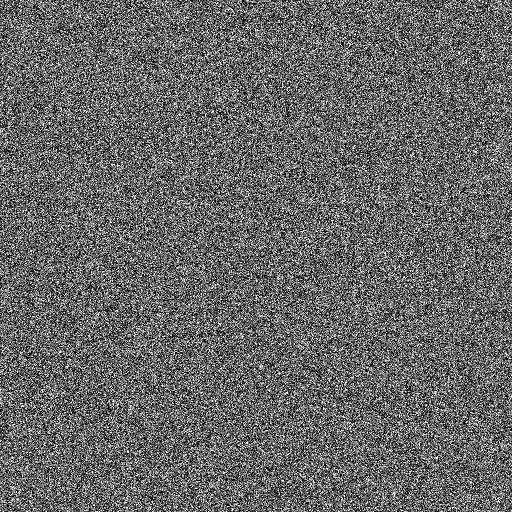
(a1) numbers.RPM	(b1) numbers.RCS	(c1) numbers.ATM	(d1) numbers.SS
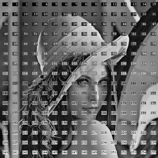
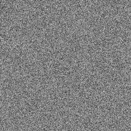
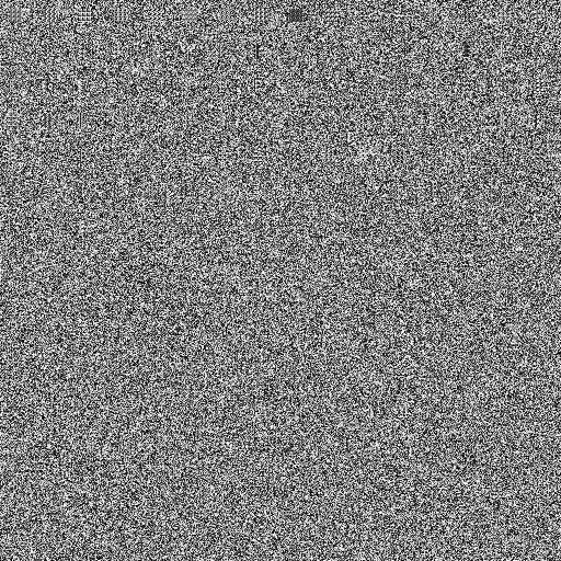
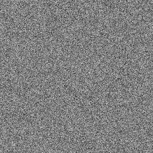
(e1) Original image: numbers.512	(f1) numbers.CBC	(g1) numbers.ECB	(h1) numbers.LME
(a2) ruler.RPM	(b2) ruler.RCS	(c2) ruler.ATM	(d2) ruler.SS
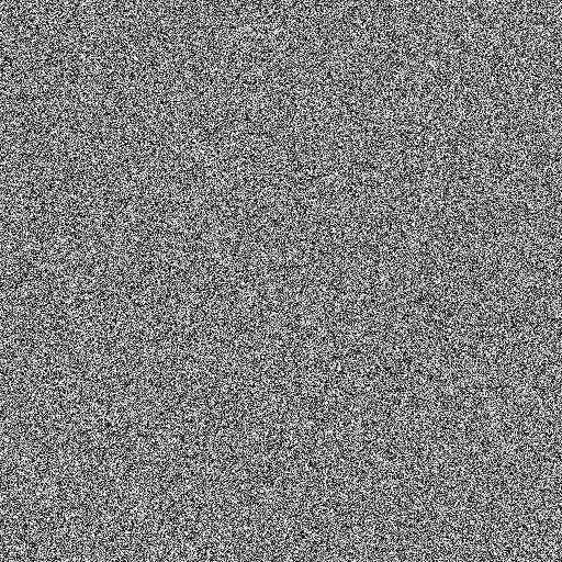
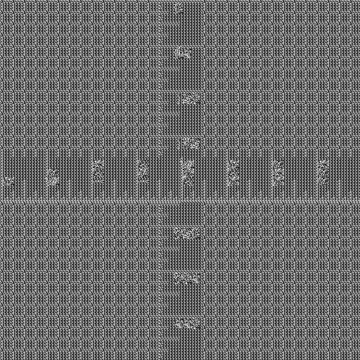
(e2) Original image: ruler.512	(f2) ruler.CBC	(g2) ruler.ECB	(h2) ruler.LME

Figure 1: Shuffled and encrypted images

Evaluation results for these methods are listed in Table III. As one can see, RPM and AES-CBC have their evaluation scores all above 1-$\alpha$=.95. In contrast, none of evaluation scores for the RCS and ATM is above .95 (emphasized by underlines), indicating that one can distinguish their shuffled images from those perfectly shuffled. The scores for these two methods vary greatly for different test images, especially for the ATM, whose IS performance is known to be related to the period of a random Arnold transform. The AES-EBC has good scores for most images but bad scores for highly structured images like ruler.512 and testpat.1k. The SS and LME both have good evaluation scores above .95 indicating that their shuffled or encrypted images are indistinguishable from random-like. Fig. 1 gives sample results of these methods. Once again, the indistinguishability of shuffled or encrypted images from random-like ones are only a necessary condition for a method to be secure. All these results are sufficient to conclude the methods RCS, ATM and ECB are insecure.

VI Conclusion

We introduced a new randomness (quality) evaluation method for IS. It tests whether an image is indistinguishable from a perfectly shuffled one, whose image pixels are i.i.d. everywhere. The proposed method can be used as a prerequisite test to claim an IS or IE method is secure. Simulation results indicate that this method is accurate and effective for quality evaluation for IS and IE methods. Moreover, it can be used as an indicator of quality control. That is, if a shuffled or encrypted image fails to reach the expected evaluation score, it should be re-shuffled or encrypted using another key. Further, the developed method may be useful as a first step in determining whether or not an IE scheme is suitable for a particular cryptographic application. The proposed method is of a constant complexity and can be easily implemented. Thus, it is well suited for practical applications. A MATLAB implementation can be provided on request.

References

- [1] R. Durstenfeld, “Algorithm 235: Random permutation,” Commun. ACM, vol. 7, no. 7, pp. 420–, Jul. 1964.
- [2] G. Chen, Y. Mao, and C. K. Chui, “A symmetric image encryption scheme based on 3d chaotic cat maps,” Chaos, Solitons and Fractals, vol. 21, no. 3, pp. 749–761, 2004.
- [3] “Advanced encryption standard,” Federal Information Processing Standards Publication 197, 2001.
- [4] D. Stinson, Cryptography: Theory and Practice. Chapman & Hall/CRC, 2006.
- [5] “Security requirements for cryptographic modules,” Federal Information Processing Standards Publication 140-2, pp. 800–22, 2001.
- [6] A. Rukhin, J. Soto, J. Nechvatal, M. Smid, E. Barker, S. Leigh, M. Levenson, M. Vangel, D. Banks, A. Heckert, J. Dray, and S. Vo, “A statistical test suite for random and pseudorandom number generators for cryptographic applications,” NIST Special Publication, pp. 800–22, 2010.
- [7] L. Zhao, A. Adhikari, and K. Sakurai, “A new scrambling evaluation scheme based on spatial distribution entropy and centroid difference of bit-plane,” in Digital Watermarking, ser. Lecture Notes in Computer Science. Springer Berlin / Heidelberg, 2011, vol. 6526, pp. 29–44.
- [8] X. Li, “A new measure of image scrambling degree based on grey level difference and information entropy,” in International Conference on Computational Intelligence and Security, vol. 1, dec. 2008, pp. 350–354.
- [9] X. Yu, J. Zhang, H. Ren, S. Li, and X. Zhang, “A new measurement method of iimage encryption,” in Journal of Physics: Conference Series, vol. 48, no. 1. IOP Publishing, 2006, p. 408.
- [10] Y. Tan and W. Zhou, “Image scrambling degree evaluation algorithm based on grey relation analysis,” in International Conference on Computational and Information Sciences, dec. 2010, pp. 511 –514.
- [11] Y. Wu, J. P. Noonan, and S. Agaian, “Npcr and uaci randomness tests for image encryption,” Journal of Selected Areas in Telecommunications (JSAT), pp. 31–38, April 2011.
- [12] Y. Wu, Y. Zhou, G. Saveriades, S. Agaian, J. Noonan, and P. Natarajan, “Local shannon entropy measure with statistical tests for image randomness,” Information Sciences, 2012.
- [13] Z. Li and X. Yang, “A new measure of image scrambling degree based on statistical hypothesis testing,” in International Congress on Image and Signal Processing, vol. 5, oct. 2010, pp. 2409 –2413.
- [14] G. Ye, “Image scrambling encryption algorithm of pixel bit based on chaos map,” Pattern Recognition Letters, vol. 31, no. 5, pp. 347–354, 2010.
- [15] Y. Wu, Y. Zhou, J. Noonan, K. Panetta, and S. Agaian, “Image encryption using the sudoku matrix,” in SPIE Defense, Security, and Sensing, 2010, pp. 77 080P–77 080P.
- [16] Y. Wu, G. Yang, H. Jin, and J. P. Noonan, “Image encryption using the two-dimensional logistic chaotic map,” Journal of Electronic Imaging, vol. 21, no. 1, p. 013014, 2012.