Accuracy of a new hybrid finite element method for solving a scattering Schrödinger equation.

Abstract

This hybrid method (FE-DVR), introduced by Resigno and McCurdy, Phys. Rev. A 62, 032706 (2000), uses Lagrange polynomials in each partition, rather than “hat” functions or Gaussian functions. These polynomials are  discrete variable representation functions, and are.orthogonal under the Gauss-Lobatto quadrature discretization approximation. Accuracy analyses of this method are performed for the case of a one dimensional Schrödinger equation with various types of local and nonlocal potentials for scattering boundary conditions. The accuracy is ascertained by comparison with a spectral Chebyshev integral equation method, accurate to $1:10^{-11}$. For an accuracy of the phase shift of $1:10^{-8}$ The FE-DVR method is found to be $100$ times faster than a sixth order finite difference method (Numerov), is easy to program, and can routinely achieve an accuracy of better than $1:10^{-8}$ for the numerical examples studied.

LABEL:FirstPage1 LABEL:LastPage#1102

I Introduction

The solution of differential equations by means of expansions into discrete variable representation (DVR) basis functions has become very popular since it was first introduced in the early 1960’s DVR1 . A review can be found in the paper by Light and Carrington DVR2 , and generalizations to multidimensional expansions are also under development LITTLE .

Previously the main application of the DVR method was for obtaining bound state energies and wave functions. For this purpose the wave function is expanded into a set of $N$ basis functions, whose expansion coefficients are to be determined. The calculations are of the Galerkin type, namely, the Hamiltonian applied to the wave function is multiplied on the left by each one of the expansion basis functions, and the result is integrated over the full range of the domain of the variable, leading to a set of $N$ linear equations for the expansion coefficients. The integrals to be evaluated are then approximated by discrete sums over the values of the integrand evaluated at the support points times certain weight factors such as in the Gauss quadrature methods NIST .

In the case of the solution of scattering problems the finite element method (FEM) FE has also been developed. In this procedure the radial range is divided into partitions, also called elements, and the solution of the wave equation in each partition is expanded into basis functions such as “hat” functions, Gaussians, or polynomials of a given order, whose expansion coefficients are to be determined. The equations for the expansion coefficients are obtained through a Galerkin procedure, and in many cases the integrals over the basis functions can be done analytically. The continuity of the wave function from one partition to the next is achieved by imposing conditions on the expansion coefficients, as is done for example in Ref. SB . In the more recent DVR methods the basis functions are Lagrange polynomials whose zeros occur at the Lobatto points KOPAL , KRYLOV , in which case the quadrature is denoted as Gauss-Lobatto, and the basis set of functions is denoted as Lagrange-Lobatto. This basis set was first suggested by Manolopoulos and Wyatt MAN , and a extensive review is given in Ref. SFB . The main computational advantage of using DVR basis functions is that the sum mentioned above reduces to only one term, because the product of two different DVR functions vanishes at the support points, and only products between the same DVR functions remain. Furthermore, within the approximation of the Gauss-Lobatto quadrature rule, the basis functions are orthogonal. Hence the procedure leads to a discretized hamiltonian ($N\times N)$ matrix, whose eigenfunctions determine the expansion coefficients and the eigenvalues determine the bound-state energies. There are several types of errors introduced by this method. One is due to the truncation of the expansion of the wave function in terms of basis functions at an upper limit $N,$ another is due to the approximation of the Gauss-Lobatto quadrature described above in terms of discrete sums over the support points. A third error is the accumulation of machine round-off errors. These errors have been examined for bound state energy eigenvalues, WEI , BASEL , LITTLE , SCHN  and it is found that the convergence of the energy with the number $N$ of DVR basis functions is exponential, and the non-orthogonality error becomes small as $N$ increases.

Very recently a combination of the FE and DVR methods has been introduced into atomic physics by Rescigno and McCurdy MCC for quantum scattering calculations . These calculations use the FEM approach but in each partition the basis functions are Lagrange polynomials, and the support points are Gauss- Lobatto. This “hybrid” method, denoted as FE-DVR, is now extensively used for atomic physics calculations, such as for multi electron density distributions in atoms BBB , for photo-ionizing cross sections with fast photon pulses LINHO , HCS , and for atom-atom scattering calculations TMR , to name a few. However, in these works the accuracy of the results was not studied in detail. The FE-DVR method is also used extensively for fluid dynamic calculations since the 1980’s PAT and also in Seismology TROMP , where it is called spectral element method.

The main purpose of the present study is to investigate the accuracy of the FE-DVR method for the scattering conditions, since all the errors described above (the Gauss- Lobatto’s integration error, the truncation errors of the expansions, and the accumulation of round-off errors) are still present. In our study a method of imposing the continuity of the wave function and of the derivative from one partition to the next is explicitly given, and the accuracy is obtained by comparing the results of the FE-DVR calculation for particular solutions of a one dimensional Schrödinger equation with a spectral SPECTRAL Chebyshev expansion method IEM , S-IEM. The accuracy of the latter is of the order of $1:10^{-11},$ as is demonstrated in Appendix A. In our present formulation of the FE-DVR the so-called bridge functions used in references MCC -TMR in order to assure the continuity of the wave function are not used, but are replaced by another method.

In section II the FE-DVR method is described, in section III the accuracy is investigated by means of numerical examples, and section IV contains the summary and conclusions. Appendix $A$ contains a short review of the S-IEM method, in appendix $B$ an estimate of the accumulation of errors is presented, and in Appendix $C$ some accuracy properties of the finite difference Numerov (or Milne’s) method are presented.

II The  FE-DVR method

The FE-DVR version of the finite element method differs from the conventional FEM in that the basis functions for the expansion of the solution $\psi(x)$ in each partition are $N$ “discrete variable representation” (DVR) functions, which in the present case are Lagrange polynomials $\ell_{i}(x)$, $i=1,2,..N$ of a given order $N-1,$

$$\ell_{i}(x)={\displaystyle\prod_{k=1}^{N}}\frac{(x-x_{k})}{(x_{i}-x_{k})},~{}~{}k\neq i$$ (1)

defined for example in Eq. $(25.2.2)$ of Ref. AS , and in section 3.3(i) of Ref. NIST . These functions are widely used for interpolation procedures and are described in standard computational textbooks. This FE and DVR combination was introduced in Ref. MCC , and has the advantage that integrals involving these polynomials amount to sums over the functions evaluated only at the support points. In the present case the support points are Lobatto points $x_{j}$ and weights $w_{j}$, $j=1,2,..N,$ defined in Eq. $(25.4.32)$ of Ref. AS , in terms of which a quadrature over a function $f(x)$ in the interval $[-1,+1]$ is approximated by

$$\int_{-1}^{+1}f\left(x\right)dx\simeq\sum_{j=1}^{N}f(x_{j})w_{j}.$$ (2)

If $f$ is a polynomial of degree $\leq 2N-3$ then Eq. (2) will be exact. This however is not the case for the product of two Lagrange polynomials $\ell_{i}(x)\ell_{j}(x),$ a polynomial of order $2(N-1).$ In the Gauss-Lobatto quadrature approximation KOPAL , KRYLOV , given by the right hand side of Eq. (2), these Lagrange polynomials are orthogonal to each other, but they are not rigorously orthogonal BASEL because the left hand side of Eq. (2) is not equal to the right hand side. If the integral limits are different from $\pm 1$, such as $\int_{a}^{b}f(r)dr$ then the variable $r$ can be scaled to the variable $x.$ Our method differs from that of Ref. MCC in that we do not use their “bridge” functions, but rather insure continuity of the solution and its derivative from one partition to the next by using only the Lagrange functions. Since the Lobatto points are not evenly spaced, expansion (2) converges uniformly, which is a general feature of spectral methods SPECTRAL . A further $DVR$ advantage is that the Gauss-Lobato approximation of the integral

$$\int_{-1}^{1}\ell_{i}(x)f\left(x\right)\ell_{j}(x)dx\simeq\delta_{i,j}w_{j}f(x_{i})$$ (3)

is diagonal in $i,j$ and is given by only one term. The convolution

$$\int_{-1}^{1}\ell_{i}(x)\int_{-1}^{1}K\left(x,x^{\prime}\right)\ell_{j}(x^{\prime})dx^{\prime}\ dx\simeq w_{i}w_{j}K(x_{i},x_{j})$$ (4)

is also approximated by one non-diagonal term only, which is a marked advantage for solving nonlocal or coupled channel Schrödinger equations. The kinetic energy integral can be expressed in the form

$$\int_{-1}^{1}\ell_{i}(x)\frac{d^{2}}{dx^{2}}\ell_{j}(x)dx=-\int_{-1}^{1}\ell_{i}^{\prime}(x)\ell_{j}^{\prime}(x)dx+\delta_{i,N}\ell_{j}^{\prime}(1)-\delta_{i,1}\ell_{j}^{\prime}(-1)$$ (5)

after an integration by parts. In the above the prime denotes $d/dx.$ The integral on the right hand side of this equation can be done exactly with the Gauss-Lobatto quadrature rule (2), since the integrand is a polynomial of order $2N-4$, that is less than the required $2N-3.$

For the case of a local potential $V$ with angular momentum number $L=0$ the equation to be solved is

$$\left(\frac{d^{2}}{dr^{2}}+k^{2}\right)\psi(r)=V(r)\psi(r),$$ (6)

and for a nonlocal potential $K$, the term $V(r)\psi(r)$ is replaced by $\int_{0}^{\infty}K(r,r^{\prime})\psi(r^{\prime})dr^{\prime}.$ The wave number $k$ is in units of $fm^{-1}$ and the potential $V$ is in units of $fm^{-2}$, where quantities in energy units are transformed to inverse length units by multiplication by the well known factor $2m/\hslash^{2}.$ In the scattering case the solutions $\psi(r)$ are normalized such that for $r\rightarrow\infty$ they approach

$$\psi(r)\rightarrow\sin(kr)+\tan(\delta)\cos(kr),$$ (7)

and with that normalization one finds

$$\tan(\delta)=-\frac{1}{k}\int_{0}^{\infty}\sin(kr)\ V(r)\ \psi(r)dr,$$ (8)

as is well known LANDAU .

The FE-DVR procedure is as follows. We divide the radial interval into $N_{J}$ partitions (also called elements in the finite element calculations FE ), and in each partition we expand the wave function into $N$ Lagrange functions $\ell_{i}(r),i=1,2,..N$

$$\psi^{(J)}(r)=\sum_{i=1}^{N}c_{i}^{(J)}\ell_{i}(r),~{}~{}\ b_{1}^{(J)}\leq r\leq\vskip 12.0pt plus 4.0pt minus 4.0ptb_{2}^{(J)},$$ (9)

The starting and end points of each partition are denoted as $b_{1}^{(J)}$ and $b_{2}^{(J)}$, respectively. We define the value and the derivative of the wave function at the end point of the previous partition as

$$\psi^{(J-1)}(b_{2}^{(J-1)})=c_{N}^{(J-1)},$$ (10)

where $c_{N}^{(J-1)}$ is the last coefficient of the expansion (9) of $\psi^{(J-1)}$, and

$$A^{(J-1)}\equiv\frac{d}{dr}\psi^{(J-1)}(b_{2}^{(J-1)})=\sum_{i=1}^{N}c_{i}^{(J-1)}\ell\ _{i}^{\prime}(b_{2}^{(J-1)}),$$ (11)

respectively, where $\ell\ _{i}^{\prime}(r)=d\ell_{i}(r)/dr.$ The result (10) follows from the fact that that $\ell_{i}(b_{2})=0$ for $i=1,2,..N-1$, and $\ell_{N}(b_{2})=1$. For the first partition we arbitrarily take a guessed value of $A^{(0)}$ for the non-existing previous partition, and later renormalized the whole wave function by comparing it to a known value. That is equivalent to renormalizing the value of $A^{(0)}$. In finite element calculations continuity conditions of the wave function from one partition to the next are also imposed. However, the method described below applies specifically to the case that the basis functions in each element are of the DVR type, rather than general polynomials of a given order SB .

By performing the Galerkin integrals of the Schrödinger Eq. over the $\ell_{i}$ in each partition $J$

$$\langle\ell_{i}(T+V-k^{2})\psi^{(J)}\rangle =$$ (12)

$$\int_{b_{1}^{(J)}}^{b_{2}^{(J)}}\ell_{i}(r)(T+V-k^{2})\psi^{(J)}(r)dr =0,~{}~{}\ i=1,2,..N$$ (13)

we obtain a homogeneous matrix equation in each partition for the coefficients $c_{i}^{(J)},$ $i=1,2,..N$

$$M^{(J)}\ \vec{c}^{(J)}=0,$$ (14)

where $\vec{c}^{(J)}$ represents the ($N\times 1)$ column vector of the coefficients $c_{i}^{(J)},$ and where the matrix elements of $M$ are given by $M_{ij}=\langle\ell_{i}(T+V-k^{2})\ell_{j}\rangle.$ Here $T=-d^{2}/dr^{2}.$ The continuity conditions are imposed by transforming the homogeneous equation (14) of dimension $N$ into an inhomogeneous equation of dimension $N-2$ whose driving terms are composed of the function $\psi$ and $d\psi/dr$ evaluated at the end of the previous partition. These conditions are given by

$$c_{1}^{(J)}=c_{N}^{(J-1)}$$ (15)

where use has been made of $\ell_{i}(b_{1})=0$ for $i=2,..N$, and $\ell_{1}(b_{1})=1,$ and

$$\frac{d\ \psi^{(J-1)}(b_{2}^{(J-1)})}{dr}=\sum_{i=1}^{N}c_{i}^{(J)}\ell\ _{i}^{\prime}(b_{1}^{(J)})=A^{(J-1)}.$$ (16)

These two conditions can be written in the matrix form

$$F_{11}\alpha+F_{12}\beta=\gamma$$ (17)

where

$$F_{11}=\begin{pmatrix}1&0\\ \ell_{1}^{\prime}&\ell_{2}^{\prime}\end{pmatrix}_{b_{1}^{(J)}}^{(J)};~{}~{}F_{12}=\begin{pmatrix}0&0&\cdots&0\\ \ell_{3}^{\prime}&\ell_{4}^{\prime}&\cdots&\ell_{N}^{\prime}\end{pmatrix}_{b_{1}^{(J)}}^{(J)},$$ (18)

where

$$\alpha=\begin{pmatrix}c_{1}\\ c_{2}\end{pmatrix}^{(J)},$$ (19)

where

$$\beta=\begin{pmatrix}c_{3}\\ c_{4}\\ \vdots\\ c_{N}\end{pmatrix}^{(J)},$$ (20)

and where

$$\gamma=\begin{pmatrix}c_{N}\\ A\end{pmatrix}^{(J-1)}.$$ (21)

With that notation Eq. (14) can be written in the form

$$\begin{pmatrix}M_{11}&M_{12}\\ M_{21}&M_{22}\end{pmatrix}\begin{pmatrix}\alpha\\ \beta\end{pmatrix}=0,$$ (22)

where the matrix $M^{(J)}$ has been decomposed into four submatrices $M_{11},M_{12},M_{21}$, and $M_{22},$ which are of dimension $2\times 2,2\times(N-2),(N-2)\times 2,$ and $(N-2)\times(N-2),$ respectively. The column vector $\alpha$ can be eliminated in terms of $\beta$ and $\gamma$ by using Eq. (17),

$$\alpha=F_{11}^{-1}(-F_{12}\beta+\gamma)$$ (23)

and the result when introduced into Eq. (22) leads to an inhomogeneous equation for $\beta$

$$(-M_{21}F_{11}^{-1}F_{12}+M_{22})\beta=-M_{21}F_{11}^{-1}\gamma.$$ (24)

Once the vector $\beta$ is found from Eq. (24), then the components of the vector $\alpha$ can be found from Eq. (23), and the calculation can proceed to the next partition.

If one expresses the inverse of $F_{11}$ analytically

$$F_{11}^{-1}=\begin{pmatrix}1&0\\ -\ \frac{\ell_{1}^{\prime}}{\ell_{2}^{\prime}}&\frac{1}{\ell_{2}^{\prime}}\end{pmatrix}.$$ (25)

then one finds

$$F_{11}^{-1}\gamma=\begin{pmatrix}c_{N}^{(J-1)}\\ -\ \frac{\ell_{1}^{\prime}}{\ell_{2}^{\prime}}c_{N}^{(J-1)}+\frac{A^{(J-1)}}{\ell_{2}^{\prime}}\end{pmatrix}$$ (26)

and

$$F_{11}^{-1}F_{12}=\begin{pmatrix}0&0&\cdots&0\\ \frac{\ell_{3}^{\prime}}{\ell_{2}^{\prime}}&\frac{\ell_{4}^{\prime}}{\ell_{2}^{\prime}}&\cdots&\frac{\ell_{N}^{\prime}}{\ell_{2}^{\prime}}\end{pmatrix}.$$ (27)

Inserting (25) into (23) one finds that $c_{1}^{(J)}=c_{N}^{(J-1)}$, but $c_{2}^{(J)}$ is a function of $c_{N}^{(J-1)}$, $A^{(J-1)},$ and the vector $\beta.$

III Accuracy

We have tested the accuracy for cases with angular momentum $L=0$ for two local potentials $V_{M}$ and $V_{WS},$ shown in Fig. 1, and for a nonlocal potential $K(r,r^{\prime})$ of the Perey-Buck type PB . Potential $V_{M}$ is of a Morse type with a repulsive core near the origin, given by

$$V_{M}(r)=6\exp(-0.3\ r+1.2)\times\left[\exp(-0.3\ r+1.2)-2\right].$$ (28)

and $V_{WS}$  is a short-ranged simple Woods-Saxon potential given by

$$V_{WS}(r)=-3.36/\{1+\exp[(r-3.5)/0.6]\}.$$ (29)

The coefficients $6$ and $-3.36$ are in units of $fm^{-2}$, the distances $r$ are in units of $fm$, and all other factors are such that the arguments of the exponents are dimensionless. These potentials are shown in Fig. 1, and the respective wave functions are shown in Fig. 2.

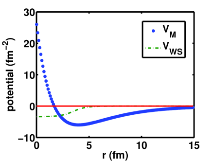
Figure 1: (Color on line) Potentials Morse $V_{M}$  and Woods Saxon $V_{WS}$ as a function of radial distance $r$. These potentials are given by Eqs. (28) and (29), respectively.

The choice of these potentials is motivated by the difference in the degree of computational difficulty that they offer in the solution of the Schrödinger equation. Potential $V_{WS}$ has no repulsive core near the origin and is of short range. Hence the corresponding wave function does not have large derivatives near the origin, and needs not to be calculated out to distances larger than $20$ $fm$, where the potential is already negligible, of the order or $10^{-11}$. By contrast, neither of these two features apply for the case of $V_{M}$. In order to obtain an accuracy of $1:10^{-11}$ the wave function has to be calculated out to $100\ fm$, as is indeed done in the calculation of the bench mark S-IEM solution, and the repulsive core near the origin is more difficult to treat. The nonlocal potential $K$ is described in Eq. ($3$) of Ref. RPB together with the Appendix of Ref. PB . The accuracy of the corresponding wave function obtained with the S-IEM method for this nonlocal potential is illustrated in Fig. $7$ of Ref. RPB . For the nonlocal case only one partition is used in the FE-DVR method, that extends from $r=0$ to $R_{\max},$ but in view of Eq. (4), the calculation is very efficient.

In order to ascertain the accuracy of the FE-DVR method, the solutions of Eq. (6) are compared with the solutions obtained by the spectral integral equation method (S-IEM) IEM , whose accuracy is $1:10^{-11},$ as described in Appendix A. The numerical FE-DVR solutions are first normalized by comparison with the S-IEM solutions at one chosen radial position near the origin, and the error of the normalized FE-DVR function is determined by comparison with the S-IEM function at all other radial points $r.$ Since the S-IEM function depends on the values of the potential at all points $[0\leq r\leq R_{\max}],$ the S-IEM calculation has to be carried out to a distance $R_{\max}$ large enough so that the contribution from $V(r\geq R_{\max})$ is smaller than the desired accuracy of the S-IEM   solution. The same is not the case for the FE-DVR solutions $\psi_{FE-DVR}(r),$ since the un-normalized solution depends only on the potentials for distances less than $r$. However, if the normalization of the wave function (7) is to be accomplished by matching it to $\sin(kr)$ and $\cos(kr)$ at $R_{\max}$ in the asymptotic region, then the numerical errors that accumulated out to $R_{\max}$ will affect the wave function at all distances. These errors can be avoided by an iterative procedure for the large distance part of the wave function, as will be described in a future publication RAW-ITER .

The results for potentials $V_{WS}$ and $V_{M}$ are shown figures 3 and 4, respectively. In both cases the error of the wave function starts with $10^{-11}$ at the small distances, and increases to $10^{-10}$ as the distance increases, due to the accumulation of various errors. The accuracy for the nonlocal potential $K$ is shown in Fig. 5. The accuracy of the integral (8), for a fixed size of all partitions as a function of the number $N$ of Lobatto points in each partition, is shown in Fig. 6, where the open circles represent an upper limit of the estimated accuracy as developed in Appendix B, of order $(N-2)^{3}.$ This figure is important because it shows the nearly exponential increase of accuracy as $N$ increases, until the accumulation of errors overwhelms this effect once the value of $N$ increases beyond a certain value, $20$ for the case of Fig. 6. The accuracy of the integral (8) for a fixed number $N$ per partition, but for several different partition sizes, is displayed in Fig. 9. This figure shows that the accuracy decreases exponentially with the size of the partition, which can be interpreted as an exponential increase of the accuracy with the number of Lobatto points in each partition of fixed length.

Finally, the FE-DVR computing time as a function of the number $N$ of Lobatto points in each partition is displayed in Fig. 8, where it is also compared with an estimate described in Appendix $B$ of the number of floating point operations expected. According to this estimate, the time per floating point operation turns out to be $\simeq 10^{-8}$ in a MATLAB computation performed on a desktop using an Intel TM2 Quad, with a CPU Q 9950, a frequency of 2.83 GHz, and a RAM of 8 GB. The dashed line represents the total time required for a comparable S-IEM computation. That comparison shows that the FE-DVR method can be substantially faster than the S-IEM even though the former has many more support points, depending on the radial range and on the accuracy required. Further details are given in Table 2 in Appendix A.

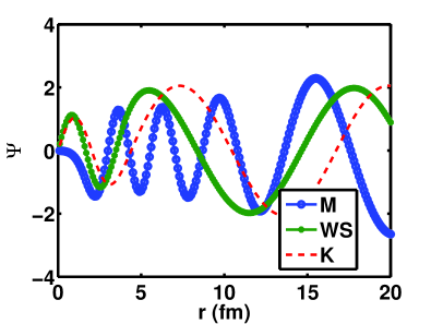
Figure 2: (Color on line) The wave functions for the local potentials $V_{M}$ and $V_{WS},$ and for the nonlocal potential $K$, described in the text. The wave number is $k=0.5$ $fm^{-1}$ and the potentials $V_{M}$ and $V_{WS}$ are illustrated in Fig. 1.

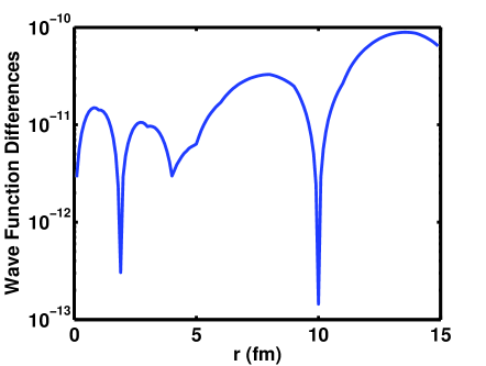
Figure 3: (Color on line) Accuracy of the FE-DVR solution of the Schrödinger Eq. for the Woods Saxon potential $V_{WS}$ displayed in Fig. 1. The wave number is $k=0.5\ fm^{-1}$, the size of each partition is $1.fm$, and there are $20\$Lobatto points per partition. The graph shows the accuracy of the wave function $\psi$ by displaying the absolute value of the difference between the FE-DVR and the S-IEM wave functions. The latter is deemed accurate to $1:10^{-11}$.

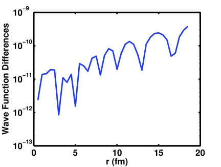
Figure 4: (Color on line) The accuracy of the FE-DVR wave function for the potential $V_{M}$ as obtained by comparison with the S-IEM result. The latter is accurate to $1:10^{-11}.$ The wave number is $k=0.5\ fm^{-1},$ the number of Lobatto points per partition is $20$, the size of each partition is $1\ fm.$

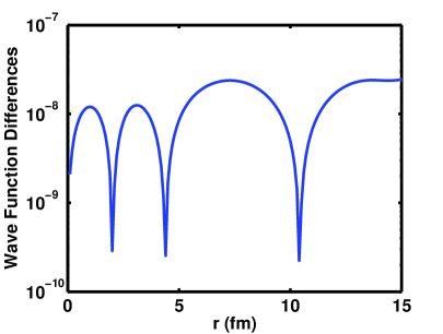
Figure 5: (Color on line) Same as Fig. 3 for the nonlocal Perey-Buck potential $K(r,r\prime)$. The wave number is $k=0.5fm^{-1}$, only one partition was used in the full radial interval from $0$ to $15$ $fm$ using a total of $130$ Lobatto grid points. The accuracy of $10^{-8}$ is consistent wth the estimate made in Eq. (33) in Appendix B.

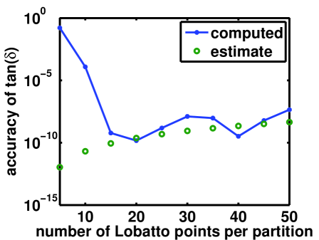
Figure 6: (Color on line) Accuracy of the integral $\int_{0}^{100}\sin(kr)\ V_{M}(r)\ \psi(r)\ dr,$ obtained with the FE-DVR method as a function of the number of Lobatto points in each partition. The length of each partition is $1.0\ fm$, the number of partitions is $100$. The potential is $V_{M}$, the wave number is $k=0.5\ fm^{-1}$, the accuracy is obtained by comparisom with the S-IEM result which is accurate to $1:10^{-11}$. The open circles represent an estimate of the upper bound for the accumulation of roundoff errors, given by Eq. (30) in Appendix B.

A comparison between the FE-DVR and a finite difference sixth order Numerov method  of the accuracy of $\tan(\delta)$ is illustrated in Fig. 7.

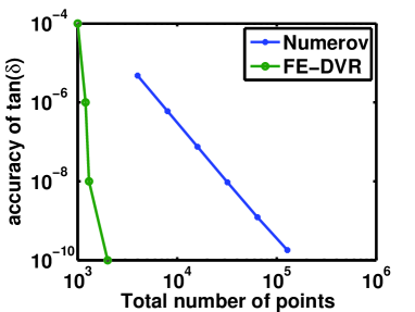
Figure 7: (Color on line) This accuracy comparison for $\tan(\delta)$ is performed for the potential $V_{M}$ and $k=0.5\ fm^{-1}$ in the radial interval $[0,100fm]$. The partition sizes in the FE-DVR method have a length of $1\ fm$ each, and the number of Lobatto points in each partition is given by $1/100\ th$ of the total number of points. Numerov is a 6th order finite difference method with equidistant points, as described in Appendix C.

This comparison shows that for an accuracy of $\tan(\delta)$ of $\simeq 10^{-8}$, the FE-DVR method requires $15$ times fewer meshpoints, and is approximately $100$ times faster than the Numerov method. More details are presented in Appendix C.

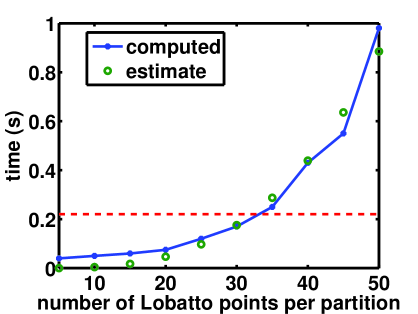
Figure 8: (Color on line) The computing time in MATLAB for the calculations described in Fig. 6. The estimate is given by Eq. (30), with the factor $10^{-16}$ replaced by $2\times 10^{-8}.$ The latter represents the time for each floating point operation. The dashed line represents the computing time for the S_IEM calculation, described in Fig. 6.

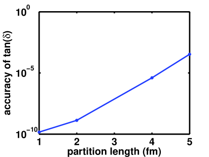
Figure 9: (Color on line) Accuracy of the integral $\int_{0}^{100}\sin(kr)\ V_{M}(r)\ \psi(r)\ dr$, Eq. (8), as a function of the length of each partition, into which the radial interval $[0,100\ fm]$ is divided. The total number $N=20$ of Lobatto points in each partition is kept constant. The conditions are the same as in Fig. 6. This figure shows that the accuracy decreases exponentially with the size of the partition. For $20$ partitions the computation time is $0.060$ s, for $100$ partitions it is $0.075$ s.  

IV Summary and Conclusions

The accuracy of a hybrid finite element method (FE-DVR) has been examined for the solution of the one dimensional Schrödinger equation with scattering boundary conditions. This method  MCC uses as basis functions the discrete variable representation Lagrange polynomials $\ell_{i}(r)$, $i=0,1,2,..N,$ on a mesh of $N$ Lobatto support points. The accuracy of the FE-DVR method is obtained by comparison with a spectral method S-IEM, whose accuracy is of the order of $1:10^{-11}$. An important advantage of a discrete variable representation basis is the ease and accuracy with which integrals can be performed using a Gauss-Lobatto integration algorithm that furthermore render the matrix elements $\langle\ell_{i}(V-E)\ell_{j}\rangle$ diagonal. This feature permits one to easily solve the Schrödinger Eq. also in the presence of nonlocal potentials with a kernel of the form $K(r,r^{\prime}),$ as is demonstrated in one of our numerical examples. Another advantage is that the Galerkin matrix elements of the kinetic energy operator $T$ need not be recalculated anew for each partition because they are the same in all partitions to within a normalization factor that only depends on the size of the partition. A further advantage is that the convergence of the expansion (9) with the number $N$ of basis functions is exponential, in agreement of what it is the case for bound state finite element calculations with Lobatto discretizations BASEL . A possible disadvantage may be that if the number of the Lagrange polynomials in each partition is very large and/or the number of partitions is large, as is the case for long ranged potentials, then the accumulation of roundoff and algorithm errors may become unacceptably large.

In summary, for scattering solutions of the Schrödinger equation the accuracy of the FE-DVR method increases exponentially with the number of Lagrange polynomials in each partition until the accumulation of roundoff and truncation errors overwhelm the result. The FE-DVR can easily achieve an accuracy of the order of $10^{-10}$ for the scattering phase shifts for either local or nonlocal short ranged potentials; it is less complex than the spectral S-IEM method but is comparable in the amount of computing time; and, in addition, it is substantially more efficient than a finite difference Numerov method. The latter result is demonstrated by the fact that the FE-DVR was found to be a hundred times faster than the Numerov for an accuracy of $10^{-8}$ of the scattering phase shift.

Acknowledgements: One of the authors (GR) is grateful to Professor McCurdy for a stimulating conversation on the use of Lagrange polynomials in finite element calculations.

Appendix A: the S-IEM method

A version of the spectral method employed here was developed recently IEM . It consists in dividing the radial interval into partitions of variable size, and obtaining two independent solutions of the Schrödinger Eq. (6) in each partition , denoted as $Y(x)$ and $Z(x)$. These solutions are obtained by transforming Eq. (6) into an equivalent Lippmann-Schwinger integral equation (L-S) and solving the latter by expanding the solution into Chebyshev functions, mapped to the interval $[-1,+1]$. The corresponding discretized matrices are not sparse, but are of small dimension equal to the number of Chebyshev points per partition. The solution $\psi$ in each partition is obtained by a linear combination of the two independent functions $Y(x)$ and $Z(x)$, with coefficients that are determined from the solution of a matrix equation of dimension twice as large as the number of partitions, but the corresponding matrix is sparse. Details are given in Ref. IEM , and a pedagogical version is found in Ref. STRING .

One of the features of the S-IEM method is that the size of each partition is adaptively determined such that the accuracy of the functions $Y(x)$ and $Z(x)$ is equal or better than a pre-determined accuracy parameter $tol$, which in the present case is $tol=10^{-12}.$ In the region where the potential $V$ is small the corresponding partition size is large. When the number of Chebyshev expansion functions $N$ per partition is large the size of the partitions is correspondingly large. As is illustrated in Fig. 10 when $N$ is increases from $17$ to $33$ the number of partitions decreases from $29$ to $6$, yet the accuracy of the respective wave functions is approximately the same, $1:10^{-11},$ and the computing time is also approximately the same, $0.2s.$

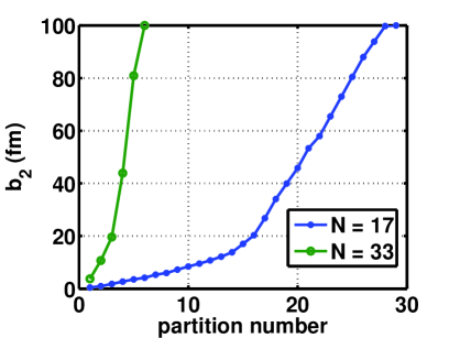
Figure 10: (Color on line) The partition distrtibution for the S-IEM method in the radial interval $[0,100\ fm]$. for two different numbers $N$ of the Chebyshev expansion functions in each partition. The end point $b_{2}$ of each partition is shown on the vertical axis, and the corresponding partition number is shown on the horizontal axis. The potential is $V_{M}$ , and the wave number is $k=0.5\ fm^{-1}$. The accuracy parameter $tol$ in each partition is $10^{-12}.$ The computation time for each case is approximately the same, $0.2\ s,$and the accuracy of the wave function in both cases is the same, $1:10^{-11}.$

For the present S-IEM benchmark calculations the value of $N$ is $17$, and for the case of $V_{M}$ the maximum value of $r$ is $100\ fm.$ Such a large value is required because the potential decays slowly with distance and becomes less in magnitude than $5\times 10^{-12}$ only beyond $r=100\ fm$. Had the potential been truncated at a smaller value of $r,$ then the truncation error would have propagated into all values of the wave function and rendered it less accurate. The accuracy of the S-IEM wave function can be seen from Fig. 11, which compares two S-IEM wave functions with accuracy parameters $tol=10^{-11}$ and $10^{-12}$, respectively. The result is that the accuracy of the IEM wave function for $N=17$ and $R_{\max}=100fm$ and $tol=10^{-11}$ is $4\times 10^{-11},$ and that for $tol=10^{-12}$ the accuracy is better than $10^{-11}.$

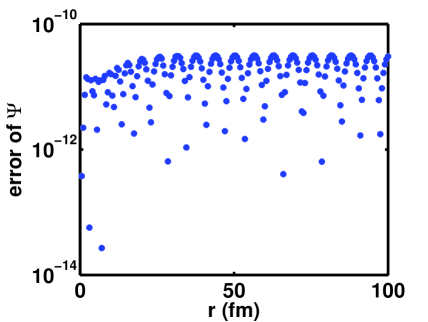
Figure 11: (Color on line) The y-axis illustrates the absolute value of the difference between two S-IEM wave functions, calculated with accuracy parameters $tol=10^{-11}$ and $10^{-12},$ respectively, for potential $V_{M}$ and $k=0.5\ fm^{-1}$. This difference is less than $4\times 10^{-11}$ for all values of $r.$

The wave functions are normalized such that their asymptotic value is given by Eq. (7). The corresponding values of $\tan(\delta)$, Eq. (8), for potentials $V_{M}$ and $V_{WS}$ and a wave number $k=0.5\ fm^{-1}$ are $2.6994702502$ and $-1.7107344227$, respectively. Table 1 shows the number of partitions, the accuracy of $\tan(\delta)$, and the computing time of the S-IEM method for various tolerance parameters inputted into the code for the potential $V_{M},$ with $k=0.5.$ The number of Chebyshev polynomials in each partition is $17$, the total number of points displayed in the third column is equal to $17$ times the number of partitions. The error of $\tan(\delta)$ is obtained by comparing the value of tan$(\delta)$ for a particular tolerance parameter with the value obtained for $tol=10^{-12}.$

$Tol.$	$Part^{\prime}ns$	$Points$	$Err[$tan$(\delta)]$	$time\ (s)$
$10^{-12}$	$37$	$629$	$-$	$0.178$
$10^{-10}$	$25$	$425$	$4.6\times 10^{-12}$	$0.181$
$10^{-8}$	$17$	$289$	$7.7\times 10^{-11}$	$0.171$
$10^{-6}$	$11$	$187$	$5.2\times 10^{-7}$	$0.165$
$10^{-4}$	$7$	$119$	$2.8\times 10^{-4}$	$0.162$
$10^{-2}$	$5$	$85$	$6.5\times 10^{-2}$	$0.161$

Table 1: Accuracy and computing time for the S-IEM method

For the case of a nonlocal potential $K$ the division  of the radial interval into partitions is not made because the effect of the nonlocal potential would extend into more than one partition, making the programming more cumbersome. For the case of a kernel $K(r,r^{\prime}),$ described in Ref. RPB , the accuracy of the S-IEM result RPB is also good to $1:10^{-11},$ as is shown in Fig. 7 of Ref. RPB .

For comparison with the S-IEM method some characteristics of the FE-DVR method are shown in Table 2. The potential and the wave number is the same as in Table 1, the radial interval $[0,100\ fm]$ is divided into $100$ partitions of length of $1\ fm$ each, and the number of Lobatto points per partition in all partitions is the same but is progressively varied from $20$ to $7,$ as shown in the table. If one compares the entries in table 1 with those in 2 that correspond to approximately the same accuracy of $10^{8}$ for tan$(\delta)$ one notices that the FE-DVR method needs approximately 7 times more support points than the S-IEM, yet the computing time is between 2 and 3 times less. This remark attests to the efficiency of the FE-DVR method.

$N\ of\ Pts.$	$err[$tan$(\delta)]$	$time(s)$
$2000$	$10^{-10}$	$0.075$
$1300$	$10^{-8}$	$0.050$
$1200$	$10^{-6}$	$0.047$
$1000$	$10^{-4}$	$0.045$
$700$	$10^{-2}$	$0.042$

Table 2: Accuracy and computing time for the FEM-DVR method

Appendix B: The round off errors in the FE-DVR method.

The notation is as follows: $N$ is the number of Lobatto points in each partition, which is also equal to the number of Lagrange polynomials in each partition, and $N_{p}$ is the number of partitions. The largest contribution to the roundoff errors is expected to arise from the solution of Eq. (24) for the $N-2$ expansion coefficients. This equation is of the type $\bar{M}\beta=b,$ where $\beta$ is the column vector of the $N-2$ expansion coefficients and $\bar{M}$ is a matrix of dimension $N-2,$ whose solution requires $4\times(N-2)^{3}$ floating point operations. For the case that the floating point roundoff error of the computer is $\varepsilon$ and that the errors accumulate linearly, an upper bound for the total error $\varepsilon_{T}$ is

$$\varepsilon_{T}\approx 4\ast N_{P}(N-2)^{3}\varepsilon.$$ (30)

For $N_{p}=100$ and for $\varepsilon=10^{-16},$ which is the value for the calculations done in MATLAB, one obtains an upper bound for the values of $\varepsilon_{T}$ that are plotted in Fig. 6 as a function of $N$

$$\varepsilon_{T}\approx 4\times 10^{-14}(N-2)^{3}\varepsilon.$$ (31)

The floating point error that occurs in the calculation of the Lagrange functions $\ell_{i}(x)$ is much smaller. The numerator contains $N$ factors $x-x_{i}$ , each of which can be written as $\Delta_{i}+\varepsilon$, where $\Delta_{i}$ is proportional to the length of each partition. Hence the error of the product is $\approx\Delta^{N}+N\Delta^{N-1}\varepsilon,$ where $\Delta$ is an average value of the $x-x_{i}.$ A similar argument holds for the denominator and if the error of the numerator adds linearly to the error of the denominator, then an upper bound for the total error of a Lagrange function is $\simeq 2N\varepsilon/\Delta$. This is much less than the error in Eq. (30).

For the case of the nonlocal calculation the conditions above are different. There is only one partition of length $L=15\ fm,$ the number of Lobatto points is $130$, and the order of each polynomial $\ell(r)$ is $129.$ The error in the calculation of the Lagrange polynomials, or their derivatives at each meshpoint, is $\leq\ 2(N-1)\varepsilon/\Delta$. Since the error in the calculation of the matrix element of $(d^{2}/dr^{2})$ has $N$ terms according to Eq. (5) that could lead to an error of $\simeq 2N(N-1)\varepsilon/\Delta,$ assuming that all $\varepsilon$ errors add linearly. The solution of of Eq. (24) requires $4(N-2)^{3}$ operations and thus an upper bound of the total linear accumulation of $\varepsilon$ errors is

$$\simeq 2N(N-1)(\varepsilon/L)4(N-2)^{3}=1.8\times 10^{-6}.$$ (32)

Since the $\varepsilon$ errors do not accumulate linearly, the expected upper bound for the error could be

$$\leq 2(N-1)(\varepsilon/L)4(N-2)^{3}=1.4\times 10^{-8}.$$ (33)

The above estimate is consistent with the accuracy found numerically in Fig. 5.

Appendix C: Comparison with a finite difference method.

The finite difference method used for this comparison is Milne’s corrector method, also denoted as the Numerov method, given by Eq. 25.5.21 in Ref. AS . In this method the error of the propagation of the wave function from two previous points to the next point is of order $h^{6},$ where $h$ is the radial distance between the consecutive equispaced points. The calculation is done for the potential $V_{M}$ and for $k=0.5\ fm^{-1}$ as follows.

A value of $h$ is selected and the Milne wave function is calculated starting at the two initial points $r=h$ and $r=2h$ by a power series expansion of the wave function for the potential $V_{M}$. The values of the wave function for the additional points $3h,4h,...$are obtained from Milne’s method out to the point $r=20fm.$ The wave function is normalized to the S-IEM value at $r=2\ fm$, and the error at $r=18\ fm$ is obtained by comparison with the S-IEM value at that point. The result for a sequence of $h$ values is illustrated in Fig. 12.

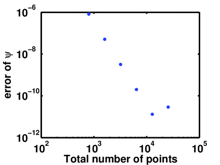
Figure 12: (Color on line) The error of the Numerov wave function at $r=18\ fm,$ as a function of the number $N$ of meshpoints in the interval $[0,20fm]$. The distance $h$ between points is $20/N$. For each $h$ the wave function is normalized to the S-IEM wave function at $r=2\ fm.$ The wave number is $k=0.5\ fm^{-1}$, the potential is $V_{M}.$

For each value of $h$ the wave function is calculated out to $r=100$ $fm$ by Numerov’s method, and the integral (8) is calculated by the extended Simpson’s rule, given by Eq. (25.4.6) in Ref. AS . The error is determined by comparison with the S-IEM result $2.6994702502$ for $\tan(\delta)$. A comparison with the FE-DVR method is shown in Fig. 7 and Table 3 displays the ratio  Numerov/FE-DVR of the total number of points and of the time of the two methods for two accuracies of $\tan(\delta).$

$accuracy\$tan$(\delta)$	$ratio\ of\ N\ of\ Pts$	$time\ ratio$
$10^{-6}$	$\simeq 1$	$20$
$10^{-8}$	$15$	$100$

Table 3: The Numerov/FE-DVR ratio of the required total number of meshpoints and the respective computational times

. More detail of the error and the computing time for the Numerov method is displayed in Table 4.

$N\ of\ Pts.$	$err[$tan$(\delta)]$	$time(s)$
$12800$	$1.23\times 10^{-9}$	$51$
$6400$	$9.41\times 10^{-9}$	$5.8$
$3200$	$7.50\times 10^{-8}$	$2.1$
$1600$	$5.99\times 10^{-7}$	$1.0$
$800$	$4.76\times 10^{-6}$	$0.72$

Table 4: Accuracy and computing time for the Numerov method

. The calculation is done in MATLAB performed on a desktop using an Intel TM2 Quad, with a CPU Q 9950, a frequency of 2.83 GHz, and a RAM of 8 GB.

References

- (1) D. O. Harris, G. G. Engerholm, and W. D. Gwinn, J. Chem Phys. 43, 1515 (1965); A. S. Dickinson and P. R. Certain, J. Chem. Phys. 49, 4209 (1968);
- (2) J. C. Light and T. Carrington, Jr., Adv. Chem. Phys. 114, 263 (2000);
- (3) R. G. Littlejohn, M. Cargo, T. Carrington, Jr., K. A. Mitchell, and B. Poirer, J. Chem. Phys. 116, 8691 (2002);
- (4) F. W. Olver, D. W. Lozier, R. F. Boisvert and C. W. Clark, NIST Handbook of Mathematical Functions, (National Institute of Standards and Technology and Cambridge University Press New York, NY, 2010);
- (5) K. J. Bathe and E. Wilson, Numerical Methods in Finite Element Analysis (Prentice Hall, Engelwood Cliffs, NJ, 1976); O. C Zienkiewicz, The Finite Element Method: its basis and fundamentals ( Oxford: Elsevier Butterworth-Heinemann, 2005);
- (6) J. Shertzer, J. Botero, Phys. Rev. A 49, 3673-9, (1994);
- (7) Z. Kopal Numerical Analysis (Wiley, New York, 1961);
- (8) V. I. Krylov, Approximate Calculation of Integrals (MacMillan, New York, 1962);
- (9) D. E. Manolopoulos and R. E. Wyatt, Chem. Phys. Lett. 152, 23 (1988);
- (10) B. I. Schneider et al in Quantum Dynamic Imaging: Theoretical and Numerical Methods (CRM Methods in Mathematical Physics, A.D. Bandrauk and M. Ivanov, editors, Springer Science and Business Media, LLC 2011, p. 149);
- (11) Hua Wei, J. Chem. Phys. 106, 6885 (1997);
- (12) M. J. Rayson, Phys. Rev. E 76, 026704 (2007);
- (13) B. I. Schneider and N. Nygaard, Phys. Rev. E 70, 056706 (2004);
- (14) T. N. Rescigno and C. W. McCurdy, Phys. Rev. A 62, 032706 (2000);
- (15) K. Balzer, S. Bauch, and M. Bonitz, Phys. Rev. A 81, 022510 (2010);
- (16) C. Y. Lin and Y. K. Ho, Phys. Rev. A 84, 023407 (2011);
- (17) S. X. Hu, L. A. Collins and B. I. Schneider, Phys. Rev. A 80, 023426 (2009);
- (18) Liang Tao, C. W. McCurdy and T. N. Rescigno, Phys. Rev. A 79, 012719 (2009);
- (19) A. T. Patera, J. Comput. Phys. 54, 468 (1984);
- (20) J. Tromp, D. Komatitsch and Q. Liu, Commun. Comput. Phys 3, 1 (2008);
- (21) L. N. Trefethen, Spectral Methods in MATLAB, (SIAM, Philadelphia, PA, 2000) ; John P. Boyd, Chebyshev and Fourier Spectral Methods, 2nd revised ed. (Dover Publications, Mineola, NY, 2001); B. Fornberg, A practical Guide to Pseudospectral Methods, Cambridge Monographs on Applied and Computational Mathematics, Cambridge University Press (Cambridge, UK, 1998);
- (22) R. A. Gonzales, J. Eisert, I Koltracht, M. Neumann and G. Rawitscher, J. of Comput. Phys. 134, 134-149 (1997); R. A. Gonzales, S.-Y. Kang, I. Koltracht and G. Rawitscher, J. of Comput. Phys. 153, 160-202 (1999); G. Rawitscher and I. Koltracht, Computing Sci. Eng. 7, 58 (2005); G. Rawitscher, Applications of a numerical spectral expansion method to problems in physics: A retrospective, in Operator Theory, Advances and Applications, Vol. 203, edited by Thomas Hempfling (Birkäuser Verlag, Basel, 2009), pp. 409–426; A. Deloff, Ann. Phys. (NY) 322, 1373–1419 (2007);
- (23) M. Abramowitz and I. Stegun, eds., Handbook of Mathematical Functions, Dover, 1972;
- (24) Rubin H. Landau, Quantum Mechanics II, (John Wiley & Sons, New York, 1990);
- (25) G. H. Rawitscher, Nucl. Phys. A 886, 1, (2012);
- (26) F.G. Perey, B. Buck, Nucl. Phys. A 32 (1962) 353;
- (27) G. Rawitscher, manuscript in preparation.
- (28) G. Rawitscher and J. Liss, Am. J. of Phys.79, 417-427 (2011);