Hard-disk equation of state: First-order liquid–hexatic transition in two dimensions with three simulation methods

Abstract

We report large-scale computer simulations of the hard-disk system at high densities in the region of the melting transition. Our simulations reproduce the equation of state, previously obtained using the event-chain Monte Carlo algorithm, with a massively parallel implementation of the local Monte Carlo method and with event-driven molecular dynamics. We analyze the relative performance of these simulation methods to sample configuration space and approach equilibrium. Our results confirm the first-order nature of the melting phase transition in hard disks. Phase coexistence is visualized for individual configurations via the orientational order parameter field. The analysis of positional order confirms the existence of the hexatic phase.

I Introduction

The phase behavior of hard disks is one of the oldest and most studied problems in computational statistical mechanics. It inspired the use of Markov-chain Monte Carlo Metropolis_1953 as well as molecular dynamics Alder_1957 . Important progress in understanding hard-disk melting Alder_1962 ; Strandburg_1988 ; Dash_1999 was made recently. Using the event-chain Monte Carlo algorithm (ECMC) Bernard_2009 , a first-order liquid–hexatic transition was identified Bernard_2011 . This transition from the low-density phase to an intermediate phase precedes a continuous hexatic–solid transition, and thus the liquid transforms to a solid through an intermediate hexatic phase.

Controversy concerning the nature of hard-disk melting has persisted for decades. Indeed, the recently discovered first-order liquid–hexatic melting transition differs from the standard KTHNY scenario Kosterlitz_1972 ; Halperin_1978 ; Nelson_1979 ; Young_1979 ; Jaster_1999 ; Mak_2006 , which predicts continuous transitions both from the liquid to the hexatic and from the hexatic to the solid. It is also at variance with the first-order liquid–solid transition scenario, which exhibits no intermediate hexatic phase and has been much discussed Alder_1962 ; Fisher_1979 ; Chui_1983 ; Kleinert_1983 ; Ramakrishnan_1982 ; Weber_1995 ; Mak_2006 . Near the critical density, the system is correlated across roughly a hundred disk radii, and the hard-disk liquid–hexatic transition is thus weakly first-order Bernard_2011 , with only a small discontinuity in density at the transition.

For several decades, the algorithms used for this problem Zollweg_1992 ; Lee_1992 ; Weber_1995 ; Jaster_1999 ; Mak_2006 were unable to equilibrate systems sufficiently larger than the spatial correlation length to reliably investigate the existence and the nature of the hexatic phase. This was one origin for the controversy surrounding this problem. Another reason was that the manifestation of a first-order transition in the $NVT$ ensemble, and in particular the fundamental difference between a van der Waals loop and a Mayer-Wood loop indicating equilibrium phase coexistence, was not universally accepted in the hard-disk community, although it had been clearly discussed in the literature Mayer_1965 ; Furukawa_1982 ; Schrader_2009 .

Here, we complement and compare the recent event-chain results with a massively parallel implementation of the local Monte Carlo algorithm (MPMC) Anderson_2012 , and with event-driven molecular dynamics (EDMD) Isobe_1999 . These methods provide us with by far the largest independent data sets ever acquired for the hard-disk melting transition. Our simulations reproduce to very high precision the equation of state of Ref. Bernard_2011 , illustrating phase separation. To characterize the nature of the two hard-disk phase transitions, we graphically represent the orientational and positional order parameter fields and analyze positional correlation functions.

II Simulation methods

II.1 System definition

We consider a system of $N$ hard disks of radius $\sigma$ in a square box of size $L\times L$. The phase diagram of the system depends only on the density (packing fraction) $\eta=N\pi\sigma^{2}/L^{2}$, as the pressure is proportional to the temperature $T$. The dimensionless pressure is given by

$$P^{*}=\frac{(2\sigma)^{2}}{m\langle v_{x}^{2}\rangle}P=\beta P(2\sigma)^{2}$$ (1)

with the inverse temperature $\beta$, mass $m$, and the velocity along one axis $v_{x}$. All simulations are conducted in the $NVT$ ensemble and, although our algorithms differ in the way they evolve the system, they all sample the same equilibrium probability distribution in configuration space. At finite $N$, the equilibrium phase coexistence that we will observe is specific to this ensemble and absent, for example, in the $NPT$ ensemble. As for any model with short-range interactions, the thermodynamic limit is independent of the ensemble.

II.2 Algorithms and implementations

Local Monte Carlo (LMC) has been a popular simulation method for hard disks Metropolis_1953 ; Lee_1992 ; Weber_1995 ; Mak_2006 . At each time step, one random disk is selected and a trial move is applied to it. The move is accepted unless it results in an overlap with another disk. LMC is both relatively inefficient in sampling configuration space and inherently serial, limiting the size for which the system can be brought to equilibrium at high densities $\eta\sim 0.7$ to about $N\sim 10^{5}$ particles (see Krauth_2006 for a basic discussion). Our alternative approaches utilize modern computer resources more efficiently and equilibrate the system faster. They also provide independent checks of the equilibrium phase behavior. LMC is used for comparison and as a reference to previous work.

Massively parallel Monte Carlo (MPMC) Anderson_2012 is a parallel extension of LMC. It again applies a local trial move, but maximizes the number of simultaneous updates. MPMC extends the stripe decomposition method Uhlherr_2002 to a massive number of threads using a four-color checkerboard scheme Pawley_1985 . By placing disks into cells of width $w\gtrsim 2\sigma$, concurrent threads execute over one out of four subsets of cells in parallel. Within each cell, particles are chosen for trial moves in a shuffled order. The number of trial moves is fixed independent of cell occupancy. Trial moves that would displace disks across cell boundaries are rejected. The order of the four checkerboard sub-sweeps is also sampled as a random permutation. In this manner, an entire sweep over $N$ particles satisfies detailed balance. The reverse sweep corresponds to an inverse shuffling and cell sequences with opposite trial moves and occurs with equal probability. To ensure ergodicity, the cell system is randomly shifted after each sweep. We implement MPMC on a graphics processing unit (GPU) using CUDA. Details are found in Ref. Anderson_2012 . The MPMC simulations execute simultaneously on all 1536 cores of a NVIDIA GeForce GTX 680.

In event-driven molecular dynamics (EDMD), individual simulation events correspond to collisions between pairs of disks Alder_1957 . The simulation is advanced sequentially from one collision event to the next. Between collisions, disks move at constant velocity (see Krauth_2006 for a basic discussion). The computation of future collisions and the update of the event schedule are performed efficiently using a binary tree and relating searching schemes Rapaport_1980 ; Lubachevsky_1991 ; Marin_1993 ; Marin_1995 . As a result, one collision event in EDMD costs only about ten to twenty times more CPU time than a LMC trial move, even for large system sizes. EDMD drives the system quite efficiently through configuration space and clearly outperforms LMC. The simulations with this algorithm use an Intel Xeon E5-1660 CPU with a clock speed of 3.30GHz.

Event-chain Monte Carlo (ECMC) Bernard_2009 replaces individual trial moves by a chain of collective moves that all translate particles in the same direction. At the beginning of each Monte Carlo move, a random starting disk and a move direction are selected. The starting disk is displaced in the chosen direction until it collides with another disk. This new disk is then displaced in the same direction until another collision occurs or until the lengths of all displacements add up to a total distance, an internal parameter of the algorithm which is typically chosen such that the chain consists of $\sim\sqrt{N}$ disks. With periodic boundary conditions, ECMC is free of rejections. Global balance and ergodicity are preserved by moving in two directions only, for example to the right and up. ECMC is faster than LMC and EDMD Bernard_2009 . The simulations with this algorithm were performed on an Intel Xeon E5620 CPU with a clock speed of 2.40GHz.

For the large systems considered in this study, the ratio between the large absolute particle coordinates and the potentially small inter-particle distances becomes comparable to the accuracy of single floating point precision, so that cancellation errors become critical. Different strategies allow us to cope with this problem. MPMC performs all computations in single-precision because today’s GPUs run significantly slower in double-precision. We mitigate floating-point cancellation errors by placing each particle in a coordinate system local to its cell. In this way, differences of relative positions are less affected by floating point precision than absolute positions. This strategy was also applied in Bernard_2011 . EDMD calculations are performed in double-precision to fully resolve multiple coincident collisions and to span the entire time domain from individual collision times to total simulation time. The ECMC algorithm is implemented for this work in double-precision. We use this implementation to derive high-precision numbers at the density $\eta=0.698$. Data points for ECMC at other densities are taken from Ref. Bernard_2011 , which employs single-precision. The comparison of single-precision and double-precision calculations at $\eta=0.698$ indicates that the two versions of ECMC yield the same result for the pressure.

II.3 Pressure computation

The complete statistical behavior of hard disks is contained in the equation of state (pressure vs. volume or density), which requires the precise evaluation of the internal pressure of the system. The equation of state allows computing the interfacial free energy and tracking the changes in the geometry of coexisting phase regions in a finite system (see Mayer_1965 ; Furukawa_1982 ; Schrader_2009 ; Bernard_2011 ).

In the $NVT$ ensemble, the pressure is a dependent observable. In Monte Carlo, it has to be computed from static configurations while, in EDMD, it may in addition be derived from the collision rate. The disparity of our approaches to calculate pressure constitutes one more check for the implementations of our algorithms.

II.3.1 Pressure from static configurations

In systems of isotropic particles with pairwise interactions, the pressure can be computed from static configurations through the pair-correlation function $g(r)$ Metropolis_1953 . The function $g(r)$ is defined as the distribution of particle pairs at distance $r=|\mathbf{x}_{i}-\mathbf{x}_{j}|$, normalized such that $g(r\to\infty)=1$. In practice, particle distances are binned into a histogram with bin size $\delta r$. If $n$ out of $p$ pair distances are found to lie in the interval $[r-\delta r/2,r+\delta r/2]$, then we have

$$g(r)=\frac{n/p}{2\pi r\delta r/V}.$$ (2)

The pressure $P=-(\partial F/\partial V)_{T,N}$ is calculated from the free energy $F=-\beta^{-1}\ln Z$ and the partition function

$$Z =\frac{1}{N!}\int_{0}^{L}\dots\int_{0}^{L}dx_{1}....dx_{2N}\theta(x_{1}\dots x_{2N})$$

$$=\frac{V^{N}}{N!}\int_{0}^{1}\dots\int_{0}^{1}d\alpha_{1}\dots d\alpha_{2N}\theta(\alpha_{1}\dots\alpha_{2N}),$$ (3)

where $\alpha_{j}=x_{j}/L$ are the particle coordinates relative to the simulation box. The Boltzmann weight $\theta$ is the characteristic function for overlap, i.e. zero if the configuration contains overlaps and one otherwise. A change of volume leaves the $\alpha$ unchanged, but rescales the positions and the pair distances. $\theta(\alpha_{1}\dots\alpha_{2N})$ is only affected if one of the pair distances is at contact, hence

$$\beta P =\frac{N}{V}+\frac{\sigma}{V}\left.\left\langle\frac{\partial\theta}{\partial r}\right\rangle\right|_{r=2\sigma^{+}}$$

$$=\frac{N}{V}(1+2\eta\,g(2\sigma^{+})).$$ (4)

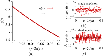
Figure 1: (Color online) (a) Pair-correlation function $g(r)$ close to contact for $N=512^{2}$ at density $\eta=0.698$ using LMC. Error bars are computed through $64$ independent simulations. $g(r)$ is fitted with a fourth-order polynomial. Difference between $g(r)$ and the polynomial fit with the single-precision data (b) and double-precision data (c) for the histogram.

To access the contact value of $g(r)$, we fit the histogram of pair distances obtained from LMC by a polynomial as shown in Fig. 1 and then extrapolate the fit to $r=2\sigma$ from the right. We choose the bin size as $\delta r=10^{-3}\sigma$. The histogram is limited to $r\in[2\sigma,2.1\sigma]$, and the fit is performed with a fourth-order polynomial. These parameters are sufficient to obtain a relative systematic error of less than $10^{-5}$. In the single-precision version of the algorithm, $g(r)$ shows correlated fluctuations which lead to systematic errors in the value of $g(r)$ for any single bin (see Fig. 1(b,c)). These errors are only due to floating point round-off of the pair-correlation function (the sampled configurations are essentially the same). However, they are periodic with zero mean and do not affect the fit significantly. We verified that single-precision rounding induces a relative systematic error smaller than $10^{-5}$ on the estimated value of $g(2\sigma^{+})$.

II.3.2 Dynamic pressure computation

In molecular dynamics, static configurations can be analyzed as before, but the pressure is computed directly and more efficiently from the collision rate via the virial theorem Erpenbeck_1977 ; Alder_1960 ; Hoover_1967 . This avoids binning and extrapolations. The non-dimensional virial pressure in two dimensions is given by

$$\beta P=\frac{N}{V}\left[1-\frac{\beta m}{2t_{\text{tot}}}\frac{1}{N}\sum_{\text{collisions}}b_{ij}\right]$$ (5)

where $t_{\text{tot}}$ is the total simulation time. The collision force $b_{ij}=\mathbf{r}_{ij}\cdot\mathbf{v}_{ij}$ is defined between the relative positions and relative velocities of the collision partners. In equilibrium, the average virial for hard disks equals Ladd_1987

$$\left\langle b_{ij}\right\rangle=-2\sigma\sqrt{\frac{\pi}{\beta m}}.$$ (6)

Therefore, the pressure is simply given by the collision rate $\Lambda=1/t_{0}$, the reciprocal of the mean free time $t_{0}$, as

$$\beta P=\frac{N}{V}\left[1+\frac{\sigma\sqrt{\pi\beta m}}{2}\Lambda\right].$$ (7)

To test the pressure computations, we compute the pressure with all algorithms at one representative state point. With each algorithm, we perform between 8 and 100 independent runs to compute the statistical standard error. Results obtained with the four algorithms agree within numerical accuracy to $\leq 10^{-4}$, which is sufficient for our purposes (see Table 1).

Algorithm	runs	disp./run	$\beta P(2\sigma)^{2}$	std. error
LMC	$64$	$6\times 10^{11}$	$9.17046$	$1.5\times 10^{-4}$
EDMD	$100$	$10^{10}$	$9.17076$	$1.8\times 10^{-4}$
ECMC	$32$	$5\times 10^{11}$	$9.17062$	$8.7\times 10^{-5}$
MPMC	$8$	$6\times 10^{13}$	$9.17078$	$4.5\times 10^{-5}$

Table 1: Test of the pressure computations for $N=256^{2}$ at $\eta=0.698$. The table lists for each algorithm the number of runs, number of displacements (disp.) per run, pressure, and standard error. Results of all four algorithms agree within their numerical accuracies.

III Performance comparison

One of the slowest processes during the time evolution of the hard-disk system at high density is the fluctuation of the global orientation order parameter

$$\Psi_{6}=\frac{1}{N}\sum_{j}\psi_{j},$$

which is the spatial average of the local orientational order parameter

$$\psi_{j}=\frac{1}{6}\sum_{k=1}^{6}\exp(i\,6\phi_{j,k}).$$ (8)

The sum is over the six closest neighbors $k$ of disk $j$, and $\phi_{j,k}$ is the angle between the shortest periodic vector equivalent to $\mathbf{x}_{k}-\mathbf{x}_{j}$ and a chosen fixed reference vector. This approach is simpler than using the Voronoi construction Bernard_2011 , without affecting the autocorrelation functions. To determine the efficiency of our algorithms, we track the autocorrelation function of $\Psi_{6}$ Bernard_2009 ,

$$C(\Delta t)=\frac{\left\langle\Psi_{6}(t)\Psi_{6}^{*}(t+\Delta t)\right\rangle_{t}}{\left\langle|\Psi_{6}|^{2}\right\rangle}.$$ (9)

The $\Psi_{6}\to\Psi_{6}+\pi$ symmetry in the square box imposes that $C(\Delta t)$ decays to zero for infinite times. In the asymptotic limit, the decay is exponential, $C(\Delta t)\propto\exp(-\Delta t/\tau)$, and we obtain the correlation time $\tau$ from a fit of the pure exponential part (see Fig. 2).

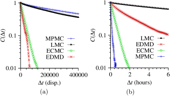
Figure 2: (Color online) Autocorrelation function of the global orientation order parameter $\Psi_{6}(t)$ for $N=512^{2}$, $\eta=0.698$ obtained with LMC, EDMD, ECMC, and MPMC. (a) Time is measured in number of attempted displacements (or collisions) per disk. (b) Time is measured in CPU or GPU hours.

We compare speeds for $N=512^{2}$ at $\eta=0.698$, that is, in the dense liquid close to the liquid–hexatic coexistence. Although still a liquid, the correlation length of the local orientational order parameter $\psi_{j}$ at this density is $\sim 50\sigma$. Such a large correlation length induces a long correlation time, and equilibration requires $>10^{6}$ trial moves per disk for LMC. For the test, each algorithm is set to its optimal internal parameters. Total simulation run times are on the order of $10^{3}\tau$ to $10^{4}\tau$.

Fig. 2 illustrates that the autocorrelation functions decay roughly as pure exponentials. The time unit in Fig. 2(a) corresponds to the number of attempted displacements per disk (number of collisions in the case of EDMD and ECMC). As expected, MPMC decays slightly more slowly than LMC because trial moves across cell boundaries are rejected. ECMC and EDMD are significantly faster than LMC, confirming that these two methods sample configuration space more efficiently, but slower than MPMC. The time unit in Fig. 2(b) corresponds to the real simulation time (CPU or GPU time).

Correlation times, number of attempted displacements per hour, and accelerations with respect to LMC are summarized in Table 2. EDMD and ECMC sample configuration space more efficiently by a factor of 39 times and 28 times, respectively, while MPMC samples configuration space slightly less efficiently by a factor of 0.9. Evidently, the efficiency of the simple LMC algorithm is improved significantly with speed-ups of $10$, $70$, and $320$ for EDMD, ECMC, and MPMC, respectively. Although speeds in Table 2 correspond to somewhat different hardware, as indicated in the methods section, the numbers give a clear idea of practical improvements that can be obtained with respect to LMC.

Algorithm	$\tau$/disp.	disp./hour	$\tau_{\text{LMC}}/\tau$	Speed-up
LMC	$7\times 10^{5}$	$6.5\times 10^{9}$	$1$	$1$
EDMD	$1.8\times 10^{4}$	$1.7\times 10^{9}$	$39$	$10$
ECMC	$2.5\times 10^{4}$	$1.6\times 10^{10}$	$28$	$70$
MPMC	$8\times 10^{5}$	$2.3\times 10^{12}$	$0.9$	$320$

Table 2: Speed comparison of the four hard-disk algorithms for $N=512^{2}$, $\eta=0.698$. The correlation time $\tau$ is measured in number of displacements (or collisions) per disk. disp./hour represents the number of displacements per hour achieved in our implementations. The two rightmost columns show the speed-up of the algorithms in number of displaced disks, and in terms of CPU or GPU time in comparison to LMC.

IV Results and discussion

IV.1 Equation of state at high density

In their seminal work, Alder and Wainwright observed a loop in the equation of state of hard disks Alder_1962 . As explained by Mayer and Wood Mayer_1965 (see also Furukawa_1982 ; Schrader_2009 ), this loop is a result of finite simulation sizes and therefore differs conceptually from a classic van der Waals loop, which is derived in the thermodynamic limit. The branches of the Mayer-Wood loop are thermodynamically stable, but vanish in the limit of infinite size.

It is known that the presence of a Mayer-Wood loop in the equation of state is observed in systems showing a first-order transition as well as systems showing a continuous transition Alonso_1999 . However, the behavior of these loops with increasing system size is different. For a first-order transition, the loop is present in the coexistence region and is caused by the interface free energy $\Delta F$. At a given density, the interface free energy per disk, $\Delta f=\Delta F/N$, can be computed by integrating the equation of state Bernard_2011 . In two dimensions, it scales as $\Delta f\propto N^{-1/2}$. In contrast, for a continuous transition, $\Delta f$ decays faster, normally such that $\Delta F$ is constant, that is $\Delta f\propto N^{-1}$, and the equation of state becomes monotonic for large enough systems. The scaling of $\Delta f$ with system size, together with a fixed finite separation of the peaks for large system sizes, is a reliable indicator of the first-order character of a phase transition Lee_1991 .

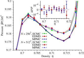
Figure 3: (Color online) Equation of state from ECMC, EDMD, and MPMC for $N=256^{2}$ and $N=512^{2}$. Error bars are mostly smaller than the symbols. Results agree within one standard deviation. The inset shows the relative pressure difference $\Delta P/P$ of EDMD and MPMC with respect to ECMC for $N=256^{2}$.

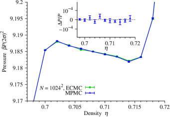
Figure 4: (Color online) Equation of state from ECMC and MPMC for $N=1024^{2}$. Error bars are mostly smaller than the symbols. Results agree within one standard deviation. The inset shows the relative pressure difference $\Delta P/P$ of MPMC with respect to ECMC.

Fig. 3 shows the equation of state for $N=256^{2}$ and $N=512^{2}$, obtained with ECMC, EDMD, and MDMC. Error bars (standard errors) are computed through independent simulations. The inset shows the relative pressure difference $\Delta P/P$ of EDMD and MDMC with ECMC. Error bars correspond again to the standard error on $\Delta P/P$. We observe that the three independent simulations agree. In a similar way, Fig. 4 compares results from ECMC and MPMC for $N=1024^{2}$. For this system size and the currently available computer hardware, equilibration with EDMD takes too long to be practical. Again, all results agree within standard deviations. Note that while the Mayer-Wood loop shrinks with system size, the position of the local extrema stay fixed close to $\eta=0.702$ and $\eta=0.714$.

IV.2 Orientational order parameter field

The degree and distribution of local order in a system can be analyzed with the help of order parameters. By averaging a given order parameter attached to each particle over a small sampling area surrounding the particle, we obtain a continuous function, the corresponding order parameter field. Typical sampling areas used in this work contain between 5 and 20 disks.

To show the separation of the liquid and the hexatic phase, we graphically represent the orientational order parameter field $\psi(\mathbf{x})$ for configurations at densities where coexistence occurs. As for any first-order phase transition in two dimensions, the characteristic geometry of the region of the minority phase with increasing density is expected to change from an approximately circular bubble into a parallel stripe and again into a circular bubble. Ref. Bernard_2011 used the projection of the local orientational order $\psi_{k}$ on the global orientational order $\Psi_{6}$ and a linear color code. This projection is not a unique measure for the orientational order parameter field. Instead, in Fig. 5, we use a circular color code on data obtained by long MPMC simulations with $N=1024^{2}$.

We observe that the system is uniformly liquid at $\eta=0.700$ and the color fluctuates on the scale of the correlation length. At $\eta=0.704$, the representations indicate the presence of a circular bubble of hexatic phase, visible as a large region of constant purple color, whereas at $\eta=0.708$ a stripe minimizes the interfacial free energy. The hexatic phase is now visible in blue, while the liquid is characterized by fluctuations of the direction of $\Psi_{6}$. The constant color in the region of the hexatic phase confirms the presence of the same orientational order across the system. Additional important evidence for the nature of the transition is provided by the spatial correspondence between variations in local density and orientational order, which are included as a movie in the supplemental material of this work. The movie illustrates for the density $\eta=0.71$ that the system is ergodic by seeing the patches of the two phases appear and disappear at different locations but with roughly fixed ratio of areas.

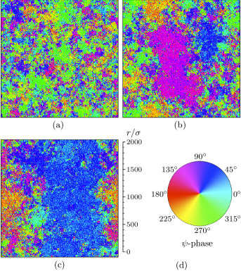
Figure 5: (Color online) Orientational order parameter field $\psi(\mathbf{x})$ of configurations obtained with the MPMC algorithm for system size $N=1024^{2}$. With increasing density, (a) pure liquid ($\eta=0.700$), (b) a bubble of hexatic phase ($\eta=0.704$), and (c) a stripe regime of hexatic phase ($\eta=0.708$) are visible. The interface between the liquid and the hexatic phase is extremely rough. (d) A scale bar illustrates the size of the fluctuations. The phase of $\psi$ is represented via the color wheel.

IV.3 Positional order parameter field

To identify the structure of the ordered phase in coexistence with the liquid, we analyze the positional order in the system. The goal is to distinguish the hexatic phase, which has short-range positional order (characterized by exponential decay of the correlation function) and quasi-long-range orientational order (algebraic decay), from the two-dimensional solid, which has quasi-long range positional order Mermin_1968 and long-range orientational order (no complete decay).

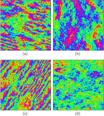
Figure 6: (Color online) Positional order parameter field $\chi(\mathbf{x})$ of configurations obtained with (a,b) the MPMC and (c,d) ECMC algorithms for system size $N=1024^{2}$. (a,c) In the hexatic phase ($\eta=0.718$), positional order is short-range. (b,d) Towards higher density ($\eta=0.720$), fluctuations are much weaker and bounded, as expected for a continuous transition to a solid phase. The scale bar and the color code for the $\chi$-phase are identical to the scale bar and the color code in Fig. 5.

In Bernard_2011 , the positional order was analyzed using the two-dimensional pair-correlation function in direct space and the decay of the positional correlation function at the wave vector $\mathbf{q}_{0}$ corresponding to the maximum value of the first diffraction peak of the structure factor

$$S(\mathbf{q})=\frac{1}{N}\sum_{n,m}\exp(i\mathbf{q}\cdot(\mathbf{x}_{n}-\mathbf{x}_{m})).$$ (10)

With this classic method, the wave vector $\mathbf{q}_{0}$ must be chosen carefully to correspond to a diffraction peak. In some previous works Mak_2006 ; Bagchi_1996 , it was assumed that $\mathbf{q}_{0}$ would correspond to the reciprocal vector of a perfect triangular lattice of edge length $a_{0}$, namely $|\mathbf{q}_{0}|=2\pi/(a_{0}\sqrt{3}/2)$. This assumption is not correct because the solid phase has a finite density of vacancies and other defects in equilibrium, which increases the effective lattice constant Bernard_2011 .

We visualize the positional order parameter field $\chi(\mathbf{x})$ calculated from the positional order parameter

$$\chi_{j}=\exp(i\mathbf{q}_{0}\cdot\mathbf{x}_{j}).$$ (11)

slightly above the upper critical density of coexistence with the liquid (Fig. 6). At $\eta=0.718$, the system resembles a patchwork of independent, solid-like regions of size in the order of a few hundred $\sigma$. Some regions show almost constant $\chi$, while others are characterized by regular interference fringes (oscillatory waves) with a fixed wave vector. It can be shown that each end of a fringe corresponds to one unpaired dislocation . We find that fringes can be made to disappear separately in each region by small rotations of $\mathbf{q}_{0}$ around the origin. This behavior is consistent with the existence of small-angle grain boundaries separating neighboring solid-like regions, exactly as predicted by the KTHNY scenario Fisher_1979 . Note that if fringes disappear on one side of a boundary separating two regions, they necessarily have to reappear on the other side with the sequence of the colors reversed.

On physical grounds, the hexatic phase is not expected to be stable up to close packing. Indeed, already at $\eta=0.720$, the positional order field shown in Fig. 6 fluctuates much more slowly and is highly correlated throughout the system as expected for a solid phase.

IV.4 Positional correlation function

The decay of positional order can be analyzed using the positional correlation function in reciprocal space,

$$C_{\mathbf{q}_{0}}(r)=\left\langle\exp(i\mathbf{q}_{0}\cdot(\mathbf{x}_{n}-\mathbf{x}_{m}))\right\rangle.$$ (12)

The averaging for $C_{\mathbf{q}_{0}}(r)$ is done on two levels. First, we average over neighboring pairs that satisfy $|\mathbf{x}_{n}-\mathbf{x}_{m}|\in[r-\sigma,r+\sigma]$. In addition, we conduct an average over independent configurations, which can be a time average or an ensemble average. For details on the configuration averaging see Appendix A. As the system can perform global rotations during the simulations, $\mathbf{q}_{0}$ rotates from one configuration to the other. Each configuration is individually rotated so that $\Psi_{6}$ is aligned in the same direction for all of them. We verified that alignment errors are sufficiently small and can be neglected. As a result of the configuration average, finite-size effects present at large distances $r$ in the form of interferences are suppressed.

Fig. 7 shows $C_{\mathbf{q}_{0}}(r)$ at $\eta=0.718$ and $\eta=0.720$. The results of ECMC and MPMC are again in good agreement. We observe that $C_{\mathbf{q}_{0}}(r)$ decays exponentially at $\eta=0.718$. Therefore, $\eta=0.718$ cannot be in the solid phase. The length scale of the exponential decay is in the order of $100\sigma$, which corresponds approximately to the width of the interference fringes in Fig. 6. Since the coexistence phase ends at $\eta\simeq 0.716$, the region $\eta\gtrsim 0.716$ is thus hexatic. We have shown once more that the first-order transition observed in Fig. 3 connects a liquid and a hexatic phase.

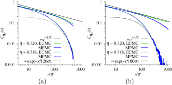
Figure 7: (Color online) The positional correlation function $C_{\mathbf{q}_{0}}(r)$ shows exponential decay at density $\eta=0.718$ and approaches a power law $\propto r^{-1/3}$ at $\eta=0.720$. (a) System size $N=512^{2}$: Excellent agreement between ECMC and MPMC. (b) System size $N=1024^{2}$: Excellent agreement in the hexatic phase ($\eta=0.718$) and fair agreement at the approach of the solid phase ($\eta=0.720$). Our algorithms fall out of strict equilibrium in the solid and long-scale correlations become sensitive to the boundary conditions.

The positional order increases drastically at $\eta=0.720$. $C_{\mathbf{q}_{0}}(r)$ decays almost as a power law, $r^{-1/3}$, which is the stability limit for the solid phase in the KTHNY theory. Thus, the stability regime of the hexatic phase comprises a narrow range of density. An additional characterization of the hexatic phase with ECMC including a study of the diffraction peak shape can be found in Bernard_2011b and in the supplemental material of Bernard_2011 . The continuous transformation to the solid phase and the nature of the hexatic phase agree with the KTHNY scenario.

Slight variations in the positional correlations can be observed in Fig. 7 at density $\eta=0.720$ for distances comparable to the system size. Two factors play a role. First, the relaxation becomes very slow at the onset of the solid phase. Our largest system no longer achieves full global rotations with respect to $\Psi_{6}$. Second, the positional correlations span the whole simulation box and therefore depend slightly on the orientation of the crystal. Longer and larger simulations are necessary to determine the location of the hexatic–solid transition with good precision. However, the general absence of a loop in pressure is sufficient to rule out a first-order transition. We note that while our simulations fall out of strict equilibrium with respect to global rotations in the solid phase, they remain fully ergodic within our simulation times on both sides of the liquid–hexatic transition.

V Conclusion

We analyzed the thermodynamic behavior of the hard-disk system close to the melting transition using independent implementations of three different simulation algorithms to sample configuration space and two distinct approaches for the pressure computation. The equation of state data of Ref. Bernard_2011 are confirmed within numerical accuracy both qualitatively and quantitatively. Typical relative errors are $\lesssim 10^{-4}$, more than one order of magnitude smaller than finite-size effects for systems with up to $N=1024^{2}$ particles. Such finite-size effects are manifested in the form of a Mayer-Wood loop in the equation of state. Our analysis of orientational and positional order parameters confirms the presence of a first-order phase transition from liquid order to hexatic order and a continuous phase transition from hexatic order to a solid phase.

Appendix A Role of configuration averaging

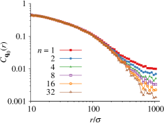
Figure 8: (Color online) Influence of the configuration averaging on the positional configuration functions in the hexatic phase. For single configurations ($n=1$, data incoherently averaged), positional correlations cannot decay below a level given by the square root of the ratio of the correlated domain size to the system size. Coherent averaging over $n=2$, $4$, $8$, $16$, and $32$ configurations reduces the noise level and the correlations. The data corresponds to a single long MPMC run with $N=1024^{2}$ particles at density $\eta=0.718$.

It is instructive to analyze the influence of configuration averaging that we employ to calculate the correlation function $C_{\mathbf{q}_{0}}(r)$. We define a configuration average as the time average or the ensemble average of $C_{\mathbf{q}_{0}}(r)$ over individual configurations. This coherent averaging procedure stands in contrast to the incoherent averaging procedure, where we bin the function $C_{\mathbf{q}_{0}}(r)$, determine the maximum within each of the bins, and average the maxima. As shown in Fig. 8, for incoherently averaged single configurations the long-distance correlations do not decay below a sampling threshold that is set by the inverse square root of the number of independent domains in the sample. For our large system of $N=1024^{2}$ particles, given that the sample size is $L/2\sim 1000\sigma$ and the positional correlation length is in the order of $100\sigma$, there are about 100 independent domains. Residual correlations visible in the figure as a plateau at large values of $r/\sigma$ correspond to what would be expected from about $100$ independent randomly positioned (yet equally oriented) lattices. As illustrated in the figure, coherent averaging over oriented configurations increases the effective number of independent domains, thus to reduce the noise level. The same effect would be obtained if we could equilibrate yet larger systems.

- (1) N. Metropolis, A. W. Rosenbluth, M. N. Rosenbluth, A. H. Teller, E. Teller, J. Chem. Phys. 21 1087 (1953).
- (2) B. J. Alder, T. E. Wainwright, J. Chem. Phys. 27, 1208 (1957).
- (3) B. J. Alder, T. E. Wainwright, Phys. Rev. 127, 359 (1962).
- (4) K. J. Strandburg, Rev. Mod. Phys. 60, 161 (1988).
- (5) J. G. Dash, Rev. Mod. Phys. 71, 1737 (1999).
- (6) E. P. Bernard, W. Krauth, D. B. Wilson, Phys. Rev. E 80, 056704 (2009).
- (7) E. P. Bernard, W. Krauth, Phys. Rev. Lett. 107, 155704 (2011).
- (8) J. M. Kosterlitz, D. J. Thouless, J. Phys. C 5, L124 (1972).
- (9) B. I. Halperin, D. R. Nelson, Phys. Rev. Lett. 41, 121 (1978).
- (10) D. R. Nelson, B. I. Halperin, Phys. Rev. B 19, 2457 (1979).
- (11) A. P. Young, Phys. Rev. B 19, 1855 (1979).
- (12) A. Jaster, Phys. Rev. E 59, 2594 (1999).
- (13) C. H. Mak, Phys. Rev. E 73, 065104 (2006).
- (14) D. S. Fisher, B. I. Halperin, R. Morf, Phys. Rev. B 20, 4692 (1979).
- (15) S. T. Chui, Phys. Rev. B 28, 178 (1983).
- (16) H. Kleinert, Phys. Lett. A 95, 381 (1983).
- (17) T. V. Ramakrishnan, Phys. Rev. Lett. 48, 541 (1982).
- (18) H. Weber, D. Marx, K. Binder, Phys. Rev. B 51, 14636 (1995).
- (19) J. A. Zollweg, G. V. Chester, Phys. Rev. B 46, 11186 (1992).
- (20) J. Lee, K. J. Strandburg, Phys. Rev. B 46, 11190 (1992).
- (21) J. E. Mayer, W. W. Wood, J. Chem. Phys. 42, 4268 (1965).
- (22) H. Furukawa, K. Binder, Phys. Rev. A 26, 556 (1982).
- (23) M. Schrader, P. Virnau, K. Binder, Phys. Rev. E 79, 061104 (2009).
- (24) J. A. Anderson, E. Jankowski, T. L. Grubb, M. Engel, S. C. Glotzer submitted.
- (25) M. Isobe, Int. J. Mod. Phys. C 10, 1281 (1999).
- (26) W. Krauth, Statistical Mechanics: Algorithms and Computations, Oxford University Press (2006).
- (27) A. Uhlherr, S. J. Leak, N. E. Adam, P. E. Nyberg, M. Doxastakis, V. G. Mavrantzas, D. N. Theodorou, Comp. Phys. Commun. 144, 1 (2002).
- (28) G. Pawley, K. Bowler, R. Kenway, D. Wallace, Comp. Phys. Commun. 37, 251 (1985).
- (29) D. C. Rapaport, J. Comp. Phys. 34, 184 (1980).
- (30) B. D. Lubachevsky, J. Comp. Phys. 94, 255 (1991).
- (31) M. Marin, D. Risso, P. Cordero, J. Comp. Phys. 109, 306 (1993).
- (32) M. Marin, P. Cordero, Comp. Phys. Commun. 92, 214 (1995).
- (33) J. J. Erpenbeck, W. W. Wood, in Modern Theoretical Chemistry Vol.6, Statistical Mechanics Part B, edited by B. J. Berne (Plenum, New York, 1977).
- (34) B. J. Alder, T. E. Wainwright, J. Chem. Phys. 33, 1439 (1960).
- (35) W. G Hoover, B. J. Alder, J. Chem. Phys. 46, 686 (1967).
- (36) A. C. J. Ladd, W. E. Alley, B. J. Alder, J. Stat. Phys. 48, 1147 (1987).
- (37) J. J. Alonso, J. F. Fernández, Phys. Rev. E 59, 2659 (1999).
- (38) J. Lee, J. M. Kosterlitz, Phys. Rev. B 43, 3265 (1991).
- (39) N. D. Mermin, Phys. Rev. 176, 250 (1968).
- (40) K. Bagchi, H. C. Andersen, W. Swope, Phys. Rev. Lett. 76, 255 (1996).
- (41) A. Howie, M. J. Whelan, Proc. Roy. Soc. London A: Math. Phys. Sci. 267, 206 (1962).
- (42) E. P. Bernard, Doctoral Thesis, University Pierre et Marie Curie, Paris (2011). http://tel.archives-ouvertes.fr/tel-00637330/en