Heat equation approach to geometric changes of the torus Laughlin-state

Abstract

We study the second quantized -or guiding center- description of the torus Laughlin state. Our main focus is the change of the guiding center degrees of freedom with the torus geometry, which we show to be generated by a two-body operator. We demonstrate that this operator can be used to evolve the full torus Laughlin state at given modular parameter $\tau$ from its simple (Slater-determinant) thin torus limit, thus giving rise to a new presentation of the torus Laughlin state in terms of its “root partition” and an exponential of a two-body operator. This operator therefore generates in particular the adiabatic evolution between Laughlin states on regular tori and the quasi-one-dimensional thin torus limit. We make contact with the recently introduced notion of a “Hall viscosity” for fractional quantum Hall states, to which our two-body operator is naturally related, and which serves as a demonstration of our method to generate the Laughlin state on the torus.

I Introduction

The discovery of the fractional quantum Hall effectTsui et al. (1982) has led to a series of remarkable theoretical developments. Much insight has flowed from principles that govern the construction of certain “special wave functions”Laughlin (1983); Moore and Read (1991); Read and Rezayi (1999); Haldane and Rezayi (1988); Halperin (1983); Simon et al. (2007) and their relation with conformal field theory (CFT)Moore and Read (1991), and/or their interpretation in a composite fermion pictureJain (1989). The credibility of this approach is greatly enhanced by the construction of parent Hamiltonians for such wave functions, which has been possible in many interesting cases.Read and Rezayi (1999); Haldane and Rezayi (1988); Haldane (1983); Trugman and Kivelson (1985); Greiter et al. (1991) This very particular class of quasi-solvable Hamiltonians consists of Landau level projected ultra-local interactions, which enforce the analytic properties that uniquely characterize the respective ground state. The prime example for such a parent Hamiltonian is given by the $V_{1}$-pseudopotential,Haldane (1983) which is a pairwise (two-particle) projection operator onto states of relative angular momentum $1$ within the lowest Landau level (LLL). Its unique ground state at filling factor $\nu=1/3$ is the Laughlin state corresponding to this filling.

Due to the Landau level projection, the pseudo-potential Hamiltonian acts only on the “guiding center” degrees of freedom, which exhaust the large degeneracy within a given Landau level, and commute with the generators of inter-level transitions. (The latter are related to the kinetic momenta of the particles, see below. For a review of physics in a magnetic field, the reader is referred to Ref. MacDonald, 1994.) It is therefore beneficial to make the action of the Hamiltonian on guiding center variables manifest. This is in particular the case when the Hamiltonian is expressed using creation/annihilation operators for a set of eigenstates, say, of one of the two non-commuting guiding center components, which form a basis for the LLL. In numerics, such a second quantized “guiding center” description of the Hamiltonian is essential to make use of the reduced Hilbert space dimensionality owing to the LLL projection. We illustrate this procedure for the cylinder geometry, for reasons that will soon become apparent. To this end, we introduce a set of LLL basis states as described above, given by:

$$\phi_{n}(z)=\xi^{n}e^{-\frac{1}{2}x^{2}}e^{-\frac{1}{2}n^{2}/r^{2}}\,$$ (1)

where $\xi=e^{z/r}$ is an analytic function of $z=x+iy$ that satisfies periodic boundary conditions in $y$, appropriate for a cylinder of perimeter $2\pi r$ (using Landau gauge, ${\bf A}=(0,x)$). These orbitals are eigenstates of the x-component of the guiding center with eigenvalues $n/r$, where, for the time being, we set the magnetic length $l_{B}$ equal to $1$. The 1/3-Laughlin state on the cylinder is then expressed asRezayi and Haldane (1994)

$$\psi_{1/3}(z_{1}\dotsc z_{N})=\prod_{i<j}(\xi_{i}-\xi_{j})^{3}\times e^{-\frac{1}{2}\sum_{k}x_{k}^{2}}\,.$$ (2)

With respect to the basis Eq. (1), the $V_{1}$ pseudo-potential takes on the following second quantized form (cf, e.g., Ref. Lee and Leinaas, 2004):

$$\begin{split}\hat{V}_{1}&=\sum_{R}Q^{\dagger}_{R}Q_{R}\\ Q_{R}&=\sum_{x}x\exp(-x^{2}/r^{2})\,c_{R-x}c_{R+x}\end{split}$$ (3)

In the first line, the sum goes over both integer and half-odd integer values of $R$, whereas in the second it goes over integer (half-odd integer) if $R$ is integer (half-odd integer), such that labels $R\pm x$ are then always integer.

The one parameter family of models (3) share many features with one-dimensional (1D) lattice models that arise elsewhere in solid state physics, such as translational invariance and short ranged (exponentially decaying) interactions. It is thus not surprising that it has recently been proposed to be of use in the absence of (proper) Landau level physics, e.g., in flat band solids both withQi (2011) and withoutWang and Scarola (2011) non-zero Chern numbers, and in quite general terms in Ref. Seidel et al., 2005.

Despite the usefulness of the second quantized description (3) of the pseudo-potential, it would be very difficult to solve for the zero energy eigenstates of the model in this form, or to even know analytically that such zero energy eigenstates exist. For this we rely on the original first-quantized definition of the pseudo-potential $\hat{V}_{1}$, and on the explicitly known analytic form of the Laughlin state, Eq. (2), in terms of ordinary position variables. It would be highly non-trivial, however, to come up with such a first quantized language for the problem Eq. (3) if its connection to LLL orbitals were not a priori known. This is so because this language becomes available only after proper embedding of the degrees of freedom associated with the operators $c_{n}$, $c_{n}^{\dagger}$ in Eq. (3) into a larger Hilbert space. In Eq. (3), no information is retained about the kinetic momenta that determine the structure of the Landau levels. Indeed, as Haldane has recently shown,Haldane (2011) by making these kinetic momenta subject to a different metric from that entering the interactions, one obtains a different way to naturally embed the problem (3) into the larger Hilbert space of square integrable functions. In this setup, Eq. (3) remains unaltered, but the resulting wave function loses the analytic properties of Eq. (2) that make the problem tractable.Haldane (2011); Qiu et al. (2012) Moreover, the solid state applications mentioned initially represent yet another way to embed the problem (3) into a larger Hilbert space.

These considerations show that “interaction only” models such as (3), especially ones that share the “center-of-mass conserving” property,Seidel et al. (2005) may enjoy a considerable range of applications, but at the same time, may be quite hard to solve in general. This is chiefly due to the fact that the Laughlin state, in its second quantized/guiding center presentation, is quite a bit more complicated than in its analytic first quantized form Eq. (2). While no closed form seems to be known for the amplitudes $\langle 0|c_{n_{1}}\dotsc c_{n_{N}}|\psi_{1/3}\rangle$, much progress has recently been made in understanding their structure for the cylinder geometry, and for any other geometry in which the analytic part of Laughlin’s wave function is given by a polynomial. Indeed, for Laughlin states and many other quantum Hall trial wave functions, these polynomials have been identified as Jack polynomials, multiplied by Jastrow factors.Bernevig and Haldane (2008a, b) This allows the amplitudes $\langle 0|c_{n_{1}}\dotsc c_{n_{N}}|\psi_{1/3}\rangle$ to be determined recursively. For the cylinder Laughlin state, this can be sketched as follows. We consider the expansion of Eq. (2) into monomials,

$$\begin{split}\psi_{1/3}(z_{1}\dotsc z_{N})=\sum_{\{n_{k}\}}C_{\{n_{k}\}}\prod_{k}\xi_{k}^{n_{k}}e^{-\frac{1}{2}x_{k}^{2}}\end{split}$$ (4)

The product in the above equation can be interpreted as a state with definite single particle occupation numbers, up to a normalization. (The $C_{\{n_{k}\}}$ have the proper (anti)-symmetry to allow (anti)-symmetrization of the product.) This normalization is readily read from Eq. (1). We thus haveRezayi and Haldane (1994)

$$|\psi_{1/3}\rangle_{r}=\sum_{\{n_{k}\}}e^{\frac{1}{2r^{2}}\sum_{k}n_{k}^{2}}C_{\{n_{k}\}}\;c^{\dagger}_{n_{N}}\dotsc c^{\dagger}_{n_{1}}|0\rangle\,.$$ (5)

The monomial coefficients do not depend on $r$, and are known recursively, starting from the coefficient of the “root configuration” $c^{\dagger}_{n_{N}}\dotsc c^{\dagger}_{n_{1}}|0\rangle=|10010010010\dotsc\rangle$ through a process known as “inward squeezing”.Bernevig and Haldane (2008a, b)

A remarkable aspect of Eq. (5) is that the dependence on geometry, in this case the cylinder radius $r$, comes in only through the trivial normalization factor. This is matched by a similarly trivial $r$-dependence of the interaction $\hat{V}_{1}$. It is quite easy to see that the condition that the Hamiltonian Eq. (3) has a zero energy eigenstate (which, by positive semi-definiteness, must be a ground state), which reduces to $Q_{R}|\psi_{1/3}\rangle_{r}=0$ $\forall R$, yields an $r$-independent condition on the coefficients $C_{\{n_{k}\}}$. In this way it becomes manifest that regardless of the value or $r$, one is always solving the same problem, which is intuitively clear from the simple analytic form of the Laughlin wave function (2) and its trivial $r$-dependence. It should also be emphasized that the simple $r$-dependence of Eq. (5) is not particular to the Laughlin state. It is a direct consequence of the polynomial form of the wave function, and carries over without change to any quantum Hall trial state on the cylinder.

The situation is rather different for the torus geometry. The main purpose of this work will be to get a handle on the guiding center presentation of the torus Laughlin states. In the remainder of this introduction, we review some well known facts that make life more complicated on the torus.

In first quantized language, we pass to the torus by introducing periodic boundary conditions in the complex plane along two fundamental periods $L_{1}$ and $L_{2}$, where $L_{1}$ is taken to be real, and $\mbox{Im}L_{2}>0$ (Fig. 1). The geometry of the torus can be parameterized by $\tau=L_{2}/L_{1}$, the modular parameter. The Laughlin state at general filling factor $1/q$ then becomesHaldane and Rezayi (1985)

$$\psi_{1/q}^{\ell}(z_{1}\dotsc z_{N})=\exp(-\frac{1}{2}\sum_{k}y_{k}^{2})\,F^{\ell}(Z,\tau)\prod_{i<j}\theta_{1}(\frac{z_{i}-z_{j}}{L_{1}},\tau)^{q}\,$$ (6)

Here, $\theta_{1}(z,\tau)$ is the odd Jacobi theta-function, and for the factor depending on the “center of mass” $Z=z_{1}+\dotsc z_{N}$, which also depends on an additional label $\ell=0\dotsc q-1$ corresponding to a choice of basis in the $q$-fold degenerateWen and Niu (1990) ground state space, we adopt the convention of Ref. Read and Rezayi, 1996:

$$F^{\ell}(Z,\tau)=\theta\left[\begin{array}[]{c}\frac{\ell}{q}+\frac{L-q}{2q}\\ -\frac{L-q}{2}\end{array}\right](qZ/L_{1},q\tau)\,.$$ (7)

Here, $\theta{a\brack b}(z,\tau)$ is the Jacobi theta function of characteristics $a$ and $b$, and $L=L_{1}\mbox{Im}L_{2}/(2\pi)$ is the number of flux quanta penetrating the surface of the torus.

Thus, while the Laughlin state is still of the general form of a Gaussian factor multiplying an analytic function in the complex particle coordinates $z_{i}$, the latter is not of polynomial form. As a result, to the best of our knowledge, there is currently no detailed understanding of the structure of the guiding center description of this state. By this we mean a general understanding of the coefficients of the analog of Eq. (5):

$$|\psi_{1/3}^{\ell}\rangle_{\tau}=\sum_{\{n_{k}\}}C_{\{n_{k}\}}^{\ell}(\tau)\;c^{\dagger}_{n_{N}}\dotsc c^{\dagger}_{n_{1}}|0\rangle\,.$$ (8)

In particular, the $\tau$-dependence of the coefficients $C^{\ell}_{\{n_{k}\}}(\tau)$ is not of a simple form reminiscent of the $r$-dependence explicit in Eq. (5). Moreover, intuitively, one would still expect that these coefficients can be generated from the dominance pattern, i.e., $100100100\dotsc$ at $\nu=1/3$. Indeed, this configuration is still dominant on the torus, in the sense that it is the configuration that dominates in the thin torus limitSeidel et al. (2005); Bergholtz and Karlhede (2005); Seidel and Lee (2006); Bergholtz and Karlhede (2006). The success of the thin torus approach in determining physical properties, such as Abelian and non-Abelian statisticsSeidel and Lee (2007); Seidel (2008); Flavin and Seidel (2011); Flavin et al. (2012) and the presence of gapless excitationsSeidel and Yang (2011), suggests that even on the torus these patterns allow for a reconstruction of the full many-body wave function. On the other hand, there is no notion of “inward” squeezing on the torus, due to periodic boundary conditions. The main result of this paper will be the development of a machinery for the above mentioned reconstruction of the full torus Laughlin state in the guiding center description, from the thin torus state. Since as an additional complication, such machinery can be expected to depend non-trivially on $\tau$, we first focus our attention on the dependence of the coefficients $C^{\ell}_{\{n_{k}\}}(\tau)$ on the geometric parameter.

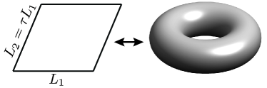
Figure 1: Fundamental domain for torus wave functions.

As a final remark, we point outHaldane and Rezayi (1985) that the torus Laughlin states at $\nu=1/3$ are still the unique ground state of the $V_{1}$ pseudo-potential. Its second quantized form agrees with a straightforward periodization of the model (3), with

$$Q_{R}=\sum_{0<x<L/2\atop x+R\in\mathbb{Z}}\;\sum_{m\in\mathbb{Z}}(x+mL)\exp[\frac{2\pi i\tau}{L}(x+mL)^{2}]\,c_{R-x}c_{R+x}\,.$$ (9)

One sees that for $\tau=i|L_{2}|/2\pi r$, $L_{2}=iL/r$, this reduces to the cylinder form Eq. (3) for $L\rightarrow\infty$, and respects the periodic boundary condition $c_{n}=c_{n+L}$ otherwise. (Eq. (9) is valid for general complex $\tau$, though). One therefore passes from Eq. (3) to Eq. (9) (with imaginary $\tau$) through straightforward introduction of periodic boundary conditions (PBCs). Yet the solution of Eq. (9) is arguably much less under control. The introduction of PBCs is a standard and very useful tool throughout solid state physics. We thus expect that a better understanding of the guiding center description of the torus Laughlin state will also benefit the solid state applicationsWang and Scarola (2011); Qi (2011) mentioned initially.

The remainder of the paper is organized as follows. In section II we construct a two-body operators that generated the changes in the guiding center variables of the torus Laughlin state with modular parameter $\tau$. Sections II.1 and II.2 highlight further formal similarities and differences between the cylinder and the torus. Sec. II.3 presents the heat equation for the $\tau$-derivative of the analytic Laughlin state. Sec. II.4 introduces a 2D to 1D mapping, which is our device for embedding lowest Landau levels at different modular parameter $\tau$ into the same larger Hilbert space. In Sec. II.5 we derive the generator mentioned above. In Sec. II.6 we symmetrize this operator and present a byproduct of this study, a hitherto unknown class of two-body operators that annihilate the torus Laughlin state. In Sec. II.7 we postulate a presentation of the torus Laughlin state in terms of its thin torus, or “dominance” pattern, and the class of two-body operators generating changes in geometry. In Sec. III we demonstrate the postulate of Sec. II.7 numerically, and work out the relation of our generator with the Hall viscosityRead (2009), which we calculate numerically as a demonstration of analytical results, comparing the resulting data to earlier numerical studies. We discuss our results in Sec. IV, and conclude in Sec. V. A small Appendix discusses a minor technical detail.

II Construction of the 2-body operator

II.1 A final look at the cylinder case

As motivated above, to establish a machinery that generates the full guiding center description of the Laughlin state from the root configuration, a natural starting point is to get under control how this description changes with the geometric parameter $\tau$. To this end, we will seek to construct an operator that generates changes of the guiding center degrees of freedom to first order in $d\tau$. The similar problem for the cylinder, where $r$ is the geometric parameter, is comparatively trivial and was already addressed in the introduction. For later reference, it is instructive to first cast these results in terms of a generator of infinitesimal changes in the parameter $r^{-2}$. Eq. (5) can be written as

$$|\psi_{1/3}\rangle_{r^{\prime}}=e^{(r^{\prime-2}-r^{-2})G_{r^{-2}}}|\psi_{1/3}\rangle_{r}$$ (10)

where

$$G_{r^{-2}}=\frac{1}{2}\sum_{n}n^{2}c^{\dagger}_{n}c_{n}$$ (11)

is the generator of changes in the geometric parameter $r^{-2}$. Note that it is independent of $r$. We emphasize again that (10), (11) are very general, and apply to other quantum Hall trial states on the cylinder as well. In writing (10), we leave it understood that the exponentiated operator generates the change of the guiding center degrees of freedom only; it does not generate in any way the change of the LLL orbitals themselves as a function of $r$, Eq. (1). We are only concerned here with the change in guiding center degrees of freedom, since the object of study is the second quantized Hamiltonian Eq. (3), in which degrees of freedom associated with kinetic momenta are not retained. We will thus carefully distinguish from now on between the Laughlin wave function $\psi_{1/3}\equiv\psi_{1/3}(z_{1}\dotsc z_{N};r)$, which lives in the full Hilbert space of square integrable functions over some domain, and the ket $|\psi_{1/3}\rangle_{r}$, which lives in an abstract Hilbert space denoted $\cal L$ that is isomorphic to the LLL for any given value of cylinder radius $r$. Similar conventions will be used below for the torus. In $\cal L$, therefore, all those orbitals with the same guiding center quantum number $n$ become identified, which originally belonged to different LLLs corresponding to different values of the parameter $r$.

We note that a similarly universal operator that generates changes of the guiding center degrees of freedom in response to a change in geometry can be obtained on the plane.Read and Rezayi (2011); Qiu et al. (2012) Here, since a geometric deformation by means of uniform strain does not affect boundary conditions, such a deformation is implemented by a change in the metric, and unlike in Eq. (10), the operation implementing this deformation is unitary.

On the other hand, it is worth pointing out that in (10), the lack of unitarity leads to a breakdown of the equation in the “thin cylinder” limit $r\rightarrow 0$, in which $|\psi_{1/3}\rangle_{r}$ approaches $|100100100\dotsc\rangle$. The equation remains valid for arbitrarily small but finite $r$, where the limiting state $|100100100\dotsc\rangle$ receives arbitrarily small corrections, which are, however, important and may not be dropped, since they become large under the non-unitary evolution facilitated by the exponential operator. This is immediately clear from the fact that the thin cylinder state is an eigenstate of the one-body operator in the exponent. This operator is thus not capable of generating the off-diagonal matrix element needed to “squeeze” the full many-body wave function out of the thin cylinder state, i.e., the root configuration. Eq. (10) is thus not a tool to generate the full cylinder Laughlin state out of the root configuration. For the cylinder, however, other such tools are already available, as mentioned in the Introduction.Bernevig and Haldane (2008a, b)

II.2 General considerations for the generator on the torus

We desire to construct an operator analogous to $G_{r^{-2}}$ for the torus Laughlin state, which generates changes in the guiding center variables of the state in $\tau$. This operator is thus defined by the following equation:

$$\nabla_{\tau}|\psi_{1/q}^{\ell}(\tau)\rangle={{\bf G}}_{\tau}|\psi_{1/q}^{\ell}(\tau)\rangle\,.$$ (12)

Here, ${{\bf G}}_{\tau}$ denotes the operator valued two-component object $(G_{\tau_{x}},G_{\tau_{y}})$, and $\nabla_{\tau}\equiv(\partial_{\tau_{x}},\partial_{\tau_{y}})$. Note that we require that ${{\bf G}}_{\tau}$ is independent of the label $\ell$ distinguishing the $q$ degenerate Laughlin states $|\psi_{1/q}^{\ell}(\tau)\rangle$, at given filling factor $1/q$ and given $\tau$.

To highlight considerable differences with the similar problem on the cylinder, we now show that it follows easily from these assumptions that, unlike for the cylinder, the components of ${{\bf G}}_{\tau}$ cannot be one-body operators. For, if $G_{\tau_{x,y}}$ were one-body operators, we could symmetrize each with respect to the magnetic translation group. After symmetrization, $G_{\tau_{x,y}}$ would still satisfy Eq. (12). This follows from the observation that ${{\bf G}}_{\tau}$ was assumed to be independent of $\ell$, and that the Laughlin states $|\psi_{1/q}^{\ell}(\tau)\rangle$ are closed under magnetic translations. However, the only one-body operator that is invariant under magnetic translations is, up to constants, the particle number operator $\hat{N}$. Since the $|\psi_{1/q}^{\ell}(\tau)\rangle$ are eigenstates of $\hat{N}$, it is clear that no such operators could satisfy Eq. (12).

In the following, we will, however, show that $G_{\tau_{x,y}}$ can be a two-body operator.

II.3 Heat equation for the torus Laughlin state

We begin by deriving a differential equation for the $\tau$ evolution of the analytic Laughlin wave function Eq. (6). We have

$$\partial_{\tau}\psi_{1/q}^{\ell}=e^{-\frac{1}{2}\sum_{k}y_{k}^{2}}((\partial_{\tau}F^{\ell})f_{rel}+F^{\ell}\partial_{\tau}f_{rel})$$

where $f_{rel}$ denotes the theta-function Jastrow factor in Eq. (6) and $\partial_{\tau}=\frac{1}{2}(\partial_{\tau_{x}}-i\partial_{\tau_{y}})$. The center-of-mass factor in the form Eq. (7) is also given by a theta function. Independent of $\ell$, it satisfies the “heat equation”

$$\partial_{\tau}F^{\ell}(Z,\tau)=\frac{1}{4\pi iq}\partial_{Z}^{2}\,F^{\ell}(Z,\tau)=\frac{1}{4\pi iq}\partial_{X}^{2}\,F^{\ell}(Z,\tau)$$ (13)

with $X=\mbox{Re}\,Z$. Since $\partial_{X}$ leaves the relative part invariant, the operator $(4\pi iq)^{-1}\partial_{X}^{2}$ acting on the torus Laughlin state produces just the first term above in $\partial_{\tau}\psi_{1/q}$. The latter can thus be expressed as

$$\partial_{\tau}\psi_{1/q}^{\ell}=\left[\frac{1}{4\pi iq}\partial_{X}^{2}+q\sum_{i<j}\frac{\partial_{\tau}\theta_{1}(z_{i}-z_{j},\tau)}{\theta_{1}(z_{i}-z_{j},\tau)}\right]\psi_{1/q}^{\ell}\,.$$ (14)

It is pleasing that the differential operator on the right hand side of the above equation has the form of a two-body operator. The are, however, two remaining obstacles before we can express the change of guiding center variables in terms of a two-body operator derived from the above equation. First, as defined thus far, the Laughlin states Eq. (6) for different parameter $\tau$ do not live in the same Hilbert space. In particular, for fixed $\tau$ the state (6) is usually viewed as a member of the Hilbert space of square integrable functions over the fundamental domain in Fig. 1. In order to view the differential operator in Eq. (14) as an operator in some Hilbert space, we must therefore first embed all Laughlin states for different $\tau$, in fact all the corresponding lowest Landau levels, into the same Hilbert space, since our differential operator can be viewed as connecting states with infinitesimally different $\tau$. The second obstacle is that even with such embedding, the lowest Landau level will depend on $\tau$, i.e., will correspond to a different subspace of the larger Hilbert space $\cal H$ (to be defined below) for different $\tau$. The differential operator in Eq. (14) therefore not only describes the change of guiding center degrees of freedom with $\tau$, it also describes the change of the Landau level itself, which we are not interested in. We will therefore find it necessary to extract the piece of Eq. (14) that acts on guiding centers only.

II.4 Mapping the problem to 1D

We will first address the more technical problem, which is the embedding of the torus Landau levels for different $\tau$, denoted by $\cal L_{\tau}$ in the following, into the same larger Hilbert space $\cal H$. One natural approach that has been emphasized in the recent literatureRead (2009) is to choose an equivalent way to formulate the problem, where the fundamental domain remains unchanged and instead the metric is deformed. We will return to this point of view in Sec. III, where we make connection with the Hall viscosity.

Here we will choose a different approach, which is rooted in the intuition that Landau-level-projected physics is effectively one-dimensional. One manifestation of this is the form of the “1D lattice” Hamiltonian Eq. (3) that governs the guiding center degrees of freedom. Another is the fact that wave functions in the LLL are entirely determined by holomorphic functions satisfying certain boundary conditions. As is well known, the values of such functions in the entire complex plane are already determined by those on (any interval on) the real axis. For this reason we may restrict our study of the Laughlin states (6) to the real axis without any loss of information. Also, we find it convenient to choose $L_{1}=1$, $L_{2}=\tau$ as the fundamental domain for the original two-dimensional (2D) wave functions. With this, after restriction to the real axis, all states (6) become elements of ${\cal H}=L^{2}[0,1]$ of square integrable functions within the interval $[0,1]$. We note that with these conventions, the area of the fundamental domain is not preserved as we change $\tau$. Therefore, we must accommodate for this by changing the magnetic length accordingly, such that $\mbox{Im}\tau=2\pi Ll_{b}^{2}$. This, however, results only in the following trivial modification of the wave functions (6),

$$\exp(-\frac{1}{2}\sum_{k}y_{k}^{2})\longrightarrow\exp(-\frac{1}{2}\sum_{k}y_{k}^{2}/l_{B}^{2})\,,$$

which is inconsequential since we work at $y=0$ in the following. Clearly, when Eq. (14) is now restricted to $y=0$, the operator on the right hand side is a well defined differential operator within the Hilbert space $\cal H$ (in the usual sense that its domain is dense in $\cal H$.)

A preferred basis for the LLL at given $\tau$, both within the original 2D as well as the 1D Hilbert space, is given by the following wave functions,

$$\chi_{n}(z)=\left(\frac{2L}{\tau_{y}}\right)^{1/4}e^{-\frac{y^{2}}{2l_{B}^{2}}}\theta{n/L\brack 0}(Lz,L\tau)\,.$$ (15)

These are eigenstates of the operator $\exp(\frac{2\pi i}{\tau_{y}}\pi_{y})$, where $\pi_{y}$ is the guiding center $y$-components. For any $\tau$, the restriction of these orbitals to the real axis spans a different subspace $\cal L_{\tau}$ of the 1D Hilbert space $\cal H$, which is in one-to-one correspondence with the lowest Landau level at $\tau$.

To see why the orbitals $\chi_{n}$ are a natural choice of basis in the present context, we observe that the mapping to the 1D Hilbert space $\cal H$ introduces a new scalar product between wave functions, defined as usual by integration over $[0,1]$ (instead of integration over the fundamental domain in 2D). Eq. (15) as written is normalized independent of $n$ with respect to the 2D scalar product, but not with respect to the scalar product of $\cal H$. However, these orbitals are orthogonal in both cases thanks to trivial considerations of properties under translation in $x$, which are unaffected by the 1D mapping. The fact that the basis Eq. (15) remains orthogonal, and in particular linearly independent, after restriction to the real axis makes it manifest that the mapping between the original lowest Landau level and its image $\cal L_{\tau}$ in the 1D Hilbert space is one-to-one.

We note that working with $y$-guiding-center eigenstates instead of $x$ (as in our initial discussion for the cylinder) leaves the second quantized Hamiltonian invariant, except for the trivial replacement $\tau\rightarrow-1/\tau$ associated with the “modular S transformation” . This is due to the “S-duality” of the physics on the torus (see, e.g., Ref. Seidel, 2010). The torus Hamiltonian (9) was already written with reference to the orbitals (15).

II.5 Definition of a 2-body operator generating the deformation of guiding center variables

We first explain how to relate a result obtained within the 1D framework introduced above to the desired one, which uses ordinary conventions based on a Hilbert space equipped with the standard 2D scalar product.

Suppose we have an operator $\tilde{G}_{\tau_{x}}$ ($\tilde{G}_{\tau_{y}}$) that generates the change with $\tau_{x}$ ($\tau_{y}$) in the coefficients $\tilde{C}_{\{n_{k}\}}(\tau)$ in the expansion of the Laughlin state,

$$\psi_{1/q}(\tau)=\sum_{\{n_{k}\}}\tilde{C}_{\{n_{k}\}}(\tau)\,{\cal A}\,\tilde{\chi}_{n_{1}}(z_{1},\tau)\cdot\dotsc\cdot\tilde{\chi}_{n_{N}}(z_{N},\tau),$$ (16)

where $\tilde{\chi}_{n}(z,\tau)={\cal N}_{n}(\tau)\chi_{n}(z,\tau)$, ${\cal N}_{n}(\tau)$ being the factor that normalizes the state $\chi_{n}$ with respect to the 1D scalar product, $~{}_{1}\langle\phi|\psi\rangle_{1}=\int_{0}^{1}dx\,\phi^{\ast}(x)\psi(x)$, i.e., ${\cal N}_{n}=~{}_{1}\langle\chi_{n}|\chi_{n}\rangle_{1}^{-1/2}$, and we will often leave the $\tau$-dependence understood. Likewise, we have dropped the label $\ell$ for now, which is just a spectator in the “heat equation” (14). ${\cal A}$ denotes anti-symmetrization in the indices $n_{k}$. The Laughlin state in Eq. (16) is a member of the subspace $\cal L_{\tau}$ of $\cal H$ as defined in the preceding section. We may now map the state (16) to the abstract Landau level Hilbert space $\cal L$ as discussed in Sec. II.1, by applying a projector which “forgets” the degrees of freedom associated with kinetic momenta. This situation is represented by the diagram in Fig. 2.

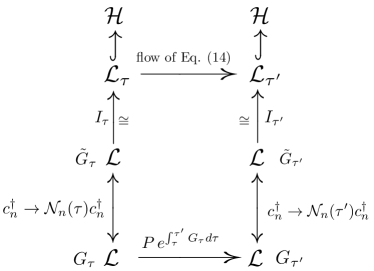
Figure 2: Commuting diagram displaying the various Hilbert spaces and sub-spaces defined in the main text, and operators acting between them. The top segment shows lowest Landau levels $\cal L_{\tau}$, $\cal L_{\tau^{\prime}}$ at different modular parameter that, using the 2D to 1D mapping defined in the text, have been embedded into the same larger 1D Hilbert space $\cal H$. At the same time, each Landau level is isomorphic (through embeddings $I_{\tau}$, $I_{\tau^{\prime}}$) to the same finite dimensional “abstract” Landau level space $\cal L$, in which only the guiding center degrees of freedom are represented. The generator $\tilde{G}_{\tau}$ of changes in the guiding center degrees of freedom with $\tau$ is first constructed using the normalization conventions of the 1D Hilbert space. It is related by a similarity transformation to the operator $G_{\tau}$, which generates the analogous changes for the normalization convention of the usual 2D Hilbert space. In the horizontal direction, we have mappings between states defined for values of the modular parameter. The upper line is defined through the flow of Eq. (14), which describes precisely the change of the Laughlin state, restricted to the real axis. The lower line represents the corresponding change in guiding center degrees of freedom, given by Eq. (41). The operator $G_{\tau}$ is constructed such that the diagram commutes.

If we perform this projection orthogonally with respect to the 1D scalar product, we obtain a ket

$$|\tilde{\psi}_{1/q}(\tau)\rangle=\sum_{\{n_{k}\}}\tilde{C}_{\{n_{k}\}}(\tau)c_{n_{1}}^{\dagger}\dotsc c_{n_{N}}^{\dagger}|0\rangle\,.$$ (17)

By definition, we then have

$$\nabla_{\tau}|\tilde{\psi}_{1/q}(\tau)\rangle=\tilde{{\bf G}}_{\tau}|\tilde{\psi}_{1/q}(\tau)\rangle\,,$$ (18)

where we assume $\tilde{{\bf G}}_{\tau}=(\tilde{G}_{\tau_{x}},\tilde{G}_{\tau_{y}})$ to be of the form

$$\tilde{{\bf G}}_{\tau}=\sum_{mm^{\prime}nn^{\prime}}{{\bf G}}_{mm^{\prime}nn^{\prime}}c_{m}^{\dagger}c_{m^{\prime}}^{\dagger}c_{n}c_{n^{\prime}}\,.$$ (19)

In the end, one wants to do the projection of Eq. (16) orthogonally with respect to the original 2D scalar product. This gives

$$|\psi_{1/q}(\tau)\rangle=\sum_{\{n_{k}\}}C_{\{n_{k}\}}(\tau)c_{n_{1}}^{\dagger}\dotsc c_{n_{N}}^{\dagger}|0\rangle$$ (20)

where $C_{\{n_{k}\}}={\cal N}_{n_{1}}\dotsc{\cal N}_{n_{N}}\tilde{C}_{\{n_{k}\}}$ from the change of normalization, $c_{n}^{\dagger}\rightarrow{\cal N}_{n}c_{n}^{\dagger}$. This implies the relation

$$|\psi_{1/q}(\tau)\rangle=e^{\sum_{n=0}^{L-1}\ln[{\cal N}_{n}(\tau)]c^{\dagger}_{n}c_{n}}|\tilde{\psi}_{1/q}(\tau)\rangle\,.$$ (21)

From this last line, we obtain that the desired operator ${{\bf G}}_{\tau}$ defined by Eq. (12) is related to Eq. (19) via

$${{\bf G}}_{\tau} =\sum_{n}\frac{\nabla_{\tau}{\cal N}_{n}(\tau)}{{\cal N}_{n}(\tau)}c^{\dagger}_{n}c_{n}$$

$$+\sum_{mm^{\prime}nn^{\prime}}\frac{{\cal N}_{m}(\tau){\cal N}_{m^{\prime}}(\tau)}{{\cal N}_{n}(\tau){\cal N}_{n^{\prime}}(\tau)}{{\bf G}}_{mm^{\prime}nn^{\prime}}\,c_{m}^{\dagger}c_{m^{\prime}}^{\dagger}c_{n}c_{n^{\prime}}.$$ (22)

With this we have completely relegated the solution of the problem to the 1D Hilbert space. We point out that the 1D mapping described above may generally provide an efficient way to calculate the matrix elements of operators acting within the lowest Landau level on the torus. In this case, Eq. (II.5) will apply without the $\tau$-derivative part. The explicit form of ${\cal N}_{n}(\tau)$ will be given below.

We now define the operator $I_{\tau}$ which injects the ket $|\tilde{\psi}_{1/q}(\tau)\rangle$ into ${\cal L}_{\tau}\in\cal H$, by sending $c^{\dagger}_{n}|0\rangle$ to $\tilde{\chi}_{n}(\tau)$. Thus

$$\psi_{1/q}=I_{\tau}|\tilde{\psi}_{1/q}\rangle\,.$$ (23)

For the time being, we work at fixed $\tau_{x}$. Using the heat equation (14) with $\partial_{\tau}=-i\partial_{\tau_{y}}$ and differentiating Eq. (23), one obtains

$$\partial_{\tau_{y}}\psi_{1/q}=i\Delta\psi_{1/q}=(\partial_{\tau_{y}}I_{\tau})|\tilde{\psi}_{1/q}\rangle+I_{\tau}\,\tilde{G}_{\tau_{y}}|\tilde{\psi}_{1/q}\rangle\,,$$ (24)

where $\Delta$ denotes the differential operator on the right hand side of Eq. (14), and we also used Eq. (18).

For $\mbox{Re}\,\tau=\mbox{Re}\,\tau^{\prime}$, it is easy to see the $P_{\tau}\partial_{\tau_{y}}I_{\tau}\equiv 0$, where $P_{\tau}$ is the orthogonal projection operator onto ${\cal L}_{\tau}$ (we work in the 1D Hilbert space now, and will always refer to its scalar product when not stated otherwise). To see this, it is sufficient to observe that $\langle\chi_{m}|\partial_{\tau_{y}}\chi_{n}\rangle=0$ for all $m$, $n$. This follows from the fact that $\langle\chi_{m}(\tau)|\chi_{n}(\tau^{\prime})\rangle=\delta_{m,n}\langle\chi_{m}(\tau)|\chi_{m}(\tau^{\prime})\rangle$ is always real for $\mbox{Re}\,\tau=\mbox{Re}\,\tau^{\prime}$. Thus, acting on the last equation with $P_{\tau}$, we get

$$P_{\tau}\Delta P_{\tau}\psi_{1/q}=P_{\tau}\Delta P_{\tau}I_{\tau}|\psi_{1/q}\rangle=I_{\tau}\tilde{G}_{\tau_{y}}|\tilde{\psi}_{1/q}\rangle\,.$$

where we have also inserted $P_{\tau}$ before $\psi_{1/q}\in{\cal L}_{\tau}$. Since we only care about how the operator $\tilde{G}_{\tau_{y}}$ acts on these $q$ states, for which we have the last equation, we may thus define this operator though the identity

$$\tilde{G}_{\tau_{y}}=I^{-1}_{\tau}P_{\tau}\Delta P_{\tau}I_{\tau}\,.$$ (25)

The last equation expresses that the matrix elements of $\tilde{G}_{\tau_{y}}$ are just those of the differential operator $\Delta$ restricted to the LLL subspace ${\cal L}_{\tau}$. These can thus be calculated straightforwardly by evaluating the standard expression for two-body operators:

$$G^{y}_{mm^{\prime}nn^{\prime}}=\frac{1}{2}\int_{0}^{1}dx\int_{0}^{1}dx^{\prime}\,\tilde{\chi}_{m}^{\ast}(x)\tilde{\chi}_{m^{\prime}}^{\ast}(x^{\prime})\;\Delta\;\tilde{\chi}_{n^{\prime}}^{\ast}(x^{\prime})\tilde{\chi}_{n}^{\ast}(x)\,.$$ (26)

As a last step, we calculate $G_{\tau_{y}}$ by fixing the normalization convention for single particle orbitals in accordance with the usual 2D scalar product, as displayed in Eq. (II.5). We may then obtain the generator for changes in $\tau_{x}$ simply by studying the analytic properties of the coefficients $C_{\{n_{k}\}}(\tau)$ in Eq. (20). As shown in Appendix A, one has

$$\partial_{\tau_{x}}C_{\{n_{k}\}}=-i\partial_{\tau_{y}}C_{\{n_{k}\}}+i\frac{N}{4\tau_{y}}\,.$$ (27)

We can thus let $G_{\tau_{x}}=-iG_{\tau_{y}}+i\frac{\hat{N}}{4\tau_{y}}$. Moreover, Eq. (27) follows from the fact that $C_{\{n_{k}\}}/\tau_{y}^{N/4}$ is holomorphic in $\tau$. We may use this insight to conveniently redefine the normalization of the Laughlin states via

$$\psi_{1/q}^{\prime\ell}(z_{1},\dotsc,z_{N},\tau)={\tau_{y}^{-N/4}}\,\psi_{1/q}^{\ell}(z_{1},\dotsc,z_{N},\tau)\,.$$ (28)

The corresponding generator for changes in $\tau_{y}$ is then given by $G^{\prime}_{\tau_{y}}=G_{\tau_{y}}-\frac{\hat{N}}{4\tau_{y}}$. In the following, we will always refer to the normalization convention (28). Dropping all primes, we then have

$$G_{\tau_{x}}=-iG_{\tau_{y}}\equiv G_{\tau}\,.$$ (29)

With the ket $|\psi_{1/q}(\tau)\rangle$ now referring to Eq. (28), $|\psi_{1/q}(\tau)\rangle$ is then holomorphic in $\tau$, and we have

$$\partial_{\tau}|\psi_{1/q}(\tau)\rangle=G_{\tau}|\psi_{1/q}(\tau)\rangle\,.$$ (30)

We present our final result as

$$G_{\tau}=G_{0}+\frac{1}{4\pi iq}G_{1}+qG_{2}\;.$$ (31)

Here, the first term corresponds to $-i$ times the one-body operator in the $y$-component of Eq. (II.5), plus the shift of $iN/4\tau_{y}$ shown in Eq. (27). Defining the functions

$${\cal S}_{n}^{a}=\sum_{l}(2\pi i[lL+n])^{a}e^{-2\pi L\tau_{y}(l+n/L)^{2}}\,,$$ (32)

the normalization factors defined above correspond to $({\cal N}_{n})^{-2}=\sqrt{2L/\tau_{y}}{\cal S}_{n}^{0}$. We thus get

$$G_{0}=\frac{i}{2}\sum_{n}\frac{\partial_{\tau_{y}}{\cal S}^{0}_{n}}{{\cal S}_{n}^{0}}\,c_{n}^{\dagger}c_{n}=-\frac{1}{4\pi iL}\sum_{n}\frac{{\cal S}^{2}_{n}}{{\cal S}_{n}^{0}}\,c_{n}^{\dagger}c_{n}\;.$$ (33)

Next, $G_{1}$ is the contribution coming from the differential operator $\partial_{X}^{2}$ in Eq. (14). Note that after normal ordering, the square of a single body operator still contains a single body operator. We thus get the following result:

$$G_{1}=(\frac{q}{L})^{2}[\sum_{n}\frac{{\cal S}^{2}_{n}}{{\cal S}^{0}_{n}}c_{n}^{\dagger}c_{n}+\sum_{n_{1}\neq n_{2}}\frac{{\cal S}^{1}_{n_{1}}{\cal S}^{1}_{n_{2}}}{{\cal S}^{0}_{n_{1}}{\cal S}^{0}_{n_{2}}}c_{n_{1}}^{\dagger}c_{n_{1}}c_{n_{2}}^{\dagger}c_{n_{2}}]\,.$$ (34)

Note that ${\cal S}^{2}_{n}\neq({\cal S}^{1}_{n})^{2}$, owing to the fact that $P_{\tau}\partial_{X}^{2}P_{\tau}\neq(P_{\tau}\partial_{X}P_{\tau})^{2}$. Finally, $G_{2}$ relates to the $\theta$-function part of Eq. (14). Eq. (26) can be evaluated by expanding the factors in the integrand, which are all periodic in $x$, $x^{\prime}$, into Fourier series. For the $\partial\theta/\theta$-terms, this can be done by contour integration and using known properties of $\theta$ functions. Straightforward but tedious calculation allows one to express $G_{2}$ through rapidly converging, albeit multiple sums,

$$G_{2}=\frac{1}{2}\sum_{n_{1}n_{2}n_{3}n_{4}}\frac{\Delta_{n_{1}n_{2}n_{3}n_{4}}}{{\cal S}_{n_{1}}^{0}{\cal S}_{n_{2}}^{0}}c_{n_{1}}^{\dagger}c_{n_{2}}^{\dagger}c_{n_{4}}c_{n_{3}}+\frac{1}{2}C\hat{N}(\hat{N}-1)\,,$$ (35)

and we have defined the function

$$\begin{split}\Delta_{n_{1}n_{2}n_{3}n_{4}}&=\delta_{n_{1}+n_{2},n_{3}+n_{4}}\frac{2\pi}{i}\sum_{\begin{subarray}{c}n\neq 0\\ n=n_{3}-n_{1}\mod L\end{subarray}}(\frac{e^{i\pi\tau n}}{1-e^{2i\pi\tau n}})^{2}\\ &\sum_{l_{1}}e^{i\pi\tau L[(n_{1}+n)/L+l_{1}]^{2}}(e^{i\pi\tau L(n_{1}/L+l_{1})^{2}})^{*}\\ &\sum_{l_{4}}(e^{i\pi\tau L[(n_{4}+n)/L+l_{4}]^{2}})^{*}e^{i\pi\tau L(n_{4}/L+l_{4})^{2}}\,,\end{split}$$ (36)

and the ($\tau$-dependent) constant

$$C=\frac{1}{4\pi i}[\int_{-1/2}^{1/2}(\frac{\partial_{\tau}\theta_{4}}{\theta_{4}})^{2}dz-\pi^{2}]\,.$$ (37)

In the above, the Kronecker $\delta$ is understood to be periodic, enforcing identity $n_{1}+n_{2}=n_{3}+n_{4}\mod\;L$.

II.6 Symmetry considerations

The operator $G_{\tau}$ defined in the preceding section is manifestly invariant under magnetic translations in the $x$-direction. In the basis we chose here, this is tantamount to the conservation, modulo $L$, of the “center-of-mass” operator $\sum_{n}nc^{\dagger}_{n}c_{n}$. On the other hand, the operator is not invariant under magnetic translations in the $\tau$-direction, which amounts to an ordinary shift of the orbital indices. As already pointed out in Sec. II.2, the symmetrized operator

$$G_{\tau,\mbox{\tiny sym}}=\frac{1}{L}\sum_{n=0}^{L-1}T_{\tau}^{n}\,G_{\tau}(T_{\tau}^{\dagger})^{n}$$ (38)

also satisfies Eq. (12), where $T_{\tau}$ generates magnetic translations in $\tau$. This is a trivial consequence of the fact that the $|\psi_{1/q}^{\ell}(\tau)\rangle$ transform among themselves under $T_{\tau}$, and all satisfy Eq. (12). Likewise, each term on the right hand side of Eq. (38) satisfies Eq. (12). We may thus define the $L-1$ linearly independent 2-body operators

$$D_{n}=G_{\tau,\mbox{\tiny sym}}-T_{\tau}^{n}\,G_{\tau}(T_{\tau}^{\dagger})^{n},\quad n=0\dotsc L-2,$$ (39)

that all annihilate each of the $q$-fold degenerate Laughlin states,

$$D_{n}|\psi_{1/q}^{\ell}\rangle=0\;.$$ (40)

We note that the $D_{n}$ are not in any obvious way related to the operators $Q^{\dagger}_{R}Q_{R}$ of the pseudo-potential Hamiltonian, with $Q_{R}$ given by (9). Indeed, the $D_{n}$ have a non-vanishing single-body term, whereas the $Q^{\dagger}_{R}Q_{R}$ do not. The $D_{n}$ thus represent a new class of two-body operators that annihilate the torus Laughlin states (in the absence of quasi-holes). For $q=3$ and various values of particle number $N$, we have verified that the property (39) characterizes the $q=3$ Laughlin states uniquely.

Note that the single-body contribution to $G_{\tau,\mbox{\tiny sym}}$ is proportional to the particle number, as explained in Sec. II.2. This term can thus be replaced by a constant when acting on the Laughlin state, and hence can be ignored altogether in practical calculations, where the real part of this constant is usually adjusted to fix the normalization of the state (see below), and the imaginary part only affects the phase convention. For the same reason, we do not need the value of the $\tau$-dependent constant $C$ defined in Eq. (37) for the purpose of practical calculations.

II.7 Presentation of the Laughlin state through its thin torus limit

In the following, we will generally identify $G_{\tau}$ with the symmetrized operator $G_{\tau,\mbox{\tiny sym}}$ discussed in the preceding section, without carrying along the ”sym” label. Putting the results of Sec. II.5 in integral form, we have, via Eq. (30),

$$|\psi_{1/q}^{\ell}(\tau^{\prime})\rangle=P\,e^{\int_{\tau}^{\tau^{\prime}}G_{\tau}d\tau}\,|\psi_{1/q}^{\ell}(\tau)\rangle\,,$$ (41)

where $P$ means path ordering. The integral in Eq. (41) should be interpreted as a complex contour integral, where the result is independent of the path connecting $\tau$ and $\tau^{\prime}$. This is so since by construction, $G_{\tau}$ generates exactly the change with $\tau$ of the guiding center coordinates of the states in Eq. (28), which are single valued functions of $\tau$. (This requires that we carry along all the $\tau$-dependent c-number terms mentioned in the preceding section.)

We may also want to add, possibly different, real constants to $G_{\tau_{x}}$ and $G_{\tau_{y}}$, such that the normalization of the Laughlin state is preserved under the evolution with these operators. When evaluating Eq. (41) iteratively, this simply corresponds to normalizing the state at each step. We denote the accordingly modified operators by $G_{\tau_{x}}^{N}$ and $G_{\tau_{y}}^{N}$, and introduce the operator valued 1-form $dG^{N}_{\tau}=G_{\tau_{x}}^{N}d\tau_{x}+G_{\tau_{y}}^{N}d\tau_{y}$. We may then write

$$|\psi_{1/q}^{\ell}(\tau^{\prime})\rangle_{N}=P\,e^{\int_{\tau}^{\tau^{\prime}}dG_{\tau}^{N}}\,|\psi_{1/q}^{\ell}(\tau)\rangle_{N}\,,$$ (42)

where the subscript $N$ denotes normalized Laughlin states. We are now interested in the thin torus limit $\tau\rightarrow i\infty$, in which $|\psi_{1/3}^{\ell}(\tau)\rangle_{N}$ approaches the ket $|100100100\dotsc\rangle$,Seidel et al. (2005) or one related to the latter through repeated action of $T_{\tau}$. Here, the labels 100100100…are occupation numbers in the basis (15). Given our earlier discussion for the cylinder, it cannot be taken for granted that Eq. (42) remains well-defined in this limit. On the other hand, it may seem plausible that this is the case, since the operators $G_{\tau_{x}}^{N}$, $G_{\tau_{y}}^{N}$ do generate off-diagonal matrix elements when acting on the thin torus state, unlike the case of the cylinder. It thus seems feasible that the full Laughlin states at arbitrary $\tau$ admit the following presentation in terms of their respective thin torus limit,

$$|\psi_{1/q}^{\ell}(\tau)\rangle_{N}=P\,e^{\int_{\infty}^{\tau}dG_{\tau}^{N}}|...100...100...100...\dotsc\rangle\,,$$ (43)

where the pattern on the right hand side denotes one of the $q$ thin torus patterns at filling factor $1/q$. The correctness of the above assertion remains non-trivial, however, as the $\tau^{\prime}\rightarrow\infty$ limit in Eq. (42) must be taken with care. In the next Section we provide numerical evidence for $q=3$, demonstrating the above relation for various particle numbers $N$. We thus find that the full torus Laughlin state may be generated from its given thin torus limit via application of the above path-ordered exponential involving the two-body operator constructed here. We conjecture that this is true for general $q$. An application demonstrating this technique will be discussed in the following.

III Application: Hall viscosity

As an application of our findings in Sec. II, we use Eq. (43) (or the differential form Eq. (30)) to calculate the $\nu=1/3$ torus Laughlin state along a contour in the complex $\tau$-plane, starting from the thin torus limit at $\tau=i\infty$. As a physical motivation for calculating the Laughlin state along such contours, we will be asking how the Hall viscosityRead (2009) evolves along such contours. This quantity is naturally related to the main theme of of our paper, i.e., changes of the Laughlin state with changes in geometry. The notion of a Hall viscosity of fractional quantum Hall liquids has generated much interest recently,Read (2009); Haldane (2009); Read and Rezayi (2011) expanding earlier workAvron et al. (1995) on integer quantum Hall states. In particular, in an insightful paper, Read (2009) Read has derived a general relation between the viscosity of a quantum Hall fluid and a characteristic quantum number $\bar{s}$, which can be interpreted as “orbital spin per particle” and is related to the conformal field theory description of the state in question. Here we only give a brief summary of the relevant definitions, following closely Ref. Read and Rezayi, 2011, to which we refer the interested reader for details.

We denote the fourth-rank viscosity tensor of the fluid by $\eta_{abcd}$, where we are interested in the case of two spatial dimensions. In a situation with no dissipation, only its anti-symmetric or “Hall viscosity” component $\eta^{(A)}_{abcd}=-\eta^{(A)}_{cdab}$ may be non-zero, and this is possible only when time reversal symmetry and the symmetry under reflection of space are both broken. This is the situation in a magnetic field (where in a constant field, only the product of these two symmetries is unbroken).

We now consider a system with periodic boundary conditions defined by two periods ${\bf L}_{1}=(L_{1},0)$ and ${\bf L}_{2}=(L_{1}\tau_{x},L_{1}\tau_{y})$, and Hamiltonian

$$\begin{split}H=\frac{1}{2}\sum_{i=1}^{N}&g^{ab}\pi_{ia}\pi_{ib}\,+\\ &P_{\mbox{\tiny LLL}}\,\sum_{m,n}\sum_{i<j}V(||x_{ij}+m{{\bf L}}_{1}+n{{\bf L}_{2}}||_{g})\,P_{\mbox{\tiny LLL}}\end{split}$$ (44)

Here, $\pi_{a}$ is a component of the kinetic momentum, $P_{\mbox{\tiny LLL}}$ denotes LLL-projection, and we have introduced a metric $g_{ab}$. We have also introduced the “periodized” version of a potential $V$ that depends on $x_{i}$, $x_{j}$ only via $||x_{ij}||_{g}\equiv g_{ab}x_{ij}^{a}x_{ij}^{b}$ with $x_{ij}=x_{i}-x_{j}$. We follow Ref. Read and Rezayi, 2011 and parametrize the metric via $g(\lambda)=\Lambda^{T}\Lambda$, $\Lambda=\exp(\lambda)$, where $\Lambda$ can be viewed as a coordinate transformation that transforms the identity metric into the metric $g$. Clearly, $g$ is invariant under $\Lambda\rightarrow R\Lambda$, where $R$ is a rotation matrix. Since $\lambda$ can be interpreted as being proportional to an “infinitesimal version” of $\Lambda$, whose rotational component is just its anti-symmetric part, we may fix this rotational degree of freedom by requiring $\lambda$ to be symmetric. Then, the Hall viscosity of the ground state of Eq. (44) can be relatedAvron et al. (1995); Read and Rezayi (2011); Bradlyn et al. (2012) to the adiabatic curvature on the space of background metrics, here parameterized by the symmetric matrix $\lambda$. Specializing to $g=\mbox{id}$, we have:

$$\eta^{(A)}_{abcd}=-\frac{1}{V}F_{ab;cd}$$ (45)

where $F_{ab;cd}$ is the Berry curvature

$$F_{ab;cd}=-2\mbox{Im}\langle\partial_{\lambda_{ab}}\psi|\partial_{\lambda_{cd}}\psi\rangle|_{g=\mbox{id}}\;,$$ (46)

and $\psi$ denotes the ground state of Eq. (44). $F_{ab;cd}$ clearly has the anti-symmetry of $\eta^{(A)}_{abcd}$, and it is also symmetric in the index pairs $ab$ and $cd$. Furthermore, at least in the thermodynamic limit of large $L_{1}$, one would expect $\eta^{(A)}_{abcd}$ to acquire full rotational symmetry. In two dimensions, this requires the trace $\eta^{(A)}_{abcc}$ to vanish, where we use the sum convention, and similarly for the first index pair. (In higher dimensions, rotational symmetry requires $\eta^{(A)}$ to vanish identically). Moreover, in an incompressible fluid, the strain tensor $u_{ab}$ must be traceless. Therefore, since the viscosity couples to the rate of strain $\dot{u}_{ab}$ via $\eta^{(A)}_{abcd}\dot{u}_{cd}$ to give a viscous contribution to the stress tensor, only the traceless part of $\eta^{(A)}_{abcd}$ is of interest. It therefore makes sense to restrict our attention to traceless $\lambda_{ab}$, corresponding to volume preserving coordinate transformations. Requiring $F_{ab;cd}$ thus to be anti-symmetric, symmetric in the first and second pair, as well as traceless, in $D=2$ the associated curvature 2-form $F=\frac{1}{2}F_{ab;cd}\,d\lambda_{ab}\wedge d\lambda_{cd}$ can only depend on the following two independent linear combinations of 1-forms, $d\lambda_{11}-d\lambda_{22}$ and $d\lambda_{12}+d\lambda_{21}$. Hence it must be proportional to their product:Read and Rezayi (2011)

$$F=-\frac{1}{2}s\,(d\lambda_{11}-d\lambda_{22})\wedge(d\lambda_{12}+d\lambda_{21})\,,$$ (47)

and we introduced a proportionality factor $-s/2$ whose physical meaning will be given below. The above expression in Eq. (45) gives

$$\eta^{(A)}_{abcd}=\eta^{(A)}(\delta_{ad}\epsilon_{bc}+\delta_{bc}\epsilon_{ad})$$ (48)

with

$$\eta^{(A)}=\frac{1}{2}\bar{s}\bar{n}\hbar\;,$$ (49)

where $\bar{n}=N/V$ is the particle density, $\bar{s}=s/N$, and we have restored a factor of $\hbar$. As shown in Ref. Read, 2009, in the thermodynamic limit the parameter $\bar{s}$ is quantized and can be identified with the average orbital spin per particle, which is related to the conformal dimension of the field describing particles in the conformal field theory description of the state. It is further related to the topological shift on the sphere, $\cal S$, of the underlying state via $\bar{s}={\cal S}/2$. For the Laughlin $1/3$ state, $\bar{s}=3/2$.

We now consider fixed boundary conditions described by $\tau$, and introduce a metric that corresponds to the infinitesimal transformation

$$d\lambda=\frac{1}{2\tau_{y}}\begin{pmatrix}-d\tau_{y}&d\tau_{x}\\ d\tau_{x}&d\tau_{y}\end{pmatrix}\,.$$ (50)

It is not difficult to see that the corresponding metric change is equivalent to changing the modular parameter $\tau$ to $\tau^{\prime}=\tau+d\tau_{x}+id\tau_{y}$. We may thus rewrite Eq. (47) as

$$F=-\frac{N\bar{s}}{2\tau_{y}^{2}}\,d\tau_{x}\wedge d\tau_{y}\,.$$ (51)

To each $\lambda$ can be associated a $\tau^{\prime}$, where $\Lambda=\exp(\lambda)$ is the coordinate transformation that changes the $\tau$-boundary condition into a $\tau^{\prime}$-boundary condition, where

$$\tau^{\prime}=\frac{\Lambda{\bf L}_{1}\cdot\Lambda{\bf L}_{2}+i\Lambda{\bf L}_{1}\times\Lambda{\bf L}_{2}}{||\Lambda{\bf L}_{1}||^{2}}\,.$$ (52)

For fixed $\tau$, we now parameterize $\lambda$, and thus the metric, by $\tau^{\prime}$. (Note that the right hand side of Eq. (52) can be viewed as a function of $\Lambda$ and $\tau$.) Eq. (51) then implies that

$$\bar{s}=\frac{4\tau_{y}^{2}}{N}\,\mbox{Im}\,\langle\partial_{\tau^{\prime}_{x}}\psi|\partial_{\tau^{\prime}_{y}}\psi\rangle\,.$$ (53)

We emphasize that in the above, $\psi\equiv\psi(\tau,g_{\tau}(\tau^{\prime}))$ always satisfies the same boundary condition defined by $\tau$, and depends on $\tau^{\prime}$ only through the metric. At the same time, $\psi(\tau,g_{\tau}(\tau^{\prime}))$ is related to $\psi(\tau^{\prime},\mbox{id})$ by the unitary transformation $\chi_{n}(\tau,g_{\tau}(\tau^{\prime}))\rightarrow\chi_{n}(\tau^{\prime},\mbox{id})$, with $\chi_{n}(\tau,g(\tau^{\prime}))$ the deformed version of the state (15) in the presence of the metric $g(\tau^{\prime})$. However, for fixed $\tau$, the $\psi(\tau,g_{\tau}(\tau^{\prime}))$ live in the same Hilbert space,Read and Rezayi (2011) independent of $\tau^{\prime}$. The advantage of introducing both $\tau$ and $\tau^{\prime}$, where the former describes boundary conditions, and the latter describes the “true geometry” of the system, is that we may restrict ourselves to metrics $g_{\tau}(\tau^{\prime})$ in the vicinity of the identity (corresponding to $\tau^{\prime}$ close to $\tau$), such that Eq. (45) is directly applicable.

We now consider $\psi=\psi^{N}_{1/3}$, the normalized Laughlin $1/3$ state (where we suppress labels $\tau$, $\tau^{\prime}$, and $\ell$). We have the expansion

$$\psi_{1/3}^{N}=\sum_{\{n_{k}\}}C^{N}_{\{n_{k}\}}(\tau^{\prime})|{\{n_{k}\}}\rangle_{g}\,,$$ (54)

and $|{\{n_{k}\}}\rangle_{g}\rangle$ is short for the Slater determinant ${\cal A}\,\left[\chi_{n_{1}}(z_{1},\tau,g(\tau^{\prime}))\cdot\dotsc\cdot\chi_{n_{N}}(z_{N},\tau,g(\tau^{\prime}))\right]$. We write $-2\mbox{Im}\,\langle\partial_{\tau^{\prime}_{x}}\psi|\partial_{\tau^{\prime}_{y}}\psi\rangle=\nabla_{\tau^{\prime}}\times A$ where

$$A=i\sum_{\{n_{k}\}}\,\left(|C^{N}_{\{n_{k}\}}|^{2}~{}_{g}\langle{\{n_{k}\}}|\nabla_{\tau^{\prime}}|{\{n_{k}\}}\rangle_{g}+{C^{N}}^{*}_{\!\!\!\!\!\!\{n_{k}\}}\nabla_{\tau^{\prime}}C^{N}_{\{n_{k}\}}\right)$$ (55)

is the Berry connection. It turns out that in the first term, which describes the change of the LLL basis with $\tau^{\prime}$, $~{}_{g}\langle{\{n_{k}\}}|\nabla_{\tau^{\prime}}|{\{n_{k}\}}\rangle_{g}$ is independent of $\{n_{k}\}$, and contributes a constant $1/2$ to Eq. (53).Lévay (1995) The second term depends on the changes of the $C_{\{n_{k}\}}$ with $\tau^{\prime}$, which we described in the preceding section. We first assume the general situation where this change is described by Eq. (12) with two generators $G_{\tau_{x}}$ and $G_{\tau_{y}}$ that are not necessarily related and that do not necessarily preserve the normalization of the state. It is straightforward to show that the contribution from the second term then leads to the following connected expectation value,

$$\begin{split}&-2\,\mbox{Im}\sum_{\{n_{k}\}}\partial_{\tau^{\prime}_{x}}{C^{N}}^{\ast}_{\!\!\!\!\!\!\{n_{k}\}}\partial_{\tau^{\prime}_{y}}C^{N}_{\{n_{k}\}}\\ &=i\left[\langle G_{\tau_{x}}^{\dagger}G_{\tau_{y}}-G_{\tau_{y}}^{\dagger}G_{\tau_{x}}\rangle-\langle G_{\tau_{x}}^{\dagger}\rangle\langle G_{\tau_{y}}\rangle+\langle G_{\tau_{y}}^{\dagger}\rangle\langle G_{\tau_{x}}\rangle\right]\,,\end{split}$$ (56)

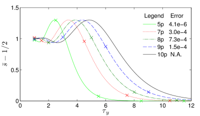
Figure 3: Average “orbital spin per particle” $\bar{s}$ as calculated from Eq. (53), for the $\nu=1/3$ torus Laughlin state at $\tau$ generated via Eq. (58), using the procedure described in the main text and below. We start with the thin torus state at relatively large but finite $\tau^{\prime}$, and iteratively solve Eq. (30) using the 4th order Runge-Kutta method. Final state errors compared with exact diagonalization at $\tau=i$ are shown for 5 particles for $\tau^{\prime}=30i$ and step size $d\tau=0.01i$, 7 and 8 particles for $\tau^{\prime}=30i$ and $d\tau=0.05i$, 9 particles for $\tau^{\prime}=40i$, $d\tau=0.025i$. 10 particles data is shown for $\tau^{\prime}=80i$, $d\tau=0.02i$. Crosses denote the value of $\bar{s}-1/2$ obtained from the exactly diagonalized Laughlin state in Eq. (53), for comparison. The errors of $\bar{s}$ are at or smaller than $10^{-6}$ in these cases. All the errors decrease further with larger initial $\tau^{\prime}$ and smaller step size.

where expectation values on the right hand side are taken in the state Eq. (54). The last two terms take care of the normalization, and will cancel if both operators are anti-Hermitian (describing unitary evolution), in which case the expression reduces to the expectation value of a commutator. Note also that the expression is invariant under constant shifts of any of the two operators. We now specialize to the case where these operators are related by Eq. (29). Plugging Eq. (55), Eq. (56) into Eq. (53), this gives

$$\bar{s}=\frac{1}{2}+\frac{4\tau_{y}^{2}}{N}|\Delta G_{\tau}|^{2}\,,$$ (57)

where $|\Delta G_{\tau}|=(\langle G_{\tau}^{\dagger}G_{\tau}\rangle-\langle G_{\tau}^{\dagger}\rangle\langle G_{\tau}\rangle)^{1/2}$ is the variance of the operator $G_{\tau}$ in the state $\psi^{N}_{1/3}$, and is manifestly positive (the Laughlin state at $\tau$ certainly being no eigenstate of $G_{\tau}$ for any $\tau$). As stated above, for the Laughlin state $\bar{s}$ is expected to approach $3/2$ in the thermodynamic limit. This has been checked in Ref. Read and Rezayi, 2011, by calculating torus Laughlin (and other) states by exact diagonalization of parent Hamiltonians, and computing the Berry curvature by taking overlaps between such states for different $\tau$ (or $\lambda$). Here we will consider the same problem both as a demonstration and a consistency check of the results presented in the preceding section. To this end, we calculate the Laughlin state from the presentation (43), or by numerically integrating the differential equation (30) with thin torus initial conditions, and then computing $\bar{s}$ from Eq. (57). Note that both steps of the calculation make use of the two-body operator $G_{\tau}$. In particular, our results will confirm the accuracy of Eq. (43), which may be written more carefully as

$$|\psi_{1/q}^{\ell}(\tau)\rangle_{N}=\lim_{\tau^{\prime}\rightarrow i\infty}P\,e^{\int_{\tau^{\prime}}^{\tau}dG_{\tau}^{N}}|...100...100...100...\dotsc\rangle\,.$$ (58)

Evaluating the expression on the right for some large but finite $\tau^{\prime}$ is equivalent to integrating Eq. (30) (and normalizing the result), where the thin torus limiting state defines the initial condition at $\tau^{\prime}$. This obviously introduces some error compared to the full Laughlin state at the initial value $\tau^{\prime}$, hence also at the final value $\tau$. Since it is not clear a priori how this error behaves in the limit of large imaginary $\tau^{\prime}$, possible pitfalls are that the limit in Eq. (58) is ill-defined, or that it is well-defined but does not agree with the Laughlin state. Our results, however, give strong support of Eq. (58).

Fig. 3 shows the results for the value of $\bar{s}-1/2$ from this method for $q=3$. Beginning with the thin torus state $|100100100\dotsc\rangle$ at large imaginary $\tau^{\prime}$, we evolve the state down to $\tau=i$, i.e., a torus of aspect ratio 1, integrating Eq. (30) using the classical 4th order Runge-Kutta method. We normalize the state at each step. For particle numbers $N=5$ to $N=9$, we have observed that the error of the state obtained at $\tau=i$, compared to the Laughlin state generated from exact diagonalization of the $V_{1}$ Haldane pseudopotential, $|\psi-\psi_{ed}|$, becomes systematically smaller with increasing initial $\tau^{\prime}$ and decreasing step size $d\tau$. The observed state error at $\tau=i$ has been on the order of $10^{-6}$ for $N=5$, $d\tau=0.01i$, and $\tau^{\prime}=30$, and on the order of $10^{-4}$ for $N=9$, $d\tau=0.025i$, and $\tau^{\prime}=40$. For $N=10$, we show data based on our method only. Generally, larger $N$ requires larger $\tau^{\prime}$ for the same accuracy. Fig. 3 shows $\bar{s}-1/2$ for various $N$ using our method, whereas crosses denote isolated points for which values have been obtained from exact diagonalization for comparison. One sees that the expected value of $\bar{s}-1/2=1$ is always approached rather closely for $\tau=i$, though it deviates from this value for $|\tau|$ noticeably larger than $1$. The crossover where notable deviations from $1$ set in is pushed to larger $|\tau|$ with increased particle number, as expected. However, the value of $\bar{s}$ is found to be much more constant, and close to its expected thermodynamic limit, when instead of varying the modulus of $\tau$ we vary its phase at $|\tau|=1$, even for five particles, as shown in Fig. 4. Data were obtained by continued integration of Eq. (30) away from $\tau=i$ along a contour where $\tau=\exp(i\theta)$. $\bar{s}-1/2$ remains close to $1$ except for angles $\theta$ approaching $\pi$. These observations are consistent with the exact diagonalization data published in Ref. Read and Rezayi, 2011 for $N=10$ and (at $\tau=\exp(i\pi/3)$) larger particle number.

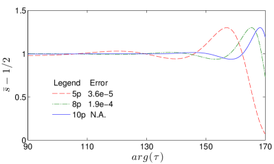
Figure 4: Average orbital spin per particle $\bar{s}$, calculated from Eq. (53), for the $\nu=1/3$ torus Laughlin state. The state has been evolved out of the thin torus limit first down to $\tau=i$ as described in the caption of Fig. 3, and then to $\tau=e^{i\theta}$ using the same method. The step sizes used are $d\theta=0.01rad$ for 5 particles and $d\theta=0.001rad$ for 8 and 10 particles. The state difference with the exactly diagonalized Laughlin state at the last step is listed in the figure. Data stay close to the value $\bar{s}-1/2=1$ expected in the thermodynamic limitRead (2009) for a wide range of angles $\theta$, as first observed in Ref. Read and Rezayi, 2011 from exact diagonalization.

IV Discussion

In the preceding sections, we considered the change in the guiding center variables, with modular parameter $\tau$ for the torus Laughlin states. Within a given Landau level, the guiding center coordinates fully specify the state. We have shown that this change is generated by a two-body operator $G_{\tau}$, which we have explicitly constructed. We have demonstrated numerically that by means of this two-body operator, the Laughlin state for any modular parameter $\tau$ can be generated from its simple thin torus ($\tau=i\infty$) limit. The ability to generate the full torus Laughlin state in this way may be compared to squeezing rules that follow from the Jack polynomial structure of this state in other geometries.Bernevig and Haldane (2008a, b) From a practical point of view, however, our method still requires integration of a first order differential equation. While this requires some compromise between accuracy and computational effort, the added benefit is that in the process of the calculation, the Laughlin state is generated along an entire contour in the complex $\tau$ plane, rather than just for a single value of $\tau$. It is thus likely that whenever a moderate error can be tolerated, but many $\tau$ values are of interest, our method may become competitive compared to numerical diagonalization. As a demonstration of these features, we have produced results relating to the Hall viscosity that are similar to those of Ref. Read and Rezayi, 2011 (and are expected to be identical within numerical accuracy for identical particle number, which we have not yet studied). The Hall viscosity is itself deeply related to our main theme of study, i.e., geometric changes in the Laughlin state,Avron et al. (1995); Read (2009); Read and Rezayi (2011) and we have discussed its precise relation to the generator constructed here (Eq. (57)), following Ref. Read and Rezayi, 2011.

We note that one key ingredient of our procedure is to embed different torus Laughlin states, which are related to one another by the application of strain, into the same Hilbert space. For this we make use of a dimensional reduction that is made possible by the analytic properties of lowest Landau level wave functions on the torus. We argued that this mapping may be useful in other contexts. However, recent work on Hall viscosityRead and Rezayi (2011) achieves the same embedding by a different method, which is to introduce a metric describing the effect of strain, rather than a change in boundary conditions. We conjecture that if we had used this method in Sec. II, we would have directly obtained the symmetrized version of our operator $G_{\tau}$. In this way, however, we would not have obtained the family of two-body operators given in Sec. II.6, whose members annihilate the torus Laughlin states.

While primarily, we have been working in a finite dimensional Hilbert space that represents guiding center-coordinates only, the operator defined in Sec. II also naturally acts within the full Hilbert space, which can be viewed as the tensor product of the degrees of freedom for the guiding centers and the dynamical momenta, respectively. Within this larger, physical, Hilbert space, the operator $G_{\tau}$ generates the change in guiding center degrees of freedom associated to a change in the torus geometry, but not the corresponding change of the Landau level. As pointed out recently by Haldane,Haldane (2011) the Laughlin state may be generalized by the introduction of a geometric parameter that describes the deformation of guiding center variables in response to a change in the “interaction metric”. The so deformed Laughlin state is still the exact ground state of an appropriately deformed Hamiltonian. The operator that we have constructed can thus also be viewed as generating the change of the torus Laughlin state in response to a change of the interaction metric, i.e., the change in ground state for the corresponding family of deformed pseudo-potential Hamiltonians. For the disc geometry, this problem has been addressed from different angles previously.Read and Rezayi (2011); Qiu et al. (2012)

We conjecture that the observations made here are not limited to Laughlin states, but can be generalized to other quantum Hall states as well. Indeed, a great wealth of model wave functions is obtained from conformal blocks in rational conformal field theories.Moore and Read (1991) For conformal blocks on the torus, the dependence on the modular parameter $\tau$ can be described by Knizhnik-Zamolodchikov-Bernard (KZB) type equations.Bernard (1988) We expect therefore that our approach can be generalized to other trial wave functions related to conformal field theories. The details of such generalizations are left for future work.

V Conclusion

In this work, we have shown that geometric changes in the guiding center coordinates of the torus Laughlin state are generated by a two-body operator. We have demonstrated that the equation that governs the evolution of the torus Laughlin state as a function of the modular parameter $\tau$ can be continued into the thin torus limit. This gives rise to a new presentation of the torus Laughlin state in its second quantized, or guiding center, form. This presentation allows one to calculate the torus Laughlin states in terms of a simple thin torus or “dominance” pattern by means of integration of the flow generated by the two-body operator defined in this work. This operator hence realizes the adiabatic evolution of the simple thin torus product state into the full Laughlin state on regular tori. To demonstrate this, we have numerically compared both the Laughlin state generated from this method, as well as the Hall viscosity derived from it, to exact diagonalization results. While the demonstration of our new presentation of the torus Laughlin state rests in part on numerics, we defer more detailed analytic studies to future investigation.

Appendix A Analytic properties of coefficients

For definiteness, we will refer to the Laughlin state $\psi_{1/q}^{\ell}$ using the normalization conventions (6), (7). The coefficients $C_{\{n_{k}\}}(\tau)$ defined in Eq. (20) then imply the following expansion of the analytic Laughlin state,

$$\psi^{\ell}_{1/q}(\tau)=\sum_{\{n_{k}\}}C_{\{n_{k}\}}(\tau)\,{\cal A}\,\chi_{n_{1}}(z_{1},\tau)\cdot\dotsc\cdot\chi_{n_{N}}(z_{N},\tau)\,.$$ (59)

Here, as before, the symbol $\cal A$ denotes anti-symmetrization, and single particle orbitals $\chi_{n}$ are defined in Eq. (15). We define new orbitals $\chi_{n}^{\prime}(\tau)=\tau_{y}^{1/4}\chi_{n}(\tau)$ that are holomorphic in $\tau$, as is the Laughlin state $\psi_{1/q}^{\ell}(\tau)$. Hence, by acting with $\partial_{\bar{\tau}}=\frac{1}{2}(\partial_{\tau_{x}}+i\partial_{\tau_{y}})$ on Eq. (59), we obtain

$$0=\sum_{\{n_{k}\}}\left[\partial_{\bar{\tau}}\left(C_{\{n_{k}\}}(\tau)/\tau_{y}^{N/4}\right)\right]\,{\cal A}\,\chi^{\prime}_{n_{1}}(z_{1},\tau)\cdot\dotsc\cdot\chi^{\prime}_{n_{N}}(z_{N},\tau)\,.$$ (60)

The linear independence of the orbitals $\chi_{n}^{\prime}(\tau)$ and of the associated many-particle Slater determinants then implies

$$\partial_{\bar{\tau}}\left(C_{\{n_{k}\}}(\tau)/\tau_{y}^{N/4}\right)=0\,,$$ (61)

i.e., the quantities $C_{\{n_{k}\}}(\tau)/\tau_{y}^{N/4}$ are holomorphic in $\tau$. Eq. (27) follows immediately from Eq. (61).

References

- Tsui et al. (1982) D. C. Tsui, H. L. Stormer, and A. C. Gossard, Physical Review Letters 48, 1559 (1982).
- Laughlin (1983) R. B. Laughlin, Physical Review Letters 50, 1395 (1983).
- Moore and Read (1991) G. Moore and N. Read, Nuclear Physics B 360, 362 (1991).
- Read and Rezayi (1999) N. Read and E. Rezayi, Physical Review B 59, 8084 (1999).
- Haldane and Rezayi (1988) F. D. M. Haldane and E. H. Rezayi, Physical Review Letters 60, 956 (1988).
- Halperin (1983) B. Halperin, Helvetica Physica Acta 56, 75 (1983).
- Simon et al. (2007) S. H. Simon, E. H. Rezayi, N. R. Cooper, and I. Berdnikov, Physical Review B 75, 075317 (2007).
- Jain (1989) J. K. Jain, Phys. Rev. Lett. 63, 199 (1989).
- Haldane (1983) F. D. M. Haldane, Physical Review Letters 51, 605 (1983).
- Trugman and Kivelson (1985) S. A. Trugman and S. Kivelson, Physical Review B 31, 5280 (1985).
- Greiter et al. (1991) M. Greiter, X.-G. Wen, and F. Wilczek, Physical Review Letters 66, 3205 (1991).
- Note (1) By this we mean that the ground state is exactly known.
- MacDonald (1994) A. H. MacDonald, arXiv:cond-mat/9410047 (1994).
- Rezayi and Haldane (1994) E. H. Rezayi and F. D. M. Haldane, Physical Review B 50, 17199 (1994).
- Lee and Leinaas (2004) D.-H. Lee and J. M. Leinaas, Phys. Rev. Lett. 92, 096401 (2004).
- Qi (2011) X.-L. Qi, Physical Review Letters 107, 126803 (2011).
- Wang and Scarola (2011) H. Wang and V. W. Scarola, Physical Review B 83, 245109 (2011).
- Seidel et al. (2005) A. Seidel, H. Fu, D.-H. Lee, J. M. Leinaas, and J. Moore, Physical Review Letters 95, 266405 (2005).
- Haldane (2011) F. D. M. Haldane, Physical Review Letters 107, 116801 (2011).
- Qiu et al. (2012) R.-Z. Qiu, F. D. M. Haldane, X. Wan, K. Yang, and S. Yi, Physical Review B 85, 115308 (2012).
- Note (2) We note though a tractable truncated version of Eq. (3) with matrix product ground state given in Ref. \rev@citealpnumBergholtz12.
- Bernevig and Haldane (2008a) B. A. Bernevig and F. D. M. Haldane, Physical Review Letters 100, 246802 (2008a).
- Bernevig and Haldane (2008b) B. A. Bernevig and F. D. M. Haldane, Physical Review B 77, 184502 (2008b).
- Haldane and Rezayi (1985) F. D. M. Haldane and E. H. Rezayi, Physical Review B 31, 2529 (1985).
- Wen and Niu (1990) X. G. Wen and Q. Niu, Physical Review B 41, 9377 (1990).
- Read and Rezayi (1996) N. Read and E. Rezayi, Physical Review B 54, 16864 (1996).
- Bergholtz and Karlhede (2005) E. J. Bergholtz and A. Karlhede, Physcal Review Letters 94, 26802 (2005).
- Seidel and Lee (2006) A. Seidel and D.-H. Lee, Physical Review Letters 97, 056804 (2006).
- Bergholtz and Karlhede (2006) E. J. Bergholtz and A. Karlhede, J. Stat. Mech. L04001 (2006).
- Seidel and Lee (2007) A. Seidel and D.-H. Lee, Phys. Rev. B 76, 155101 (2007).
- Seidel (2008) A. Seidel, Physical Review Letters 101, 196802 (2008).
- Flavin and Seidel (2011) J. Flavin and A. Seidel, Physical Review X 1, 021015 (2011).
- Flavin et al. (2012) J. Flavin, R. Thomale, and A. Seidel, Physical Review B 86, 125316 (2012).
- Seidel and Yang (2011) A. Seidel and K. Yang, Physical Review B 84, 085122 (2011).
- Read (2009) N. Read, Physical Review B 79, 045308 (2009).
- Note (3) Indeed, as formulated at present, these different Landau levels do not even live in the same Hilbert space, since the domain of the underlying wave functions depends on the value of . This is inconsequential at present, however, and will later be remedied.
- Read and Rezayi (2011) N. Read and E. H. Rezayi, Physical Review B 84, 085316 (2011).
- Seidel (2010) A. Seidel, Physical Review Letters 105, 026802 (2010).
- Note (4) It turns out that the final form of also contains a one body part that we omit in (19\@@italiccorr), (II.5\@@italiccorr) for brevity. However this part transforms analogously.
- Note (5) We are indebted to G. Möller for this observation.
- Haldane (2009) F. D. M. Haldane, arXiv:0906.1854 (2009).
- Avron et al. (1995) J. E. Avron, R. Seiler, and P. G. Zograf, Physical Review Letters 75, 697 (1995).
- Bradlyn et al. (2012) B. Bradlyn, M. Goldstein, and N. Read, Physical Review B 86, 245309 (2012).
- Lévay (1995) P. Lévay, Journal of Mathematical Physics 36, 2792 (1995).
- Note (6) The latter case is obviously realized for the Laughlin state on the cylinder and the operator defined in Sec. II.1, where the expression analogous to the right hand side Eq. (58) leaves the thin torus limiting state invariant.
- Bernard (1988) D. Bernard, Nuclear Physics B 303, 77 (1988).
- Nakamura et al. (2012) M. Nakamura, Z.-Y. Wang, and E. J. Bergholtz, Physical Review Letters 109, 016401 (2012).