Recent progress in calculation of $B_{K}$ using staggered fermions

Abstract:

We report on recent progress in the calculation of $B_{K}$ using HYP-smeared improved staggered fermions on the MILC asqtad lattices. We have added measurements on fine ($a\sim 0.09\;$fm) and superfine ($a\sim 0.06\;$fm) ensembles at different values of the light sea quark mass ($am_{\ell}$), as well as increased the statistics on some other ensembles. We find that the results on the fine lattices show a significantly stronger $am_{\ell}$ dependence than those on the superfine and coarse ($a\sim 0.12\;$fm) lattices. We discuss different methods for accounting for these new results when doing the $am_{\ell}$ and continuum extrapolations.

1 Introduction

The calculation of the kaon mixing matrix element $B_{K}$ is one of the successes of lattice QCD. Results with all errors controlled are available with several fermion discretizations [1, 2]. The value for $B_{K}$ is a key input into the standard model prediction for $\epsilon_{K}$. At present there is an $\approx 3\sigma$ tension between this prediction and the experimental value (if one uses the “exclusive” $V_{cb}$ obtained using lattice QCD) [5, 6, 7]. Thus it is important to continue to further improve the lattice calculations.

In this proceedings we provide an update on our results for $B_{K}$. These are obtained using improved staggered fermions, specifically HYP-smeared valence quarks on asqtad sea-quarks. We describe here results obtained using chiral extrapolations based on SU(2) staggered chiral perturbation theory (SChPT), which is our most reliable procedure [3, 4]. Details of the fitting functions and the analysis method are given in Ref. [3, 4], and are not repeated here.

Table 1 lists all the ensembles on which we have calculated $B_{K}$, and notes which results have changed in the last year. In particular, since Lattice 2011 we have accumulated much higher statistics on the F2 and S1 ensembles (in addition to a small increase on the U1 ensemble) and added new measurements on ensembles F3, S2 and S3. Of these, the most important updates are those on ensembles F2, F3, S2, and S3, since they give information on the light sea quark mass dependence which was previously lacking on the fine and superfine ensembles. We focus on this dependence here.

$a$ (fm)	$am_{l}/am_{s}$	geometry	ID	ens $\times$ meas	status
0.12	0.03/0.05	$20^{3}\times 64$	C1	$564\times 9$	old
0.12	0.02/0.05	$20^{3}\times 64$	C2	$486\times 9$	old
0.12	0.01/0.05	$20^{3}\times 64$	C3	$671\times 9$	old
0.12	0.01/0.05	$28^{3}\times 64$	C3-2	$275\times 8$	old
0.12	0.007/0.05	$20^{3}\times 64$	C4	$651\times 10$	old
0.12	0.005/0.05	$24^{3}\times 64$	C5	$509\times 9$	old
0.09	0.0093/0.031	$28^{3}\times 96$	F3	$949\times 9$	new
0.09	0.0062/0.031	$28^{3}\times 96$	F1	$995\times 9$	old
0.09	0.0031/0.031	$40^{3}\times 96$	F2	$959\times 9$	update
0.06	0.0072/0.018	$48^{3}\times 144$	S3	$593\times 9$	new
0.06	0.0036/0.018	$48^{3}\times 144$	S1	$749\times 9$	update
0.06	0.0025/0.018	$56^{3}\times 144$	S2	$799\times 9$	new
0.045	0.0028/0.014	$64^{3}\times 192$	U1	$747\times 1$	update

Table 1: MILC asqtad ensembles used to calculate $B_{K}$. $am_{\ell}$ and $am_{s}$ are the masses, in lattice units, of the light and strange sea quarks, respectively. “ens” indicates the number of configurations on which “meas” measurements are made. Note that the numbering of the ID tags on the fine and superfine lattices do not follow the ordering of $am_{\ell}$.

2 Chiral fits

In our numerical study, our lattice kaons are composed of valence (anti)quarks with masses $m_{x}$ and $m_{y}$. These are, respectively, the masses of the valence $d$ and $s$ quarks. On each MILC ensemble, we use 10 valence masses:

$$am_{x},am_{y}=am_{s}\times{n}/{10}\qquad\text{with}\qquad n=1,2,3,\ldots,10,$$ (1)

where $am_{s}$ is the nominal strange sea quark mass. In our standard fits we extrapolate to $am_{d}^{\rm phys}$ using the lowest 4 values for $am_{x}$ (the “X-fit”—done at fixed $am_{y}$), and then extrapolate to $m^{\textrm{phys}}_{s}$ using the highest 3 values of $am_{y}$ (“Y-fit”). As described in Ref. [3], these choices keep us in the regime where we expect next-to-leading order (NLO) SU(2) ChPT to be reasonably accurate. The X-fits described here are done to the form predicted by NLO partially quenched SChPT (which is given in Refs. [3, 8]), augmented by analytic and generic non-analytic terms of next-to-next-to-leading order (NNLO) and a single analytic term of next-to-next-to-next-to-leading order (NNNLO). We use the Bayesian method to constrain the higher order coefficients, as described in Refs. [3, 4, 9]. The $am_{y}$ dependence (which is not controlled by ChPT) is very close to linear and we use a linear fit for our central values. We dub this entire fitting procedure the “4X3Y-NNNLO fit”, and use it for our central values.

(a) F3

(b) F2

Figure 1: X-fits to $B_{K}(1/a)$ for the F3 and F2 ensembles. The red diamond is explained in the text.

(a) S3

(b) S2

Figure 2: X-fits to $B_{K}(1/a)$ for the S3 and S2 ensembles. Notation as in Fig. 1.

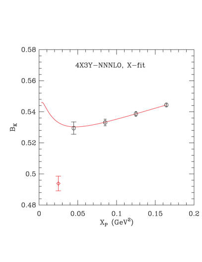
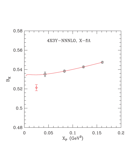
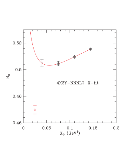
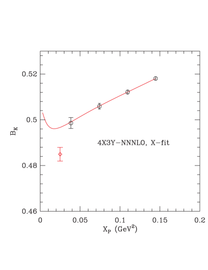
The X-fits on the new fine ensembles are shown in Fig. 1, while those on the new superfine ensembles are shown in Fig. 2. In each panel, a fit to the SU(2) SChPT form is shown, with $X_{P}$ the squared-mass of the Goldstone-taste valence $\bar{x}x$ pion, whose mass is very close to linear to $am_{x}$. Also shown (as the red diamond) is the result obtained after (a) extrapolating $am_{x}\to am_{d}^{\rm phys}$, (b) removing the known taste-breaking in the pion masses appearing in the chiral logarithms, and (c) setting the light sea-quark mass to its physical value in the chiral logarithmic terms. See Ref. [3] for details of this procedure. We have incorporated finite volume corrections, as predicted by NLO SChPT, into the fitting function [10].

A notable feature of both figures is that the difference between the extrapolated/corrected result and the fit curve is larger on the ensembles with larger $am_{\ell}$ (F3 and S3). This is due almost entirely to the larger shift required to bring the sea-quark pion mass to its physical value on these lattices (correction (c) above). The other aspects of the extrapolation/correction are similar for the pairs of lattices. We return to this point below.

3 Dependence On Light Sea Quark Mass

Figure 3: $B_{K}(\mu=2\,\text{GeV})$ vs. $L_{P}\,(\text{GeV}^{2})$, where $L_{P}$ is a squared mass of the Goldstone-taste pion composed of two light sea quarks ($\bar{\ell}\ell$).

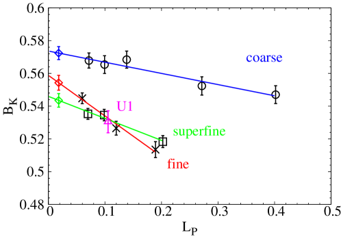
In Fig. 3, we show the dependence of $B_{K}$ on the light sea quark mass for all lattice spacings, including the U1 point for completeness. We use $L_{P}$ as a proxy for $am_{\ell}$, since these quantities are proportional to very good accuracy. We have run $B_{K}$ to a common renormalization scale $\mu=2\,\text{GeV}$ (in the $\overline{\rm MS}$ scheme), so that the results are directly comparable. We expect, at NLO, only a linear behavior on $L_{P}$.

As can be seen from the plot, a linear fit works well for each of the three lattice spacings for which we have multiple values of $am_{\ell}$. The results on the coarse lattices, which were presented in Ref. [4], show a mild dependence on $L_{P}$. The slope, $-1/(2.9\;{\rm GeV})^{2}$, is consistent with naive dimensional analysis, which predicts a magnitude of ${\cal O}(1/\Lambda_{\chi}^{2})$ with $\Lambda_{\chi}\approx 1\;$GeV. The slope on the superfine lattices, which is a new result, has a slightly larger magnitude than that on the coarse lattices but is comparable. What is striking, however, is the slope on the fine lattices, whose magnitude is about twice that on the coarse lattices (slope $\approx-1/(2\;{\rm GeV})^{2}$). Its value per se is reasonable—what is unexpected is that it should differ so much from that at the other lattice spacings. Since we are in the regime where corrections are small ($\leq 10\%$) in both chiral and continuum extrapolations, one would expect that the slope would depend only weakly on $a^{2}$, and any dependence should be linear. Instead, our results appear to require a contribution to $B_{K}$ proportional to $am_{\ell}(a^{2})^{2}$, since only with a quadratic dependence on $a^{2}$ can the magnitude of the slope increase and then decrease as $a^{2}$ is raised.

This peculiar behavior has only recently come to light and we are in the process of investigating it. One avenue we are following is to do a global continuum-chiral extrapolation to all results. This would incorporate the constraint that fit parameters in the chiral fits should depend smoothly on $a^{2}$. Another approach is to remove the step (c) described above from our correction procedure and leave this to be dealt with by the $am_{\ell}$ extrapolation. This is possible because, at NLO in SChPT, $L_{P}$ does not appear in the argument of the chiral logarithms, but only in the prefactor. Pending a more complete understanding, we have considered the continuum extrapolation of results obtained after the extrapolation to physical $am_{\ell}$.

4 Continuum Extrapolation

In Fig. 4, we show the results obtained on the coarse, fine and superfine lattices after the linear extrapolation to $am_{\ell}^{\rm phys}$ plotted vs. $a^{2}$. We also include the U1 result which, however, is not extrapolated to physical $am_{\ell}$, since there is only one value of $am_{\ell}$ available for the ultrafine lattices. Thus it cannot be consistently used in the continuum extrapolation.

Figure 4: $B_{K}(\mu=2\,\text{GeV})$ vs. $a^{2}\,(100\times\text{fm}^{2})$. See text for description of data points. Note that the U1 point (smallest $a^{2}$) has not been extrapolated to physical $am_{\ell}$. Red, brown and blue curves and points show the lin3, lin4 and g4-a2g2-a4 fits, respectively.

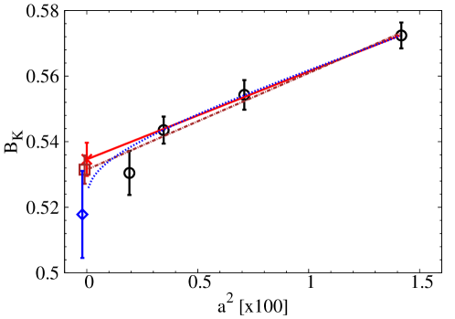
Previously, when the high-statistics data from ensembles F2, F3, S2 and S3 were not available, we made the continuum extrapolation using ensembles C3, F1, S1 and U1, all of which have close to the same sea-quark masses. We then included systematic errors accounting for the use of unphysical sea-quark masses (the errors being 1.5% and 1.3% for the light and strange sea-quark masses, respectively [4]). We found a continuum behavior which was far from linear in $a^{2}$ (as can be seen from Fig. 3—the fit corresponds to $L_{P}\approx 0.1\;{\rm GeV}^{2}$), and we could not obtain reasonable fits including the coarse ensemble. Dropping this, and trying various fits (along the lines described below) we estimated an extrapolation error of 1.9%.

Using the data extrapolated to physical $am_{\ell}$ leads to a much smoother continuum extrapolation, as can be seen in Fig. 4. We can now obtain good fits including the coarse lattice result. As noted above, we can consistently fit only to the larger three values of $a^{2}$. Following Ref. [4], we fit both to a linear dependence and to a five-parameter form containing dependence that we know enters due to incomplete operator matching and higher-order contributions. The explicit forms are given in Table 2, For the five-parameter fit we use Bayesian constraints for $c_{2}-c_{5}$, with central values set to zero and spreads taken as $\sigma_{2}=\sigma_{3}=\sigma_{5}=2\Lambda^{2}$ and $\sigma_{4}=2$, with $\Lambda=300\;$MeV. These fits are shown in Fig. 4; values for $\chi^{2}/\text{d.o.f.}$ and extrapolated $B_{K}$ are listed in the Table. Also shown, for completeness, is a linear fit including the U1 point, labeled lin4.

fit type	# data	fit function	$\chi^{2}$/d.o.f.	$B_{K}(2\;{\rm GeV})$
lin3	3	$c_{1}+c_{2}a^{2}$	0.0307	0.5346(51)
g4-a2g2-a4	3	$c_{1}+c_{2}a^{2}+c_{3}a^{2}\alpha_{s}(a)$
		$+c_{4}\alpha_{s}^{2}(a)+c_{5}a^{4}$	0.0298	0.5178(133)
lin4	4	$c_{1}+c_{2}a^{2}$	0.703	0.5314(43)

Table 2: Details of continuum fits. For the g4-a2g2-a4 fit with Bayesian constraints, the augmented $\chi^{2}$/d.o.f. is shown. Only statistical errors are shown for $B_{K}$.

At this stage we are not ready to quote an updated result for $B_{K}$, since we clearly need to improve our understanding of the $am_{\ell}$ dependence. Nevertheless, we note that, taking the linear continuum extrapolation (fit lin3) the final value for $\widehat{B}_{K}$ is $0.732$ with a $\sim 1\%$ statistical error. This is, in fact, consistent with our previous result of $0.727\pm 0.038$ [4] (where the error is dominated by systematics). Setting aside the matching error of 4.4%, we note that the combined $am_{\ell}$ and continuum extrapolation systematics were estimated at 2.4%. This is certainly large enough to accommodate any small shift we might find from our new analysis. Thus we do not expect a significant change in our final result. We do hope, however, that the $am_{\ell}$ extrapolation error will come down. The total error will, at present, remain dominated by the matching error (due to our use of 1-loop perturbative matching).

In summary, results at different light sea-quark masses on the fine and superfine MILC asqtad ensembles have uncovered an $am_{\ell}$ dependence that is hard to understand. An optimistic interpretation of the new results is that the difficulties we had previously when extrapolating at unphysical $am_{\ell}$ were due to artifacts introduced by our X-fitting and extrapolation procedure, while the new continuum fits (shown in Fig. 4) do not contain these artifacts. Analysis is underway to test this interpretation, and final results should be available soon.

5 Acknowledgments

We are grateful to Claude Bernard and the MILC collaboration for private communications. C. Jung is supported by the US DOE under contract DE-AC02-98CH10886. The research of W. Lee is supported by the Creative Research Initiatives Program (2012-0000241) of the NRF grant funded by the Korean government (MEST). W. Lee would like to acknowledge the support from KISTI supercomputing center through the strategic support program for the supercomputing application research [No. KSC-2011-G2-06]. The work of S. Sharpe is supported in part by the US DOE grant no. DE-FG02-96ER40956. Computations were carried out in part on QCDOC computing facilities of the USQCD Collaboration at Brookhaven National Lab, on GPU computing facilities at Jefferson Lab, on the DAVID GPU clusters at Seoul National University, and on the KISTI supercomputers. The USQCD Collaboration are funded by the Office of Science of the U.S. Department of Energy.

References

- [1] G. Colangelo et al., FLAG Collaboration, Eur. Phys. J. C71, 1695 (2011). [arXiv:1011.4408].
- [2] Lattice Averages web site, http://krone.physik.unizh.ch/l̃unghi/webpage/LatAves/.
- [3] Taegil Bae, et al., SWME Collaboration, Phys. Rev. D82, (2010), 114509 [arXiv:1008.5179].
- [4] Taegil Bae, et al., SWME Collaboration, Phys. Rev. Lett. 109, (2012), 041601 [arXiv:1111.5698].
- [5] Jack Laiho, Ruth S. Van de Water, Enrico Lunghi, Phys. Rev. D81, (2010) 034503; [arXiv:0910.2928].
- [6] Enrico Lunghi, Amarjit Soni, Phys. Lett. B697, (2011), 323; [arXiv:1010.6069].
- [7] Yong-Chull Jang and Weonjong Lee, SWME Collaboration, PoS (Lattice 2012) 269; [arXiv:1211.0792].
- [8] R.S. Van de Water and S.R. Sharpe, Phys. Rev. D73 (2006) 014003 [hep-lat/0507012].
- [9] Boram Yoon, et al., SWME Collaboration, [arXiv:1101.2248].
- [10] Jangho Kim, et al., SWME Collaboration, Phys. Rev. D83, (2011), 117501 [arXiv:1101.2685].
- [11] Jon Bailey, et al., FNAL/MILC Collaboration Phys. Rev. D85 (2012) 114502 [arXiv:1202.6346].