Image denoising with multi-layer perceptrons, part 1:
comparison with existing algorithms and with bounds
Abstract
Image denoising can be described as the problem of mapping from a noisy image to a noise-free image. The best currently available denoising methods approximate this mapping with cleverly engineered algorithms. In this work we attempt to learn this mapping directly with plain multi layer perceptrons (MLP) applied to image patches. We will show that by training on large image databases we are able to outperform the current state-of-the-art image denoising methods. In addition, our method achieves results that are superior to one type of theoretical bound and goes a large way toward closing the gap with a second type of theoretical bound. Our approach is easily adapted to less extensively studied types of noise, such as mixed Poisson-Gaussian noise, JPEG artifacts, salt-and-pepper noise and noise resembling stripes, for which we achieve excellent results as well. We will show that combining a block-matching procedure with MLPs can further improve the results on certain images. In a second paper (Burger et al., 2012b), we detail the training trade-offs and the inner mechanisms of our MLPs.
Keywords: Multi-layer perceptrons, image denoising, Gaussian noise, mixed Poisson-Gaussin noise, JPEG artifacts
1 Introduction
 |
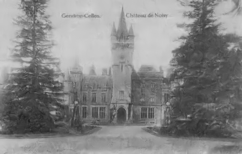 |
| Noisy castle | Clean castle |
Images are invariably corrupted by some degree of noise. The strength and type of noise corrupting the image depends on the imaging process. In scientific imaging, one sometimes needs to take images in a low photon-count setting, in which case the images are corrupted by mixed Poisson-Gaussian noise (Luisier et al., 2011). Magnetic resonance images are usually corrupted by noise distributed according to the Rice disitribution (Gudbjartsson and Patz, 1995). For natural images captured by a digital camera, the noise is usually assumed to be additive, white and Gaussian-distributed (AWG noise), see for example Elad and Aharon (2006); Dabov et al. (2007).
An image denoising procedure takes a noisy image as input and estimates an image where the noise has been reduced. Numerous and diverse approaches exist: Some selectively smooth parts of a noisy image (Tomasi and Manduchi, 1998; Weickert, 1998). Other methods rely on the careful shrinkage of wavelet coefficients (Simoncelli and Adelson, 1996; Portilla et al., 2003). A conceptually similar approach is to denoise image patches by trying to approximate noisy patches using a sparse linear combination of elements of a learned dictionary (Aharon et al., 2006; Elad and Aharon, 2006). BM3D (Dabov et al., 2007) is a very successful approach to denoising and is often considered state-of-the art. The approach does not rely on a probabilistic image prior but rather exploits the fact that images are often self-similar: A given patch in an image is likely to be found elsewhere in the same image. In BM3D, several similar-looking patches of a noisy image are denoised simultaneously and collaboratively: Each noisy patch helps to denoise the other noisy patches. The algorithm does not rely on learning from a large dataset of natural images; excellent denoising results are achieved through the design of the algorithm. While BM3D is a well-engineered algorithm, could we also automatically learn an image denoising procedure purely from training examples consisting of pairs of noisy and noise-free patches?
Denoising as a function:
In image denoising, one is given a noisy version of a clean image, where the noise is for instance i.i.d. Gaussian distributed with known variance (AWG noise). The goal is to find the clean image, given only the noisy image. We think of denoising as a function that maps a noisy image to a cleaner version of that image. However, the complexity of a mapping from images to images is large, so in practice we chop the image into possibly overlapping patches and learn a mapping from a noisy patch to a clean patch. To denoise a given image, all image patches are denoised separately by that map. The denoised image patches are then combined into a denoised image.
The size of the patches affects the quality of the denoising function. If the patches are small and the noise level is high, many clean patches are a potential explanation for a given noisy patch. In other words, adding noise to a clean patch is not injective and therefore also not invertible. It is therefore almost impossible to find a perfect denoising function. Lowering the noise and increasing the size of the patches alleviates this problem: Fewer clean patches are a potential explanation for a given noisy image (Levin and Nadler, 2011). At least in theory, better denoising results are therefore achievable with large patches than with small patches.
In practice, the mapping from noisy to clean patches cannot be expressed using a simple formula. However, one can easily generate samples: Adding noise to a patch creates an argument-value pair, where the noisy patch is the argument of the function and the noise-free patch is the value of the function.
The aim of this paper is to learn the denoising function. For this, we require a model. The choice of the model is influenced by the function to approximate. Complicated functions require models with high capacity, whereas simple functions can be approximated using a model with low capacity. The dimensionality of the problem, which is defined by the size of the patches, is one measure of the difficulty of approximation. One should therefore expect that models with more capacity are required when large image patches are used. A higher dimensionality also usually implies that more training data is required to learn the model, unless the problem is intrinsically of low dimension.
We see that a trade-off is necessary: Very small patches lead to a function that is easily modeled, but to bad denoising results. Very large patches potentially lead to better denoising results, but the function might be difficult to model.
This paper will show that it is indeed possible to achieve state-of-the-art denoising performance with a plain multi layer perceptron (MLP) that maps noisy patches onto noise-free ones. This is possible because the following factors are combined:
-
•
The capacity of the MLP is chosen large enough, meaning that it consists of enough hidden layers with sufficiently many hidden units.
-
•
The patch size is chosen large enough, so that a patch contains enough information to recover a noise-free version. This is in agreement with previous findings (Levin and Nadler, 2011).
-
•
The chosen training set is large enough. Training examples are generated on the fly by corrupting noise-free patches with noise.
Training high capacity MLPs with large training sets is feasible using modern Graphics Processing Units (GPUs). Burger et al. (2012b) contains a detailed analysis of the trade-offs during training.
Contributions:
We present a patch-based denoising algorithm that is learned on a large dataset with a plain neural network. Additional contributions of this paper are the following.
-
1.
We show that the state-of-the-art is improved on AWG noise. This is done using a thorough evaluation on test images,
-
2.
excellent results are obtained on mixed Poisson-Gaussian noise, JPEG artifacts, salt-and-pepper noise and noise resembling stripes, and
-
3.
We present a novel “block-matching” multi-layer perceptron and discuss its strengths and weaknesses.
-
4.
We relate our results to recent theoretical work on the limits of denoising (Chatterjee and Milanfar, 2010; Levin and Nadler, 2011; Levin et al., 2012). We will show that two of the bounds described in these papers cannot be regarded as hard limits. We make important steps towards reaching the third proposed bound.
While we have previously shown that MLPs can achieve outstanding image denoising results (Burger et al., 2012a), in this work we present significantly improved results compared to our previous work as well as more thorough experiments.
2 Related work
The problem of removing noise from natural images has been extensively studied, so methods to denoise natural images are numerous and diverse. Estrada et al. (2009) classify denoising algorithms into three categories:
- 1.
- 2.
-
3.
The third class of denoising algorithms exploit learned image statistics. A natural image model is typically learned on a noise-free training set (such as the Berkeley segmentation dataset) and then exploited to denoise images (Roth and Black, 2009; Weiss and Freeman, 2007; Jain and Seung, 2008). In some cases, denoising might involve the careful shrinkage of coefficients. For example Simoncelli and Adelson (1996); Chang et al. (2002); Pizurica et al. (2002); Portilla et al. (2003) involve shrinkage of wavelet coefficients. Other methods denoise small images patches by representing them as sparse linear combinations of elements of a learned dictionary (Elad and Aharon, 2006; Mairal et al., 2008, 2010).
Neural networks:
Neural networks belong to the category relying on learned image statistics. They have already been used to denoise images (Jain and Seung, 2008) and belong in the category of learning-based approaches. The networks commonly used are of a special type, known as convolutional neural networks (CNNs) (LeCun et al., 1998a), which have been shown to be effective for various tasks such as hand-written digit and traffic sign recognition (Sermanet and LeCun, 2011). CNNs exhibit a structure (local receptive fields) specifically designed for image data. This allows for a reduction of the number of parameters compared to plain multi layer perceptrons while still providing good results. This is useful when the amount of training data is small. On the other hand, multi layer perceptrons are potentially more powerful than CNNs: MLPs can be thought of as universal function approximators (Cybenko, 1989; Hornik et al., 1989; Funahashi, 1989; Leshno et al., 1993), whereas CNNs restrict the class of possible learned functions.
A different kind of neural network with a special architecture (containing a sparsifying logistic) is used in (Ranzato et al., 2007) to denoise image patches. A small training set is used. Results are reported for strong levels of noise. It has also been attempted to denoise images by applying multi layer perceptrons on wavelet coefficients (Zhang and Salari, 2005). The use of wavelet bases can be seen as an attempt to incorporate prior knowledge about images.
Denoising auto-encoders (Vincent et al., 2010) also use the idea of using neural networks for denoising. Denoising auto-encoders are a special type of neural network which can be trained in an unsupervised fashion. Interesting features are learned by the units in the hidden layers. For this, one exploits the fact that training pairs can be generated cheaply, by somehow corrupting (such as by adding noise to) the input. However, the goal of these networks is not to achieve state-of-the-art results in terms of denoising performance, but rather to learn representations of data that are useful for other tasks. Another difference is that typically, the noise used is not AWG noise, but salt-and-pepper noise or similar forms of noise which “occlude” part of the input. Denoising auto-encoders are learned layer-wise and then stacked, which has become the standard approach to deep learning (Hinton et al., 2006). The noise is applied on the output of the previously learned layer. This is different from our approach, in which the noise is always applied on the input patch only and all layers are learned simultaneously.
Our approach is reminiscent of deep learning approaches because we also employ several hidden layers. However, the goal of deep learning is to learn several levels of representations, corresponding to a hiearchy of features, see Bengio (2009) for an overview. In this work we are mainly interested in image denoising results.
Innovations in this work:
Most methods based on neural networks make assumptions about natural images. Instead, we show that state-of-the-art results can be obtained by imposing no such assumptions, but by relying on a pure learning approach.
3 Learning to denoise
In Section 1, we defined the denoising problem as learning the mapping from a noisy patch to a cleaner patch. For this, we require a model. In principle, different models could be used, but we will use MLPs for that purpose. We chose MLPs over other models because of their ability to handle large datasets.
3.1 Multi layer perceptrons (MLPs)
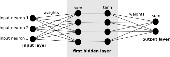
A multi layer perceptron (MLP) is a nonlinear function that maps vector-valued input via several hidden layers to vector-valued output. For instance, an MLP with two hidden layers can be written as,
| (1) |
The weight matrices and vector-valued biases parameterize the MLP, the function operates component-wise. The architecture of an MLP is defined by the number of hidden layers and by the layer sizes. For instance, a (256,2000,1000,10)-MLP has two hidden layers. The input layer is 256-dimensional, i.e. . The vector of the first hidden layer is 2000-dimensional, the vector of the second hidden layer is 1000-dimensional, and the vector of the output layer is 10-dimensional. Commonly, an MLP is also called feed-forward neural network. MLPs can also be represented graphically, see Figure 2. All our MLPs are fully connected, meaning that the weight matrices are dense. One could also imagine MLPs which are not fully connected, using sparse weight matrices. Sparsely connected MLPs have the advantage of being potentially computationally easier to train and evaluate.
MLPs belong to the class of parametric models, the parameters being estimated during learning. However, the number of parameters in MLPs is often so large that they are extremely flexible.
3.2 Training MLPs for image denoising
To train an MLP that maps noisy image patches onto clean image patches where the noise is reduced or even removed, we estimate the parameters by training on pairs of noisy and clean image patches using stochastic gradient descent (LeCun et al., 1998b).
More precisely, we randomly pick a clean patch from an image dataset and generate a corresponding noisy patch by corrupting with noise, for instance with additive white Gaussian (AWG) noise. We then feed the noisy patch into the MLP to compute , representing an estimate of the clean patch . The MLP parameters are then updated by the backpropagation algorithm (Rumelhart et al., 1986) minimizing the squared error between the mapped noisy patch and the clean patch , i.e. minimizing pixel-wise . We choose to minimize the mean squared error since it is monotonically related to the PSNR, which is the most commonly used measure of image quality. Thus minimizing the squared error will maximize PSNR values.
To make backpropagation efficient, we apply various common neural network tricks (LeCun et al., 1998b):
-
1.
Data normalization: The pixel values are transformed to have approximately mean zero and variance close to one. More precisely, assuming pixel values between and , we subtract and multiply by .
-
2.
Weight initialization: We use the “normalized initialization” described by Bengio and Glorot (2010). The weights are sampled from a uniform distribution:
(2) where and are the number of neurons in the input side and output side of the layer, respectively. Combined with the first trick, this ensures that both the linear and the non-linear parts of the sigmoid function are reached.
-
3.
Learning rate division: In each layer, we divide the learning rate by , the number of input units of that layer. This allows us to change the number of hidden units without modifying the learning rate.
The basic learning rate was set to for most experiments. The training procedure is discussed in more detail in Burger et al. (2012b).
3.3 Number of hidden layers
The number hidden layers as well as the number of neurons per hidden layer control the capacity of the model. No more than a single hidden layer is needed to approximate any function, provided that layer contains a sufficient number of neurons (Cybenko, 1989; Hornik et al., 1989; Funahashi, 1989; Leshno et al., 1993). However, functions exist that can be represented compactly with a neural network with hidden layers but that would require exponential size (with respect to input size) networks of depth (Håstad and Goldmann, 1991; Le Roux and Bengio, 2010). Therefore, in practice it is often more convenient to use a larger number of hidden layers with fewer hidden units each. The trade-off between a larger number of hidden layers and a larger number of hidden units is discussed in Burger et al. (2012b).
3.4 Applying MLPs for image denoising
To denoise images, we decompose a given noisy image into overlapping patches. We then normalize the patches by subtracting and dividing by , denoise each patch separately and perform the inverse normalization (multiply with , add ) on the denoised patches. The denoised image is obtained by placing the denoised patches at the locations of their noisy counterparts, then averaging on the overlapping regions. We found that we could improve results slightly by weighting the denoised patches with a Gaussian window. Also, instead of using all possible overlapping patches (stride size , or patch offset ), we found that results were almost equally good by using every third sliding-window patch (stride size ), while decreasing computation time by a factor of . Using a stride size of , we were able to denoise images of size pixels in approximately one minute (on CPU), which is slower than BM3D (Dabov et al., 2007), but much faster than KSVD (Aharon et al., 2006) and NLSC (Mairal et al., 2010) and also faster than EPLL (Zoran and Weiss, 2011).
3.5 Efficient implementation on GPU
The computationally most intensive operations in an MLP are the matrix-vector multiplications. For these operations Graphics Processing Units (GPUs) are better suited than Central Processing Units (CPUs) because of their ability to efficiently parallelize operations. For this reason we implemented our MLP on a GPU. We used nVidia’s C2050 GPU and achieved a speed-up factor of more than one order of magnitude compared to an implementation on a quad-core CPU. This speed-up is a crucial factor, allowing us to run larger-scale experiments. We describe training for various setups in Burger et al. (2012b).
4 Experimental setup
We performed all our experiments on gray-scale images. These were obtained from color images with matlab’s rbg2gray function. Since it is unlikely that two noise samples are identical, the amount of training data is effectively infinite, no matter which dataset is used. However, the number of uncorrupted patches is restricted by the size of the dataset. Note that the MLPs could be also trained on color images, possibly exploiting structure between the different color channels. However, in this publication we focus on the gray-scale case.
Training data:
For almost all our experiments, we used images from the imagenet dataset (Deng et al., 2009). Imagenet is a hiearchically organized image database, in which each node of the hierarchy is depicted by hundreds and thousands of images. We completely disregard all labels provided with the dataset. We used images from different object categories. We performed no pre-processing other than the transform to grey-scale on the training images.
Test data:
We define six different test sets to evaluate our approach:
-
1.
standard test images: This set of images contains standard images, such as “Lena” and “Barbara”, that have been used to evaluate other denoising algorithms (Dabov et al., 2007).
- 2.
-
3.
Pascal VOC 2007: We randomly selected images from the Pascal VOC 2007 test set (Everingham et al., 2007).
-
4.
Pascal VOC 2011: We randomly selected images from the Pascal VOC 2011 training set.
-
5.
McGill: We randomly selected images from the McGill dataset (Olmos et al., 2004).
-
6.
ImageNet: We randomly selected 500 images from the ImageNet dataset not present in the training set. We also used object categories not used in the training set.
We selected dataset 1) because it has become a standard test dataset, see Dabov et al. (2007) and Mairal et al. (2010). The images contained in it are well-known and diverse: Image “Barbara” contains a lot of regular structure, whereas image “Man” contains more irregular structure and image “Lena” contains smooth areas. We chose to make a more thorough comparison, which is why we evaluated our approach as well as competing algorithms on five larger test sets. We chose five different image sets of images instead of one set of images in order to see if the performance of methods is significantly affected by the choice of the dataset. EPLL (Zoran and Weiss, 2011) is trained on a subset of dataset 2), NLSC (Mairal et al., 2010) is trained on a subset of 4) and our method is trained on images extracted from the same larger dataset as 6).
Types of noise:
For most of our experiments, we used AWG noise with . However, we also show results for other noise levels. Finally, we trained MLPs to remove mixed Gaussian-Poisson noise, JPEG artifacts, salt and pepper noise and noise that resembles stripes.
5 Results: comparison with existing algorithms
In this section, we present results achieved with an MLP on AWG noise with five different noise levels. We also present results achieved on less well-studied forms of noise. We present in more detail what steps we took to achieve these results in Burger et al. (2012b).
We compare against the following algorithms:
-
1.
KSVD (Aharon et al., 2006): This is a dictionary-based method where the dictionary is adapted to the noisy image at hand. A noisy patch is denoised by approximating it with a sparse linear combination of dictionary elements.
-
2.
EPLL (Zoran and Weiss, 2011): The distribution of image patches is described by a mixture of Gaussians. The method presents a novel approach to denoising whole images based on patch-based priors. The method was shown to be sometimes superior to BM3D (Dabov et al., 2007), which is often considered the state-of-the-art in image denoising.
-
3.
BM3D (Dabov et al., 2007): The method does not explicitly use an image prior, but rather exploits the fact that images often contain self-similarities. Concretely, the method relies on a “block matching” procedure: Patches within the noisy image that are similar to a reference patch are denoised together. This approach has been shown to be very effective and is often considered the state-of-the-art in image denoising.
-
4.
NLSC (Mairal et al., 2010): This is a dictionary-based method which (like KSVD) adapts the dictionary to the noisy image at hand. In addition, the method exploits image self-similarities, using a block-matching approach similar to BM3D. This method also achieves excellent results.
We choose these algorithms for our comparison because they achieve good results. BM3D and NLSC are usually referred to as the state-of-the-art in image denoising. Of the four algorithms, KSVD achieves the least impressive results, but these are still usually better than those achieved with BLSGSM (Portilla et al., 2003), which was considered state-of-the-art before the introduction of KSVD. An additional reason for the choice of these algorithms is the diversity of the approaches. Learning-based approaches are represented through EPLL, whereas engineered approaches that don’t rely on learning are represented by BM3D. Non-local methods are represented by BM3D and NLSC. Finally, dictionary-based approaches are represented by KSVD and NLSC.
| image | KSVD | EPLL | BM3D | NLSC | MLP |
|---|---|---|---|---|---|
| Barbara | 29.49dB | 28.52dB | 30.67dB | 30.50dB | 29.52dB |
| Boat | 29.24dB | 29.64dB | 29.86dB | 29.86dB | 29.95dB |
| C.man | 28.64dB | 29.18dB | 29.40dB | 29.46dB | 29.60dB |
| Couple | 28.87dB | 29.45dB | 29.68dB | 29.63dB | 29.75dB |
| F.print | 27.24dB | 27.11dB | 27.72dB | 27.63dB | 27.67dB |
| Hill | 29.20dB | 29.57dB | 29.81dB | 29.80dB | 29.84dB |
| House | 32.08dB | 32.07dB | 32.92dB | 33.08dB | 32.52dB |
| Lena | 31.30dB | 31.59dB | 32.04dB | 31.87dB | 32.28dB |
| Man | 29.08dB | 29.58dB | 29.58dB | 29.62dB | 29.85dB |
| Montage | 30.91dB | 31.18dB | 32.24dB | 32.15dB | 31.97dB |
| Peppers | 29.69dB | 30.08dB | 30.18dB | 30.27dB | 30.27dB |
 |
 |
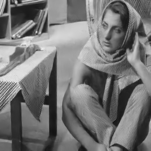 |
| clean image (Barbara) | BM3D: dB | MLP: dB |
 |
 |
 |
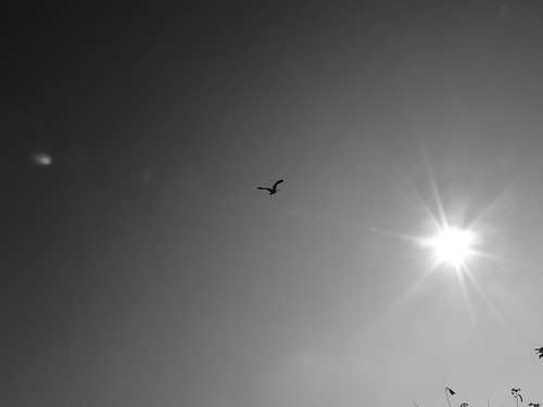
| clean image (004513) | BM3D: dB | MLP: dB |
 |
 |
 |
| clean image (198054) | BM3D: dB | MLP: dB |
5.1 Detailed comparison on one noise level
We will now compare the results achieved with an MLP to results achieved with other denoising algorithms on AWG noise with . We choose the MLP with architecture () because it delivered the best results. The MLP was trained for approximately backprops, see Burger et al. (2012b) for details.
Comparison on 11 standard test images:
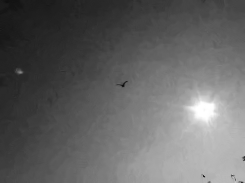
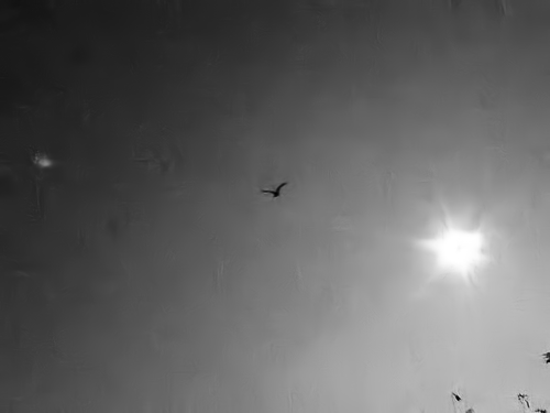
Table 1 summarizes the comparison of our approach (MLP) to the four other denoising algorithms. Our approach achieves the best result on of the test images and is the runner-up on one image. However, our method is clearly inferior to BM3D and NLSC on images “Barbara” and “House”. These two images contain a lot of regular structure (see Figure 3) and are therefore ideally suited for algorithms like BM3D and NLSC, which adapt to the noisy image. However, we outperform KSVD on both of these images even though KSVD is also an algorithm that is well-suited for these types of images. We also note that we outperform both KSVD and EPLL on every image.
 |
 |
| (a) | (b) |
Comparison on larger test sets
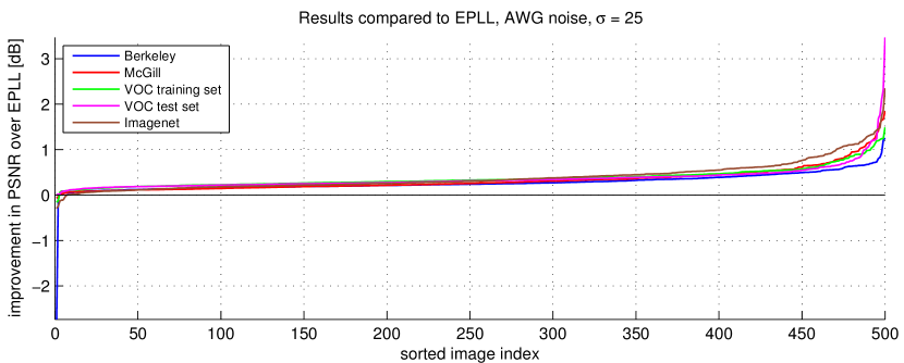
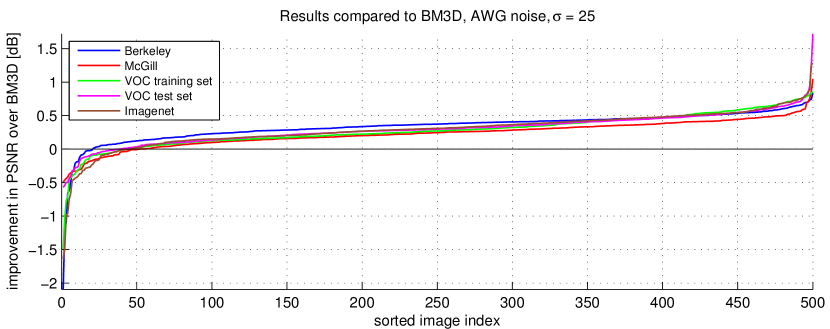
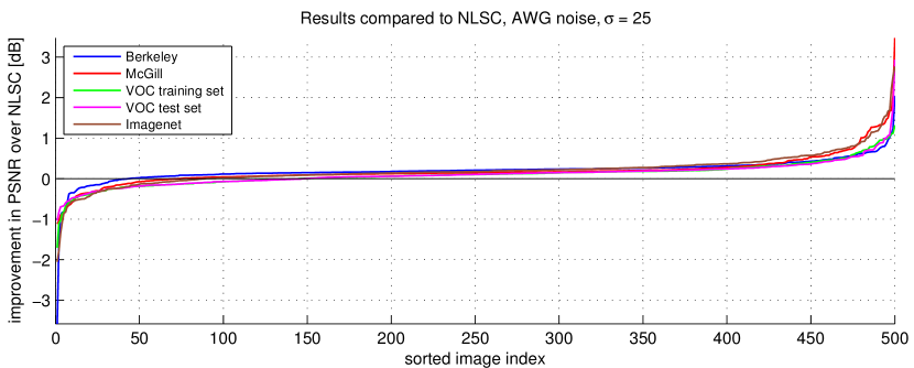
We now compare our approach to EPLL, BM3D and NLSC on the five larger test sets defined in section 4. Each dataset contains images, giving us a total of test images.
-
•
Comparison to EPLL: We outperform EPLL on () of the images, see Figure 5. The average improvement over all datasets is dB. On the VOC 2007 test set, we outperform EPLL on every image. The best average improvement over EPLL was on the subset of the ImageNet dataset (dB), whereas the smallest improvement was on the Berkeley dataset (dB). This is perhaps a reflection of the fact that EPLL was trained on a subset of the Berkeley dataset, whereas our approach was trained on the ImageNet dataset. For EPLL, the test set contains the training set. For our method, this is not the case, but it is plausible that the ImageNet dataset contains some form of regularity across the whole dataset.
-
•
Comparison to BM3D: We outperform BM3D on () of the images, see Figure 5. The average improvement over all datasets is dB. The largest average improvement was on the Berkeley dataset (dB), whereas the smallest average improvement was on the McGill dataset (dB).
-
•
Comparison to NLSC: We outperform NLSC on () of the images, see Figure 5. The average improvement over all datasets was dB. The largest average improvements were on the ImageNet subset and Berkeley dataset (dB), whereas the smallest average improvements were on the VOC 2011 training set and VOC 2007 test set (dB and dB respectively). This is perhaps a reflection of the fact that the initial dictionary of NLSC was trained on a subset of the VOC 2007 dataset (Mairal et al., 2010).
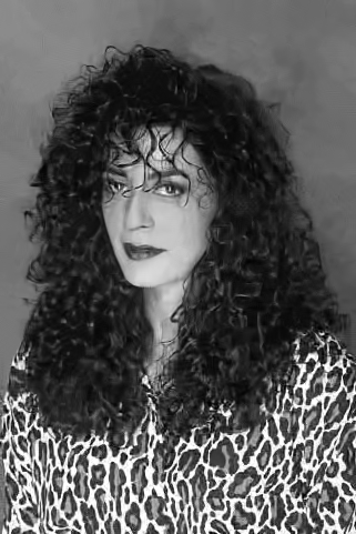
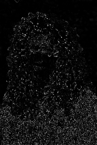
In summary, our method outperforms state-of-the-art denoising algorithms for AWG noise with . The improvement is consistent across datasets. We notice that our method tends to outperform BM3D on images with smooth areas such as the sky and on images which contain irregular structure, such as the hair of the woman in Figure 3. The fact that our method performs well on smooth surfaces can probably be explained by the fact that our method uses large input patches: This allows our method to handle low frequency noise. Methods using smaller patches (such as BM3D) are blind to lower frequencies. The fact that our method performs better than BM3D on images with irregular structures is explained by the block-matching approach employed by BM3D: The method cannot find similar patches in images with irregular textures.
5.2 Comparison on different noise variances
We have seen that our method achieves state-of-the-art results on AWG noise with . We now evaluate our approach on other noise levels. We use (low noise), (high noise), (very high noise) and (extremely high noise) for this purpose. We describe in Burger et al. (2012b) which architectures and patch sizes are used for the various noise levels.
| image | KSVD | EPLL | BM3D | NLSC | MLP |
|---|---|---|---|---|---|
| Barbara | 34.40dB | 33.59dB | 34.96dB | 34.96dB | 34.07dB |
| Boat | 33.65dB | 33.64dB | 33.89dB | 34.02dB | 33.85dB |
| C.man | 33.66dB | 33.99dB | 34.08dB | 34.15dB | 34.13dB |
| Couple | 33.51dB | 33.82dB | 34.02dB | 33.98dB | 33.89dB |
| F.print | 32.39dB | 32.12dB | 32.46dB | 32.57dB | 32.59dB |
| Hill | 33.37dB | 33.49dB | 33.60dB | 33.66dB | 33.59dB |
| House | 35.94dB | 35.74dB | 36.71dB | 36.90dB | 35.94dB |
| Lena | 35.46dB | 35.56dB | 35.92dB | 35.85dB | 35.88dB |
| Man | 33.53dB | 33.94dB | 33.97dB | 34.06dB | 34.10dB |
| Montage | 35.91dB | 36.45dB | 37.37dB | 37.24dB | 36.51dB |
| Peppers | 34.20dB | 34.54dB | 34.69dB | 34.78dB | 34.72dB |
| image | KSVD | EPLL | BM3D | NLSC | MLP |
|---|---|---|---|---|---|
| Barbara | 25.22dB | 24.83dB | 27.21dB | 27.13dB | 25.37dB |
| Boat | 25.90dB | 26.59dB | 26.72dB | 26.73dB | 27.02dB |
| C.man | 25.42dB | 26.05dB | 26.11dB | 26.36dB | 26.42dB |
| Couple | 25.40dB | 26.24dB | 26.43dB | 26.33dB | 26.71dB |
| F.print | 23.24dB | 23.59dB | 24.53dB | 24.25dB | 24.23dB |
| Hill | 26.14dB | 26.90dB | 27.14dB | 27.05dB | 27.32dB |
| House | 27.44dB | 28.77dB | 29.71dB | 29.88dB | 29.52dB |
| Lena | 27.43dB | 28.39dB | 28.99dB | 28.88dB | 29.34dB |
| Man | 25.83dB | 26.68dB | 26.76dB | 26.71dB | 27.08dB |
| Montage | 26.42dB | 27.13dB | 27.69dB | 28.02dB | 28.07dB |
| Peppers | 25.91dB | 26.64dB | 26.69dB | 26.73dB | 26.74dB |
| image | KSVD | EPLL | BM3D | NLSC | MLP |
|---|---|---|---|---|---|
| Barbara | 22.65dB | 22.95dB | 25.10dB | 25.03dB | 23.48dB |
| Boat | 23.59dB | 24.86dB | 25.04dB | 24.95dB | 25.43dB |
| C.man | 23.04dB | 24.19dB | 24.37dB | 24.24dB | 24.72dB |
| Couple | 23.43dB | 24.46dB | 24.71dB | 24.48dB | 25.09dB |
| F.print | 20.72dB | 21.44dB | 22.83dB | 22.48dB | 22.41dB |
| Hill | 24.21dB | 25.42dB | 25.60dB | 25.57dB | 25.97dB |
| House | 24.53dB | 26.69dB | 27.46dB | 27.64dB | 27.75dB |
| Lena | 24.87dB | 26.50dB | 27.16dB | 27.17dB | 27.66dB |
| Man | 23.76dB | 25.07dB | 25.29dB | 25.15dB | 25.63dB |
| Montage | 23.58dB | 24.86dB | 25.36dB | 25.20dB | 25.93dB |
| Peppers | 23.09dB | 24.52dB | 24.71dB | 24.46dB | 24.87dB |
| image | KSVD | EPLL | BM3D | NLSC | MLP |
|---|---|---|---|---|---|
| Barbara | 18.08dB | 20.79dB | 19.74dB | 20.99dB | 21.37dB |
| Boat | 18.42dB | 21.60dB | 20.49dB | 21.48dB | 22.47dB |
| C.man | 18.00dB | 20.48dB | 19.65dB | 20.50dB | 21.28dB |
| Couple | 18.26dB | 21.48dB | 20.39dB | 21.29dB | 22.16dB |
| F.print | 16.75dB | 17.06dB | 17.46dB | 18.51dB | 18.57dB |
| Hill | 18.69dB | 22.63dB | 20.98dB | 22.62dB | 23.33dB |
| House | 18.20dB | 22.52dB | 21.19dB | 21.95dB | 23.80dB |
| Lena | 18.68dB | 22.96dB | 21.38dB | 23.20dB | 24.24dB |
| Man | 18.49dB | 22.10dB | 20.59dB | 21.72dB | 22.85dB |
| Montage | 17.91dB | 20.48dB | 19.69dB | 20.40dB | 20.93dB |
| Peppers | 17.47dB | 20.26dB | 19.58dB | 19.53dB | 20.81dB |
Comparison on 11 standard test images:
Table 2 compares our method against KSVD, EPLL, BM3D and NLSC on the test set of standard test images for . Our method outperforms KSVD on ten images, EPLL on all images, BM3D on four images and NLSC on three images. Our method achieves the best result of all algorithms on two images. Like for , BM3D and NLSC perform particularly well for images “Barbara” and “House”.
Table 3 performs the same comparison for . Our method outperforms all others on of the images. BM3D and NLSC still perform significantly better on the image “Barbara”. We outperform KSVD and EPLL on every image.
For , our method outperforms all others on of the images, see Table 4. BM3D and NLSC still perform significantly better on the image “Barbara”.
For , our method outperforms all other methods on all images, see Table 5. It was suggested by Levin and Nadler (2011) that image priors are not useful at extremely high noise levels. However, our results suggest otherwise: Our method is the best-performing method on this noise level. The second best performing method, EPLL, is also a prior-based method. The improvement of our method over BM3D (which is not prior-based) is often very high (almost dB on image “Lena”).
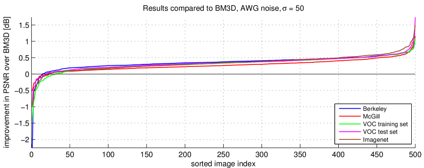
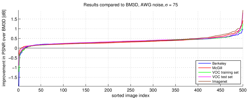
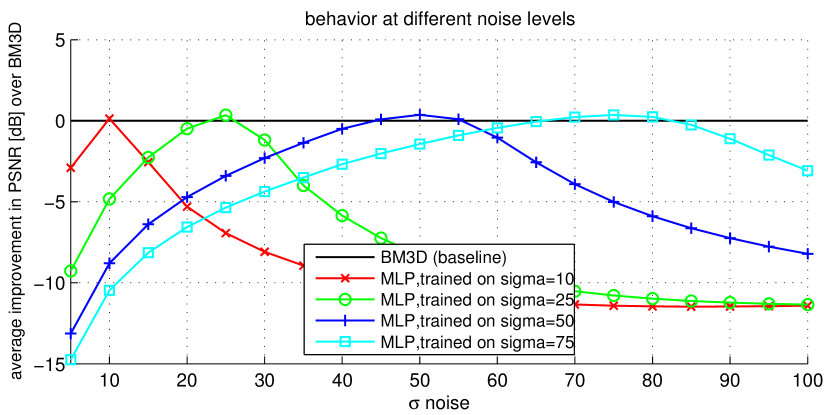
Comparison on 2500 test images:
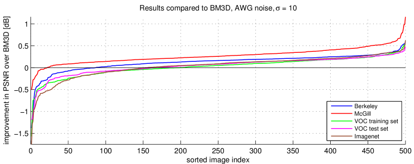
Figure 6 (top) compares the results achieved with an MLP on to BM3D. We outperform BM3D on () of the images. The average improvement over all images is dB. The largest average improvement is on the McGill dataset (dB), whereas the smallest average improvement is on the VOC training set (dB). The improvement in PSNR is very small on the VOC training set, but we observe an improvement on () of the images.
Figure 6 (middle) compares the results achieved with an MLP on to BM3D. We outperform BM3D on () of the images. The average improvement over all datasets is dB. The largest average improvement is on the Berkeley dataset (dB), whereas the smallest average improvement is on the McGill dataset (dB). This is an even greater improvement over BM3D than on , see Figure 5.
Figure 6 (bottom) compares the results achieved with an MLP on to BM3D. We outperform BM3D on () of the images. The average improvement over all datasets is dB. The average improvement is almost the same for all datasets, ranging from to dB.
Adaptation to other noise levels:
How do the MLPs perform on noise levels they have not been trained on? Figure 7 summarizes the results achieved by MLPs on noise levels they have not been trained on and compares these results to BM3D. The results are averaged over the images in the Berkeley dataset. We varied between and in steps of . We see that the MLPs achieve better results than BM3D on the noise levels they have been trained on. However, the performance degrades quickly for noise levels they have not been trained on. Exceptions are the MLPs trained on and , which also outperform BM3D on and (for the MLP trained on ) and and (for the MLP trained on ).
We conclude than our method is particularly well suited for medium to high noise levels. We outperform the previous state-of-the-art on all noise levels, but for , the improvement is rather small (dB). However, our method has to be trained on each noise level in order to achieve good results.
6 Results: Comparison with theoretical bounds
It has been observed that recent denoising algorithms tend to perform approximately equally well (Chatterjee and Milanfar, 2010), which naturally raises the question of whether recent state-of-the-art algorithms are close to an inherent limit on denoising quality. Two approaches to estimating bounds on denoising performance have been followed (Chatterjee and Milanfar, 2010; Levin and Nadler, 2011). We will relate the results obtained by our algorithm to these bounds.
 |
 |
6.1 Clustering-based bounds
The authors of (Chatterjee and Milanfar, 2010) derive bounds on image denoising capability. The authors make a “cluster” assumption about images: Each patch in a noisy image is assigned to one of a finite number of clusters. Clusters with more patches are denoised better than clusters with fewer patches. According to their bounds, improvements over existing denoising algorithms are mainly to be achieved on images with simple geometric structure (the authors use a synthetic “box” image as an example), whereas current denoising algorithms (and BM3D in particular) are already very close to the theoretical bounds for images with richer geometric structure.
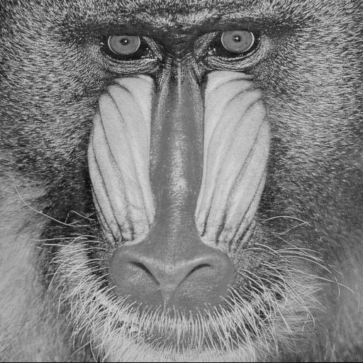
Figure 8 shows two images with richer structure and on which BM3D is very close to the estimated theoretical bounds for (Chatterjee and Milanfar, 2010, Fig. 11). Very little, if any, improvement is expected on these images. Yet, we outperform BM3D by dB and dB on these images, which is a significant improvement.
The MLP does not operate according to the cluster assumption (it operates on a single patch at a time) and it performs particularly well on images with rich geometric structure. We therefore speculate that the cluster assumption might not be a reasonable assumption to derive ultimate bounds on image denoising quality.
| worst | best | mean | |
| BLSGSM (Portilla et al., 2003) | 22.65dB | 23.57dB | 23.15dB |
| KSVD (Aharon et al., 2006) | 21.69dB | 22.59dB | 22.16dB |
| NLSC (Mairal et al., 2010) | 21.39dB | 22.49dB | 21.95dB |
| BM3D (Dabov et al., 2007) | 22.94dB | 23.96dB | 23.51dB |
| BM3D, step1 (Dabov et al., 2007) | 21.85dB | 22.79dB | 22.35dB |
| EPLL (Zoran and Weiss, 2011) | 22.94dB | 24.07dB | 23.56dB |
| MLP | 23.32dB | 24.34dB | 23.85dB |
 |
 |
| (a) Original image | (b) Noisy input, dB |
 |
 |
| (c) BM3D, dB | (d) MLP, dB |
6.2 Bayesian bounds
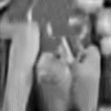
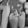
Levin and Nadler (2011) derive bounds on how well any denoising algorithm can perform. The bounds are dependent on the patch size, where larger patches lead to better results. For large patches and low noise, tight bounds cannot be estimated. On the image depicted in Figure 9a (a down-sampled and cropped version of the image “Peppers”) and for noise level , the theoretically best achievable result using patches of size is estimated to be dB better than BM3D (dB for BM3D and for the estimated bound).
We tested an MLP trained on as well as other methods (including BM3D) on the same image and summarize the results in Table 6. We used different noisy versions of the same clean image and report the worst, best and average results obtained. For BM3D, we obtain results that are in agreement with those obtained by Levin and Nadler (2011), though we note that the difference between the worst and best result is quite large: Approximately dB. The high variance in the results is due to the fact that the test image is relatively small and the noise variance quite high. The results obtained with BLSGSM and KSVD are also in agreement with those reported by Levin and Nadler (2011). NLSC achieves results that are much worse than those obtained by BM3D on this image and this noise level. EPLL achieves results that are on par with those achieved by BM3D.
BM3D achieves a mean PSNR of dB and our MLP achieves a mean PSNR of dB, an improvement of dB. Visually, the difference is noticeable, see Figure 9. This is a much greater improvement than was estimated to be possible by Levin and Nadler (2011), using patches of size . This is possible because of the fact that we used larger patches. Levin and Nadler (2011) were unable to estimate tight bounds for larger patch sizes because of their reduced density in the dataset of clean patches.
Levin and Nadler (2011) BM3D as a method that uses patches of size . However, BM3D is a two-step procedure. It is true that BM3D uses patches of size (for noise levels above ) in its first step. However, the second step of the procedure effectively increases the support size: In the second step, the patches “see beyond” what they would have seen in the first step, but it is difficult to say by how much the support size is increased by the second step. Therefore, a fairer comparison would have been to compare the estimated bounds against only the first step of BM3D. If only the first step of BM3D is used, the mean result is dB. Therefore, if the constraint on the patch sizes is strictly enforced for BM3D, the difference between the theoretically best achievable result and BM3D is larger than suggested by Levin and Nadler (2011).
6.3 Bayesian bounds with unlimited patch size
More recently, bounds on denoising quality achievable using any patch size have been suggested (Levin et al., 2012). This was done by extrapolating bounds similar to those suggested by Levin and Nadler (2011) to larger patch sizes (including patches of infinite size). For and , the bounds lie dB and dB above the results achieved by BM3D, respectively. The improvements of our approach over BM3D on these noise levels (estimated on images) are dB and dB, respectively. Our approach therefore reaches respectively and of the remaining possible improvement over BM3D. Furthermore, Levin et al. (2012) suggest that increasing the patch size suffers from a law of diminishing returns. This is particularly true for textured image content: The larger the patch size, the harder it becomes to find enough training data. Levin et al. (2012) therefore suggest that increasing the patch size should be the most useful for smooth image content. The observation that our method performs much better than BM3D on images with smooth areas (see middle row in Figure 3) is in agreement with this statement. The fact that image denoising is cursed with a law of diminishing returns also suggests that the remaining available improvement will be increasingly difficult to achieve. However, Levin et al. (2012) suggest that patch-based denoising can be improved mostly in flat areas and less in textures ones. Our observation that the MLP performs particularly well in areas with complicated structure (such as on the bottom image in Figure 3 or both images in Figure 8) shows that large improvements over BM3D on images with complicated textures are possible.
7 Results: comparison on non-AWG noise
Virtually all denoising algorithms assume the noise to be AWG. However, images are not always corrupted by AWG noise. Noise is not necessarily additive, white, Gaussian and signal independent. For instance in some situations, the imaging process is corrupted by Poisson noise (such as photon shot noise). Denoising algorithms which assume AWG noise might be applied to such images using some image transform (Mäkitalo and Foi, 2011). Rice-distributed noise, which occurs in magnetic resonance imaging, can be handled similarly (Foi, 2011).
 |
 |
 |
| “stripe” noise: dB | s p noise: dB | JPEG quantization: dB |
 |
 |
 |
| BM3D (Dabov et al., 2007): dB | median filtering: dB | SA-DCT (Foi et al., 2007): dB |
 |
 |
 |
| MLP: dB | MLP: dB | MLP:dB |
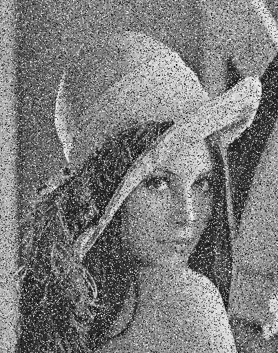
In most cases however, it is more difficult or even impossible to find Gaussianizing transforms. In such cases, a possible solution is to create a denoising algorithm specifically designed for that noise type. MLPs allow us to effectively learn a denoising algorithm for a given noise type, provided that noise can be simulated. In the following, we present results on three noise types that are different from AWG noise. We make no effort to adapt our architecture or procedure in general to the specific noise type but rather use an architecture that yielded good results for AWG noise (four hidden layers of size and input and output patches of size ).
7.1 Stripe noise
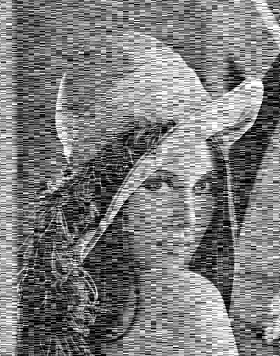
It is often assumed that image data contains structure, whereas the noise is uncorrelated and therefore unstructured. In cases where the noise also exhibits structure, this assumption is violated and denoising results become poor. We here show an example where the noise is additive and Gaussian (with ), but where horizontally adjacent noise values have the same value.
Since there is no canonical denoising algorithm for this noise, we choose BM3D as the competitor. An MLP trained on 82 million training examples outperforms BM3D for this type of noise, see left column of Figure 10.
7.2 Salt and pepper noise
When the noise is additive Gaussian, the noisy image value is still correlated to the original image value. With salt and pepper noise, noisy values are not correlated with the original image data. Each pixel has a probability of being corrupted. A corrupted pixel has probability of being set to ; otherwise, it is set to highest possible value ( for -bit images). We show results with .
A common algorithm for removing salt and pepper noise is median filtering. We achieved the best results with a filter size of and symmetrically extended image boundaries. We also experimented with BM3D (by varying the value of ) and achieved a PSNR of dB. An MLP trained on 88 million training examples outperforms both methods, see middle column of Figure 10.
The problem of removing salt and pepper noise is reminiscent of the in-painting problem, except that it is not known which pixels are to be in-painted. If one assumes that the positions of the corrupted pixels are known, the pixel values of the non-corruped pixels can be copied from the noisy image, since these are identical to the ground truth values. Using this assumption, we achieve dB with median filtering and dB with the MLP.
7.3 JPEG quantization artifacts
Such artifacts occur due to the JPEG image compression algorithm. The quantization process removes information, therefore introducing noise. Characteristics of JPEG noise are blocky images and loss of edge clarity. This kind of noise is not random, but rather completely determined by the input image. In our experiments we use JPEG’s quality setting , creating visible artifacts.
A common method to enhance JPEG-compressed images is to shift the images, re-apply JPEG compression, shift back and average (Nosratinia, 2001). This method achieves a PSNR of dB on our image. We also compare against the state-of-the-art in JPEG de-blocking (Foi et al., 2007).
An MLP trained on 58 million training examples with that noise outperforms both methods, see right column of Figure 10. In fact, the method described by Nosratinia (2001) achieves an improvement of only dB over the noisy image, whereas our method achieves an improvement of dB. SA-DCT (Foi et al., 2007) achieves an improvement of dB.
 |
 |
| noisy, peak=1, PSNR: dB | noisy, peak=20, PSNR: dB |
 |
 |
| GAT+BM3D (Mäkitalo and Foi, 2012a) | GAT+BM3D (Mäkitalo and Foi, 2012a) |
| PSNR: dB | PSNR: dB |
 |
 |
| MLP: dB | MLP: dB |
7.4 Mixed Poisson-Gaussian noise
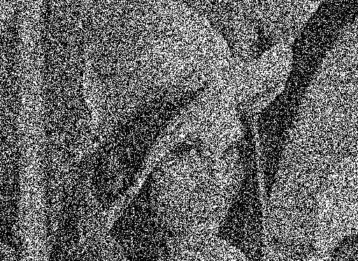
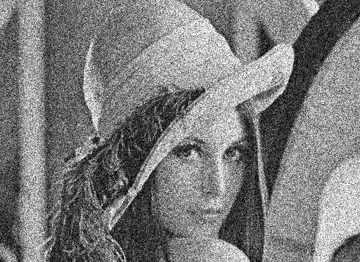
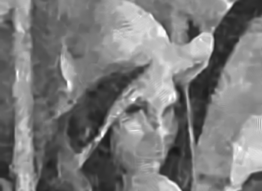
In photon-limited imaging, observations are usually corrupted by mixed Poisson-Gaussian noise (Mäkitalo and Foi, 2012a; Luisier et al., 2011). Observations are assumed to come from the following model:
| (3) |
where is Poisson-distributed with mean and is Gaussian-distributed with mean and variance . One can regard to be the underlying “true” image of which one wishes to make a noise-free observation. To generate a noisy image from a clean one, we follow the setup used by by Mäkitalo and Foi (2012a) and Luisier et al. (2011): We take the clean image and scale it to a given peak value, giving us . Applying (3) gives us a noisy image .
Two canonical approaches exist for denoising in the photon-limited setting: (i) Applying a variance stabilizing transform on the noisy image, running a denoising algorithm designed for AWG noise (such as BM3D) on the result and finally applying the inverse of the variance stabilizing transform, and (ii) designing a denoising algorithm specifically for mixed Poisson-Gaussian noise. GAT+BM3D (Mäkitalo and Foi, 2012a) is an example of the first approach, whereas UWT/BDCT PURE-LET (Luisier et al., 2011) is an example of the second approach. In the case where a variance-stabilizing transform such as the Anscombe transformation or the generalized Anscombe transformatoin (GAT) (Starck et al., 1998) is applied, the difficulty lies in the design of the inverse transform (Mäkitalo and Foi, 2009, 2011a, 2011b, 2012b). Designing a denoising algorithm specifically for Poisson-Gaussian noise is also a difficult task, but can potentially lead to better results.
| image | peak | GAT+BM3D | UWT/BDCT (Foi) | UWT/BDCT (Luisier) | MLP |
|---|---|---|---|---|---|
| Barbara | 1 | 20.83dB | - | 20.79dB | 21.44dB |
| Barbara | 20 | 27.52dB | - | 27.33dB | 26.08dB |
| Cameraman | 1 | 20.34dB | 20.35dB | 20.48dB | 21.66dB |
| Cameraman | 20 | 26.83dB | 25.92dB | 26.93dB | 26.93dB |
| Lena | 1 | 22.96dB | 22.83dB | - | 24.26dB |
| Lena | 20 | 29.39dB | 28.46dB | - | 29.89dB |
| Fluo.cells | 1 | 24.54dB | 25.13dB | 25.25dB | 25.56dB |
| Fluo.cells | 20 | 29.66dB | 29.47dB | 31.00dB | 29.98dB |
| Moon | 1 | 22.84dB | - | 23.49dB | 23.48dB |
| Moon | 20 | 25.28dB | - | 26.33dB | 25.71dB |
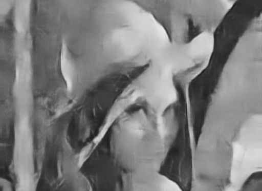
Our approach to denoising photon-limited data is to train an MLP on data corrupted with mixed Poisson-Gaussian noise. We trained an MLP on noisy images using a peak value of and another MLP for peak value , both on million examples. For the Gaussian noise, we set to the peak value divided by , again following the setup used by Mäkitalo and Foi (2012a) and Luisier et al. (2011). We compare our results against GAT+BM3D (Mäkitalo and Foi, 2012a), which is considered state-of-the-art. We compare on further images in Table 7. For UWT/BDCT PURE-LET (Luisier et al., 2011), we noticed a discrepancy between the results reported by Mäkitalo and Foi (2012a) and by Luisier et al. (2011) and therefore report both. We see that the MLPs outperform the state-of-the art on image “Lena” in both settings.
 |
 |
| (a) | (b) |
8 Combining BM3D and MLPs: block-matching MLPs
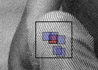
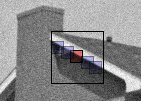
Many recent denoising algorithms rely on a block-matching procedure. This most notably includes BM3D (Dabov et al., 2007), but also NLSC (Mairal et al., 2010). The idea is to find patches similar to a reference patch and to exploit these “neighbor” patches for better denoising. More precisely, the procedure exploits the fact that the noise in the different patches is independent, whereas the (clean) image content is correlated. Figure 12 shows the effect of the procedure on two images.
Since this technique has been used with so much success, we ask the question: Can MLPs be combined with a block matching procedure to achieve better results? In particular, can we achieve better results on images where we perform rather poorly compared to BM3D and NLSC, namely images with repeating structure? To answer this question, we train MLPs that take as input not only the reference patch, but also its nearest neighbors in terms of distance. We will see that such block-matching MLPs can indeed achieve better on images with repeating structure. However, they also sometimes achieve worse results than plain MLPs and do not achieve better results on average.
8.1 Differences to previous MLPs
Previously, we trained MLPs to take as input one noisy image patch and to output one denoised image patch. The best results were achieved when the input patch size was and the output patch was of size . Now, we train MLPs to take as input noisy patches of size or and to output one noisy patch of the same size. The block matching procedure has to be performed for each training pair, slowing down the training procedure by approximately a factor of . One could also imagine MLPs taking as input patches and providing patches as output, but we have been less successful with that approach. In all our experiments, we used . The architecture of the MLP we used had four hidden layers; the first hidden layer was of size and the remaining three were of size . We discuss the training procedure in Burger et al. (2012b).
We note that our block-matching procedure is different from the one employed by BM3D in a number of ways: (i) We always use the same number of neighbors, whereas BM3D chooses all patches whose distance to the reference patch is smaller than a given threshold, up to a maximum of neighbors, (ii) BM3D is a two-step approach, where the denoising result of the first step is merely used to find better neighbors in the second step. We find neighbors directly in the noisy image. (iii) When the noise level is higher than , BM3D employs “coarse pre-filtering” in the first step: patches are first transformed (using a 2D wavelet or DCT transform) and then hard-thresholded. This is already a form of denoising and helps to find better neighbors. We employ no such strategy. (iv) BM3D has a number of hyper-parameters (patch and stride sizes, type of 2D transform, thresholding and matching coefficients). The value of the hyper-parameters are different for the two steps of the procedure. We have fewer hyper-parameters, in part due to the fact that our procedure consists of a single step. We also choose to set the search stride size to the canonical choice of .
8.2 Block-matching MLPs vs. plain MLPs
Results on 11 standard test images:
Table 8 summarizes the results achieved by an MLP using block matching with , patches of size and . We omit KSVD and EPLL from the comparison because the block-matching MLP and the plain MLP both outperform the two algorithms on every image. The mean result achieved on the images is dB higher for the block-matching MLP than for the plain MLP. The block-matching MLP outperforms NLSC on images, whereas the plain MLP outperforms NLSC on images. The block-matching MLP outperforms the plain MLP on images. The improvement on the plain MLP is the largest on images Barbara, House and Peppers (approximately dB on each). The largest decrease in performance compared to the plain MLP is observed on image Lena (a decrease of dB). We see that the block-matching procedure is most useful on images with repeating structure, as found in the images “Barbara” and “House”. However, both BM3D and NLSC achieve results that are far superior to the block-matching MLP on image “Barbara”.
| image | BM3D | NLSC | MLP | BM-MLP |
|---|---|---|---|---|
| Barbara | 30.67dB | 30.50dB | 29.52dB | 29.75dB |
| Boat | 29.86dB | 29.86dB | 29.95dB | 29.92dB |
| C.man | 29.40dB | 29.46dB | 29.60dB | 29.67dB |
| Couple | 29.68dB | 29.63dB | 29.75dB | 29.73dB |
| F.print | 27.72dB | 27.63dB | 27.67dB | 27.63dB |
| Hill | 29.81dB | 29.80dB | 29.84dB | 29.87dB |
| House | 32.92dB | 33.08dB | 32.52dB | 32.75dB |
| Lena | 32.04dB | 31.87dB | 32.28dB | 32.17dB |
| Man | 29.58dB | 29.62dB | 29.85dB | 29.86dB |
| Montage | 32.24dB | 32.15dB | 31.97dB | 32.11dB |
| Peppers | 30.18dB | 30.27dB | 30.27dB | 30.53dB |
Results on larger test sets:
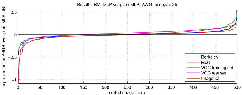
The block-matching MLP outperforms the plain MLP on () of the images, see Figure 13. The average improvement over all datasets is dB. The largest improvement was on the VOC training set (dB). On the McGill dataset, the block-matching MLP was worse by dB. The block-matching MLP and the plain MLP therefore achieve approximately equal results on average.
 |
 |
| (a) | (b) |
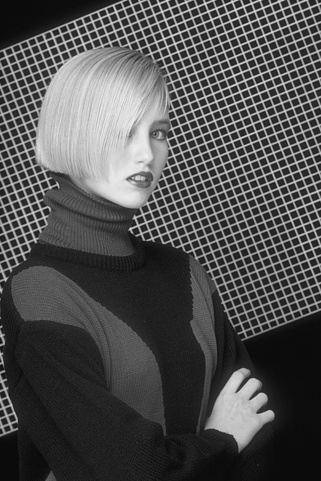
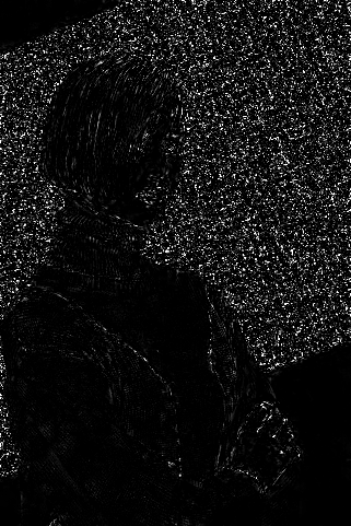
On image in the Berkeley dataset, the MLP with block-matching outperforms the plain MLP by dB. This is an image similar to the “Barbara” images in that it contains a lot of regular structure, see Figure 14.
On image in the VOC test set, see Figure 3, the MLP with block-matching performs dB worse than the plain MLP. This can be explained by the fact that the block-matching MLP uses smaller patches, making it blind to low frequency noise, resulting in a decrease in performance on images with smooth surfaces.
Conclusion:
On average, the results achieved with a block-matching MLP are almost equal to those achieved by a plain MLP. Plain MLPs perform better on images with smooth surfaces whereas the block-matching MLPs provide better results on images with repeating structure. However, combining MLPs with the block-matching procedure did not allow us to outperform BM3D and NLSC on image “Barbara”. We emphasize that the block-matching MLPs use less information as input than the plain MLPs, yet still achieve results that are comparable on average. Block-matching is a search procedure and therefore cannot be learned by a feed-forward architecture with few layers.
9 Code
We make available a Matlab toolbox allowing to denoise images with our trained MLPs on CPU at http://people.tuebingen.mpg.de/burger/neural_denoising/. The script demo.m loads the image “Lena”, adds AWG noise with on the image and denoises with an MLP trained on the same noise level. Running the script produces an output similar to the following
>> demo Starting to denoise... Done! Loading the weights and denoising took 121.4 seconds PSNRs: noisy: 20.16dB, denoised: 32.26dB
and display the clean, noisy and denoised images. Denoising an image is performed using the function fdenoiseNeural:
>> im_denoised = fdenoiseNeural(im_noisy, noise_level, model);
The function takes as input a noisy image, the level of noise and a struct containing the step size and the width of the Gaussian window applied on denoised patches.
>> model = {};
>> model.step = 3;
>> model.weightsSig = 2;
10 Discussion and Conclusion
In this paper, we have described a learning-based approach to image denoising. We have compared the results achieved by our approach against other algorithms and against denoising bounds, allowing us to draw a number of conclusions.
Comparison against state-of-the-art algorithms:
-
•
KSVD: We compared our method against KSVD (Elad and Aharon, 2006) on test images and for all noise levels. KSVD outperforms our method only on image Barbara with .
-
•
EPLL: We outperform EPLL (Zoran and Weiss, 2011) on more than of the test images on , and by dB on average. For all other noise levels and test images, we always outperform EPLL.
-
•
NLSC: We outperform NLSC (Mairal et al., 2010) more approximately of the test images on , and by dB on average. The higher the noise level, the more favorably we perform against NLSC. NLSC has an advantage over our method on images with repeating structure, such as Barbara and House. However, at high noise levels, this advantage disappears.
-
•
BM3D: We outperform BM3D Dabov et al. (2007) on approximately of the test images on , and by dB on average. Otherwise, the same conclusions as for NLSC hold: The higher the noise level, the more favorably we perform against BM3D. BM3D has an advantage over our method on images with repeating structure, such as Barbara and House. However, at high noise levels, this advantage disappears.
Our method compares the least favorably compared to other methods on the lowest noise level (), but we still achieve an improvement of dB over BM3D on that noise level.
Comparison against denoising bounds:
-
•
Clustering-based bounds Our results exceed the bounds estimated by Chatterjee and Milanfar (2010). This is possible because we violate the “patch cluster” assumption made by the authors. In addition, Chatterjee and Milanfar (2010) suggest that there is almost no room for improvement over BM3D on images with complex textures. We have seen that is not the case: Our approach is often significantly better than BM3D on images with complex textures.
-
•
Bayesian patch-based bounds Levin and Nadler (2011) estimate denoising bounds in a Bayesian setting, for a given patch size. Our results are superior to these bounds This is possible because we use larger patches than is assumed by Levin and Nadler (2011). The same authors also suggest that image priors should be the most useful for denoising at medium noise levels, but not so much at high noise levels. Yet, our method achieves the greatest improvements over other methods at high noise levels.
Similar bounds estimated for patches of infinite size are estimated by Levin et al. (2012). We make important progress toward reaching these bounds: Our approach reaches almost half the theoretically possible gain over BM3D. Levin et al. (2012) agree with Chatterjee and Milanfar (2010) that there is little room for improvement on patches with complex textures. We have seen that this is not the case.
Comparison on other noise types:
We have seen that our method can be adapted to other types of noise by merely switching the training data. We have shown that we achieve good results are on stripe noise, salt-and-pepper noise, JPEG quantization artifacts and mixed Poisson-Gaussian noise. In the latter two cases we seem to be competitive with the state-of-the-art.
Block-matching MLPs:
We have also seen that results can sometimes be improved a little further using a block-matching procedure. However, this comes at the cost of a more complicated training procedure and longer training and test times. In addition, the block-matching procedure is highly task-specific: It has been shown to work well on AWG noise, but it is not clear that it is useful for all kinds of noise. In addition, plain MLPs could potentially be used for other low-level vision tasks. It is not clear that the block-matching procedure is useful for other tasks. We here face an often encountered conundrum: Is it worth exploiting task-specific knowledge? This often leads to better results, at the cost of more engineering.
Computation time:
Denoising an image using an MLP takes approximately a minute on CPU and less than seconds on GPU. This is not as fast as BM3D, but much faster than approaches that require learning a dictionary, such as KSVD or NLSC which can take almost an hour per image (on CPU).
Training procedure:
Part 2 of this paper (Burger et al., 2012b), describes our training procedure in detail and shows the importance of various factors influencing the quality of the results, such as the size of the training corpus, the architecture of the multi-layer perceptrons and the size of the input and output patches. We show that some setups lead to surprisingly bad results and provide an explanation for the phenomena.
Understanding denoising:
Also not discussed in this paper is the operating principle of the multi-layer perceptrons: How do they achieve denoising? Trained neural networks are often seen as “black boxes”, but we will see in Burger et al. (2012b) that in this case, the behavior can be understood, at least to some extent.
Outlook:
On some images, our method outperforms BM3D by more than dB and NLSC by more than dB, see Section 5. Our method therefore seems to have a clear advantage over other methods on some images. However, we have seen that our approach sometimes achieves results that are much worse than the previous state-of-the-art. This happens especially on images with a lot of regular structure, such as the image “Barbara”. Our attempt to ameliorate the situation using a block-matching procedure was only partially successful. A question therefore begs to be asked: Can we find an approach that achieves state-of-the-art results on every image? An approach combining several algorithms, such as the one proposed by Jancsary et al. (2012) might be able to solve that problem.
References
- Aharon et al. (2006) M. Aharon, M. Elad, and A. Bruckstein. K-svd: An algorithm for designing overcomplete dictionaries for sparse representation. IEEE Transactions on Signal Processing (TIP), 54(11):4311–4322, 2006.
- Bengio (2009) Y. Bengio. Learning deep architectures for ai. Foundations and Trends in Machine Learning, 2(1):1–127, 2009.
- Bengio and Glorot (2010) Yoshua Bengio and Xavier Glorot. Understanding the difficulty of training deep feedforward neural networks. In Proceedings of AISTATS, volume 9, pages 249–256, 2010.
- Buades et al. (2005) A. Buades, C. Coll, and J.M. Morel. A review of image denoising algorithms, with a new one. Multiscale Modeling and Simulation, 4(2):490–530, 2005.
- Burger et al. (2012a) H.C. Burger, C.J. Schuler, and S. Harmeling. Image denoising: Can plain neural networks compete with bm3d? IEEE Conference on Computer Vision and Pattern Recognition (CVPR), pages 2392–2399, 2012a.
- Burger et al. (2012b) H.C. Burger, C.J. Schuler, and S. Harmeling. Image denoising with multi-layer perceptrons, part 2: training trade-offs and analysis of hidden activation patterns. Submitted to the Journal of Machine Learning Research (JMLR), 2012b.
- Chang et al. (2002) S.G. Chang, B. Yu, and M. Vetterli. Adaptive wavelet thresholding for image denoising and compression. IEEE Transactions on Image Processing (TIP), 9(9):1532–1546, 2002.
- Chatterjee and Milanfar (2010) P. Chatterjee and P. Milanfar. Is denoising dead? IEEE Transactions on Image Processing (TIP), 19(4):895–911, 2010.
- Cybenko (1989) G. Cybenko. Approximation by superpositions of a sigmoidal function. Mathematics of Control, Signals, and Systems (MCSS), 2(4):303–314, 1989.
- Dabov et al. (2007) K. Dabov, A. Foi, V. Katkovnik, and K. Egiazarian. Image denoising by sparse 3-D transform-domain collaborative filtering. IEEE Transactions on Image Processing (TIP), 16(8):2080–2095, 2007.
- Deng et al. (2009) J. Deng, W. Dong, R. Socher, L.J. Li, K. Li, and L. Fei-Fei. Imagenet: A large-scale hierarchical image database. In IEEE Conference on Computer Vision and Pattern Recognition (CVPR), pages 248–255. IEEE, 2009.
- Elad and Aharon (2006) M. Elad and M. Aharon. Image denoising via sparse and redundant representations over learned dictionaries. IEEE Transactions on Image Processing (TIP), 15(12):3736–3745, 2006.
- Estrada et al. (2009) F. Estrada, D. Fleet, and A. Jepson. Stochastic image denoising. In British Machine Vision Conference (BMVC), 2009.
- Everingham et al. (2007) M. Everingham, L. Van Gool, C. K. I. Williams, J. Winn, and A. Zisserman. The PASCAL Visual Object Classes Challenge 2007 (VOC2007) Results. http://www.pascal-network.org/challenges/VOC/voc2007/workshop/index.html, 2007.
- Foi (2011) A. Foi. Noise estimation and removal in mr imaging: The variance-stabilization approach. In IEEE International Symposium on Biomedical Imaging: From Nano to Macro, pages 1809–1814, 2011.
- Foi et al. (2007) A. Foi, V. Katkovnik, and K. Egiazarian. Pointwise shape-adaptive dct for high-quality denoising and deblocking of grayscale and color images. IEEE Transcations on Image Processing (TIP), 16(5):1395–1411, 2007.
- Funahashi (1989) K.I. Funahashi. On the approximate realization of continuous mappings by neural networks. Neural networks, 2(3):183–192, 1989.
- Gudbjartsson and Patz (1995) H. Gudbjartsson and S. Patz. The rician distribution of noisy mri data. Magnetic Resonance in Medicine, 34(6):910, 1995.
- Håstad and Goldmann (1991) J. Håstad and M. Goldmann. On the power of small-depth threshold circuits. Computational Complexity, 1(2):113–129, 1991.
- Hinton et al. (2006) G.E. Hinton, S. Osindero, and Y.W. Teh. A fast learning algorithm for deep belief nets. Neural Computation, 18(7):1527–1554, 2006.
- Hornik et al. (1989) K. Hornik, M. Stinchcombe, and H. White. Multilayer feedforward networks are universal approximators. Neural Networks, 2(5):359–366, 1989.
- Jain and Seung (2008) V. Jain and H.S. Seung. Natural image denoising with convolutional networks. Advances in Neural Information Processing Systems (NIPS), 21:769–776, 2008.
- Jancsary et al. (2012) J. Jancsary, S. Nowozin, and C. Rother. Loss-specific training of non-parametric image restoration models: A new state of the art. In European Conference of Computer Vision (ECCV). IEEE, 2012.
- Le Roux and Bengio (2010) N. Le Roux and Y. Bengio. Deep belief networks are compact universal approximators. Neural computation, 22(8):2192–2207, 2010.
- LeCun et al. (1998a) Y. LeCun, L. Bottou, Y. Bengio, and Haffner P. Gradient-based learning applied to document recognition. Proceedings of IEEE, 86(11):2278–2324, 1998a. URL http://leon.bottou.org/papers/lecun-98h.
- LeCun et al. (1998b) Y. LeCun, L. Bottou, G. Orr, and K. Müller. Efficient backprop. In Neural Networks, Tricks of the Trade, Lecture Notes in Computer Science LNCS 1524. Springer Verlag, 1998b. URL http://leon.bottou.org/papers/lecun-98x.
- Leshno et al. (1993) M. Leshno, V.Y. Lin, A. Pinkus, and S. Schocken. Multilayer feedforward networks with a nonpolynomial activation function can approximate any function. Neural networks, 6(6):861–867, 1993.
- Levin and Nadler (2011) A. Levin and B. Nadler. Natural Image Denoising: Optimality and Inherent Bounds. In IEEE Conference on Computer Vision and Pattern Recognition (CVPR), 2011.
- Levin et al. (2012) A. Levin, B. Nadler, F. Durand, and W.T. Freeman. Patch complexity, finite pixel correlations and optimal denoising. In European Conference on Computer Vision (ECCV), 2012.
- Luisier et al. (2011) F. Luisier, T. Blu, and M. Unser. Image denoising in mixed poisson–gaussian noise. IEEE Transactions on Image Processing (TIP), 20(3):696–708, 2011.
- Mairal et al. (2008) J. Mairal, M. Elad, G. Sapiro, et al. Sparse representation for color image restoration. IEEE Transactions on Image Processing (TIP), 17(1):53, 2008.
- Mairal et al. (2010) J. Mairal, F. Bach, J. Ponce, G. Sapiro, and A. Zisserman. Non-local sparse models for image restoration. In IEEE International Conference on Computer Vision (ICCV), pages 2272–2279, 2010.
- Mäkitalo and Foi (2009) M. Mäkitalo and A. Foi. On the inversion of the anscombe transformation in low-count poisson image denoising. In International Workshop on Local and Non-Local Approximation in Image Processing (LNLA), pages 26–32. IEEE, 2009.
- Mäkitalo and Foi (2011a) M. Mäkitalo and A. Foi. A closed-form approximation of the exact unbiased inverse of the anscombe variance-stabilizing transformation. IEEE Transactions on Image Processing (TIP), 20(9):2697–2698, 2011a.
- Mäkitalo and Foi (2011b) M. Mäkitalo and A. Foi. Optimal inversion of the anscombe transformation in low-count poisson image denoising. IEEE Transactions on Image Processing, 20(1):99–109, 2011b.
- Mäkitalo and Foi (2011) M. Mäkitalo and A. Foi. Optimal inversion of the anscombe transformation in low-count poisson image denoising. IEEE Transactions on Image Processing (TIP), 20:99–109, 2011.
- Mäkitalo and Foi (2012a) M. Mäkitalo and A. Foi. Optimal inversion of the generalized anscombe transformation for poisson-gaussian noise. IEEE Transactions on Image Processing (TIP), 2012a.
- Mäkitalo and Foi (2012b) M. Mäkitalo and A. Foi. Poisson-gaussian denoising using the exact unbiased inverse of the generalized anscombe transformation. In International Conference on Acoustics, Speech and Signal Processing (ICASSP), pages 1081–1084. IEEE, 2012b.
- Nosratinia (2001) A. Nosratinia. Enhancement of jpeg-compressed images by re-application of jpeg. The Journal of VLSI Signal Processing, 27(1):69–79, 2001.
- Olmos et al. (2004) A. Olmos et al. A biologically inspired algorithm for the recovery of shading and reflectance images. Perception, 33(12):1463, 2004.
- Pizurica et al. (2002) A. Pizurica, W. Philips, I. Lemahieu, and M. Acheroy. A joint inter- and intrascale statistical model for Bayesian wavelet based image denoising. IEEE Transactions on Image Processing (TIP), 11(5):545–557, 2002.
- Portilla et al. (2003) J. Portilla, V. Strela, M.J. Wainwright, and E.P. Simoncelli. Image denoising using scale mixtures of Gaussians in the wavelet domain. IEEE Transactions on Image Processing (TIP), 12(11):1338–1351, 2003.
- Ranzato et al. (2007) Marc’Aurelio Ranzato, Y-Lan Boureau, Sumit Chopra, and Yann LeCun. A unified energy-based framework for unsupervised learning. In Proc. Conference on AI and Statistics (AI-Stats), 2007.
- Roth and Black (2009) S. Roth and M.J. Black. Fields of experts. International Journal of Computer Vision (IJCV), 82(2):205–229, 2009. ISSN 0920-5691.
- Rudin et al. (1992) L.I. Rudin, S. Osher, and E. Fatemi. Nonlinear total variation based noise removal algorithms. Physica D: Nonlinear Phenomena, 60(1-4):259–268, 1992.
- Rumelhart et al. (1986) D.E. Rumelhart, G.E. Hinton, and R.J. Williams. Learning representations by back-propagating errors. Nature, 323(6088):533–536, 1986.
- Sermanet and LeCun (2011) P. Sermanet and Y. LeCun. Traffic Sign Recognition with Multi-Scale Convolutional Networks. In Proceedings of International Joint Conference on Neural Networks (IJCNN), 2011.
- Simoncelli and Adelson (1996) E.P. Simoncelli and E.H. Adelson. Noise removal via Bayesian wavelet coring. In Proceedings of the International Conference on Image Processing (ICIP), pages 379–382, 1996.
- Starck et al. (1998) J.L. Starck, F.D. Murtagh, and A. Bijaoui. Image processing and data analysis. Image Processing and Data Analysis, by Jean-Luc Starck and Fionn D. Murtagh and Albert Bijaoui, ISBN 0521599148. Cambridge, UK: Cambridge University Press, 1998.
- Tomasi and Manduchi (1998) C. Tomasi and R. Manduchi. Bilateral filtering for gray and color images. In Proceedings of the Sixth International Conference on Computer Vision (ICCV), pages 839–846, 1998.
- Vincent et al. (2010) P. Vincent, H. Larochelle, I. Lajoie, Y. Bengio, and P.A. Manzagol. Stacked denoising autoencoders: Learning useful representations in a deep network with a local denoising criterion. The Journal of Machine Learning Research (JMLR), 11:3371–3408, 2010.
- Weickert (1998) J. Weickert. Anisotropic diffusion in image processing. ECMI Series, Teubner-Verlag, Stuttgart, Germany, 1998.
- Weiss and Freeman (2007) Y. Weiss and W.T. Freeman. What makes a good model of natural images? In Proceedings of the IEEE Conference on Computer Vision and Pattern Recognition (CVPR), pages 1–8, 2007.
- Zhang and Salari (2005) S. Zhang and E. Salari. Image denoising using a neural network based non-linear filter in wavelet domain. In IEEE International Conference on Acoustics, Speech, and Signal Processing (ICASSP), volume 2, pages ii–989, 2005.
- Zoran and Weiss (2011) D. Zoran and Y. Weiss. From learning models of natural image patches to whole image restoration. In International Conference on Computer Vision (ICCV), pages 479–486. IEEE, 2011.