Exceptional points and quantum correlations in precise measurements

Abstract

We examine the physical manifestations of exceptional points and passage times in a two-level system which is subjected to quantum measurements and which admits a non-Hermitian description. Using an effective Hamiltonian acting in the two-dimensional space spanned by the evolving initial and final states, the effects of highly precise quantum measurements in which the monitoring device interferes significantly with the evolution dynamics of the monitored two-level system is analysed. The dynamics of a multipartite system consisting of the two-level system, a source of external potential and the measurement device is examined using correlation measures such as entanglement and non-classical quantum correlations. Results show that the quantum correlations between the monitored (monitoring) systems is considerably decreased (increased) as the measurement precision nears the exceptional point, at which the passage time is half of the measurement duration. The results indicate that the underlying mechanism by which the non-classical correlations of quantum systems are transferred from one subsystem to another may be better revealed via use of geometric approaches.

1 Introduction

Non-Hermitian systems [1, 2, 3, 4, 5, 6, 7, 8, 9, 10] play important roles in the dynamics of open quantum systems, and the appearance of non-Hermitian terms have profound implications for various physical, chemical and biological systems [10, 11, 12, 13, 14, 15, 16, 17, 18, 19, 20]. The striking difference between non-Hermitian physics and Hermitian physics lies in the occurrence of degeneracies such as exceptional points. This is the case even in situations where the non-Hermitian system is almost similar to its Hermitian counterpart.

The exceptional point is a topological defect which occurs when two eigenvalues of an operator coalesce as a result of a change in selected system parameters, with the two mutually orthogonal states merging into one self-orthogonal state, resulting in a singularity in the spectrum [21]. The critical parameter values at which the singularity appear are called exceptional points. These points are known to be located in the vicinity of a level repulsion [21] and unlike degenerate points, only one eigenfunction exists at the exceptional point due to the merging of two eigenvalues. This implies that the branch point at which the exceptional point forms is no longer single valued. The Berry phase around the exceptional point is generally treated using conventional techniques [22] which involves tracking a closed path in the Riemann space, however the procedure here involves transversing the loop twice since the eigenstates swaps positions after the first loop. From a quantum information perspective, the emergence of the exceptional point can be seen as a loss in information due to the decrease of eigenvalues in the parameter space, and it would be worthwhile to examine whether such a loss is counteracted by changes in another measurement subspace. In a recent work, we identified the critical temperatures at which exceptional points occurs in photosynthetic systems [20]. The experimental detection of the exceptional points remains a challenge, even though the topological properties of the singularities at exceptional points are accessible to experimental work, which enables crossings and anticrossings of energies and widths to be observed [17].

Other than the appearance of exceptional points, quantum systems with non-Hermitian components evolve in vastly different ways from systems of a purely Hermitian Hamiltonian. Unlike the long lifetimes of states associated with an Hermitian Hamiltonian, those of the non-Hermitian Hamiltonian have a finite lifetime. Moreover states which are orthogonal under the ordinary inner product in the Hermitian quantum space, exist under non-orthogonal forms in the non-Hermitian case. There are also differences in the context of the quantum brachistochrone problem. In the general brachistochrone problem, the minimum time taken to transverse the path between two locations of a particle under a set of constraints is to be determined. This problem translates to the quantum brachistochrone case when extended to the evolution of quantum states. It has been shown that the passage time of evolution of an initial state into the final state can be made arbitrarily small for a time-evolution operator that is non-Hermitian but PT-symmetric [9]. This result has recently been generalized to non-PT-symmetric dissipative systems [6], with the results in Refs. [6, 9] indicating that the time scales of propagation in non-Hermitian quantum mechanics are faster than those of Hermitian systems. In a recent work, Nesterov [4, 23] examined features of the non-Hermitian Hamiltonian and the associated quantum brachistochrone problem using a suitable geometric basis based on the Fubini–Study metric on the complex Bloch sphere.

In this work, we examine the physical manifestations of systems which are subjected to quantum measurements, and which admit an effective non-Hermitian description. The association between the non-Hermitian dynamics of open quantum systems and quantum measurements has interesting consequences not explored in earlier works. Firstly, the appearance of degeneracies such as exceptional points, can be extended to systems undergoing quantum measurements. Secondly, the quantum non-Hermitian brachistochrone problem [7, 9] can be analyzed in the context of quantum measurements. Investigations of quantum measurements in a range of correlated quantum systems highlight the distinct differences between the quantum and classical worlds [24, 25, 26, 27, 28, 29, 30, 31, 32, 33, 34, 35, 36]. To this end, it would be interesting to seek further understanding of quantum systems which are monitored by an external observers using the non-Hermitian description of the measured system. These issues form the key motivation for the current study.

Quantum measurements can be viewed as interactive processes which have positive or negative outcomes in the detection of the observed entity. The act of a measurement has a wide ranging degree of influence on the system under observation, and is dependent on the level of precision with which the measurement is made. The assumption that measurement has no influence on the monitored system would enable the determination of observables via consecutive measurements based on the first reference state. This would imply the violation of the quantum uncertainty of non-commuting variables. In this regard, quantum measurements can be seen to facilitate the creation of information linked to an observation. Accordingly the act of measurement is irreducible within the framework of quantum mechanics, unlike other types of interactions. This obvious discrepancy between the dynamical evolutions at the microscopic level and outcomes at the macroscopic levels highlights the inconsistencies of quantum measurements. The unitary and reversible features of the Schrödinger equation and the non-unitary elements inherent in the projection postulate are clearly incompatible. However both these core processes need to be unified in order to examine the influence of a continuous monitoring on the evolution of a quantum system, which is indeed a challenging task.

While all kinds (low or high precision) measurements invariably disturb the measured system, there are differences in the degree of these disturbances. In the case of low precision measurements, a device $D$ introduces minimal disturbance on the measured system, $S$ with state $u|S_{u}\rangle+v|S_{v}\rangle$. The state of the measuring device can be $|D_{u}\rangle$ or $D_{v}\rangle$ after the measurement, and is different from its state before measurement, $|D_{i}\rangle$. The composite system $S\otimes D$ proceeds in an approximately unitary fashion as $U|S_{u}\rangle|D_{i}\rangle=|S_{u}\rangle|D_{u}\rangle$, $U|S_{v}\rangle|D_{i}\rangle=|S_{v}\rangle|D_{v}\rangle$. In the case of ideal measurements, the resulting state of the system after measurement generally belongs to the set of the orthonormal basis of the quantum system. In both ideal or weak measurements, the observables manifests as Hermitian operators which act on the state space, and the eigenvalues of the eigenstates at which the system existed during the period of measurement can be obtained.

In the case of high precision measurements, the measuring device subjects the measured system to significant disturbances, and further analysis of the quantum evolution becomes complicated as the systems tracks complex routes, possibly due to the appearances of non-Hermitian terms. In general, it is difficult to determine the intended reading or the state that the monitored system is actually existing in after the measurement process. To investigate some of these issues, we employ an approach based on the non-Hermitian dynamics of a two-level system which was originally solved with the aim of seeking a link between a decay term and Berry’s phases by Garrison and Wright [37]. We associate an analogous decay term to level of precision to the quantum measurement problem, so that a higher measurement precision results in a larger magnitude of this decay term.

Our paper is organized as follows. In Section 2 we provide a brief review of the Feynman’s path integral framework which admits an effective non-Hermitian description for quantum measurements. The appearance of exceptional points during quantum measurements in the two-dimensional space of a simple two-level system is examined in Section 3, explicit expressions of the passage times are also provided in this Section. To further understand the dynamics of non-classical correlations, particularly near the exceptional point, we consider a multipartite system consisting of the two-level system, a potential source and the monitoring device in Section 4. The dynamics of this multipartite system is examined using well known correlation measures such as Wooters concurrence and the quantum correlations in Section 4. The conclusions are presented in Section 5.

2 Non-Hermitian features of quantum measurements

Our starting point for the non-Hermitian analysis of quantum measurements is the the Feynman’s path integral framework [38, 39]. in which the probability amplitude of transitions from the initial to the final state of the system is obtained via summation of the amplitudes of all possible paths. A weight entity which provides a measure of contribution of each constituent path. is associated with the individual paths which are involved in the summation. In this work, we employ a variant of the Feynman’s path integral formalism based on the restricted path integral approach [33, 40]. In the restricted path approach, the continuous measurement of a quantity with a given result is monitored by constraints imposed on the Feynman’s path integral.

The restricted path integral is derived [33, 40, 41, 42] from the Feynman path integral through the incorporation of a weight functional within an integrand which incorporates the various paths involved in the summation process. We recall that the Feynman’s propagator, $K_{[E]}(q^{\prime},\tau;q,0)$ in the phase-space representation at time $\tau$ is given by [38, 39]

$$K(q^{\prime},\tau;q,0)=\int d[q]d[p]e^{{i\over{\hbar}}\int_{0}^{\tau}[p\dot{q}-\widehat{H}_{0}(q,p)]dt}$$ (1)

where $\widehat{H}_{0}$ is the Hamiltonian of the closed (unmeasured) quantum system and $[p]$ and $[q]$ are the paths in the momentum and configuration spaces respectively. In Mensky’s formalism, the output of a quantum system subjected to measurement is expressed in terms of constrained paths linked to the measured system via a weight functional $w_{[E]}$ [33, 40, 41, 42]. The functional may assume a Gaussian form with a damping magnitude that is proportional to the squared difference between the observed value along the paths and the actual measurement result. Thus a system subjected to measurement evolves via a propagator which modifies Eq.(1) according to [42, 43]

$$K_{[E]}(q^{\prime},\tau;q,0)=\int d[q]d[p]e^{\frac{i}{\hbar}\int_{0}^{\tau}[p\dot{q}-\widehat{H}_{0}(q,p)]dt}w_{[E]}$$ (2)

Eq. (2) is dependent on a selected measurement output such as $E$ after a time $\tau$, for a measuring instrument that incurs an error $E_{r}$ during the measurement. The use of the Gaussian measure, $w_{[E]}$=$\exp{\left\{-{\langle(H_{0}-E)^{2}\rangle\over\Delta E^{2}}\right\}}$ enables the effect of the measurement to be incorporated via the effective Hamiltonian [43] for a two-level system

$$\widehat{H}_{eff}=\widehat{H}_{0}-i{\hbar\over{\tau E_{r}^{2}}}(\widehat{H}_{0}-E)^{2}$$ (3)

The term within $\langle...\rangle$ in the expression for $w_{[E]}$ denotes the time-average for the duration $\tau$ during which measurement was performed. $E_{r}$, the error incurred during the measurement of the energy, $E$, can be taken to be a measure of the precision of the monitoring device. A large error made during the measurement can be viewed as a weak or unsharp measurement and $\widehat{H}_{eff}\rightarrow\widehat{H}_{0}$, whereas one made with very small error can be considered a highly precise measurement.

During a measurement process, the system evolves as

$$i\hbar{\partial\over\partial t}\left|\psi(t)\right\rangle=H_{eff}\left|\psi(t)\right\rangle$$ (4)

By expanding the state of the system being measured within the unperturbed basis states $\left|n\right\rangle$ of the unmeasured system with Hamiltonian $\widehat{H}_{0}$ as $|\psi(t)\rangle=\sum_{n}C_{n}(t)|n\rangle$, the coefficients $C_{n}(t)$ can be solved via the Schrödinger equation in Eq.(3).

3 Appearance of Exceptional points during quantum measurements

In the ideal unmeasured state, the Hamiltonian $\widehat{H}_{0}$ (see Eq.(3)) of the qubit state associated with a two-level system with energies $E_{1}$ ($E_{2}$) at state $\left|0\right\rangle$ ($\left|1\right\rangle$) is given by

$$\widehat{H}_{0}=-\hbar(\frac{\Delta\omega}{2}\,\sigma_{z}+V(t)\,\sigma_{x}),$$ (5)

where the Pauli matrices $\sigma_{x}=\left|0\right\rangle\left\langle 1\right|+\left|1\right\rangle\left\langle 0\right|$, $\sigma_{z}=\left|1\right\rangle\left\langle 1\right|-\left|0\right\rangle\left\langle 0\right|$ and $\Delta\omega=2(E_{1}+E_{2})$. We consider that the two-level qubit is coupled to an external potential of magnitude $V(t)$, which induces transitions between the two levels. The perturbation potential terms are taken to be $V_{00}=V_{11}=0$ and $V_{01}=V_{10}^{\ast}=V_{0}e^{i\omega(t-t_{0})}$ with $V_{0}$ as a real number.

For the simple model of the two-level system, the state of the measured system, $\left|\psi(t)\right\rangle$ evolves as

$$\left|\psi(t)\right\rangle=e^{-i(E_{1}-i\lambda_{1}/4)t}C_{1}(t)\left|0\right\rangle+e^{-i(E_{2}-i\lambda_{2}/4)t}C_{2}(t)\left|1\right\rangle$$ (6)

where $\lambda_{1}$=$\frac{(E_{1}-E)^{2}}{2\tau E_{r}^{2}}$ and $\lambda_{2}$=$\frac{(E_{2}-E)^{2}}{2\tau E_{r}^{2}}$ for a renormalized $E_{r}$.

The coefficients $C_{1}(t),C_{2}(t)$ in Eq.(6) are obtained using

$$\left[\begin{array}[]{c}C_{1}(t)\\ C_{2}(t)\\ \end{array}\right]=\left[\begin{array}[]{cc}\cos{\kappa}t-i\alpha_{1}&-i\alpha_{2}\\ -i\alpha_{2}&\cos{\kappa}t+i\alpha_{1}\\ \end{array}\right]\ \left[\begin{array}[]{c}C_{1}(0)\\ C_{2}(0)\\ \end{array}\right],$$ (7)

where $\alpha_{1}$=$\cos\theta\sin{\kappa}t$, $\alpha_{2}$=$\sin\theta\sin{\kappa}t$, $\cos\theta$=$\frac{q}{\kappa}$, $\kappa$=$\sqrt{q^{2}+V_{0}^{2}}$, $q$=$\frac{1}{2}(\omega-\Delta E+i\Omega/2)$, $\Delta E$=$(E_{2}-E_{1})$, and $\Omega$=$\lambda_{2}$-$\lambda_{1}$. The terms $\lambda_{2}$ and $\lambda_{1}$ as defined in the earlier paragraph are dependent on the measurement precision, $E_{r}$ as well as the energy $E$ ($E_{1}$ or $E_{2}$) to be measured. It is to be noted that analogous solutions for other two-level systems undergoing dissipations have been obtained in earlier works [37, 44].

The qubit states of the monitored system therefore incorporate non-Hermitian terms which are functions of the measurement attributes

$$\left|\chi_{\rm s}(t)\right\rangle = e^{-\lambda_{t}t/4}\left(\cos{\kappa}t-i\cos\theta\sin{\kappa t}\right)\left|0\right\rangle\;$$

$$-ie^{-\lambda_{t}t/4}\sin\theta\sin{\kappa}t\left|1\right\rangle$$

$$\left|\chi_{\rm a}(t)\right\rangle = e^{-\lambda_{t}t/4}\left(\cos{\kappa}t+i\cos\theta\sin{\kappa t}\right)\left|1\right\rangle\;$$

$$-ie^{-\lambda_{t}t/4}\sin\theta\sin{\kappa t}\left|0\right\rangle,$$

where $\lambda_{t}$=$\frac{\Delta E^{2}}{2\tau E_{r}^{2}}$. For measurement procedures which introduce very large errors, $E_{r}\rightarrow\infty$, $\lambda_{1}$=$\lambda_{2}$=$\lambda_{t}$=$\cos\theta$=0, and the qubit oscillates coherently between the two levels with the Rabi frequency $2\kappa=2V_{0}$ as is well known in the unmeasured system.

For a system in which the initial state at $t=0$ is $\left|1\right\rangle$ and the final state at time $t$ is either $\left|1\right\rangle$ or $\left|0\right\rangle$, the probability $P_{11}$ ($P_{10}$) of the system to be in the state $\left|1\right\rangle$ ($\left|0\right\rangle$) depends on the relation between $V_{0}$ and $\lambda_{t}$. At the resonance frequencies, $\omega=\Delta E$, the Rabi frequency $2\kappa_{0}=(4V_{0}^{2}-(\frac{\lambda_{t}}{2})^{2})^{1/2}$, and $\cos\theta=-i\lambda_{t}/4\kappa_{0}$. There are two regimes, depending on the relation between $V_{0}$ and $\lambda_{t}$. The range where $V_{0}>\frac{\lambda_{t}}{4}$ applies to the coherent tunneling regime where

$$P_{11} = e^{-\lambda_{t}t/2}\left[\cos{\kappa_{0}}t-\frac{\lambda_{t}}{4\kappa_{0}}\sin{\kappa_{0}}t\right]^{2}$$ (9)

$$P_{10} = e^{-\lambda_{t}t/2}\frac{V_{0}^{2}}{\kappa_{0}^{2}}\sin^{2}{\kappa_{0}}t,$$ (10)

At $V_{0}<\frac{\lambda_{t}}{4}$, the system undergoes incoherent tunneling

$$P_{11} = e^{-\lambda_{t}t/2}\left[\cosh{\kappa_{0}}t-\frac{\lambda_{t}}{4\kappa_{0}}\sinh{\kappa_{0}}t\right]^{2},$$ (11)

$$P_{10} = e^{-\lambda_{t}t/2}\frac{V_{0}^{2}}{\kappa_{0}^{2}}\sinh^{2}{\kappa_{0}}t$$ (12)

where as noted earlier, $\lambda_{t}$=$\frac{(E_{2}-E_{1})^{2}}{2\tau E_{r}^{2}}$. At the exceptional point, $\kappa_{0}=0,\;V_{0}=\frac{\lambda_{t}}{4}$, and both regimes merge and we obtain

$$P_{11} = \left(1-\frac{\lambda_{t}t}{4}\right)^{2}e^{-\lambda_{t}t/2}$$ (13)

$$P_{10} = \left(\frac{\lambda_{t}t}{4}\right)^{2}e^{-\lambda_{t}t/2}$$ (14)

The total probabilities, $P_{11}$+$P_{10}\leq 1$, the loss of normalization is dependent on the measurement precision, $E_{r}$ as expected. At the exceptional point, the population difference, $P_{11}-P_{10}=\left(1-\frac{\lambda_{t}t}{2}\right)e^{-\lambda_{t}t/2}$, and thus undergoes steep decay with time $t$. The two-level system undergoing decay can be seen as a non-ideal dissipative quantum system due to its coupling to a multitude of decay states associated with the measurement process.

3.1 Exceptional points and passage times

For the quantum measurements which manifests in Eqs.  (9)-  (13), the exceptional point appears at a critical measurement precision

$$E_{c}=\frac{\Delta E}{2\sqrt{2\tau V_{0}}}$$ (15)

For the specific case of $\tau=2/V_{0}$ and a unit system in which $\hbar=V_{0}=\Delta E$=1, we obtain $E_{c}=\frac{1}{4}$, so that at $E_{r}>\frac{1}{4}$ ($E_{r}<\frac{1}{4}$), the quantum system undergoes coherent (incoherent) tunneling.

The passage time is defined as the smallest time $\tau_{p}$ taken by an initial state to evolve to the final state, which is generally orthogonal to it [45, 46]. Here we consider $\left|1\right\rangle$ as the initial state, and $\left|0\right\rangle$ as the final state, and estimate the passage time by setting $P_{11}=0$. This provides the passage time,

$$\tau_{p}=({1}/{\kappa_{0}})\tan^{-1}({4\kappa_{0}}/{\lambda_{t}})$$ (16)

at $V_{0}>\frac{\lambda_{t}}{4}$, and for $V_{0}<\frac{\lambda_{t}}{4}$, we obtain

$$\tau_{p}=({1}/{\kappa_{0}})\tanh^{-1}({4\kappa_{0}}/{\lambda_{t}})$$ (17)

At the exceptional point,

$$\tau_{p}=4/\lambda_{t}$$ (18)

The above results are consistent with those obtained by Nesterov [23] who used a different criteria to evaluate the passage times. For a unit system in which $\hbar=V_{0}$=1, $\lambda_{t}$=4 at the exceptional point, and we obtain $\tau_{p}$=1 as shown by the dotted lines in Fig. 1. The same figure shows the gradual decrease in $\tau_{p}$ with the measurement precision at $\lambda_{t}<$ 4 (coherent regime) and continued decrease in $\tau_{p}$ at $\lambda_{t}>$ 4 in the incoherent tunneling regime. We note that the units adopted yield a time duration, $\tau$=2, hence the passage time at the exceptional point is half of the measurement duration. At the limit $\lambda_{t}\rightarrow 0$, $\tau_{p}\rightarrow\frac{\pi}{2}$, and at $\lambda_{t}\rightarrow\infty$, we obtain $\tau_{p}\rightarrow 0$.

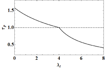
Figure 1: Passage time $\tau_{p}$ versus measurement precision parameter, $\lambda_{t}$. A unit system in which $\hbar=V_{0}$=1 is used. The passage time at the exceptional point is indicated by the dotted lines.

4 Dynamics of quantum correlations and entanglement of observed qubits

We consider a composite system consisting of the two-level system ($s$), the source of the external potential $V(t)$ (denoted by $r$), and the external monitoring device (denoted by $d$), with a measurement precision, $E_{r}$. During the measurement procedure, the composite state $\left|\psi_{i}\right\rangle=\left|1\right\rangle_{s}\left|0\right\rangle_{r}\left|0\right\rangle_{d}$ evolves under the action of the Hamiltonians of Eq. (3) and (5) as

$$\left|\psi_{t}\right\rangle=\xi_{t}\left|1\right\rangle_{s}\left|0\right\rangle_{r}\left|0\right\rangle_{d}+\eta_{t}\left|0\right\rangle_{s}\left|1\right\rangle_{r}\left|0\right\rangle_{d}+\chi_{t}\left|0\right\rangle_{s}\left|0\right\rangle_{r}\left|1\right\rangle_{d}$$ (19)

where $|\xi_{t}|^{2}=P_{11}$, $|\eta_{t}|^{2}=P_{10}$ (see Eqs.  (9) to (12) ) and $|\chi_{t}|^{2}=1-|\xi_{t}|^{2}-|\eta_{t}|^{2}$. We note that in the composite state $\left|\psi_{i}\right\rangle=\left|1\right\rangle_{s}\left|0\right\rangle_{r}\left|0\right\rangle_{d}$, only a single excitation is initially present in the qubit, and accordingly only one of the considered subsystem ($s$, $r$ or $d$) is present in the $\left|1\right\rangle$ state. Thus in the absence of excitations in either the system $s$ or source of external potential $r$, it is considered that the detector states are excited.

In this Section, we focus on the detailed analysis of a system of two noninteracting subsystems ($s_{1},s_{2}$) where each subsystem is equivalent to the two-level system $s_{1}$ in Eq.  (19). Each subsystem is monitored by its respective observers ($d_{1},d_{2}$), with identical characteristics such that the measurement precision, $E_{r}$ is the same for both detectors. The Hamiltonian of the total system is thus given by the sum of the Hamiltonians of the two noninteracting subsystems, $\hat{H}_{T}=\hat{H}_{1}+\hat{H}_{2}$, where $H_{i}$ (i=$1,2$) have the form given in Eq.  (5). In order to examine the response of two initially entangled qubits which are monitored by $d_{1},d_{2}$, we assume that the pair of qubits are in an initial state of the form

$$\left|\Psi_{i}\right\rangle=\left(a\left|0_{s_{1}}0_{s_{2}}\right\rangle+b\left|1_{s_{1}}1_{s_{2}}\right\rangle\right)\left|0_{r_{1}}0_{r_{2}}\right\rangle\left|{0}_{d_{1}}{0}_{d_{2}}\right\rangle,$$ (20)

where $a,b$ are complex parameters, and the source of external potential $r$ and detector $d$ are present in their vacuum state. Using Eq.  (19), the composite system, $\left|\Psi_{i}\right\rangle$ evolves as

$$\left|\Psi_{t}\right\rangle=a\left|0_{s_{1}}0_{s_{2}}\right\rangle\left|0_{r_{1}}0_{r_{2}}\right\rangle\left|0_{d_{1}}0_{d_{2}}\right\rangle+b\left|\psi_{t}\right\rangle_{1}\left|\psi_{t}\right\rangle_{2},$$ (21)

By tracing out the degrees of freedom of the qubits associated with the sources of external potential $r_{1},r_{2}$, and detectors $d_{1},d_{2}$, the reduced density matrix of the bipartite two-qubit system at time $t$ is obtained in the basis $\{\left|00\right\rangle,\left|01\right\rangle,\left|10\right\rangle,\left|11\right\rangle\}$ as

$${\rho}_{s_{1}s_{2}}(t)=\left(\begin{array}[]{cccc}|a|^{2}+|b|^{2}(1-|\xi_{t}|^{2})^{2}&0&0&ab^{\ast}(\xi_{t}^{\ast})^{2}\\ 0&|b|^{2}|\xi_{t}|^{2}(1-|\xi_{t}|^{2})&0&0\\ 0&0&|b|^{2}|\xi_{t}|^{2}(1-|\xi_{t}|^{2})&0\\ a^{\ast}b\xi_{t}^{2}&0&0&|b|^{2}|\xi_{t}|^{4}\\ \end{array}\right)\\$$ (22)

where we have assumed identical characteristics for the two detectors. A similar analysis involving the evolution of a multipartite state influenced by the coefficients $a,b$ have been performed for the excitonic qubit system, but not in the current context of quantum measurements, in earlier works [47, 48].

The concurrence of the density matrix in Eq. (22) is obtained as [49]

$$\mathcal{C}_{s}(t)=\mathrm{max}\left\{0,2|b||\xi_{t}|^{2}[|a|-|b|(1-|\xi_{t}|^{2})]\right\}.$$ (23)

The concurrences, $\mathcal{C}_{r}(t)$ and $\mathcal{C}_{d}(t)$ associated respectively with the two-potential source and two-detector density matrices at time $t$ are obtained by respective substitutions $\xi_{t}\rightarrow\eta_{t}$ and $\xi_{t}\rightarrow\chi_{t}$ in Eq. (23).

4.1 Dynamics of quantum correlations near exceptional points

While the entanglement measure such as concurrence has useful features, a different correlation measure known as the quantum discord is more robust as it captures a nonlocal correlations not present in the entanglement measure. The quantum discord is non vanishing in states which has zero entanglement, however its evaluation involves lengthy optimization procedures and analytical expressions are known exist only in a few limiting cases. It would be interesting to investigate the change in the quantum correlation ($Q$) [50, 51] which has similar features as the quantum discord introduced by Olliver and Zurek [52] in the context of the two-qubit system undergoing quantum measurements. In particular, the dynamics of non-classical correlations, especially near the exceptional point remains unexplored in earlier works.

The quantum correlation $Q$ is obtained by computing the classical correlation $C$ in the first instance. For the two-qubit case, $C$ is obtained [50, 51] using $C(\rho_{s_{1}s_{2}})\equiv\max_{\{\Pi_{j}\}}[S(\rho_{s_{1}})-S_{\{\Pi_{j}\}}(\rho_{s_{1}|s_{2}})]$, where the maximum is determined from the set of positive-operator-valued measurements $\{\Pi_{j}\}$ in the adjacent partition $s_{2}$. $Q$ is evaluated using the quantum mutual information $I$, which is given by the sum of classical correlation and quantum correlations. It is to be noted that the quantum correlations is dependent on the position of the partition on which measurements are carried out, i.e., $Q$ is asymmetric. $Q$ becomes symmetric only for $S(\rho_{1})=S(\rho_{2})$ where $S(\rho)$ denotes the Von Neumann entropy of state $\rho$).

Following the analytical approach in Ref.[53, 54, 55], expressions for the $C$ and $Q$ associated with the qubit-qubit bipartite system, are obtained as

$$C_{s}(t) = Q_{s}(t)={H}(|b\xi_{t}|^{2})$$ (24)

$$- {H}\left(\frac{1}{2}\left[1+\sqrt{1-4|b\xi_{t}(1-\xi_{t}^{2})^{1/2}|^{2}}\right]\right),$$

where the Shannon entropy ${H}(x)=-x{{log}}_{2}x-(1-x){{log}}_{2}(1-x)$. Analogous expressions for $C_{r},Q_{r}$ and $C_{d},Q_{d}$ associated respectively with the two-potential source and two-detector density matrices at time $t$ are obtained by respective substitutions $\xi_{t}\rightarrow\eta_{t}$ and $\xi_{t}\rightarrow\chi_{t}$ in Eq. (24). It is to be noted that for all bipartite systems ($s_{1}-s_{2}$, $r_{1}-r_{2}$ and $d_{1}-d_{2}$) the classical correlations are equal to quantum correlations, so that the quantum mutual information is twice that evaluated for $Q$ for the bipartite systems.

In Fig. 2a to 2f, the quantum correlations (as a function of time $t$ and measurement precision term $\lambda_{t}$) associated with the qubit-qubit, potential-potential sources and detector-detector bipartite systems are illustrated alongside their corresponding concurrence measures. For convenience, we have used a unit system in which $\hbar=V_{0}$=1, so that time $t$ and the measurement precision parameter $\lambda_{t}$ are unitless as well. The figure shows the progressive transfer of initial correlations and concurrence between qubits to the potential-potential source qubits and then to creation of quantum correlations and entanglement between the two detector systems with increasing $\lambda_{t}$. The quantum correlations remains more robust during this transfer. As $\lambda_{t}$ increases, the system moves closer to the exceptional point and the quantum correlations between the monitored (monitoring) systems is considerably decreased (increased). As shown in Fig. 3, the quantum correlations in the detector-detector bipartite system reaches near unity values for a range of the parameter $b$ at the exceptional point and at the end of the measurement duration. It is apparent that the loss of information associated with the formation of exceptional points in the qubit-qubit bipartite system correlates to increased quantum correlations in the detector-detector bipartite system. The results in Fig. 2 support the view that the collapse of the observed state vector implies the transfer of the wave function s amplitude, and indirectly quantum information away from the interaction space. In this regard the non-Hermitian description of quantum measurement is consistent with increased information transfer to the detector system in the case of highly precise measurements.

The results thus far have been obtained for a case where the two qubits are in a pure entangled state at $t=$0 as given in Eq.  (20). A different initial state may yield some changes in the magnitude of the concurrence and quantum correlations obtained here, however the overall trend in changes of these measures with $t$ and $\lambda_{t}$ is expected to be the same as illustrated in Fig. 2. In summary, the results indicate that a highly precise observer can diminish the non-classical correlation shared between two subsystems undergoing measurements, with the tendency to do so increasing with measurement precision.

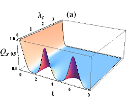
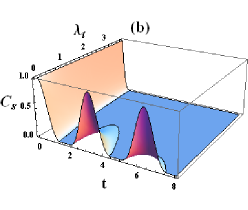
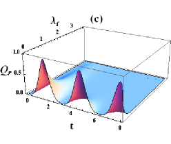
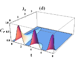
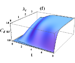
Figure 2: (a) Two-qubit quantum correlation $Q_{s}$ and (b) Two-qubit concurrence $\mathcal{C}_{s}$ as function of time $t$ and measurement precision parameter $\lambda_{t}$ with initial amplitude parameter $b$=0.75. A unit system in which $\hbar=V_{0}=\Delta E$=1, $\tau$=8 is used, hence 0$\leq t\leq$ 8 and $\lambda_{t}=\frac{1}{(4E_{r})^{2}}$
(c) Two-potential source quantum correlation $Q_{r}$ and (d) Concurrence $\mathcal{C}_{r}$ as function of time $t$ and measurement precision parameter $\lambda_{t}$ with the initial amplitude parameter $b$=0.75 .
(e) Two-detector quantum correlation $Q_{d}$ and (f) Two-detector concurrence $\mathcal{C}_{d}$ as function of time $t$ and measurement precision parameter $\lambda_{t}$ with initial amplitude parameter $b$=0.75 .

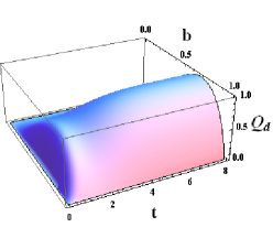
Figure 3: Two-detector quantum correlation $Q_{d}$ as function of time $t$ and initial amplitude parameter $b$ at the exceptional point where $\lambda_{t}$=4.

4.2 Relationship between the exceptional point and appearance of non-classical correlations

The exact relationship between the occurrence of the exceptional points and the quantum correlations between the various parties (qubit, detectors) involved is not immediately clear, however the transfer of non-classical quantum correlations from one subsystem to another appear to underpin quantum measurements. The results obtained in this work, show that as the system moves closer to the exceptional point (small error/duration), the quantum correlation between the monitored (monitoring) systems is considerably decreased (increased). Moreover the passage time from one state to another at the exceptional point is correlated with enhanced quantum correlation or non-classical correlations between the measuring instruments. This is possibly consistent with the fact that loss of quantum information due to the merging of eigenfunctions at the exceptional point is translated to greater involvement of the unobserved states of the measuring devices. The exact mathematical formulations underlying these non-trivial correlations and exchanges may require greater understanding of the topological fabric space in which the exceptional points are embedded, and such non-trivial spaces may facilitate examination of the degeneracies that is unique to exceptional points. For instance, Nesterov et. al. [4, 23] has modelled the quantum evolution dynamics of the complex sphere on a one-sheeted two-dimensional hyperboloid space in terms of two inner parameters and obtained results (such as distances between the final and initial states), highlighting the importance of the geometric features of the dynamics of non-Hermitian systems. Accordingly, greater insight on the underlying mechanism by which entities such as entanglement and non-classical correlations of quantum systems are transferred from one subsystem to another may be revealed via use of the geometric approach developed by Anandan and Aharonov [22].

5 Conclusion

In this work, we have examined the appearance of exceptional points and passage times in a two-level system which admits an effective non-Hermitian description via the Feynman’s path integral formalism and based on the restricted path integral approach. The two dimensional model using an oscillatory (in time) potential as off-diagonal perturbation is solved analytically and the time dependent transition probabilities are evaluated. Their explicit dependence on the measurement duration time and error demonstrate that at resonance frequency, there are two regimes depending on error and measurement duration: incoherent tunnelling (small error/duration) and coherent tunnelling (large error/duration); these two regimes merge at the exceptional point at which point the passage time is noted to be half of the measurement duration. The entanglement dynamics of a multipartite system consisting of the correlated qubits, the sources of external potential and monitoring devices is examined using correlation measures such as concurrence and quantum correlations. The results indicate that the quantum correlations between the monitored (monitoring) systems is considerably decreased (increased) as the measurement precision nears the exceptional point. Quantum correlations shows greater robustness than the concurrence measure during the measurement process, which is expected due to the richness of quantum correlations intrinsically present in the former entity.

Overall the results in this study show that quantum measurement procedures with a select range of precision, can be used to transfer quantum correlations present as non-classical quantum correlations in one system to remote systems with a certain degree of reliability. To this end, future investigations involving measures such as the fidelity may be used to analyse the reliability range of information transfer. The results presented here may also be extended to examine high efficiencies of energy transfer in photosynthetic systems [20, 56] and quantum system relevant to quantum computation [57]. However the explicit link between the passage time and appearance of non-classical correlations needs further study, possibly requiring geometric approaches as proposed in Ref. [22]. Nevertheless, the appearance of singularities such as the exceptional points in highly precise measurements, as predicted in this work, may provide useful guidelines to their detection in experimental studies involving quantum measurement in optics and nanostructure systems [28, 32, 58, 59]. Accordingly the results obtained here may facilitate the testing ground of pseudo-Hermitian quantum mechanics using appropriate quantum measurement procedures in nanostructured devices.

6 Acknowledgments

The author gratefully acknowledges useful comments from the anonymous referees. This research was undertaken on the NCI National Facility in Canberra, Australia, which is supported by the Australian Commonwealth Government.

7 References

References

- [1] C. M. Bender, Reports on Progress in Physics 70, 947 (2007).
- [2] C. M. Bender and S. Boettcher, Phys. Rev. Lett . 80, 5243 (1998).
- [3] I. Rotter, J. Phys. A: Math. Theor. 42, 153001 (2009).
- [4] A. I. Nesterov, Physics Letters A 373, 3629 (2009).
- [5] C. M. Bender, Rep. Prog. Phys. 70, 947 (2007).
- [6] P. E. Assis and A. Fring, J. Phys. A: Math. Theor. 41, 244002 (2008).
- [7] A. Mostafazadeh, Phys. Rev. Lett. 99 130502 (2007).
- [8] A. Mostafazadeh, Int. J. Geom. Meth. Mod. Phys. 7, 1191 (2010).
- [9] C. M. Bender, D. C. Brody, H. F. Jones, and B. K. Meister, Phys. Rev. Lett. 98, 040403 (2007).
- [10] W. D. Heiss, Eur. Phys. J. D 29, 429 (2004); Czech. J. Phys. 54, 1091 (2004).
- [11] E.Hernandez, A. Jauregui and A. Mondragon Phys. Rev. E 84, 046209 (2011).
- [12] Z. H. Musslimani, K. G. Makris, R. El-Ganainy, and D. N. Christodoulides, Phys.Rev.Lett. 100, 030402 (2008).
- [13] L. Jin and Z. Song, Phys. Rev. A 84, 042116 (2011).
- [14] O. Atabeck and R. Lefebvre, J. Phys. Chem. A 114, 3031 (2010).
- [15] M. V. Berry and M. R. Dennis, Proc. R. Soc. London A 459, 1261 (2003).
- [16] B. Dietz, H. L. Harney, O. N. Kirillov, M. Miski-Oglu, A. Richter, and F. Schäfer, Phys. Rev. Lett. 106, 150403 (2011).
- [17] M. Philipp, P. von Brentano, G. Pascovici, and A. Richter, Phys. Rev. E 62, 1922 (2000).
- [18] A. Goetschy and S. E. Skipetrov Phys. Rev. E 84, 011150 (2011).
- [19] S.-B. Lee, J. Yang, S. Moon, S.-Y. Lee, J.-B. Shim, S. W. Kim, J.-H. Lee, and K. An, Phys. Rev. Lett. 103, 134101 (2009).
- [20] A. Thilagam, J. Chem. Phys. 136, 065104 (2012).
- [21] W. D. Heiss, Phys. Rev. E 61, 929 (2000).
- [22] J. Anandan and Y. Aharonov, Phys. Rev. Lett. 65, 1697 (1990).
- [23] A.I. Nesterov, SIGMA 5 069 (2009).
- [24] J. von Neumann, “Mathematical Foundations of Quantum Mechanics,” Princeton University Press, Princeton, (1955).
- [25] H. D. Zeh, Found. Phys. 1, 69 (1970).
- [26] A. G. Kofman, G. Kurizki, Nature 405, 546 (2000); Phys. Rev.A 54, 3750(R)(1996).
- [27] B. Misra and E. C. G. Sudarchan, J. Math. Phys. 18, 758 (1977).
- [28] P. Busch, P. J. Lahti, and P. Mittelstaedt, “The Quantum Theory of Measurement,” Springer-Verlag, Berlin, (1991).
- [29] H. M. Wiseman, Quantum Semiclass. Opt. 8 205 (1996)
- [30] W.M. Itano, D. J. Heinzen, J. J. Bollinger and D. J. Wineland, Phys. Rev.A 41, 2295 (1990).
- [31] P. Facchi and S. Pascazio, J. Phys. A: Math. Theor. 41 493001 (2008); P. Facchi and S. Pascazio, Phys. Rev. Lett. 89, 080401 (2002).
- [32] V. B. Braginsky and F. Ya. Khalili, “Quantum Measurement”, K. S. Thorne editor (Cambridge University Press, Cambridge) (1992), and references cited therein.
- [33] M. B. Mensky, “Continuous Quantum Measurements and Path-Integrals” (Institute of Physics Publishers, Bristol and Philadelphia) (1993).
- [34] W. H. Zurek, Phys. Today 44 (10), 36 (1991).
- [35] M. Schlosshauer, “Decoherence and the Quantum-to-Classical Transition”, Springer-Verlag, (2008).
- [36] J. Kofler and C. Brukner, Phys. Rev. Lett. 101, 090403 (2008).
- [37] J. C. Garrison and E. M. Wright, Phys. Lett. A, 128 177 (1988).
- [38] R. P. Feynman and A. R. Hibbs, “Quantum Mechanics and Path Integrals”, (McGraw-Hill, New York) (1965).
- [39] R. P. Feynman, Rev. Mod. Phys. 20, 367 (1948).
- [40] M. B. Mensky, Phys. Rev. D 20, 384 (1979); Sov. Phys. JETP 50, 667 (1979).
- [41] M. B. Mensky, R. Onofrio, and C. Presilla, Phys. Rev. Lett. 70, 2825 (1993).
- [42] M. B. Mensky, R. Onofrio, and C. Presilla, Phys. Lett. A 161, 236 (1991).
- [43] R. Onofrio, C. Presilla, and U. Tambini, Phys. Lett. A 183, 135 (1993).
- [44] C. A. Stafford and B. R. Barrett, Phys. Rev. C 60, 051305 (1999).
- [45] D. C. Brody, J. Phys. A: Math. Gen. 36 5587 (2003).
- [46] D. C. Brody and D. W. Hook, J. Phys. A: Math. Gen. 39 L167 (2006).
- [47] A. Thilagam, J. Phys. A: Math. Theor. 43, 155301 (2010).
- [48] A. Thilagam , J. Phys. A: Math. Theor. 42, 335301 (2009).
- [49] V. Coffman, J. Kundu and W. K. Wootters, Phys. Rev. A 61, 052306 (2000).
- [50] L. Henderson and V. Vedral, J. Phys. A 34, 6899 (2001).
- [51] V. Vedral, Phys. Rev. Lett. 90, 050401 (2003).
- [52] H. Ollivier and W. H. Zurek, Phys. Rev. Lett. 88, 017901 (2001).
- [53] M. Ali, A. R. P. Rau, and G. Alber, Phys. Rev. A 81, 042105 (2010).
- [54] M. Ali, A. R. P. Rau, and G. Alber, Phys. Rev. A 82, 069902(E) (2010).
- [55] C.Z. Wang, C.X. Li, L.Y. Nie and J.F. Li, J. Phys. B: At. Mol. Opt. Phys. 44, 015503 (2011).
- [56] A. Thilagam, J. Chem. Phys. 136, 175104 (2012).
- [57] M. A. Nielsen and I.L. Chuang, Quantum Computation and Quantum Information (Cambridge University Press, Cambridge, U.K., 2000).
- [58] M. A. Hall, J. B. Altepeter and P. Kumar Optics Express 17, 14558(2009).
- [59] W. Tittel, J. Brendel, H. Zbinden, and N. Gisin, Phys. Rev. Lett. 81, 3563 (1998).